All order $\bm{\alpha^{\prime}}$-expansion of superstring trees from the Drinfeld associator

Abstract

We derive a recursive formula for the $\alpha^{\prime}$-expansion of superstring tree amplitudes involving any number $N$ of massless open string states. String corrections to Yang-Mills field theory are shown to enter through the Drinfeld associator, a generating series for multiple zeta values. Our results apply to any number of spacetime dimensions or supersymmetries and chosen helicity configurations.

I Introduction

Scattering amplitudes are the most fundamental observables in both quantum field theory and string theory. In recent years, numerous hidden structures underlying the S-matrix have been revealed in both disciplines. Several of these discoveries can be attributed to and have benefited from the close interplay between amplitudes of string theory in the low-energy limit and supersymmetric Yang-Mills (YM) field theory.

A main challenge in the study of field theory amplitudes originates from the transcendental functions in their quantum corrections. Novel mathematical techniques such as the symbol GoncharovOrig helped to streamline the polylogarithms and multiple zeta values (MZVs) in loop amplitudes of (super-)YM theory. In string theory, MZVs appear in the $\alpha^{\prime}$-corrections already at tree level due to the exchange of infinitely many heavy vibrational modes. These effects are encoded in integrals over world-sheets of genus zero.

The study of $\alpha^{\prime}$-expansions in the superstring tree-level amplitude is interesting from both a mathematical and a physical point of view. On the one hand, the pattern of MZVs appearing therein can be understood from an underlying Hopf algebra structure Schlotterer:2012ny . On the other hand, explicit knowledge of the associated string corrections is crucial for the classification of candidate counterterms in field theories with unsettled questions about their UV properties Beisert:2010jx .

In spite of technical advances to evaluate $\alpha^{\prime}$-expansions for any multiplicity polylog , compact and straightforwardly applicable formulae for string corrections are still lacking. This letter closes this gap by describing a novel method to recursively determine the $\alpha^{\prime}$-dependence of $N$-point trees through the generating function of MZVs – the Drinfeld associator. Its connection with superstring amplitudes – in particular the common pattern of MZV appearance – was firstly pointed out in Drummond:2013vz . Our techniques are based on the Knizhnik-Zamolodchikov (KZ) equation Knizhnik:1984nr obeyed by world-sheet integrals and thereby resemble ideas in field theory to determine loop integrals Henn:2013pwa . Along the lines of Terasoma , the associator is shown to connect boundary values, given by $N$-point and $(N-1)$-point disk amplitudes, respectively. The method presented in this article bypasses the cumbersome direct evaluation of world-sheet integrals and reduces their $\alpha^{\prime}$-expansions to simple matrix multiplications. Apart from its conceptual accessibility, it substantially reduces the computational effort in deriving the explicit form of $\alpha^{\prime}$-corrections.

A. The structure of disk amplitudes: The color-ordered $N$-point disk amplitude $A_{\textrm{open}}(\alpha^{\prime}):=A_{\textrm{open}}(1,2,\ldots,N;\alpha^{\prime})$ was computed in Mafra:2011nv ; Mafra:2011nw based on pure spinor cohomology methods Mafra:2010jq . Its entire polarization dependence was found to enter through color-ordered tree amplitudes $A_{\textrm{YM}}$ of the underlying YM field theory which emerges in the point particle limit $\alpha^{\prime}\rightarrow 0$:

$$A_{\textrm{open}}(\alpha^{\prime})=\sum_{\sigma\in S_{N-3}}F^{\sigma}(\alpha^{\prime})\,A_{\textrm{YM}}^{\sigma}\,.$$ (1)

The $(N-3)!$ linearly independent BCJ subamplitudes $A_{\textrm{YM}}(1,\sigma(2,3,\ldots,N-2),N-1,N)$ are grouped into a vector $A_{\textrm{YM}}^{\sigma}$. The objects $F^{\sigma}(\alpha^{\prime})$ describe string corrections to YM amplitudes and will be recursively determined as the main result of this letter. They are generalized Selberg integrals Selberg over the boundary of the open string world-sheet of disk topology:

$$F^{\sigma} =(-1)^{N-3}\prod_{i=2}^{N-2}\int_{z_{i}<z_{i+1}}\!\!\!\!\!\mathrm{d}z_{i}\ {\cal I}\,\sigma\bigg{\{}\prod_{k=2}^{N-2}\sum_{j=1}^{k-1}\frac{s_{jk}}{z_{jk}}\bigg{\}}\,,$$ (2)

$${\cal I} =\prod_{i<j}^{N-1}|z_{ij}|^{s_{ij}}\ ,\ \ \ (z_{1},z_{N-1},z_{N})=(0,1,\infty)\,.$$ (3)

The $S_{N-3}$ permutation $\sigma$ acts on labels $2,3,\ldots,N\!-\!2$ of $z_{ij}:=z_{i}\!-\!z_{j}$ and of the dimensionless Mandelstam invariants

$$s_{i_{1}i_{2}\ldots i_{p}}=\alpha^{\prime}(k_{i_{1}}+k_{i_{2}}+\ldots+k_{i_{p}})^{2}\ ,$$ (4)

which carry the $\alpha^{\prime}$-dependence of the string amplitude (1). The $k_{i}$ denote external on-shell momenta. Hence, the $s_{ij}$-expansion of the integrals (2) encodes the low energy behaviour of superstring tree amplitudes.

B. Multiple zeta values: As discussed in both mathematics Aomoto ; Terasoma ; Francis and physics Stieberger:2009rr ; Mafra:2011nw ; Schlotterer:2012ny literature, the $\alpha^{\prime}$-expansion of Selberg integrals involves (products of) MZVs. They can be defined by iterated integrals over differential forms $\omega_{0}:=\frac{\mathrm{d}z}{z}$ and $\omega_{1}:=\frac{\mathrm{d}z}{1-z}$

$$\zeta_{n_{1},\ldots,n_{r}}=\!\!\!\!\!\!\!\!\!\!\!\!\int\limits_{0<z_{i}<z_{i+1}<1}\!\!\!\!\!\!\!\!\!\!\!\!\omega_{1}\underbrace{\omega_{0}\ldots\omega_{0}}_{n_{1}-1}\omega_{1}\underbrace{\omega_{0}\ldots\omega_{0}}_{n_{2}-1}\ldots\omega_{1}\underbrace{\omega_{0}\ldots\omega_{0}}_{n_{r}-1}$$ (5)

where $n_{j}\in\mathbb{N}$ and $n_{r}\geq 2$. The overall weights $\sum_{j=1}^{r}n_{j}$ of MZV factors match the power of $\alpha^{\prime}$ in the string amplitudes’ expansion. Instead of labeling MZVs by the set of $n_{j}$, one can equivalently encode the integrand of eq. (5) in a word $w$ in the alphabet $\{0,1\}$ (i.e. $w\in\{0,1\}^{\times}$) where the function $w[\omega_{0},\omega_{1}]$ translates this word into sequences of $\{\omega_{0},\omega_{1}\}$ Drummond:2013vz :

$$\zeta_{(w)}:=\!\!\!\!\!\!\!\!\!\!\!\!\int\limits_{0<z_{i}<z_{i+1}<1}\!\!\!\!\!\!\!\!\!\!\!\!w[\omega_{0},\omega_{1}]\,.$$ (6)

The pattern of MZVs in the $\alpha^{\prime}$-expansion of (2) has been revealed in Schlotterer:2012ny on the basis of a Hopf algebra structure.

C. The Drinfeld associator: Consider the KZ equation with $z_{0}\in\mathbb{C}\backslash\{0,1\}$ and Lie-algebra generators $e_{0},e_{1}$:

$$\frac{\mathrm{d}{\bf{\hat{F}}}(z_{0})}{\mathrm{d}z_{0}}=\left(\frac{e_{0}}{z_{0}}+\frac{e_{1}}{1-z_{0}}\right){\bf{\hat{F}}}(z_{0})\ .$$ (7)

The solution ${\bf{\hat{F}}}(z_{0})$ of the KZ equation takes values in the vector space the representation of $e_{0}$ and $e_{1}$ is acting upon. The regularized boundary values

$$C_{0}:=\lim_{z_{0}\rightarrow 0}z_{0}^{-e_{0}}{\bf{\hat{F}}}(z_{0})\ ,\ \ \ C_{1}:=\lim_{z_{0}\rightarrow 1}(1-z_{0})^{e_{1}}{\bf{\hat{F}}}(z_{0})\,$$ (8)

are related by the Drinfeld associator Drinfeld:1989st ; Drinfeld2

$$C_{1}=\Phi(e_{0},e_{1})\,C_{0}\ ,$$ (9)

where $C_{0}$, $C_{1}$ and $\Phi$ take values in the universal enveloping algebra of the Lie algebra generated by $e_{0}$ and $e_{1}$. The regularizing factors $z_{0}^{-e_{0}}$ and $(1-z_{0})^{e_{1}}$ are included into eq. (8) as to render the $z_{0}\rightarrow 0,1$ regime of ${\bf{\hat{F}}}(z_{0})$ real-single-valued. In the notation of eq. (6), the Drinfeld associator can be represented as a generating series of MZVs Le :

$$\Phi(e_{0},e_{1})=\sum_{w\in\{0,1\}^{\times}}\tilde{w}[e_{0},e_{1}]\zeta_{(w)}\,,$$ (10)

where $\tilde{w}$ denotes the reversal of the word $w$. The series expansion of eq. (10) in a basis of MZVs starts with the following commutators $[\cdot,\cdot]$:

$$\Phi(e_{0},e_{1}) =1+\zeta_{2}[e_{0},e_{1}]+\zeta_{3}[e_{0}-e_{1},[e_{0},e_{1}]]$$

$$+\zeta_{4}([e_{0},[e_{0},[e_{0},e_{1}]]]+\tfrac{1}{4}[e_{1},[e_{0},[e_{1},e_{0}]]]$$

$$\ \ -[e_{1},[e_{1},[e_{1},e_{0}]]]+\tfrac{5}{4}[e_{0},e_{1}]^{2})+\ldots\;\;\ ,$$ (11)

D. Main result: In this letter, we identify the Drinfeld associator $\Phi$ as the link between $N$-point string amplitudes and those of multiplicity $N-1$. Thus, starting from the $\alpha^{\prime}$-independent three-point level, one can build up any tree-level string amplitude recursively.

We will construct a matrix representation for the associator arguments $e_{0}$ and $e_{1}$ in section I.C for each multiplicity. Starting with a boundary value $C_{0}$ containing the world-sheet integrals for the $(N\!-\!1)$-point amplitude, eq. (9) yields a vector $C_{1}$, which we will show to encode the integrals eq. (2) for multiplicity $N$. Consequently, one can express the $N$-point world-sheet integrals $F^{\sigma}$ in terms of those at $(N\!-\!1)$-points

$$F^{\sigma_{i}} =\!\sum_{j=1}^{(N-3)!}\!\big{[}\Phi(e_{0},e_{1})\big{]}_{ij}\ F^{\sigma_{j}}\big{|}_{k_{N-1}=0},$$ (12)

where the soft limit $k_{N-1}=0$ gives rise to $(N-1)$-point integrals on the right hand side

$$F^{\sigma(23\ldots N-2)}\big{|}_{k_{N-1}=0} =\left\{\begin{array}[]{cl}\!F^{\sigma(23\ldots N-3)}\!&\textrm{if}\,\,\sigma(N\!-\!2)\!=\!N\!-\!2\\ 0\!\!&\textrm{otherwise\,.}\end{array}\right.$$ (15)

The permutations $\sigma_{i}$ are canonically ordered in eq. (12).

II The method

The backbone of the recursion eq. (12) is a vector $\bf{\hat{F}}$ of auxiliary functions and a corresponding matrix representation of $e_{0},e_{1}$ such that the KZ equation (7) holds . Moreover, the boundary values $C_{0}$ and $C_{1}$ derived from $\bf{\hat{F}}$ via eq. (8) need to reproduce basis functions eq. (2) of multiplicity $N-1$ and $N$, respectively. As we will see, these requirements are met by components

$$\hat{F}_{\nu}^{\sigma} (z_{0},s_{0k})=(-1)^{N-3}\int^{z_{0}}_{0}\mathrm{d}z_{N-2}\prod_{i=2}^{N-3}\int_{0}^{z_{i+1}}\mathrm{d}z_{i}\ {\cal I}$$

$$\times\prod_{k=2}^{N-2}z_{0k}^{s_{0k}}\sigma\bigg{\{}\prod_{k=2}^{\nu}\sum_{j=1}^{k-1}\frac{s_{jk}}{z_{jk}}\prod_{m=\nu+1}^{N-2}\sum_{n=m+1}^{N-1}\frac{s_{mn}}{z_{mn}}\bigg{\}}\,.$$ (16)

The vector $\bf{\hat{F}}$ is composed from $N\!-\!2$ subvectors $\hat{F}_{\nu}$ of length $(N\!-\!3)!$. Numbered by $\nu\!=\!1,2,..,N\!-\!2$, they appear in decreasing order, that is, ${\bf{\hat{F}}}=(\hat{F}_{N-2},\hat{F}_{N-3},\ldots,\hat{F}_{1})$. Entries of the $\hat{F}_{\nu}$ are labeled by permutations $\sigma\in S_{N-3}$.

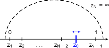
Figure 1: Worldsheet with an auxiliary position $z_{0}$.

The integrals in eq. (16) generalize the functions eq. (2) through an auxiliary world-sheet position $z_{0}$ and auxiliary Mandelstam variables $s_{0k}$. This $z_{0}$ enters in the integration limit of the outermost integral as well as in the deformation $\prod_{k=2}^{N-2}(z_{0k})^{s_{0k}}$ of the Koba-Nielsen factor ${\cal I}$ and serves as the differentiation variable for the KZ equation (7). As visualized in the above figure, the position $z_{0}$ downscales the integration domain on the disk boundary and thus interpolates between world-sheet-configurations of an $N$-point and $(N\!-\!1)$-point tree amplitude.

At $z_{0}\!=\!1$ and $s_{0k}\!=\!0$ – in absence of the augmentation – the functions $\hat{F}_{\nu}^{\sigma}$ in eq. (16) approach the integrals $F^{\sigma}$ in the amplitude for any $\nu$. In this regime, $\nu$ labels different equivalent representations polylog of the integrals eq. (2).

Matching the length of the auxiliary vector, $e_{0}$ and $e_{1}$ in eq. (7) are $(N\!-\!2)!\times(N\!-\!2)!$-matrices. It is known Terasoma that their entries are linear forms on $s_{ij}$. They can be determined by matching the $z_{0}$ derivatives of $\hat{F}^{\sigma}_{\nu}$ with the right hand side of the KZ equation (7). Once the resulting matrices $e_{0}$ and $e_{1}$ are available, one can calculate the Drinfeld associator to any desired order employing its series expansion eq. (10). Having set up the KZ equation (7) for the auxiliary function $\bf{\hat{F}}$, we will now relate its regularized boundary terms eq. (8) to the integrals eq. (2) in the string amplitude.

A. The $\bm{z_{0}\rightarrow 0}$ boundary value $\bm{C_{0}}$: The boundary term $C_{0}$ is determined by taking the limit $z_{0}\!\rightarrow\!0$ of $z_{0}^{-e_{0}}{\bf{\hat{F}}}(z_{0})$. This amounts to squeezing the world-sheet positions $z_{2},\ldots,z_{N-2}$ into an interval $[0,z_{0}]$ of vanishing size, see the above figure. This effectively removes one of the $N-3$ integrations and makes contact with the $(N-1)$-point problem. Let us make this more precise: The first $(N\!-\!3)!$ components of ${\bf{\hat{F}}}(z_{0}\!\rightarrow\!0)$ at $\nu=N\!-\!2$,

$$\hat{F}_{N-2}^{\sigma}(z_{0}\rightarrow 0,s_{0i})=z_{0}^{s_{\textrm{max}}}F^{\sigma}\big{|}_{s_{i,N-1}=s_{0i}}+{\cal O}(s_{0i})\,,$$ (17)

involve the eigenvalue $s_{\textrm{max}}\!=\!s_{12\ldots N-2}\!+\!\sum_{j=2}^{N-2}s_{0j}$ of $e_{0}$ Terasoma . The remaining subvectors of ${\bf{\hat{F}}}(z_{0}\!\rightarrow\!0)$ at $\nu\leq N\!-\!3$ are suppressed by $N-2-\nu$ powers of $z_{0}$ and do not contribute to $C_{0}$. The action of $z_{0}^{-e_{0}}$ compensates the $z_{0}$ dependence of the resulting vector $(z_{0}^{s_{\textrm{max}}}F^{\sigma},{\bf 0}_{(N-3)(N-3)!})$.

The desired $(N-1)$-point integrals can be achieved through a soft limit $k_{N-1}\rightarrow 0$, see (15). This can be realized by setting $s_{0i}=s_{i,N-1}=0$ in eq. (17) which converts the subvector $\hat{F}^{\sigma}_{N-2}$ into $(N-1)$-point data

$$C_{0}=(F^{\sigma}\big{|}_{k_{N-1}=0},{\bf 0}_{(N-3)(N-3)!})\ .$$ (18)

B. The $\bm{z_{0}\rightarrow 1}$ boundary value $\bm{C_{1}}$: The $z_{0}\rightarrow 1$ regime of $(1-z_{0})^{e_{1}}{\bf{\hat{F}}}(z_{0})$ underlying $C_{1}$ restores the integration domain of the $N$-point functions eq. (2). Considering the schematic form of the first $(N\!-\!3)!$ rows in

$$(1-z_{0})^{e_{1}}=\left(\begin{array}[]{cc}\bm{1}_{(N\!-\!3)!\times(N\!-\!3)!}&{\bf 0}_{(N\!-\!3)!\times(N\!-\!3)(N\!-\!3)!}\\ \vdots&\vdots\end{array}\right)$$ (19)

we can neglect all components of ${\bf{\hat{F}}}(z_{0}\rightarrow 1)$ except

$$\hat{F}_{N-2}^{\sigma}(z_{0}\rightarrow 1,s_{0i})=F^{\sigma}+{\cal O}(s_{0i})\ .$$ (20)

Setting $s_{0i}=0$ as motivated in section II.A leads to

$$C_{1}=(F^{\sigma},\ldots)\ .$$ (21)

Our setup does not require the delicate evaluation of the remaining components in the ellipsis.

C. Summary: Our main result eq. (12) follows by specializing the central property eq. (9) of the associator to the representations of $C_{i},e_{i}$ extracted from the auxiliary vector ${\bf{\hat{F}}}(z_{0})$ defined in eq. (16). In eq. (18) and eq. (21), we have identified $C_{0}$ and $C_{1}$ with $(N-1)$- and $N$-point world-sheet integrals eq. (2), respectively. This turns eq. (9) into a recursion in $N$ where the arguments $e_{0},e_{1}$ of the connecting associator can be straightforwardly read off from the KZ equation (7) satisfied by ${\bf{\hat{F}}}(z_{0})$. Starting from the trivial three-point amplitude, this allows to determine the complete $\alpha^{\prime}$-expansion to any order and for any multiplicity.

III Examples

A. From $\bm{N=3}$ to $\bm{N=4}$: Any four–point disk integral is proportional to

$$F^{(2)}\!=\!\int^{1}_{0}\!\!\mathrm{d}z_{2}\,|z_{12}|^{s_{12}}|z_{23}|^{s_{23}}\,\frac{s_{12}}{z_{21}}=\frac{\Gamma(1+s_{12})\Gamma(1+s_{23})}{\Gamma(1+s_{12}+s_{23})}\,.$$

We will rederive its $\alpha^{\prime}$-expansion from the Drinfeld associator along the lines of section II. The auxiliary vector eq. (16) contains two subvectors of length one:

$$\left(\begin{array}[]{c}\hat{F}^{(2)}_{2}\\ \hat{F}^{(2)}_{1}\end{array}\right)=\int^{z_{0}}_{0}\mathrm{d}z_{2}\,|z_{12}|^{s_{12}}|z_{23}|^{s_{23}}z_{02}^{s_{02}}\,\left(\begin{array}[]{c}s_{12}/z_{21}\\ s_{23}/z_{32}\end{array}\right)\ .$$ (22)

Partial fraction decomposition $(z_{12}z_{02})^{-1}=(z_{12}z_{01})^{-1}-(z_{01}z_{02})^{-1}$ followed by discarding a $z_{2}$-derivative

$$0=\int\mathrm{d}z_{2}\,|z_{12}|^{s_{12}}|z_{23}|^{s_{23}}z_{02}^{s_{02}}\left(\frac{s_{02}}{z_{02}}+\frac{s_{12}}{z_{12}}-\frac{s_{23}}{z_{23}}\right)$$ (23)

leads to the following KZ equation after setting $s_{02}=0$:

$$\ \ \frac{\mathrm{d}}{\mathrm{d}z_{0}}\left(\begin{array}[]{c}\hat{F}^{(2)}_{2}\\ \hat{F}^{(2)}_{1}\end{array}\right)=\left(\frac{e_{0}}{z_{01}}-\frac{e_{1}}{z_{03}}\right)\left(\begin{array}[]{c}\hat{F}^{(2)}_{2}\\ \hat{F}^{(2)}_{1}\end{array}\right)\ ,$$ (28)

$$e_{0}=\left(\begin{array}[]{cc}s_{12}&-s_{12}\\ 0&0\end{array}\right)\ ,\ \ \ e_{1}=\left(\begin{array}[]{cc}0&0\\ s_{23}&-s_{23}\end{array}\right)\ .$$ (33)

The regularized boundary values (8) read

$$C_{0}=\left(\begin{array}[]{c}1\\ 0\end{array}\right)\ ,\ \ \ C_{1}=\left(\begin{array}[]{c}F^{(2)}\\ \ldots\end{array}\right)$$ (34)

and eq. (12) becomes

$$\left(\begin{array}[]{c}F^{(2)}\\ \ldots\end{array}\right)=\big{[}\Phi(e_{0},e_{1})\big{]}_{2\times 2}\left(\begin{array}[]{c}1\\ 0\end{array}\right)$$ (35)

with $e_{0},e_{1}$ given in eq. (33). Their particular form implies that products of any two matrices $\textrm{ad}_{0}^{k}\textrm{ad}_{1}^{l}[e_{0},e_{1}]$ with $k,l\in\mathbb{N}_{0}$ vanish, where $\textrm{ad}_{i}x:=[e_{i},x]$. According to Drummond:2013vz , this allows to express the four-point disk amplitude exclusively in terms of single $\zeta$’s ($r=1$ in eq. (5)).

B. From $\bm{N=4}$ to $\bm{N=5}$: Next we shall derive a closed formula expression for the five-point versions $F^{(23)}$ and $F^{(32)}$ of eq. (2) by applying the associator method to the auxiliary functions eq. (16) at $N=5$

$$\left(\begin{array}[]{c}\hat{F}^{(23)}_{3}\\ \hat{F}^{(32)}_{3}\\ \hat{F}^{(23)}_{2}\\ \hat{F}^{(32)}_{2}\\ \hat{F}^{(23)}_{1}\\ \hat{F}^{(32)}_{1}\end{array}\right)=\int\limits^{z_{0}}_{0}\!\mathrm{d}z_{3}\int\limits^{z_{3}}_{0}\!\mathrm{d}z_{2}\,{\cal I}\,z_{02}^{s_{02}}z_{03}^{s_{03}}\!\left(\begin{array}[]{c}X_{12}(X_{13}\!+\!X_{23})\\ X_{13}(X_{12}\!+\!X_{32})\\ X_{12}X_{34}\\ X_{13}X_{24}\\ (X_{23}\!+\!X_{24})X_{34}\\ (X_{32}\!+\!X_{34})X_{24}\end{array}\right)$$

where $X_{ij}:=\frac{s_{ij}}{z_{ij}}$. Partial fraction and integration by parts analogous to (23) leads to the $(6\times 6)$-matrices

$$e_{0}=\left(\begin{array}[]{cccccc}s_{123}&0&-s_{13}-s_{23}&-s_{12}&-s_{12}&s_{12}\\ 0&s_{123}&-s_{13}&-s_{12}-s_{23}&s_{13}&-s_{13}\\ 0&0&s_{12}&0&-s_{12}&0\\ 0&0&0&s_{13}&0&-s_{13}\\ 0&0&0&0&0&0\\ 0&0&0&0&0&0\end{array}\right)$$

$$e_{1}=\left(\begin{array}[]{cccccc}0&0&0&0&0&0\\ 0&0&0&0&0&0\\ s_{34}&0&-s_{34}&0&0&0\\ 0&s_{24}&0&-s_{24}&0&0\\ s_{34}&-s_{34}&s_{23}+s_{24}&s_{34}&-s_{234}&0\\ -s_{24}&s_{24}&s_{24}&s_{23}+s_{34}&0&-s_{234}\end{array}\right)$$

for which the KZ equation (7) is satisfied after setting $s_{02}=s_{03}=0$. The corresponding $(6\times 6)$ associator connects the boundary values $C_{0}$ and $C_{1}$

$$C_{0}=\left(\begin{array}[]{c}F^{(2)}\\ 0\\ {\bf 0}_{4}\end{array}\right)\ ,\ \ \ C_{1}=\left(\begin{array}[]{c}F^{(23)}\\ F^{(32)}\\ \vdots\end{array}\right)$$ (36)

via eq. (9), i.e. we recursively obtain the desired $F^{(23)}$ and $F^{(32)}$ from

$$\left(\begin{array}[]{c}F^{(23)}\\ F^{(32)}\\ \vdots\end{array}\right)=\big{[}\Phi(e_{0},e_{1})\big{]}_{6\times 6}\left(\begin{array}[]{c}F^{(2)}\\ 0\\ {\bf 0}_{4}\end{array}\right)\ .$$ (37)

Given that the four-point amplitude $\sim F^{(2)}$ only involves simple zeta values $\zeta_{n}$, all the MZVs (5) of depth $r\geq 2$ occurring in the five-point integrals $F^{(23)}$ and $F^{(32)}$ (see Schlotterer:2012ny for their appearance at weights $w\leq 16$) emerge from the associator in eq. (37).

C. Higher multiplicity: The techniques to simplify derivatives of ${\bf{\hat{F}}}(z_{0})$ and to identify the matrices $e_{0},e_{1}$ in the KZ equation (7) are universal to all multiplicities. Expressions for $e_{0},e_{1}$ up to nine points are provided at www , and the resulting $\alpha^{\prime}$-corrections at $N=8,9$ have been unknown before. Higher $N$-representations of $e_{0},e_{1}$ are not only straightforward to compute but also suggested by the explicit form of their lower multiplicity cousins. The efficiency of the associator-based recursion eq. (12) becomes particularly apparent at large multiplicities: The straightforward derivation of $e_{0},e_{1}$ avoids the growing manual effort (such as pole treatment) required by the method of polylog .

IV Conclusions and outlook

In our main result, eq. (12), we relate the world-sheet integrals eq. (2) carrying the $\alpha^{\prime}$-dependence of $N$-point disk amplitudes to $(N\!-\!1)$-point results by the Drinfeld associator $\Phi(e_{0},e_{1})$. The challenge of evaluating world-sheet integrals is converted to elementary matrix multiplications among $N$-dependent representations of $e_{0},e_{1}$.

The construction works for any multiplicity and – in principle – to any order in $\alpha^{\prime}$. It produces previously inaccessible results, e.g. through the explicit form of $e_{0},e_{1}$ for $N\leq 9$ available from www . At lowest orders in $\alpha^{\prime}$, the new results at $N=8,9$ have been checked to preserve the amplitudes’ collinear limits, cyclicity and monodromy relations BjerrumBohr:2009rd ; Stieberger:2009hq .

The different origin of $\alpha^{\prime}$-corrections therein from either the associator or the lower point integrals might shed light on the arrangement of reducible and irreducible diagrams in the underlying low energy effective action prog .

The string corrections are universal to massless open superstring tree amplitudes in any number of spacetime dimensions, independent on the amount of supersymmetry or chosen helicity configurations. Their $\alpha^{\prime}$-expansion in terms of MZVs can be directly carried over to closed string trees which are expressed in terms of a specific subsector of the open string’s expansion Schlotterer:2012ny . It would be desirable to extend this analysis to higher genus such as the maximally supersymmetric one loop amplitudes calculated in Mafra:2012kh .

Acknowledgments: We are grateful to the organizers (in particular Herbert Gangl) of the workshop “Grothendieck-Teichmueller Groups, Deformation and Operads” held at the Newton Institute from January until April 2013 for creating a fruitful framework to initiate this work. We would like to thank Claude Duhr, Herbert Gangl and Carlos Mafra for stimulating discussions and helpful comments on the draft. The work of OS is supported by Michael Green and the European Research Council Advanced Grant No. 247252.

References

• (1) A. B. Goncharov, Advances in Mathematics 241, 79 (2013), arXiv:0908.2238.
• (2) O. Schlotterer and S. Stieberger, J.Phys. A46, 475401 (2013), arXiv:1205.1516.
• (3) N. Beisert et al., Phys.Lett. B694, 265 (2010), arXiv:1009.1643.
• (4) J. Broedel, O. Schlotterer, and S. Stieberger, Fortsch.Phys. 61, 812 (2013), arXiv:1304.7267.
• (5) J. Drummond and E. Ragoucy, (2013), arXiv:1301.0794.
• (6) V. Knizhnik and A. Zamolodchikov, Nucl.Phys. B247, 83 (1984).
• (7) J. M. Henn, (2013), arXiv:1304.1806.
• (8) T. Terasoma, Compositio Mathematica 133, 1 (2002).
• (9) J. Broedel, O. Schlotterer, and S. Stieberger, http://mzv.mpp.mpg.de.
• (10) C. R. Mafra, O. Schlotterer, and S. Stieberger, Nucl.Phys. B873, 419 (2013), arXiv:1106.2645.
• (11) C. R. Mafra, O. Schlotterer, and S. Stieberger, Nucl.Phys. B873, 461 (2013), arXiv:1106.2646.
• (12) C. R. Mafra, O. Schlotterer, S. Stieberger, and D. Tsimpis, Phys.Rev. D83, 126012 (2011), arXiv:1012.3981.
• (13) Z. Bern, J. J. M. Carrasco, and H. Johansson, Phys.Rev. D78, 085011 (2008), arXiv:0805.3993.
• (14) A. Selberg, Norske Mat. Tidsskr. 26, 71 (1944).
• (15) K. Aomoto, Illinois J. Math. 34 (2), 191 (1990).
• (16) F. Brown, Ann. Sci. Éc. Norm. Supér. 42 (4), 371 (2009), 0606419.
• (17) S. Stieberger, Phys.Rev.Lett. 106, 111601 (2011), arXiv:0910.0180.
• (18) V. Drinfeld, Leningrad Math. J. 1, 1419 (1989).
• (19) V. Drinfeld, Leningrad Math. J. 2 (4), 829 (1991).
• (20) T. Le and J. Murakami, Nagoya Math J. 142, 93 (1996).
• (21) N. Bjerrum-Bohr, P. H. Damgaard, and P. Vanhove, Phys.Rev.Lett. 103, 161602 (2009), arXiv:0907.1425.
• (22) S. Stieberger, (2009), arXiv:0907.2211.
• (23) Work in progress.
• (24) C. R. Mafra and O. Schlotterer, (2012), arXiv:1203.6215.