Fast Clustering with Lower Bounds:
No Customer too Far, No Shop too Small

Abstract

We study the LowerBoundedCenter (LBC) problem, which is a clustering problem that can be viewed as a variant of the k-Center problem. In the LBC problem, we are given a set of points $P$ in a metric space and a lower bound $\lambda$, and the goal is to select a set $C\subseteq P$ of centers and an assignment that maps each point in $P$ to a center of $C$ such that each center of $C$ is assigned at least $\lambda$ points. The price of an assignment is the maximum distance between a point and the center it is assigned to, and the goal is to find a set of centers and an assignment of minimum price. We give a constant factor approximation algorithm for the LBC problem that runs in $O(n\log n)$ time when the input points lie in the $d$-dimensional Euclidean space ${\rm I\!R}^{d}$, where $d$ is a constant. We also prove that this problem cannot be approximated within a factor of $1.8-\epsilon$ unless $\textsf{P}=\textsf{NP}$ even if the input points are points in the Euclidean plane ${\rm I\!R}^{2}$.

1 Introduction

Clustering is a practical and well studied problem in computer science. Work on clustering varies greatly based on one’s choice of how to measure the quality of the clustering. Clustering is a variant of unsupervised learning and has been widely studied [DHS01]. In clustering, the input is a set of points $\mathsf{P}$ in a metric space and we are interested in partitioning it into “nice” clusters. What a nice cluster is depends on the application at hand, and the resources available.

Clustering measures that have algorithms with guaranteed performance include:

• $k$-median clustering: Here one has to choose $k$ center points, and the price of the clustering is the sum of distances of the points to their respective closest center. There is considerable work on this problem both in the general and geometric settings [ARR98, CGTS99, AGK⁺01, Che06, Che08].

• $k$-means clustering: Here, the price is the sum of squared distances of a point to its nearest center. This clustering is very popular in practice as it has a very simple heuristic that works reasonably well. There is also some work on understanding the performance of this heuristic [Llo82, HS05, AMR11]. It can also be approximated using local search [KMN⁺04]. In lower dimensional Euclidean settings it can be approximated using coresets [HK07]. In higher dimensions it can be approximated in linear time if the number of clusters and quality of approximation, $\varepsilon$, is fixed [KSS10] (the constant in the running time depends exponentially on $k$ and $\varepsilon$).

• $k$-center clustering: Here, the price is the maximum distance a point has to travel to its closest center. Gonzalez [Gon85] showed a $2$ approximation algorithm (for general metric spaces) with running time $O(nk)$. This was later improved by Feder and Greene [FG88], who showed an $O\!\left({n\log k}\right)$ time algorithm, which is optimal in the comparison model. A linear time algorithm is known if is allowed to use randomization and the floor function [Har04]. Feder and Greene also showed that it can not be approximated within $1.8$, in the plane, unless $\textsf{P}=\textsf{NP}$.

Lower bounded center clustering.

Here we are interested in a variant of the k-Center clustering problem where one is allowed to open as many centers as one likes, as long as each center gets assigned enough clients. Note that in this variant, called LowerBoundedCenter (LBC), one has to choose not only where to place the centers, but also how to assign the clients to the open centers.

The LBC problem is quite natural in the following sense. Suppose you are trying to decide where and how many stores, wireless towers, post offices, etc., to open. In order to open a store in a given area there needs to be a sufficiently large client base. In order to keep the clients happy, you wish to minimize the maximum client-center distance. There is now no longer a limit, $k$, on the number of stores you can open. Instead you open as many stores as you can to make your clients happy, subject to the constraint that each store you open is profitable.

Aggarwal et al. [APF⁺10] consider LowerBoundedCenter in general metric spaces, and provide a matching upper and lower approximation bound of 2. The algorithm they provide for the upper bound as described takes at least $\Omega(n^{3})$ time, and involves several maximum flow computations.

Nets and clustering.

An $r$-net is a subset $C\subseteq\mathsf{P}$, such that: (i) the distance between any pair of points of $C$ is larger than $r$, and (ii) the distance of any point of $\mathsf{P}$ to its nearest neighbor in $C$ is at most $r$. An $r$-net is a good representation of the point set if we care about the resolution $r$.

Interestingly, but somewhat tangentially, one can compute a greedy permutation of the points of $\mathsf{P}=\left\langle{{\mathsf{p}}_{1},\ldots,{\mathsf{p}}_{n}}\right\rangle$, and radii $r_{1}\geq r_{2}\geq\cdots\geq r_{n}$, such that $\mathsf{P}_{i}=\left\langle{{\mathsf{p}}_{1},\ldots,{\mathsf{p}}_{i}}\right\rangle$ is (approximately) an $r_{i}$-net of $\mathsf{P}$, for all $i$. As such, the greedy permutation is a good way to encode nets of a point-set in all resolutions. This permutation can be computed in $O(n\log n)$ time for finite metric spaces having low doubling dimension [HM06] (as such, this algorithm also works in low dimensional Euclidean space). See [Har11] for more information.

1.1 Our Results

We start by observing, in Section 2, that $r$-nets can be computed in linear time in low dimensional Euclidean space. This observation is implicit in previous work [Har04], but it is worth bringing it to the forefront, as it serves as our basic building block (in particular, one can not just use the algorithm of Har-Peled [Har04] as it has restrictions on the number of clusters it can handle). In Section 3 it is shown that using this and well-separated pairs decompositions (WSPDs) leads to an $O(n\log n)$ time $(4+\varepsilon)$-approximation algorithm, see Lemma 3.7. This near linear running time is a significant speed up from the work of Aggarwal et al. [APF⁺10], though at the cost of loosing another factor of 2 in the approximation.

Underscoring the importance of the linear time net computation presented here, this net computation has since been used to get a randomized expected linear time algorithm which achieves constant factor approximations to a more general class of problems [HR13].

As such, one of the main contributions of the current paper is in providing a hardness reduction proving that no PTAS exists for LBC unless $\textsf{P}=\textsf{NP}$, even in the plane (inspired to some extent by the hardness proof in [FG88]). Note that the lower bound of 2 provided in [APF⁺10] for general metric spaces does not apply to the specific case of ${\rm I\!R}^{2}$.

Paper organization.

We start in Section 2 by showing how to compute nets efficiently. In Section 3 we present the clustering algorithm using net computation. The hardness of approximation is proved in Section 4.

2 Computing Nets Quickly for a Point Set in ${\rm I\!R}^{d}$

Here we show how to compute nets quickly. Note that our basic approach is implicit in previous work [Har04]. We emphasize that we cannot use the clustering algorithm of Har-Peled [Har04] directly for our purposes, since the algorithm does not quite compute what we need and the algorithm’s running time is linear only if the number of clusters is small; the algorithm that we give in this paper runs in linear time for any number of clusters.

Definition 2.1.

For a point set $\mathsf{P}$ in a metric space with a metric $\mathsf{d}$, and a parameter $r>0$, an $r$-net of $\mathsf{P}$ is a subset $\mathcal{C}\subseteq\mathsf{P}$, such that (i) for every ${\mathsf{p}},{\mathsf{q}}\in\mathcal{C}$, ${\mathsf{p}}\neq{\mathsf{q}}$, we have that $\mathsf{d}\!\left({{\mathsf{p}},{\mathsf{q}}}\right)>r$, and (ii) for all ${\mathsf{p}}\in\mathsf{P}$, we have that $\mathsf{d}\!\left({{\mathsf{p}},\mathcal{C}}\right)=\min_{{\mathsf{q}}\in\mathcal{C}}\mathsf{d}\!\left({{\mathsf{p}},{\mathsf{q}}}\right)\leq r$.

There is a simple algorithm for computing $r$-nets. Namely, let all the points in $\mathsf{P}$ be initially unmarked. While there remains an unmarked point, $p$, add $p$ to the set of centers $\mathcal{C}$, and mark it and all other points within distance $\leq r$ from $p$ (i.e. we are scooping away balls of radius $r$). By using grids and hashing one can modify this algorithm to run in linear time.

Lemma 2.2.

Given a point set $\mathsf{P}\subseteq{\rm I\!R}^{d}$ of size $n$ and a parameter $r>0$, one can compute an $r$-net for $\mathsf{P}$ in $O(n)$ time.

[r] Figure 1:
Neighborhood of $p$.

Proof: Let $\mathsf{G}$ denote the grid in ${\rm I\!R}^{d}$ with side length $\Delta=r/\!\left({2\sqrt{d}}\right)$. First compute for every point ${\mathsf{p}}\in\mathsf{P}$ the grid cell in $\mathsf{G}$ that contains ${\mathsf{p}}$; that is, the cell containing ${\mathsf{p}}$ is uniquely identified by the tuple of integers $\mathrm{id}\!\left({{\mathsf{p}}}\right)=\left({\rule[0.0pt]{0.0pt}{10.81218pt}\!\left\lfloor{{\mathsf{p}}_{1}/\Delta}\right\rfloor,\ldots,\left\lfloor{{\mathsf{p}}_{d}/\Delta}\right\rfloor}\right)$, where ${\mathsf{p}}=\!\left({{\mathsf{p}}_{1},\ldots,{\mathsf{p}}_{d}}\right)\in{\rm I\!R}^{d}$. Let $\mathcal{G}$ denote the set of non-empty grid cells of $\mathsf{G}$. Similarly, for every non-empty cell $g\in\mathcal{G}$ we compute the set of points of $\mathsf{P}$ which it contains. This task can be performed in linear time using hashing and bucketing assuming the floor function can be performed in constant time, as using hashing we can store a grid cell $\mathrm{id}\!\left({\cdot}\right)$ in a hash table and in constant time hash each point into its appropriate bin. For a point ${\mathsf{p}}\in\mathsf{P}$ let $\mathsf{N}_{\leq r}\!\left({{\mathsf{p}}}\right)$ denote the set of grid cells in distance $\leq r$ from ${\mathsf{p}}$, which is the neighborhood of ${\mathsf{p}}$. Observe that $\left|{\mathsf{N}_{\leq r}\!\left({{\mathsf{p}}}\right)}\right|=O\!\left({(2r/(r/2\sqrt{d})+1)^{d}}\right)=O\!\left({(4\sqrt{d}+1)^{d}}\right)=O(1)$.

Scan the points of $\mathsf{P}$ one at a time, and let ${\mathsf{p}}$ be the current point. If ${\mathsf{p}}$ is marked then move on to the next point. Otherwise, add ${\mathsf{p}}$ to the set of net points, $\mathcal{C}$, and mark it and each point ${\mathsf{q}}\in\mathsf{P}$ such that $\mathsf{d}\!\left({{\mathsf{p}},{\mathsf{q}}}\right)\leq r$. Since the cells of $\mathsf{N}_{\leq r}\!\left({{\mathsf{p}}}\right)$ contain all such points, we only need to check the lists of points stored in these grid cells. At the end of this procedure every point is marked. Since a point can only be marked if it is in distance $\leq r$ from some net point, and a net point is only created if it is unmarked when visited, this implies that $\mathcal{C}$ is an $r$-net.

For the running time, observe that a grid cell, $c$, has its list scanned only if $c$ is in the neighborhood of some created net point. From the discussion above we know that there are $O(1)$ cells which could contain a net point ${\mathsf{p}}$ such that $c\in\mathsf{N}_{\leq r}\!\left({{\mathsf{p}}}\right)$. Also, we create at most one net point per cell since the diameter of a grid cell is strictly smaller than $r$. Therefore $c$ had its list scanned $O(1)$ times. Since the only real work done is in scanning the cell lists and since the cell lists are disjoint, this implies an $O(n)$ running time overall.  

Observe, that the closest net point, for a point ${\mathsf{p}}\in\mathsf{P}$, must be in one of its neighborhood grid cells. Since every grid cell can contain only a single net point, it follows that in constant time per point of $\mathsf{P}$, one can compute its nearest net point. We thus have the following.

Corollary 2.3.

In $O(n)$ time one can not only compute an $r$-net, but also compute for each center the set of points of $\mathsf{P}$ for which it is the nearest center.

3 Approximation Algorithm for LBC

Our aim is to get an efficient, small constant factor approximation for the following problem.

Problem 3.1 (LowerBoundedCenter/LBC).

Let $\mathsf{P}$ be a set of $n$ points in ${\rm I\!R}^{d}$, and let $\lambda>0$ be an integer parameter. We wish to find a set of centers $C\subseteq\mathsf{P}$, and an assignment of the points in $\mathsf{P}$ to the centers in $C$, such that every center in $C$ gets at least $\lambda$ points of $\mathsf{P}$ assigned to it.

The price of the clustering is the maximum distance of a point of $\mathsf{P}$ to its nearest center in $C$. The optimal LBC clustering is the one minimizing this maximum price.

We now present two approximation algorithms for LBC. The first is an $O(n^{4/3}\mathrm{polylog}(n))$ time $4$-approximation algorithm and the second an $O(n\log(n/\varepsilon))$ time $(4+\varepsilon)$-approximation algorithm. One can get a $2$-approximation using flows, as shown in [APF⁺10], though the running time is significantly slower.

3.1 Approximation Algorithms

Let $P$ be a set of points and let $C\subseteq P$ be a set of centers. The nearest center assignment for $P$ and $C$ is the assignment that maps each point of $P$ to its closest center in $C$.

Definition 3.2.

Given a point set $\mathsf{P}$, let ${{{\color[rgb]{0.59,0,0.66}\texttt{\bf{Net}}}}}\!\left({r,\mathsf{P}}\right)$ denote an $r$-net $N$ of $\mathsf{P}$, along with the nearest center assignment of the points of $\mathsf{P}$ to the centers of $N$.

Note that, using the algorithm of Corollary 2.3, one can compute ${{{\color[rgb]{0.59,0,0.66}\texttt{\bf{Net}}}}}\!\left({r,\mathsf{P}}\right)$ for a point set in ${\rm I\!R}^{d}$ in linear time.

Definition 3.3.

Let $\mathsf{P}$ be a set of points. The net ${{{\color[rgb]{0.59,0,0.66}\texttt{\bf{Net}}}}}\!\left({r,\mathsf{P}}\right)$ is valid, with respect to a lower bound $\lambda$, if every center in ${{{\color[rgb]{0.59,0,0.66}\texttt{\bf{Net}}}}}\!\left({r,\mathsf{P}}\right)$ is assigned at least $\lambda$ points by the nearest center assignment for $\mathsf{P}$ and ${{{\color[rgb]{0.59,0,0.66}\texttt{\bf{Net}}}}}\!\left({r,\mathsf{P}}\right)$.

Note that if ${{{\color[rgb]{0.59,0,0.66}\texttt{\bf{Net}}}}}\!\left({r,\mathsf{P}}\right)$ is valid then we have a solution to LowerBoundedCenter of price $\leq r$.

Lemma 3.4.

Let $\!\left({\mathsf{P},\lambda}\right)$ be an instance of LBC. Let $\mathcal{C}$ be an $\alpha r_{opt}$-net for $\mathsf{P}$, for $\alpha\geq 4$, where $r_{opt}=r_{opt}\!\left({\mathsf{P},\lambda}\right)$ is the price of the optimal solution for the given LBC instance. Then the centers along with the nearest center assignment is an $\alpha$-approximate solution to LBC.

In particular, if $\mathsf{P}$ is a set of $n$ points in ${\rm I\!R}^{d}$, and given a distance $x$, then one can decide, in linear time, if $r_{opt}\leq x$ or $r_{opt}>x/4$ (if $r_{opt}\in[x/4,x]$ either answer might be returned).

[r]

Proof: We need to verify that the lower bound is satisfied for each center. By the definition of a net, the distance between any two centers in $\mathcal{C}$ is greater than $\alpha r_{opt}$. Therefore, if we create a ball of radius $\alpha r_{opt}/2$ around each center, then these balls will be pairwise disjoint and thus all points in these balls are assigned to the center of the ball that contains them (recall that the assignment is a closest center assignment). Consider such a ball around a center $c$. If this ball contains an entire ball from the optimal solution, then $c$’s lower bound will be satisfied. So consider the ball which covers $c$ in the optimal solution. This ball has radius $r_{opt}\leq\alpha r_{opt}/4$, since $\alpha\geq 4$. However any ball covering $c$ of radius $\leq\alpha r_{opt}/4$ is entirely contained in $c$’s ball of radius $\alpha r_{opt}/2$.

The second part follows by using the algorithm of Corollary 2.3 to decide whether or not ${{{\color[rgb]{0.59,0,0.66}\texttt{\bf{Net}}}}}\!\left({x,\mathsf{P}}\right)$ is valid, see Definition 3.3.  

The lemma above implies a general line of attack. First find $r_{opt}$ (or an upper bound to $r_{opt}$ that is a constant factor larger), and then compute a $4r_{opt}$-net.

Consider an instance of LBC and let $\mathcal{D}$ be a set of positive real numbers. Let $\alpha,\beta$ be two values in $\mathcal{D}$ such that $\alpha<\beta$. We say that $[\alpha,\beta]$ is an atomic interval if $(\alpha,\beta)\cap\mathcal{D}=\emptyset$. Furthermore, we say $[\alpha,\beta]$ is an active interval if ${{{\color[rgb]{0.59,0,0.66}\texttt{\bf{Net}}}}}(4\alpha,\mathsf{P})$ is invalid and ${{{\color[rgb]{0.59,0,0.66}\texttt{\bf{Net}}}}}(\beta,\mathsf{P})$ is valid. By Lemma 3.4, if $[\alpha,\beta]$ is active then $\alpha<r_{opt}\leq\beta$.

3.1.1 Using Exact Distances

Let $\mathcal{D}$ be the set of all $O(n^{2})$ distances between pairs of points. Note that $r_{opt}\in\mathcal{D}$. We can now do a binary search for $r_{opt}$, using median selection at each iteration to find a candidate value $x$ (in the current set of still relevant values), and then use Lemma 3.4 to decide if the value $4x$ is too large or too small. Median selection and pivoting on a set of size $s$ takes $O(s)$ time. Since the size of the set decreases by a half each time, we get a geometric series and so the total work involved for median selection and pivoting is $O(\left|{\mathcal{D}}\right|)$. The recursion takes $O(\log n)$ rounds to bottom out and $O(n)$ time (by Corollary 2.3) is spent in each round computing and verifying a net. Therefore the overall running time is $O(n^{2}+n\log n)=O(n^{2})$.

The running time can be further improved using distance selection. One can compute the $k$th smallest distance in $\mathcal{D}$ in $O(n\log n+n^{2/3}k^{1/3}\log^{c}n)$ time, for some small constant $c$ (Chan [Cha01] shows a randomized algorithm for $c=5/3$). In particular, the median can be computed in $O(n^{4/3}\mathrm{polylog}(n))$ time and so performing a binary search using median selection leads to the following result.

Lemma 3.5.

Given an instance $\left({\mathsf{P},\lambda}\right)$ of LowerBoundedCenter in ${\rm I\!R}^{d}$, one can compute a $4$-approximation in $O(n^{4/3}\allowbreak\mathrm{polylog}(n))$ time.

3.1.2 Using Approximate Distances

Lemma 3.6.

Given an instance $\left({\mathsf{P},\lambda}\right)$ of LowerBoundedCenter in ${\rm I\!R}^{d}$, and an interval $[x,y]$ that contains $r_{opt}=r_{opt}\!\left({\mathsf{P},\lambda}\right)$, and $\varepsilon>0$, then one can compute a $(4+\varepsilon)$-approximation to $r_{opt}$ and its associated clustering in $O\!\left({n\log\!\left({2\varepsilon^{-1}y/x}\right)}\right)$ time.

Proof.

Let $r_{i}=x(1+\varepsilon/8)^{i}$, for $i=0,\ldots,M=\left\lfloor{\log_{1+\varepsilon/8}\!\left({16y/x}\right)}\right\rfloor=O\!\left({\varepsilon^{-1}y/x}\right)$. Using binary search and the algorithm of Lemma 3.4, find an index $i$, such that ${{{\color[rgb]{0.59,0,0.66}\texttt{\bf{Net}}}}}\!\left({r_{i+1},\mathsf{P}}\right)$ is valid but ${{{\color[rgb]{0.59,0,0.66}\texttt{\bf{Net}}}}}\!\left({r_{i},\mathsf{P}}\right)$ is invalid (see Definition 3.3); if no $r_{i}$ is invalid then $x=r_{opt}$. Clearly, $r_{i+1}$ is the required approximation. Since this procedure uses the algorithm of Lemma 3.4 $O\!\left({\log M}\right)$ times, the claim follows.

The above does not solve the general problem, as the spread of the interval containing the solution (i.e., $y/x$) might be arbitrarily large. However, using WSPDs [CK95] the running time can be improved to $O(n\log n+n\log(1/\varepsilon))$. In particular, one can use WSPDs to compute, in $O(n\log n)$ time, a set $\mathcal{D}$ of distances, of size $O(n)$, such that $\mathcal{D}$ contains an active atomic interval $[x,y]$, and $y\leq cx$ for some constant $c$ (for more details, see [DHW12]). Given $\mathcal{D}$, such an interval can be found with binary search in $O(n\log n)$ time using Lemma 3.4 as the decision procedure. Now, using Lemma 3.6 on this interval results in the desired approximation.

Lemma 3.7.

Given an instance of LowerBoundedCenter in ${\rm I\!R}^{d}$, one can compute a $(4+\varepsilon)$-approximation in $O(n\log(n/\varepsilon))$ time.

4 Hardness of Approximation of LBC

We now prove that it is not possible to approximate LowerBoundedCenter within a factor of $\sqrt{13}/2$ for points in the plane, unless $\textsf{P}=\textsf{NP}$. This will be done via a reduction from Positive Rectilinear Planar 1 in 3 3SAT (PRPOT3SAT), which is known to be NP-Hard [MR08]. Our reduction is similar in spirit to the reduction of Feder and Greene [FG88]. In particular, we prove the following.

Theorem 4.1.

There is no polynomial time algorithm which approximates LowerBoundedCenter on points in the Euclidean plane ${\rm I\!R}^{2}$ within a factor of $\sqrt{13}/2\approx 1.80$ unless $\textsf{P}=\textsf{NP}$.

4.1 The Setting

[r] Let $\phi$ be a boolean formula in $3CNF$ form (i.e. a conjunction of clauses, where each clause is a disjunction of three literals). We say $\phi$ is positive if it contains no negated variables. We say that $\phi$ is planar if the graph where we create a vertex for each clause and variable, and an edge between each variable node and clause node if the variable appears in this clause (either positively or negatively), is a planar graph. Moreover, the formula $\phi$ is rectilinear planar if it has a planar embedding where the variable vertices all lie on a horizontal line with non-crossing three legged clauses above and below. See figure on the right. Specifically, each vertex on the horizontal line will be replaced by a unit disk, and an edge from a variable to a clause consists of at most one vertical and at most one horizontal line segment. Such an embedding will be called a rectilinear planar embedding.

Problem 4.2.

(PRPOT3SAT) An instance of Positive Rectilinear Planar One in Three 3SAT consists of a positive rectilinear planar $3CNF$ formula $\phi$, along with a rectilinear planar embedding. The problem is to determine if there is an assignment such that each clause has exactly one true variable. We call such an assignment a satisfying assignment.

Mulzer and Rote [MR08] prove that PRPOT3SAT is NP-Complete. In the rest of this section we describe a reduction from PRPOT3SAT to LowerBoundedCenter.

Consider the rectilinear planar embedding of a PRPOT3SAT instance. We wish to think of this embedding as a circuit. In this circuit each variable $x$ acts as a signal generator which sends either a TRUE or a FALSE signal to all the clauses which use $x$. Each edge is then a connecting wire, and clauses will act as logic gates which are satisfied if and only if they receive one TRUE input and two FALSE inputs.

The reduction will be to an instance of LowerBoundedCenter with $\lambda=4$. We will allow integer weighted points in the reduction. Given an instance of PRPOT3SAT we will construct a point set such that there will be a solution to the LBC instance using unit disks if and only if the PRPOT3SAT instance was satisfiable.

4.2 Gadgets Used in Reduction

Idea.

Consider placing points at every integer position along the $x$-axis, each with weight $2$. Now consider an instance of LowerBoundedCenter on this point set with a lower bound of $4$. The points can be covered using unit diameter disks by placing them over each successive pair of points. However, there are two ways to do this. Either we can place disks such that the left end of each disk covers a point at an even integer position or such that it covers a point at an odd integer position, see Figure 4.2. Thus these two possible solutions can be seen as either setting a variable to TRUE or FALSE.

In the following, a wire is a sequence of weight $2$ points connecting two gadgets, with unit spacing in between adjacent points such that no three points are contained within a disk of diameter $<\sqrt{13}/2$.

[r] Figure 2: A variable gadget

Signal Starter.

For each variable we create a signal starter gadget. This consists of a horizontal chain of unit spaced points, where the weight of the leftmost point is $4$ and each successive point has weight $2$. A valid solution to LBC using unit disks can either cover the first point of weight $4$ by itself or it can cover it and the first point of weight $2$ together. (See the blue and red solutions in the figure to the right.)

[r] Figure 3:

Splitter.

A variable might appear in multiple clauses and thus its signal will need to be split multiple times so that each clause can get a copy. Figure 3 shows how this is accomplished. In the figure the numbers next to each point represent its weight. Observe that if one is restricted to using unit diameter disks, then there are only two possible feasible solutions, shown in red and blue in the figure. Namely, if the red solution is the incoming signal then we know that after the split, the outgoing signal must continue using the red disks shown (and similarly for blue).

[r]

Variable Gadget.

A variable gadget will consist of one signal starter gadget and $k-1$ signal splitter gadgets, where $k$ is the number of times the variable appears in the given instance of PRPOT3SAT. Specifically, we build a binary tree out of the splitter gadgets where we attach the signal starter gadget to the incoming wire of the splitter gadget corresponding to the root of the tree. The lengths of connecting wires in the tree are such that there is a consistent signal exiting from all the leaves.

[r]

Clause Gadget.

Each clause has three variables and so it will have three incoming wires from variable gadget leaves. The parity of the length of these wires will be the same for all variable clause pairs. The clause gadget will consist of a chain of points in the shape of a regular hexagon (more precisely, it is close to a regular hexagon). The wires will attach to this hexagon at every other corner. We require the following properties from the points on the hexagon.

1. All the points have weight 2.

2. There is a point at each corner where a wire connects.

3. The spacing between points along the hexagon and along the wire connecting to the hexagon is near unit length.

4. The number of points on the hexagon in between adjacent incoming wires must be odd for two of the pairs, and even for the other pair. This can be done by slightly changing the length of the edges of the hexagon by slightly moving the relevant hexagon vertices into the center of the hexagon.

   This even/odd number of points guarantees that the clause can be satisfied if and only if the signal arrives on a single wire, see Figure 7 in Appendix A.

[r] Figure 4: Dashed solution flips from blue to red.

Distances along the wires. First, we make precise what we mean by a near-unit spacing. In order to make the integrality and parity of the lengths of the wires and clause gadgets work correctly we may not be able to always use unit spacing. However, all we require is that the spacing is such that the signal being sent cannot flip. Since there is a lower bound, a flip can only happen if a disk takes too many of the points along the wire or clause gadget. So in order to prevent this for disks of diameter $\leq\sqrt{13}/2$, all we require is that the spacing between every other point along the wire or clause gadget be at least $\sqrt{13}/2$. In particular, as demonstrated in the figure above, along a wire we have flexibility, and we can allow the distances between consecutive points to be slightly smaller than $1$.

Putting the Gadgets Together.

Let $G$ denote the rectilinear planar embedding of the PRPOT3SAT instance. Without loss of generality we may assume that the vertical and horizontal segments which make up the edges of $G$ lie at integer coordinates on a grid.

[r] Figure 5: Variable gadget.

This embedding is transformed into an LBC instance in the natural way. Namely, variables and clauses are replaced with variable and clause gadgets, respectively, and edges are replaces with connecting wires (see figure for an example of a variable replacement). Each time we insert a new gadget we may need to expand the graph in order to fit in the new gadget. Also, spacing between edges may need to be increased so that points from different wires have distance at least two, and so that wires can bend and connect to gates properly without violating the properties that adjacent points on a wire have near unit spacing and that no three points are within a disk of diameter $\sqrt{13}/2$. The reader should note that overall the diameter of the embedding will only need to increase by a polynomial factor. In particular, given an initial drawing of the instance on a grid, one can initially scale it up by a polynomial factor, and use the created space to construct all the gadgets described above.

Overall, the resulting instance of LBC can be computed in polynomial time, and with a careful implementation the numbers used in the representation are small (i.e., they each require $O(\log n)$ bits).

4.3 Analysis

Lemma 4.3.

There is no polynomial time algorithm which computes the optimal solution to an instance of LowerBoundedCenter unless $\textsf{P}=\textsf{NP}$.

Proof.

Consider an instance of PRPOT3SAT. For the rectilinear planar embedding given we create a polynomial size instance of LBC with $\lambda=4$ as described in the previous section. By construction we know that any solution to this instance of LBC will require unit diameter disks. We now prove that there is a solution using unit diameter disks if and only if the PRPOT3SAT instance had a satisfying solution.

Call the point at which a wire connects to a clause gadget a corner. We will say that a solution to the LBC instance using unit diameter disks covers a corner if this point is covered along with the point just before it on the incoming wire. Otherwise we call the corner exposed.

By the description of the gadgets from the previous section we know that, for a given variable, a solution using unit diameter disks either exposes all or covers all of its corresponding corners. We now prove that the remaining points in a clause gadget can be covered using unit diameter disks if and only if exactly one corner was covered. See Figure 7 for an illustration of the following case analysis.

Suppose the corner for a given wire is covered by that wire. By simple case analysis one can show that if this is the case (regardless of which corner it was), then the remaining points on the hexagon of the clause gadget can be covered with unit diameter disks if and only if the other two wires leave their corners exposed. Moreover, if all the wires leave their corner exposed, then there will be an odd number of points around the hexagon of the clause gadget and so there is no solution with unit diameter disks. Therefore, by viewing a wire covering its corner as a TRUE and leaving it exposed as a FALSE, then the clause gadget can be covered with unit diameter disks if and only if there are two incoming FALSE’s and one incoming TRUE. Recall that this is exactly the requirement needed to satisfy each clause in the PRPOT3SAT instance.

Lemma 4.4.

In the above construction, except for the unit disks specified in it, all other disks of weight at least $4$ must have radius at least $\geq\sqrt{13}/2$.

Proof.

Intuitively, such a disk of relatively small radius can happen only where three wires meet, which is always at $120$ degrees. As far as the construction is concerned, this corresponds to the wire flipping its signal.

[r] Figure 6:

We now show that the signal can flip at a splitter only if disks of diameter $\geq\sqrt{13}/2$ are used. Again since we have a lower bound, the problem is when a disk tries to take too many points. This situation is shown in Figure 6, where the optimal blue solution using unit disks instead attempts to take the larger disk covering the two orange points. Observe that this is the smallest diameter disk which flips the signal and contains $\geq\lambda$ points. The diameter of this disk can be calculated by figuring out the dimensions of the pink triangle shown in the figure. This is a right triangle with $\angle zxy=30^{\circ}$. Therefore, since the length of the hypotenuse $xz$ is $3/2$, the length of $yz$ is $\left\|{xz}\right\|\sin\angle zxy=\left\|{xz}\right\|/2=3/4$. As such, for the bottom of the triangle we have $\left\|{xy}\right\|=\sqrt{\left\|{xz}\right\|^{2}-\left\|{yz}\right\|^{2}}=\sqrt{9/4-9/16}=3\sqrt{3}/4$ and the height is $3/4$. Therefore, since the yellow region has a height of $1/2$, we have that $\left\|{uw}\right\|=\left\|{xy}\right\|=3\sqrt{3}/4$ and $\left\|{wz}\right\|=1/2+3/4=5/4$. As such, $\left\|{uz}\right\|=\sqrt{\left\|{uw}\right\|^{2}+\left\|{wz}\right\|^{2}}=\sqrt{(3\sqrt{3}/4)^{2}+(5/4)^{2}}=\sqrt{27+25}/4=\sqrt{13}/2$. Therefore, in order to guarantee that the signal does not flip, the solution must be restricted to disks of diameter $<\sqrt{13}/2$.

One can verify, arguing similarly, that signal flipping at corners where wires connect to clause gadgets requires disks with diameter $\geq\sqrt{2+\sqrt{3}}>\sqrt{13}/2$.

Proof of Theorem 4.1: Consider an instance of LBC obtained by converting a PRPOT3SAT instance as described in the previous section. Clearly, our construction never admits a solution to the LBC instance using smaller than unit diameter disks (regardless of whether the PRPOT3SAT instance was satisfiable). We also know by Lemma 4.3 and Lemma 4.4 that there is a solution of diameter $d$, for any $1\leq d<\sqrt{13}/2$, if and only if the instance of PRPOT3SAT was satisfiable. Therefore, if we could approximate the LBC problem within a factor of $\sqrt{13}/2$ in polynomial time, then we could decide PRPOT3SAT in polynomial time.  

5 Conclusions

We showed that LowerBoundedCenter is both APX-hard and has a fast constant factor approximation in low dimensional Euclidean space. A natural direction for future research is the lower bounded version of the $k$-median problem. A constant factor approximation for this problem is already known [AS11, Svi10]. Unlike LBC, this problem is not known to be APX-hard, though so far our current attempts to get a PTAS have not panned out.

One can also consider adding an upper bound in addition to the lower bound constraint, in essence specifying approximately the desired size of the clusters. It is not hard to verify that if the upper bound is at least twice the lower bound then the algorithm presented in this paper for LBC carries over. Otherwise, the problem seems to be considerably more difficult.

Appendix A Clause Gadget Explained

The signal does not arrive on any of the wires, and in any cover of this clause, one of the points is exposed (that is, the lower bound of $4$ can be met for this point, only by “significantly” enlarging one of the adjacent disks to also cover it).

If the signal arrives on only one of the wires, then one can cover the clause with disks of radius $1$ (and meet the lower bound requirement). The other cases of a signal arriving on a single wire follow by symmetry.

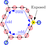
(A)	(B)	(C)

If the signal arrives on two of the three wires, then again, one of the points must be exposed. It is easy to verify that in any of these cases, there is a portion of the clause between two gates that needs covering, but it contains an odd number of points – thus the points can not be covered with disks of radius one.

If the signal arrives on all three wires then the points of the clause can not be covered, by the same argumentation of case (B) above (for the reader’s enjoyment, we show a different covering pattern in the figure).

Figure 7: The clause gadget can be satisfied iff the signal arrives on only one wire.

References

- [AGK+01] V. Arya, N. Garg, R. Khandekar, K. Munagala, and V. Pandit. Local search heuristic for -median and facility location problems. In Proc. 33rd Annu. ACM Sympos. Theory Comput., pages 21–29, 2001.
- [AMR11] D. Arthur, B. Manthey, and H. Röglin. Smoothed analysis of the -means method. J. Assoc. Comput. Mach., 58(5):19:1–19:31, 2011.
- [APF+10] G. Aggarwal, R. Panigrahy, T. Feder, D. Thomas, K. Kenthapadi, S. Khuller, and A. Zhu. Achieving anonymity via clustering. ACM Transactions on Algorithms, 6(3), 2010. A preliminary version of this paper appeared in PODS 2006.
- [ARR98] S. Arora, P. Raghavan, and S. Rao. Approximation schemes for Euclidean -median and related problems. In Proc. 30th Annu. ACM Sympos. Theory Comput., pages 106–113, 1998.
- [AS11] S. Ahmadian and C. Swamy. Improved approximation guarantees for lower-bounded facility location. CoRR, abs/1104.3128, 2011.
- [CGTS99] M. Charikar, S. Guha, E. Tardos, and D. B. Shmoys. A constant-factor approximation algorithm for the -median problem. In Proc. 31st Annu. ACM Sympos. Theory Comput., pages 1–10, 1999.
- [Cha01] T. Chan. On enumerating and selecting distances. Int. J. Comput. Geometry Appl., 11(3):291–304, 2001.
- [Che06] K. Chen. On -median clustering in high dimensions. In Proc. 17th ACM-SIAM Sympos. Discrete Algorithms, pages 1177–1185, 2006.
- [Che08] K. Chen. A constant factor approximation algorithm for -median clustering with outliers. In Proc. 19th ACM-SIAM Sympos. Discrete Algorithms, pages 826–835, 2008.
- [CK95] P. B. Callahan and S. R. Kosaraju. A decomposition of multidimensional point sets with applications to -nearest-neighbors and -body potential fields. J. Assoc. Comput. Mach., 42:67–90, 1995.
- [DHS01] R. O. Duda, P. E. Hart, and D. G. Stork. Pattern Classification. Wiley-Interscience, New York, 2nd edition, 2001.
- [DHW12] A. Driemel, S. Har-Peled, and C. Wenk. Approximating the Fréchet distance for realistic curves in near linear time. Discrete Comput. Geom., 48:94–127, 2012.
- [FG88] T. Feder and D. H. Greene. Optimal algorithms for approximate clustering. In Proc. 20th Annu. ACM Sympos. Theory Comput., pages 434–444, 1988.
- [Gon85] T. Gonzalez. Clustering to minimize the maximum intercluster distance. Theoret. Comput. Sci., 38:293–306, 1985.
- [Har04] S. Har-Peled. Clustering motion. Discrete Comput. Geom., 31(4):545–565, 2004.
- [Har11] S. Har-Peled. Geometric Approximation Algorithms. Amer. Math. Soc., 2011.
- [HK07] S. Har-Peled and A. Kushal. Smaller coresets for -median and -means clustering. Discrete Comput. Geom., 37(1):3–19, 2007.
- [HM06] S. Har-Peled and M. Mendel. Fast construction of nets in low dimensional metrics, and their applications. SIAM J. Comput., 35(5):1148–1184, 2006.
- [HR13] S. Har-Peled and B. Raichel. Net and prune: A linear time algorithm for euclidean distance problems. In Proc. 45th Annu. ACM Sympos. Theory Comput., 2013. To appear.
- [HS05] S. Har-Peled and B. Sadri. How fast is the -means method? Algorithmica, 41(3):185–202, January 2005.
- [KMN+04] T. Kanungo, D. M. Mount, N. S. Netanyahu, C. D. Piatko, R. Silverman, and A. Y. Wu. A local search approximation algorithm for -means clustering. Comput. Geom. Theory Appl., 28:89–112, 2004.
- [KSS10] A. Kumar, Y. Sabharwal, and S. Sen. Linear-time approximation schemes for clustering problems in any dimensions. J. Assoc. Comput. Mach., 57(2), 2010.
- [Llo82] S. Lloyd. Least squares quantization in pcm. IEEE Transactions on Information Theory, 28:129–137, 1982.
- [MR08] W. Mulzer and G. Rote. Minimum-weight triangulation is np-hard. J. ACM, 55(2), 2008.
- [Svi10] Z. Svitkina. Lower-bounded facility location. ACM Transactions on Algorithms, 6(4), 2010.