Three-tier CFTs from Frobenius algebras

Abstract.

These are lecture notes of a course given at the Summer School on Topology and Field Theories held at the Centre for Mathematics of the University of Notre Dame, Indiana, from May 29 to June 2, 2012.

The idea of extending quantum field theories to manifolds of lower dimension was first proposed by Dan Freed in the nineties. In the case of conformal field theory (cft), we are talking of an extension of the Atiyah-Segal axioms, where one replaces the bordism category of Riemann surfaces by a suitable bordism bicategory, whose objects are points, whose morphism are 1-manifolds, and whose 2-morphisms are pieces of Riemann surface.

There is a beautiful classification of full (rational) cft due to Fuchs, Runkel and Schweigert, which roughly says the following. Fix a chiral algebra $A$ (= vertex algebra). Then the set of full cfts whose left and right chiral algebras agree with $A$ is classified by Frobenius algebras internal to $\text{Rep}\,(A)$. A famous example to which one can successfully apply this is the case where the chiral algebra $A$ is affine $\mathfrak{su}(2)$ at level $k$, for some $k\in\mathbb{N}$. In that case, the Frobenius algebras in $\text{Rep}\,(A)$ are classified by $A_{n}$, $D_{n}$, $E_{6}$, $E_{7}$, $E_{8}$, and so are the corresponding cfts.

Recently, Kapustin and Saulina gave a conceptual interpretation of the FRS classification in terms of 3-dimensional Chern-Simons theory with defects. Those defects are also given by Frobenius algebra object in $\text{Rep}\,(A)$. Inspired by the proposal of Kapustin and Saulina, we will (partially) construct the three-tier cft associated to a Frobenius algebra object.

1. Introduction

In these notes we define, and partially construct, extended conformal field theories starting from a so-called chiral conformal field theory, and a Frobenius algebra object.

The idea of extended field theory, which goes back to the work of Freed in the ninetees [Fre93], started in the context of topological field theory. There, it is an extension of Atiyah’s definition of topological quantum field theory (tqft) [Ati89] where, instead of just assigning vector spaces to $(d-1)$-dimensional manifolds and linear maps to $d$-dimensional cobordisms, one also assigns data to manifolds of lower dimension, all the way down to points. Thus, the extended field theory consists of $d+1$ tiers.

Extended conformal field theories (cfts) were first proposed by Stolz and Teichner [ST04], in the context of their project of constructing elliptic cohomology, and then also mentioned in a review paper by Segal [Seg07]. However, they did not provide any constructions of extended cfts. We will show that this can be done, at least to a great extent.

1.1. Outline

Let us briefly outline the content of these notes. In Section 2 we introduce (full) cft in the formalism of Graeme Segal, and define extended cft. The source and target bicategories of extended cft are discussed in some detail.

Section 3 contains a discussion of chiral cfts. We introduce the two important ingredients of our construction: conformal nets, and Frobenius algebra objects. We also recall some aspects of the construction of Fuchs, Runkel and Schweigert, which constructs a (non-extended) full cft from a chiral cft and a Frobenius algebra object in the associated category.

In Section 4 we describe work in progress: the construction of an extended cft from a conformal net, and a Frobenius algebra object in the representation category of the conformal net. We finish by describing the main unsolved problem, namely the construction of the bimodule map that corresponds to a surface with four cusps (the ‘ninja star’ in Figure 1). If this could be done, this would complete the construction of the full cft.

Figure 1. A ‘ninja star’ is a 2-surface with four cusps. Our main open problem is to construct the corresponding map of bimodules.

2. Extended conformal field theory

The definition of extended cft is an extension of Segal’s definition of cft. We start at the beginning, and introduce cft in Segal’s formalism. We will also discuss the notion of conformal welding, which is a necessary ingredient of the definition.

2.1. Segal’s definition of conformal field theory

There are several (non-equivalent) ways to define conformal field theory. Although Segal’s definition [Seg88, Seg04] is not the most mainstream one, it is the one that has become popular amongst mathematicians.

Definition (Segal).

A full conformal field theory is a symmetric monoidal functor from the category of conformal cobordisms, which consists of

$$\begin{cases}\ \text{objects: one-dimensional, compact, oriented, smooth manifolds;}\\ \ \text{morphisms: cobordisms equipped with a complex structure;}\\ \ \text{monoidal structure: taking disjoint unions;}\end{cases}$$

to the category of Hilbert spaces, with

$$\begin{cases}\ \text{objects: Hilbert spaces;}\\ \ \text{morphisms: bounded linear maps;}\\ \ \text{monoidal structure: usual tensor product of Hilbert spaces.}\end{cases}$$

Let us take a closer look at the category of conformal cobordisms. Its objects consist of possibly empty disjoint unions of oriented circles (no parametrizations), always with a smooth structure. A cft maps a circle to a Hilbert space, referred to as the ‘state space’ by physicists, and a diffeomorphisms between circles to a unitary isomorphism. It then maps the disjoint unions of $k$ circles to the tensor product of the Hilbert spaces associated to the individual circles. Finally, the empty manifold, which is the unit object for the monoidal structure, is sent to the trivial Hilbert space $\mathbb{C}$, which is the unit for the tensor product in the category of Hilbert spaces.

The morphisms are Riemann surfaces with boundary. Both the smooth structure and the complex structure extend all the way to the boundary of the cobordisms. Alternatively, one could take the complex structure to only be defined on the interior, and require that the cobordism be locally isomorphic to the upper half plane. The orientations of the one-manifolds have to be compatible with those of the cobordisms connecting them: if $\Sigma$ is a cobordism from $S$ to $S^{\prime}$, then by definition there exists an orientation preserving diffeomorphism from the boundary $\partial\Sigma$ of $\Sigma$ to the disjoint union $S\amalg\overline{S^{\prime}}$ of the ‘ingoing’ manifold $S$ and the ‘outgoing’ $S^{\prime}$ with orientation reversed.

A cft sends cobordisms to linear maps between Hilbert spaces, the ‘propagator’ or ‘correlator’. In particular, a closed cobordism $\Sigma$ between two empty manifolds is mapped to a linear map $\mathbb{C}\longrightarrow\mathbb{C}$. The latter is completely determined by a single complex number $Z(\Sigma)$, the ‘partition function’ at the Riemann surface. A priori, the category of conformal cobordisms does not come with identity morphisms: those need to be added by hand, and one can then think of them as infinitesimally thin cobordisms. One also needs to include diffeomorphisms between 1-manifolds as degenerate cases of conformal cobordisms. More interesting is to go one step further and allow for cobordisms that are partially thin, and partially thick, such as the one in Figure 2.

Figure 2. A partially thin annulus.

Finally, the operator a cft associates to a morphism in the bordism category should depend continuously on the morphism. What this means is somewhat involved to explain, as it involves constructing a topology on the moduli space of all morphisms, encompassing honest bordisms and diffeomorphisms. More precisely, the dependence should be real-analytic in the interior of the moduli space (honest bordisms), and continuous on the boundary (diffeomorphisms).

2.1.1. Conformal welding

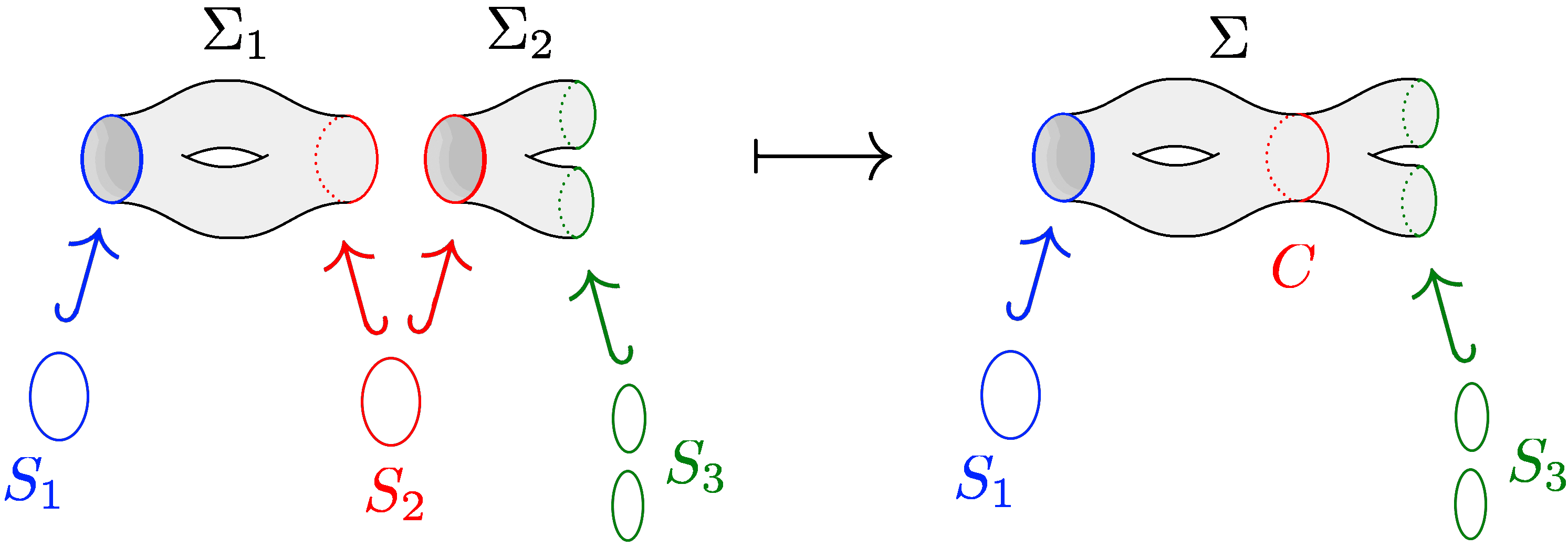
Figure 3. Conformal welding of two composable cobordisms.

The composition of conformal cobordisms is tricky and deserves special attention. We outline the procedure, which is called conformal welding. Consider two composable cobordisms $\Sigma_{1}$ and $\Sigma_{2}$ as depicted in Figure 3. As topological spaces, $\Sigma_{1}$ and $\Sigma_{2}$ can be glued in the obvious way. However, a priori, the composition $\Sigma$ is only equipped with a smooth structure away from the curve $C$ along which $\Sigma_{1}$ and $\Sigma_{2}$ have been glued, and similarly for the complex structure. These issues are resolved by the following theorem [Seg, RS06].

Theorem 2.1.

In the above situation, there exists a unique complex structure on the interior of the topological manifold $\Sigma$ which is compatible with the given complex structures on $\Sigma_{1}$ and $\Sigma_{2}$. Moreover, the embedding of $C$ into $\Sigma$ is smooth.

Note that the embedding $C\hookrightarrow\Sigma$ will typically not be analytic; this already signals that the proof of the theorem will have to be rather involved. A closely related result, which is needed in the proof that conformal welding is well defined, is [Bel90]:

Lemma 2.2.

Let $D\subset\mathbb{C}$ be a connected, simply connected open subset of the complex plane, and let us assume that the boundary of $D$ is smooth. Let $D_{0}\subset\mathbb{C}$ be the standard disc centered at the origin. Then the map $D\longrightarrow D_{0}$ provided by the Riemann mapping theorem is smooth all the way to the boundary.

Since the problem in Theorem 2.1 is local, one can reduce the general problem of conformal welding to the simpler situation of glueing two discs along a smooth identification of their boundaries. Moreover, using Lemma 2.2, one can further reduce the problem to that of glueing two standard discs along a smooth identification of their boundaries. Theorem 2.1 is therefore equivalent to the following special case of the theorem: given two standard discs $D_{0}$ and $D_{0}^{\prime}$ in $\mathbb{C}$, and a diffeomorphism $\varphi$ between their boundaries, the resulting glued surface is a copy of the Riemann sphere $\mathbb{CP}^{1}$, along with a smoothly embedded curve in it, as shown in Figure 4.

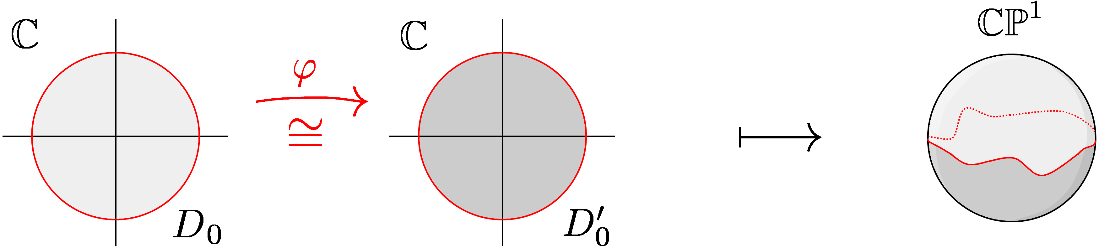
Figure 4. Glueing two standard discs along their boundaries results in the Riemann sphere with a smoothly embedded curve.

In order to get an extended cft, both the source and target categories in Segal’s definition of a cft are replaced by appropriate bicategories. An extended cft is then simply a symmetric monoidal functor between these bicategories. We first discuss the source bicategory.

2.2. The source bicategory: conformal surfaces with cusps

Geometrically, an extended cobordism is a cobordism, say $d$-dimensional, whose boundary comes in two pieces where each piece is viewed as $(d-1)$-dimensional cobordisms, and so on. In the case of cfts one is interested in $d=2$, resulting in three tiers: zero-manifolds, one-manifolds, and two-manifolds.

The source category is therefore not a category but rather a bicategory, see [Ben67] for background and definitions. Before describing this bicategory in more detail, let us give the geometrical picture. Starting in dimension zero, we first have zero-dimensional, oriented manifolds: these are disjoint unions of points, each of which is labelled $+$ or $-$ indicating the orientation. Moving up one dimension, we have cobordisms between the zero-dimensional manifolds.

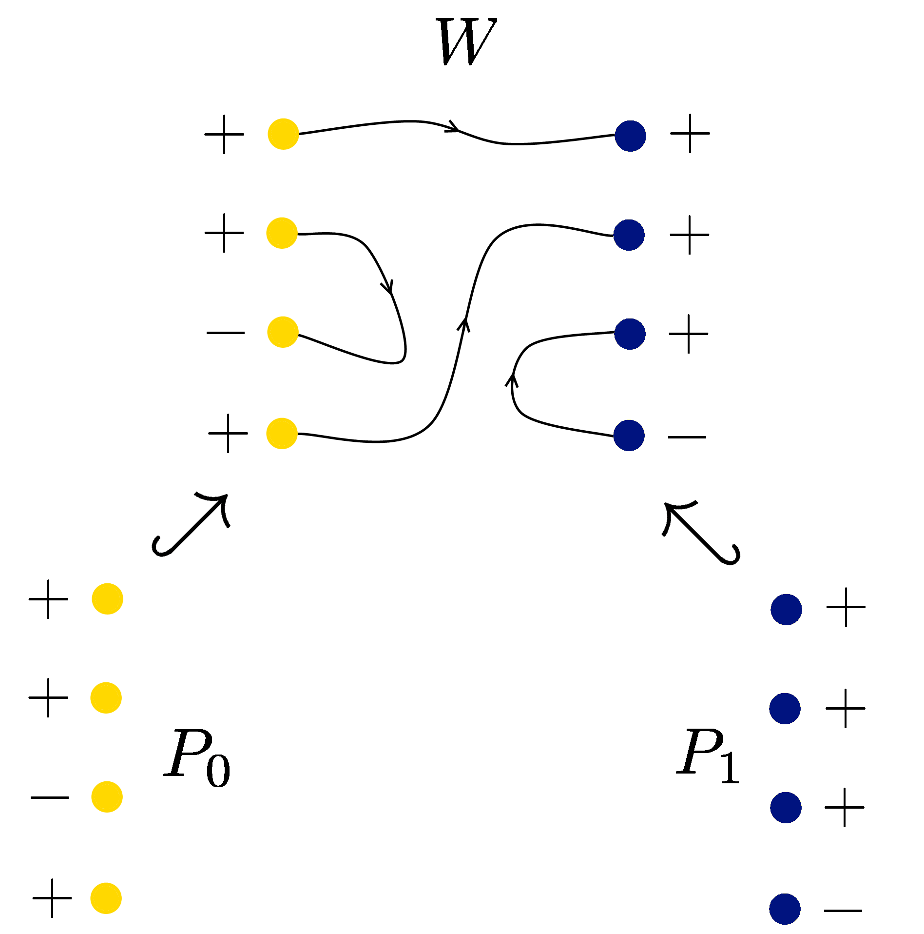
(a) An example of a one-dimensional cobordism $W\colon P_{0}\longrightarrow P_{1}$.

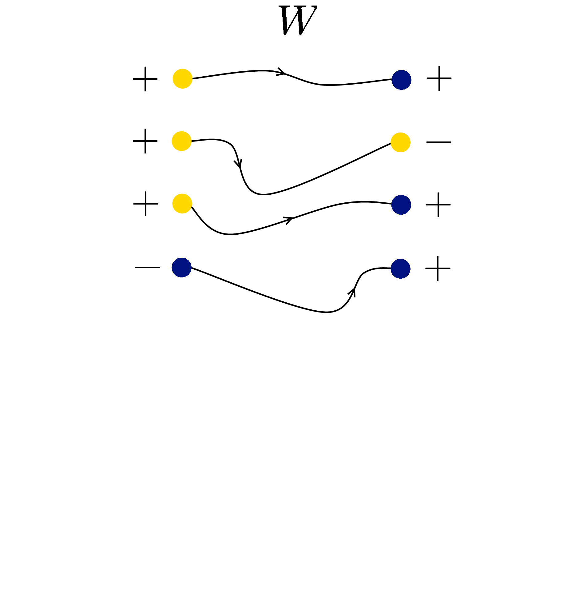
(b) The same cobordism, depicted in a more convenient way.

Figure 5. The figure on the left shows a one-dimensional cobordism. Notice that the orientation of the points is related to the orientation of the cobordisms connecting them, as required by the definition of a cobordism. The figure on the right shows the same cobordism displayed in way that will be more suitable for illustrations of two-dimensional cobordisms: the incoming and outgoing zero-manifold are distinguished by their color, and the inclusion of the boundary manifolds is understood.

An example of such a one-dimensional cobordism shown in Figure 5(a), all ‘incoming’ zero-manifolds are on the left, and all ‘outgoing’ on the right. To facilitate drawing the more complicated examples below it is convenient to employ a different convention, and use colors to represent whether a zero-manifold is incoming or outgoing, respectively. With this convention, the example from Figure 5(a) can also be represented as in Figure 5(b).

Circles, which form the objects of the source category of a non-extended cft, fit in the formalism of extended cft as closed cobordisms between empty zero-manifolds. They can be obtained from intervals by glueing. Going up one more dimension, cobordisms between such closed cobordisms are the conformal cobordisms that we encountered before: these are Riemann surfaces with boundary. However, now we also have two-dimensional cobordisms with cusps such as the examples in Figure 6.

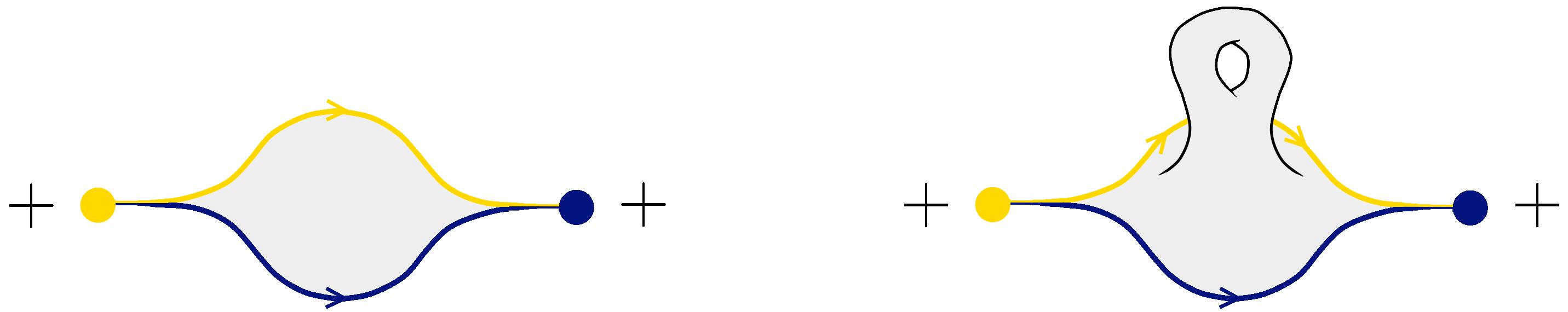
Figure 6. Two examples of two-dimensional cobordisms with cusps. The cobordism on the right has a nontrivial topology. Like in Figure 5(b), the colors indicate which one-dimensional boundary is incoming and which is outgoing.

The source category is the bicategory of conformal surfaces with cusps, which is defined as follows. It has

• objects: zero-dimensional, oriented manifolds $P$.

• 1-morphisms: one-dimensional cobordisms $P_{0}\hookrightarrow W\hookleftarrow P_{1}$ with smooth structure, and collars $P_{0}\times[\,0,\varepsilon)\longrightarrow W$ and $P_{1}\times(-\varepsilon,0\,]\longrightarrow W$ parametrizing the ends.

• 2-morphisms: two-dimensional cobordisms $W_{0}\hookrightarrow\Sigma\hookleftarrow W_{1}$ of cobordisms, with conformal structure in the interior $\Sigma\setminus(W_{0}\cup W_{1})$, and such that the diagrams

        and      

  commute, after maybe shrinking $\varepsilon$. Furthermore, $\Sigma$ should be locally isomorphic to one of the local models specified in Section 2.2.1 below.

The two diagrams above say that the parametrizations of the one-dimensional cobordisms bounding the surface have to agree on neighbourhoods of their ends. In particular, this forces the two-dimensional cobordism $\Sigma$ to be in fact one-dimensional near the zero-manifolds $P_{0}$ and $P_{1}$. Figure 7 shows an example of a 2-morphism in the category of conformal surfaces with cusps. Taking disjoint unions endows the category of conformal surfaces with cusps with a symmetric monoidal structure.

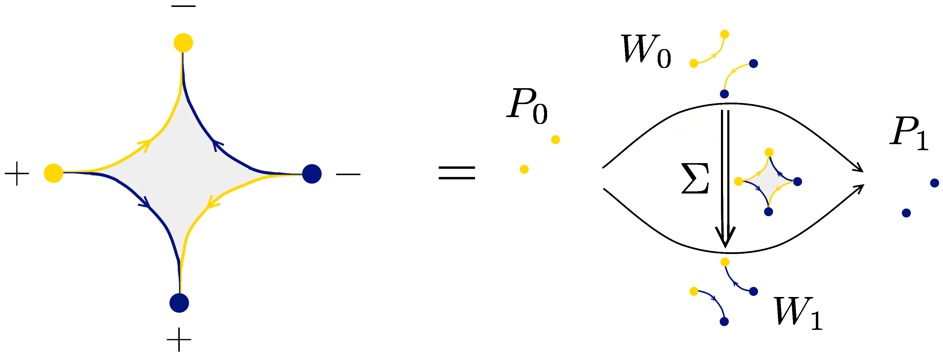
Figure 7. An example of a conformal surface with cusps, and the corresponding 2-morphism $\Sigma\colon W_{0}\longrightarrow W_{1}$.

2.2.1. Local models

The various manifolds comprising the bicategory of conformal surfaces admit local models. Being a local model means that any point of such a manifold has a neighbourhood that looks the same as some open subset of the corresponding local model. For example, the local model of an object $P$ is simply a point with a choice of orientation, and for a 1-morphism $S$ it is the unit interval $[0,1]$. Unlike for the case of 0-morphisms (objects) and 1-morphisms, where one can show that, locally, they must look like one of the local models, the case of 2-morphisms is different. For 2-morphisms, giving the list of allowed local models is part of the definition of what things we allow as 2-morphisms.

We can describe the local models for our 2-morphisms $\Sigma$ as follows. Let $f,g\in C^{\infty}\big{(}[0,1],\mathbb{R}\big{)}$ be smooth functions on the unit interval, such that $f\leq g$, and such that $f$ and $g$ are equal on neighbourhoods of $0$ and $1$. Then a local model of $\Sigma$ is

(1) $$\Sigma=\{\,x+i\,y\mid f(x)\leq y\leq g(x)\,\}\ .$$

In particular, since we require $f$ and $g$ to agree near the ends, the tips of $\Sigma$ are really one-dimensional cusps as depicted in Figure 8. There are many different local models for the 2-morphisms, with different choices for $f$ and $g$ yielding varying degrees of ‘sharpness’ for the cusps.

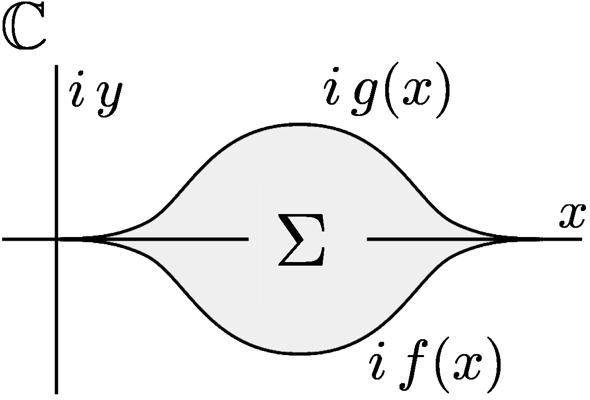
Figure 8. A local model as described by equation (1). Different choices for $f,g\in C^{\infty}\big{(}[0,1],\mathbb{R}\big{)}$ agreeing near the endpoints give rise to different degrees of sharpness for the cusps.

Since the 1-morphisms correspond to collared one-manifolds, they can be composed by glueing. To see that the glued surfaces with cusps are again of the prescribed form, notice that our problem is local. Thus we may assume without loss of generality that the surfaces we want to glue are given by the local models. It is clear from Figure 9 that the horizontal composition is again of the form (1).

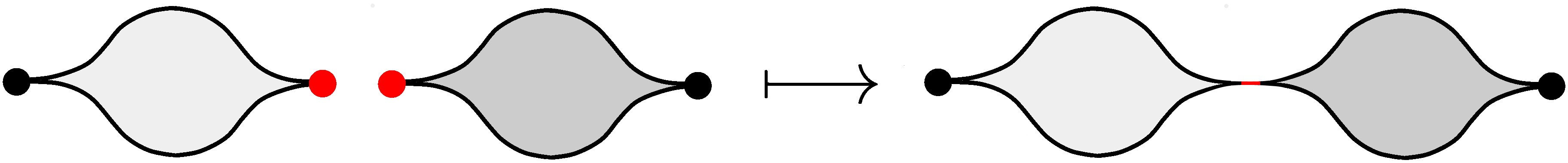
Figure 9. Horizontal composition of two-dimensional local models.

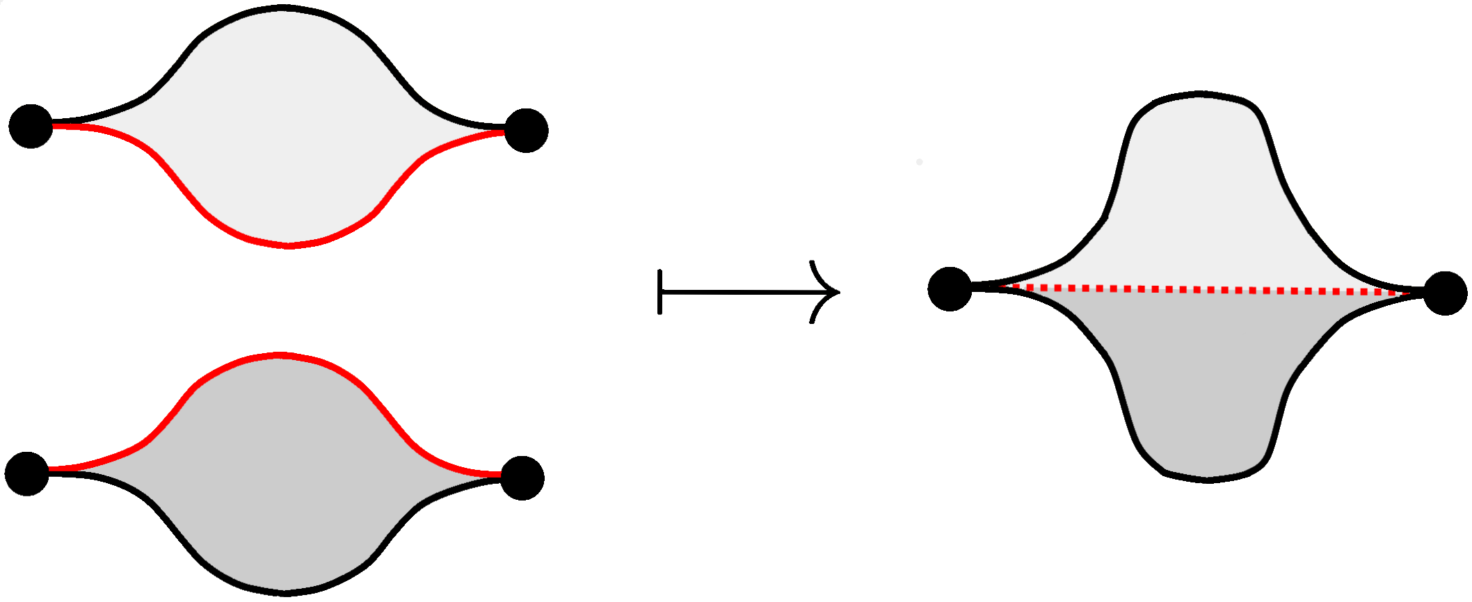
Figure 10. Vertical composition of two local models for conformal surfaces with cusps. It requires some work to show that the result is a local model too.

The vertical composition of two 2-morphisms looks as shown in Figure 10. We can use Theorem 2.1, underlying conformal welding, to get a complex structure on the interior of the glued surface. But a priori, it is not clear that the result is again one of our local models. To show that, we will use Lemma 2.2. First we get rid of the corners by embedding the two surfaces that we want to glue into discs with a smooth boundary, as shown in Figure 11. Next, we extend the diffeomorphism of the boundaries of the surfaces that we want to identify to a diffeomorphism between the boundary circles, and glue. The result is depicted in Figure 12. By Lemma 2.2, everything is smoothly embedded in $\mathbb{CP}^{1}$. This shows that the glued surface is again one of our allowed local models, and so it is again a 2-morphism.

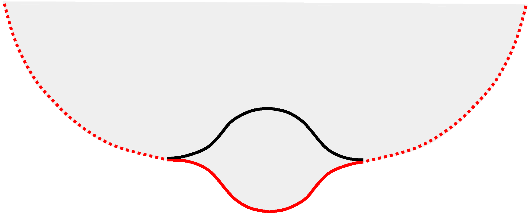
Figure 11. A local model $\Sigma$ can be embedded into some disc whith smooth boundary in the complex plane.

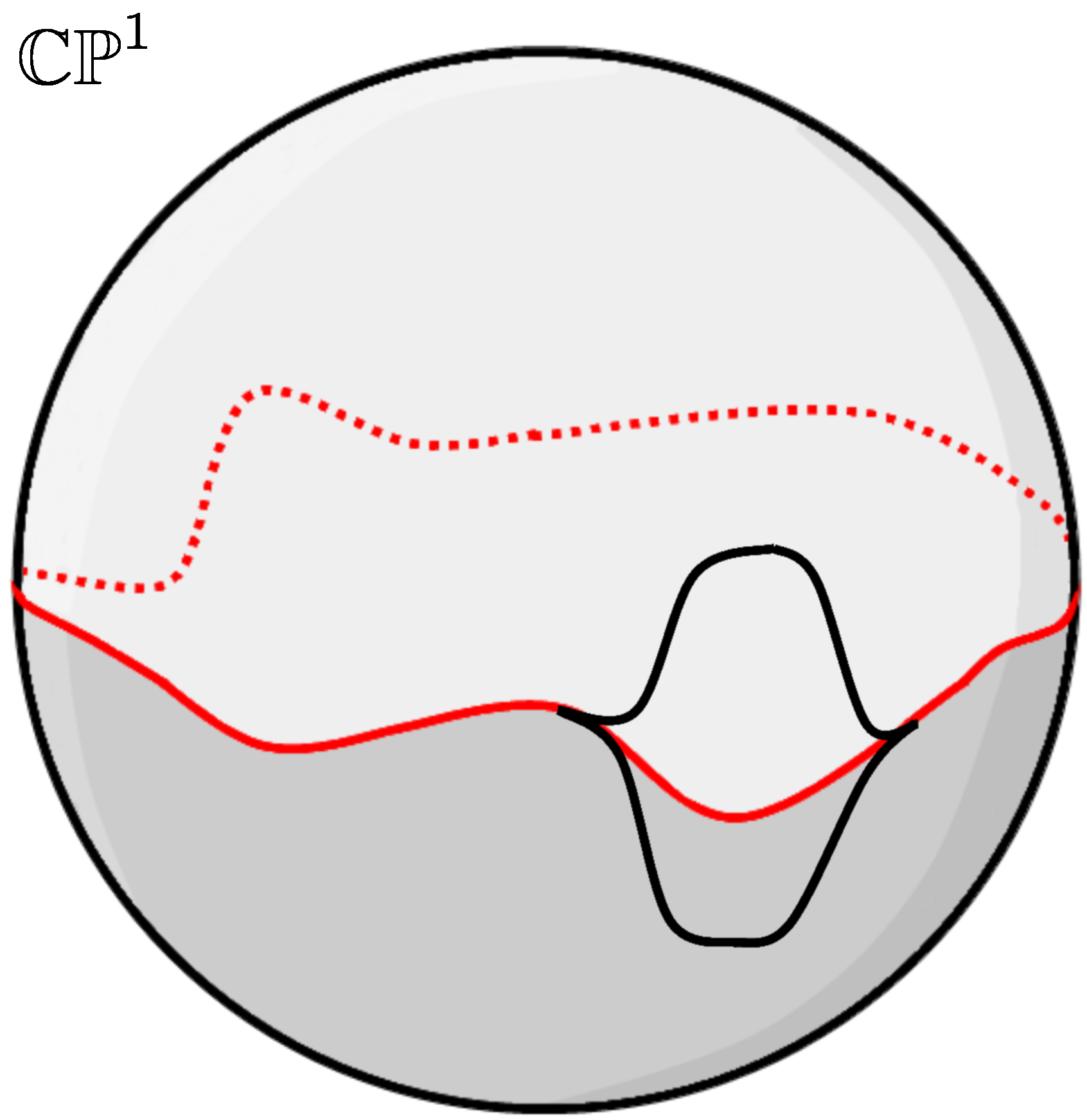
Figure 12. Glueing two local models $\Sigma_{1}$ and $\Sigma_{2}$ that are embedded into discs like in Figure 11 yields a copy of the vertical composition of $\Sigma_{1}$ and $\Sigma_{2}$ inside the Riemann sphere.

2.3. The target bicategory: von Neumann algebras

Since an extended cft should encompass the notion of cft, it should certainly map (a union of) circles to some Hilbert space, and a cobordism connecting such circles to a linear map between Hilbert spaces, as before. We have to decide what we want to assign to a point: these should be some kind of algebras. If we want to stay in a Hilbert space setting, then there are not many options for the kind of algebras to consider. It turns out that the appropriate choice is given by von Neumann algebras. A one-dimensional cobordism is then mapped to a bimodule between von Neumann algebras, and a surface such as (1) corresponds to a linear map between bimodules. In short, the target bicategory is defined as follows:

• objects: von Neumann algebras;

• 1-morphisms: bimodules (that is, Hilbert spaces with a left action of the first von Neumann algebra, and a commuting right action of the second von Neumann algebra);

• 2-morphisms: bounded linear maps that are compatible with the bimodule structure.

Before we give a definition of these notions, we recollect some facts from the theory of operator algebras. Given a Hilbert space $H$, denote the algebra of bounded operators on $H$ by $B(H)$. Recall that an operator $a\in B(H)$ is trace class if it is compact and the trace-norm $\|a\|_{1}\coloneqq\sum_{k}\sqrt{\mu_{k}}$ is finite; here the $\mu_{k}$ are the eigenvalues of the positive operator $a^{*}a$. This ensures that the trace of $a$ is well defined. Write $B_{1}(H)$ for the trace-class operators in $B(H)$. The pairing

$$B(H)\times B_{1}(H)\longrightarrow\mathbb{C}\ ,\quad(a,b)\longmapsto\text{tr}\,(a\,b)$$

induces a topology on $B(H)$ that is called the ultraweak topology. Thus, a (generalized) sequence $\{a_{i}\}$ in $B(H)$ converges ultraweakly to $a\in B(H)$ if and only if for all $b\in B_{1}(H)$ we have that $\text{tr}(a_{i}b)\longrightarrow\text{tr}(ab)$ in $\mathbb{C}$.

Definition.

A von Neumann algebra is a topological $*$-algebra $A$ over $\mathbb{C}$ that can be embedded in some $B(H)$ as a ultraweakly closed $*$-subalgebra.

By the von Neumann bicommutant theorem, $A$ is ultraweakly closed if and only if it is its own bicommutant.

Definitions.

A module over a von Neumann algebra $A$ is a Hilbert space $H$ together with a continuous $*$-homomorphism $A\longrightarrow B(H)$.

Similarly, if $A$ and $B$ are von Neumann algebras, an $A$-$B$-bimodule is a Hilbert space $H$ equipped with two continuous $*$-homomorphisms $A\longrightarrow B(H)$ and $B^{\text{op}}\longrightarrow B(H)$ whose images commute. We write ${}_{A}M_{B}$ to indicate that $M$ is an $A$-$B$-bimodule.

Here we have written $B^{\text{op}}$ for the von Neumann algebra obtained from $B$ by reversing the order in the multiplication: if $m\colon B\otimes B\longrightarrow B$ is the original multiplication on $B$ then the opposite multiplication is given by $m^{\text{op}}(a,b)=b\,a$.

It is more work to define the composition of bimodules in the bicategory of von Neumann algebras than it is to do so in the bicategory of rings. Recall the way in which rings and bimodules form a bicategory. Given two rings $R$ and $S$, let $\text{Hom}(R,S)$ be the category of $R$-$S$-bimodules. The morphisms in $\text{Hom}(R,S)$ are then the 2-morphisms of our bicategory. If $R$, $S$, $T$ are rings, the horizontal composition of two bimodules ${}_{R}M_{S}$ and ${}_{S}N_{T}$ is given by the tensor product:

$${}_{A}M_{B}\circ{}_{B}N_{C}\coloneqq{}_{A}M\underset{B}{\otimes}N_{C}\ .$$

Here the tensor product is taken over $B$, so that $(m\cdot b)\otimes n=m\otimes(b\cdot n)$. The $A$-$A$-bimodule $A$ is then the unit object for this kind of composition.

If we want to do something similar with von Neumann algebras, the first obstacle is the definition of the unit object: a von Neumann algebra is not a Hilbert space, so it cannot serve as a bimodule over itself. However, there is a canonical way to turn a von Neumann algebra $A$ into a Hilbert space, called $L^{2}A$.

2.3.1. The $L^{2}$-space of a von Neumann algebra

The definition of $L^{2}A$ requires more prerequisites from the theory of operator algebras. We outline its construction.

For $A$ a von Neumann algebra, let

$$L^{1}A \coloneqq\{\ \varphi\colon A\longrightarrow\mathbb{C}\mid\text{continuous}\ \}\ ,$$

$$L^{1}_{+}A \coloneqq\{\ \varphi\in L^{1}A\mid\varphi(a^{*}a)\geq 0\ \text{for all}\ a\in A\ \}\ .$$

Elements of $L^{1}_{+}A$ are called states on $A$. The Gelfand-Naimark-Segal construction says that for each state $\varphi\in L^{1}_{+}A$ there exists a cyclic representation $\pi_{\varphi}$ of $A$ on some Hilbert space $H_{\varphi}$ with cyclic vector $\Omega_{\varphi}$. Thus, the image $\pi_{\varphi}(A)\,\Omega_{\varphi}$ of the action of $A$ on $\Omega_{\varphi}$ is dense in $H_{\varphi}$.

If the state is faithful (i.e. if $\varphi(a^{*}a)>0$ for $a\not=0$), then the antilinear operator $\pi_{\varphi}(a)\,\Omega_{\varphi}\longmapsto\pi_{\varphi}(a)^{*}\,\Omega_{\varphi}$ defined on $\pi_{\varphi}(A)\,\Omega_{\varphi}$ can be extended to an operator $S_{\varphi}$ on the closure $H_{\varphi}$ of $\pi_{\varphi}(A)\,\Omega_{\varphi}$. From this operator we can further construct the positive operator $\Delta_{\varphi}\coloneqq|S_{\varphi}|^{2}=S_{\varphi}^{*}S_{\varphi}$. Since $\Delta_{\varphi}$ is a positive operator, $\Delta_{\varphi}^{it}=\exp(i\,t\log\Delta_{\varphi})$ is well defined for all $t\in\mathbb{R}$.

By a theorem that is due to Tomita and Takesaki, for each $a\in A$, the assignment $t\longmapsto\Delta_{\varphi}^{-it}\,a\,\Delta_{\varphi}^{it}$ defines a one-parameter family of elements in $A$. This is called the modular group of $A$ associated with $\varphi$.

Next, consider the algebra $\text{Mat}_{2}(A)$ of $2\times 2$ matrices with coefficients in $A$ and let $\varphi\oplus\psi\in L^{1}_{+}\big{(}\text{Mat}_{2}(A)\big{)}$. Via the above construction, $\varphi\oplus\psi$ yields a modular group in $\text{Mat}_{2}(A)$. Applying this modular group to the element

$$\left(\begin{array}[]{cc}0&1\\ 0&0\end{array}\right)\in\text{Mat}_{2}(A)$$

we get elements that are of the form

$$\Delta_{\varphi\oplus\psi}^{-it}\left(\begin{array}[]{cc}0&1\\ 0&0\end{array}\right)\Delta_{\varphi\oplus\psi}^{it}=\left(\begin{array}[]{cc}0&\cdots\\ 0&0\end{array}\right)\ \in\mathrm{Mat}_{2}(A)\,.$$

The non-commutative Radon-Nikodym derivative $[D\varphi:D\psi]_{t}$ is then defined via

$$\left(\begin{array}[]{cc}0&[D\varphi:D\psi]_{t}\\ 0&0\end{array}\right)\coloneqq\Delta_{\varphi\oplus\psi}^{-it}\left(\begin{array}[]{cc}0&1\\ 0&0\end{array}\right)\Delta_{\varphi\oplus\psi}^{it}\ .$$

Now consider the free vector space on symbols $\sqrt{\varphi}$ with $\varphi\in L^{1}_{+}A$. The above construction allows us to define a (semi-definite) inner product on this vector space via the formula

$$\langle\,\sqrt{\varphi},\sqrt{\psi}\,\rangle\coloneqq\operatorname*{anal.cont.}_{t\longrightarrow i/2}\,\varphi\big{(}[D\varphi:D\psi]_{t}\big{)}\ .$$

After all these preliminaries, we are finally in a position to define $L^{2}A$: it is the Hilbert space obtained as the completion of the above free vector space with respect to this inner product. For each von Neumann algebra $A$, the Hilbert space $L^{2}A$ is an $A$-$A$-bimodule, ${}_{A}L^{2}A_{A}$, and this is the unit morphism in the bicategory of von Neumann algebras.

The Hilbert space $L^{2}A$ is also equipped with a positive cone $L_{+}^{2}A\subset L^{2}A$, given by

$$L_{+}^{2}A:=\{\sqrt{\varphi}\,|\,\varphi\in L_{+}^{1}A\}\,,$$

and an antilinear involution $J:L^{2}A\to L^{2}A$, called the modular conjugation. The modular conjugation is given by $J(\sum_{i}c_{i}\sqrt{\varphi_{i}}):=\sum_{i}\bar{c}_{i}\sqrt{\varphi_{i}}$.

2.3.2. Connes fusion

The second difficulty towards defining the bicategory of von Neumann algebras is that the ordinary tensor product does not work: it would have ${}_{A}A_{A}$ as its unit, not ${}_{A}L^{2}(A)_{A}$. The appropriate tensor product of von Neumann bimodules, known as Connes fusion and denoted by $\boxtimes$, is tailor-made so that ${}_{A}L^{2}A_{A}$ is a unit for that operation. We have

(2) $$M\underset{A}{\boxtimes}N\coloneqq\text{completion of }M\underset{A}{\otimes}\text{Hom}_{A}(L^{2}A,N)\,.$$

This is actually forced on us if we want $L^{2}A$ to be the unit. If we accept for a moment that $L^{2}A$ is a unit, then given an $A$-linear map $\varphi\colon L^{2}A\longrightarrow N$ and an element $m\in M$, there is an easy way of producing an element of $M\boxtimes_{A}N$: take the image of $m\in M\cong M\boxtimes_{A}L^{2}A$ under the map $1\boxtimes\varphi:M\boxtimes_{A}L^{2}A\to M\boxtimes_{A}L^{2}N$.

The completion is taken with respect to an inner product on the right-hand side of (2). Let us work backwards to figure out the correct formula for the inner product. The inner product of two elements $n\otimes\phi$ and $m\otimes\psi$ of $M\boxtimes_{A}N$ can be described as the composition

where $\phi,\psi\in\text{Hom}_{A}(L^{2}A,N)$, $\psi^{*}$ is the adjoint of $\psi$, and we view $m,n\in M$ as maps $\mathbb{C}\longrightarrow M$. Notice that the map $\psi^{*}\circ\phi\colon{}_{A}L^{2}A\longrightarrow{}_{A}L^{2}A$ commutes with the left action of $A$ on $L^{2}A$. Now, one of the properties of $L^{2}A$ is that endomorphisms of $L^{2}A$ which are equivariant for the left $A$-action are given by right multiplication $\rho_{a}$ by some $a\in A$. Therefore we have that $\psi^{*}\circ\phi=\rho_{a}$ for some $a=a_{\psi^{*}\circ\phi}\in A$. The inner product $\langle m\otimes\phi,n\otimes\psi\rangle$ on $M\otimes\text{Hom}_{A}(L^{2}A,M)$ is now given by the composition

$$\vbox{\hbox{ \leavevmode\hbox to227.28pt{\vbox to19.87pt{\text{[drawing]}}}}}\,. \mathbb{C} M M \mathbb{C} \scriptstyle n \rho_{a} \scriptstyle m^{*} \mathbb{C} M M \mathbb{C} \scriptstyle n \rho_{a} \scriptstyle m^{*}$$

A more symmetric way to write the Connes fusion product is

$$M\underset{A}{\boxtimes}N\cong\text{Hom}_{A}(L^{2}A,M)\underset{A}{\otimes}L^{2}A\underset{A}{\otimes}\text{Hom}_{A}(L^{2}A,N)\,.$$

The evaluation map $\text{Hom}_{A}(L^{2}A,M)\otimes_{A}L^{2}A\longrightarrow M$ relates this description to the previous asymmetric definition: after completion those two descriptions become isomorphic to each other.

3. Conformal nets and Frobenius algebra objects

Before we push on, let us pause a moment to sketch the big picture. Actually, there are a couple of different things called ‘cft’; in particular, physics distinguishes between chiral and full cft. It is quite common to use ‘cft’ to refer to one of these things, but it may not always be clear from the context to which one. What we have been calling cft above are really full cfts. We abbreviate ‘chiral cft’ to ‘$\chi$cft’ so that we can continue to use ‘cft’ without further specification exclusively for ‘full cft’.

Chiral cfts can be seen as an intermediate step towards full cft. The distinction between chiral and full cft has its origin in physics. Now comes the mathematics to make things more complicated: there exist different mathematical formalisms to talk about $\chi$cft, and to talk about full cft. We have already discussed Segal’s formalism for full cft. Chiral cft can be described in the formalism of Segal as well, and there are also approaches using vertex operator algebras or conformal nets. Shortly we will present $\chi$cft in Segal’s formalism, and in Sections 3.2.1 and 3.3 we will also look at the approach via conformal nets.

Recall that the loop group of a compact Lie group $G$ is defined as the group of maps from the unit circle into $G$:

(3) $$L\,G\coloneqq\text{Map}_{C^{\infty}}(S^{1},G)\ .$$

Loop groups are relevant for us because they lead to vertex operator algebras or conformal nets, and so they provide examples of $\chi$cfts. In order to construct a full cft out of a $\chi$cft, one needs additional data: a Frobenius algebra object in the monoidal category associated to the $\chi$cft. In Section 3.4 we will define Frobenius algebra objects, and in Section 3.5 we will illustrate how such an object helps to construct a full cft out of a $\chi$cft.

To summarize, the situation can be represented as follows:

We will show that with the same input, a chiral cft and a Frobenius algebra object, one can actually do better and construct an extended cft:

(4)

In Section 4 we will (partially) construct examples of extended cfts. We should put this task into perspective: already for (non-extended) Segal cfts, the interesting examples — most notably those coming from loop groups — have not completely been constructed. In the spirit of the cobordism hypothesis [Lur09], one could even hope that it is easier to construct extended cfts than full cfts.

3.1. Chiral conformal field theory

In this section, we use Segal’s formalism to describe (non-extended) $\chi$cft. Recall from Section 2.1 that a non-extended cft assigns Hilbert spaces to closed one-dimensional manifolds, and maps between Hilbert spaces to conformal cobordisms. Chiral cfts have the same source category as full cfts, but there is an intermediate layer on the side of the target.

A $\chi$cft first assigns to every closed one-dimensional manifold a $\mathbb{C}$-linear category $\mathcal{C}$. To each object $\lambda\in\mathcal{C}$, it further assigns a Hilbert space $H_{\lambda}$. Likewise, a cobordism (always with complex structure) is mapped to a functor $f\colon\mathcal{C}_{\text{in}}\longrightarrow\mathcal{C}_{\text{out}}$, and for each $\lambda\in\mathcal{C}_{\text{in}}$ we further get a map $H_{\lambda}\longrightarrow H_{f(\lambda)}$. This is only part of the data of a $\chi$cft, but we can already try to list certain axioms. Most importantly, the map $H_{\lambda}\longrightarrow H_{f(\lambda)}$ must depend on the complex structure of the cobordism in a holomorphic fashion. Here is what this means, roughly. If we fix two one-manifolds $W_{\text{in}}$ and $W_{\text{out}}$, then the (infinite-dimensional) moduli space of Riemann surfaces with these boundaries has its own complex structure: the functions from this moduli space, mapping points to operators, are required to be holomorphic.

Note however that the Hilbert space $H_{f(\lambda)}$ depends on the choice of cobordism. So, as a prerequisite for the above condition to make sense, $f\colon\mathcal{C}_{\text{in}}\longrightarrow\mathcal{C}_{\text{out}}$ should depend holomorphically on the choice of cobordism. That is, the Hilbert spaces $H_{f(\lambda)}$ should form a holomorphic bundle over the moduli space of complex cobordisms. On top of that, there is also a unitary projectively flat connection on that same bundle: a path between two cobordisms (in the moduli space of cobordisms between $W_{\text{in}}$ and $W_{\text{out}}$) then induces a natural isomorphism between the corresponding functors, and if two paths are homotopic, then the two natural isomorphisms are equal up to a phase. So, overall, a $\chi$cft is a rather involved kind of structure.

To get a feeling about what these categories associated to one-manifolds are, we look at the examples of $\chi$cfts which are provided by loop groups. Let $G$ be a Lie group. To a one-manifold $W$ in the source category we assign the category of representations of $\text{Map}_{C^{\infty}}(W,G)$ (compare with (3)). Moreover, each object $\lambda$ in that category has an underlying Hilbert space: those are the $H_{\lambda}$.

We should point out that $\chi$cft in the above formalism are difficult to construct, and despite a lot of hard work ([TUY89, Zhu96, Hua97, Pos03], and of course [Seg88]) the $\chi$cfts corresponding to loop groups have been constructed to a great extent, but not completely.

We finish our short discussion of chiral conformal field theories by emphasizing the most important structure that a such a theory encodes: a braided monoidal category. Let $\mathcal{C}$ be the category that the $\chi$cft assigns to the standard circle. Then the pair of pants equips $\mathcal{C}$ with a monoidal structure, and the diffeomorphism that switches the two pant legs (followed by a path inside the space of complex structures on the pair of pants) further equips it with the structure of a braided monoidal category.

3.2. Conformal nets

Our construction, as indicated in (4), is not based on the above formalism. Rather, it uses the formalism of conformal nets. To get acquainted with conformal nets we will start by giving the data of a conformal net and look at an example. In Section 3.3 we will give the complete abstract definition of conformal nets, including the axioms for the above data.

Data.

A conformal net $\mathcal{A}$ is a monoidal functor from the category

$$\begin{cases}\ \text{objects: compact, oriented, one-dimensional manifolds with boundary;}\\ \ \text{morphisms: embeddings that either preserve the orientation on all}\\ \ \qquad\qquad\text{connected components or reverse the orientation everywhere}\end{cases}$$

to the category

$$\begin{cases}\ \text{objects: von Neumann algebras;}\\ \ \text{morphisms: injective homomorphisms and antihomomorphisms.}\end{cases}$$

We require that an embedding $W_{1}\hookrightarrow W_{2}$ is sent to an injective homomorphism $\mathcal{A}(W_{1})\rightarrow\mathcal{A}(W_{2})$ if it preserves orientation, and to an injective homomorphism $\mathcal{A}(W_{1})\rightarrow\mathcal{A}(W_{2})^{\text{op}}$ if it reverses orientation, where $\mathcal{A}(W_{2})^{\text{op}}$ is the opposite of the von Neumann algebra $\mathcal{A}(W_{2})$. (Note: an antihomomorphism $A\to B$ is a homomorphism $A\to B^{\text{op}}$).

3.2.1. Conformal nets associated to loop groups

An important class of examples of conformal nets is given by loop group nets. Let $G$ be a simply connected compact Lie group equipped with a ‘level’. If the group is simple, then a level is just a positive integer $k\in\mathbb{Z}_{\geq 1}$; in general, a level is a biinvariant metric on $G$ such that the square lengths of closed geodesics are in $2\mathbb{Z}$. To a one-manifold $W$ we want to assign an algebra. As an intermediate step towards this algebra, we define the group

(5) $$L_{W}G\coloneqq\text{Map}_{*}(W,G)\subset\text{Map}_{C^{\infty}}(W,G)$$

of all smooth maps $W\longrightarrow G$ that send the boundary $\partial W$ to the unit $e\in G$ and all of whose derivatives are zero at the boundary. Thus, if $W=S$ is a circle, then $L_{W}G$ is a version of the free loops on $G$, while if $W=I$ is an interval, it is a version of the based loops on $G$. The group structure is given by pointwise multiplication in $G$.

Like the loop group, this group has a central extension by $S^{1}$. That central extension is easiest to describe at the level of the Lie algebra $\mathfrak{g}$ of $G$, where it becomes a central extension by $\mathbb{R}$. The Lie algebra $L_{W}\mathfrak{g}$ of the loop group $L_{W}G$ consists of smooth maps $W\to\mathfrak{g}$ all of whose derivatives are zero at the boundary. It has a central extension defined by the cocycle

(6) $$c(f,g)=\int_{W}\langle\,f,\text{d}\,g\,\rangle_{k}\ ,\qquad f,g\in L_{W}\mathfrak{g}\ .$$

Here, the pairing is given by the metric and depends on the choice of level for $G$. The corresponding central extension of $L_{W}G$ is the one that we are after.

The value $\mathcal{A}(W)=\mathcal{A}_{LG,k}(W)$ of the conformal net $\mathcal{A}_{LG,k}$ on the 1-manifold $W$ is then defined as the completion of the group algebra of $L_{W}G$, with multiplication twisted by the cocycle (6). This is similar to the group algebra of the central extension, but the central $S^{1}$ is identified with the $S^{1}$ in the scalars. More precisely, we start by forming the free vector space $\mathbb{C}[L_{W}G]$; since $L_{W}G$ is a group, this free vector space has the structure of an algebra. The group cocycle $c\colon L_{W}G\times L_{W}G\longrightarrow\mathbb{C}^{*}$ corresponding to (6) allows us to modify the multiplication to $g\cdot_{c}h\coloneqq c(g,h)\,g\,h$. The associativity is maintained due to the cocycle condition $c(gh,k)\,c(g,h)=c(g,hk)\,c(h,k)$. Finally, the resulting twisted group algebra is not complete, and so we take some completion to make it into a von Neumann algebra.

Loop group nets are made so that they remember all the relevant information about the corresponding loop group. In particular, there is a notion of representation of a conformal net, and the representations of the loop group net agree with the ‘positive energy’ representation of $L\,G$.

Definition.

A representation of a conformal net $\mathcal{A}$ is a Hilbert space $H$ equipped with compatible actions of $\mathcal{A}(I)$ for every proper subinterval $I\subsetneq S^{1}$ of the unit circle. The category of representations of a conformal net $\mathcal{A}$ is denoted $\text{Rep}\,(\mathcal{A})$.

Note that although $S^{1}$ itself has a von Neumann algebra $\mathcal{A}(S^{1})$ associated to it, there are examples of conformal nets where $\mathcal{A}(S^{1})$ does not act on a representation $H$. For this reason, one requires actions of the algebras associated to all manifolds $I\subsetneq S^{1}$ that are strictly contained in $S$. Those must be compatible in the sense that the inclusions $I_{1}\hookrightarrow I_{2}\subset S^{1}$ determine the restrictions of the actions. Often, a representation is equivalent to having a single action of the algebra $\mathcal{A}(S^{1})$. We should expect this to hold for loop group nets in particular, although we do not know how this can be proven, except for $G=SU(n)$.

The category $\text{Rep}\,(\mathcal{A})$ is monoidal with respect to a product $\boxtimes$ called “fusion product”, which we now describe. Consider two representations $H$ and $K$ of $\mathcal{A}$, as shown in Figure 13. The two half-circles $I$ and $J$, with orientations induced by their inclusion in $S^{1}$, act as $\mathcal{A}(I)\hskip 2.84544pt{\begin{picture}(8.0,8.0)(0.0,0.0)\qbezier(7.0,6.0)(4.5,8.3)(2.0,7.0)\qbezier(2.0,7.0)(-1.5,4.0)(2.0,1.0)\qbezier(2.0,1.0)(4.5,-0.3)(7.0,2.0)\qbezier(7.0,6.0)(6.1,7.5)(6.8,9.0)\qbezier(7.0,6.0)(5.0,6.1)(4.2,4.4)\end{picture}\hskip 2.84544pt}H$ and $\mathcal{A}(J)\hskip 2.84544pt{\begin{picture}(8.0,8.0)(0.0,0.0)\qbezier(7.0,6.0)(4.5,8.3)(2.0,7.0)\qbezier(2.0,7.0)(-1.5,4.0)(2.0,1.0)\qbezier(2.0,1.0)(4.5,-0.3)(7.0,2.0)\qbezier(7.0,6.0)(6.1,7.5)(6.8,9.0)\qbezier(7.0,6.0)(5.0,6.1)(4.2,4.4)\end{picture}\hskip 2.84544pt}K$. Let $\varphi\colon I\longrightarrow J$ be the diffeomorphism that sends the ‘north pole’ to the ‘north pole’ and the ‘south pole’ to the ‘south pole’ (see again Figure 13). Since $\varphi$ reverses the orientation, it provides an isomorphism $\mathcal{A}(I)\cong\mathcal{A}(J)^{\text{op}}$ and therefore a right action of $\mathcal{A}(J)$ on $H$. The fusion product of $H$ and $K$ is then defined to be the Connes fusion $H\boxtimes_{\mathcal{A}(J)}K$. The residual actions of $S^{1}\setminus I$ and $S^{1}\setminus J$ can then be used to make this product into a new representation of $\mathcal{A}$. Moreover, one can show that, up to natural isomorphism, the functor $H,K\mapsto H\boxtimes_{\mathcal{A}(J)}K$ is independent of the choice of half-circles $I$ and $J$. This also shows that the category $\text{Rep}\,(\mathcal{A})$ is braided monoidal. The construction of these natural isomorphisms is spelled out in Section 3.3.

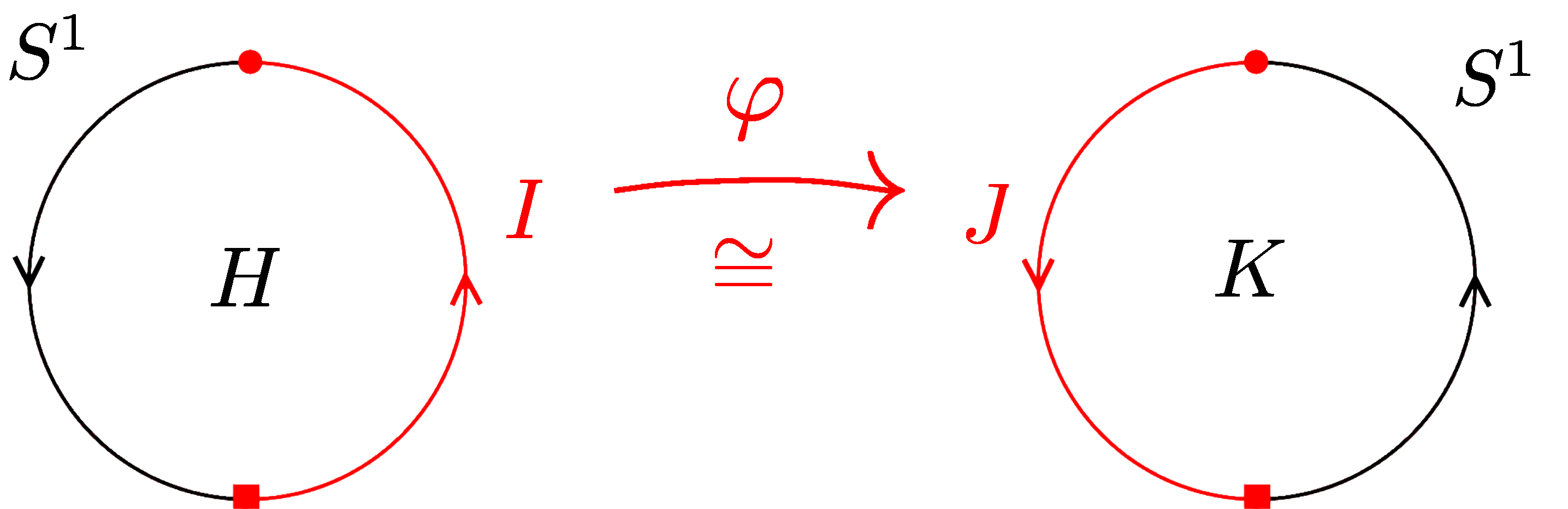
Figure 13. The diffeomorphism used to define the fusion product $H\boxtimes_{\mathcal{A}(J)}K$ between two representations $H$ and $K$ of a conformal net. One can think of $H$ as having actions of all the algebras corresponding to submanifolds of the circle enclosing it, and of $K$ as having actions of algebras living on the other circle.

In Section 4.2.1 we will describe a coordinate-independent approach to the representation theory of conformal nets, and to the fusion product of representations.

3.2.2. The loop group of $SU(2)$

To get a feeling of what representations of conformal nets are for the case of loop groups, we consider the simplest non-trivial case: the loop group $L\,SU(2)$ of $SU(2)$. Recall that $SU(2)$ has one irreducible representation $V_{n}$ of dimension $n+1$ for each $n\in\mathbb{N}$. $V_{0}$ is the trivial representation, $V_{1}$ is the fundamental representation, and so on. For $m\leq n$ the tensor product of two irreducible representations is given by the Clebsch-Gordan decomposition

(7) $$V_{m}\otimes V_{n}\cong V_{n-m}\oplus V_{n-m+2}\oplus\cdots\oplus V_{n+m}\ ,\qquad m\leq n\ .$$

This formula is already determined by the simpler relation

$$V_{1}\otimes V_{n}\cong V_{n-1}\oplus V_{n+1}\ ,\qquad n\geq 1\ .$$

Likewise, the representation theory of the loop group $L\,SU(2)_{k}$ of $SU(2)$ at level $k$ has irreducible representation $V_{0},\cdots\mspace{-1.0mu},V_{k}$, where now each of the $V_{n}$ is an infinite-dimensional Hilbert space. As before, $V_{0}$ is the monoidal unit and the fusion rules are entirely determined by the action of $V_{1}\boxtimes-$:

(8) $$V_{1}\boxtimes V_{n}\cong\begin{cases}V_{1}&\text{if }n=0\ ;\\ V_{n-1}\oplus V_{n+1}&\text{if }1\leq n\leq k-1\ ;\\ V_{k-1}&\text{if }n=k\ .\end{cases}$$

It is a nice exercise to use the above formulas to find the analogue of (7) for $L\,SU(2)_{k}$.

We repeat that the current state of knowledge about general loop group nets is somewhat incomplete, even though it is quite clear what should be the case. The cases $G=SU(n)$ is the only one where everything is known.

3.3. Conformal nets revisited

It is convenient to change the source category of conformal nets a bit: henceforth we restrict ourselves to contractible compact one-manifolds, i.e., to intervals. The circles can be recovered by gluing two intervals together.

Definition 1.

A conformal net $\mathcal{A}$ is a continuous functor from the category

$$\begin{cases}\ \text{objects: contractible compact oriented one-manifolds;}\\ \ \text{morphisms: embeddings}\end{cases}$$

to the category

$$\begin{cases}\ \text{objects: von Neumann algebras;}\\ \ \text{morphisms: injective homomorphisms and antihomomorphisms.}\end{cases}$$

An embedding $I\hookrightarrow J$ is sent to a homomorphism $\mathcal{A}(I)\hookrightarrow\mathcal{A}(J)$ if it preserves the orientation, and to a homomorphism $\mathcal{A}(I)\hookrightarrow\mathcal{A}(J)^{\text{op}}$ if it reverses the orientation. The hom-sets of the source category carry the $C^{\infty}$ topology, and there is also a topology on the hom-sets of the target category. It is with respect to these topologies that $\mathcal{A}$, mapping $I\hookrightarrow J$ to an (anti)homomorphism, has to be continuous. Moreover, a conformal net $\mathcal{A}$ is subject to the following axioms:

1. The algebras $\mathcal{A}\big{(}[0,1]\big{)}$ and $\mathcal{A}\big{(}[1,2]\big{)}$ commute in, and generate a dense subalgebra of $\mathcal{A}\big{(}[0,2]\big{)}$;

2. Denoting the algebraic tensor product by $\otimes_{\text{alg}}$ and the so-called spatial tensor product of von Neumann algebras by $\bar{\otimes}$, there exists an extension that makes the diagram commute:

3. The image of the map

   $$\big{\{}\ \varphi\in\text{Diff}\big{(}[0,3]\big{)}\ \ \colon\ \varphi|_{[0,1]}=\text{id}\,,\ \varphi|_{[2,3]}=\text{id}\ \big{\}}\longrightarrow\text{Aut}\big{(}\mathcal{A}([0,3])\big{)}$$

   is contained in the set of inner automorphisms of $\mathcal{A}([0,3])$;

4. There exists a dotted map such that the diagram

   commutes.

We pause to explain why $\text{Rep}\,(\mathcal{A})$ is braided. Let $I$ and $J$ be two halves of the standard circle, as in Figure 13. Given $H,K\in\text{Rep}\,(\mathcal{A})$, we need to construct the braiding isomorphism $H\boxtimes_{\mathcal{A}(J)}K\to K\boxtimes_{\mathcal{A}(J)}H$ in two steps. It is the composite of two ‘quarter-braiding’ isomorphisms

$$H\boxtimes_{\mathcal{A}(J)}K\,\longrightarrow\,H\boxtimes_{\mathcal{A}(J_{1})}K\,\longrightarrow\,H\boxtimes_{\mathcal{A}(I)}K\cong K\boxtimes_{\mathcal{A}(J)}H$$

where $I_{1}$ and $J_{1}$ form another decomposition of $S^{1}$ into half-circles (for example top and bottom halves). We focus on the first isomorphism, between $H\boxtimes_{\mathcal{A}(J)}K$ and $H\boxtimes_{\mathcal{A}(J_{1})}K$. Let $\varphi$ be a diffeomorphism of the circle that sends $I$ to $I_{1}$ and whose support does not cover the whole of $S^{1}$. Similarly, let $\psi$ be a diffeomorphism of the circle that sends $J$ to $J_{1}$ and whose support does not cover the whole of $S^{1}$. By axiom (iii) of the definition of conformal nets, there exist unitaries $u$ and $v$ such that $\text{Ad}(u)=\mathcal{A}(\varphi)$ and $\text{Ad}(v)=\mathcal{A}(\psi)$. Multiplication by $u$ on $H$ and by $v$ on $K$ induce a map $H\boxtimes_{\mathcal{A}(J)}K\to H\boxtimes_{\mathcal{A}(J_{1})}K$. Unfortunately this map does not have the right equivariance properties to be a morphism in $\text{Rep}\,(\mathcal{A})$. To fix that, we consider the diffeomorphism $\varphi|_{J}\cup\psi|_{I}$. Once again, its support is not the whole circle, and so by axiom (iii) we can find a unitary operator $w$ that corresponds to it, in one of the algebras that act on $H\boxtimes_{\mathcal{A}(J_{1})}K$. The quarter-braiding isomorphism is the composite

$$H\boxtimes_{\mathcal{A}(J)}K\,\xrightarrow{\,u\boxtimes v\,}\,H\boxtimes_{\mathcal{A}(J_{1})}K\,\stackrel{{\scriptstyle w^{*}}}{{\longrightarrow}}\,H\boxtimes_{\mathcal{A}(J_{1})}K.$$

There is a subtle point that we should mention: conformal nets have two roles in life. Although the relation with Segal’s definition of $\chi$cft may not be clear from the above definition, conformal nets, or rather, a subset of them, serve as a model for $\chi$cft (we should emphasize that, as far as the math is concerned, the relationship between conformal nets and other models of $\chi$cft is completely conjectural). On the other hand, conformal nets serve as a model for three-dimensional tqft, such as Chern-Simons theory. The conformal nets described in Definition 1 correspond to 3d tqfts. In order to have an associated $\chi$cfts, a conformal net needs to satisfy a further ‘positive energy’ condition. The latter says that, under the map in axiom (iii), the flow of a positive vector field in $\text{Diff}([0,3])$ correspond to a one-parameter group of unitaries in $\mathcal{A}([0,3])$ with positive generator (this generator is only well defined up to an additive constant). The loop group conformal nets satisfy both conditions and so they correspond to both a three-dimensional tqft and a two-dimensional $\chi$cft.

We should point out that, at least conjecturally, the $\chi$cft associated to a conformal net $\mathcal{A}$ (satisfying the positive energy condition) maps the circle to the representation category $\text{Rep}\,(\mathcal{A})$, so that the Frobenius algebra objects that occur in Section 3.5 and in Section 4 live in the same world. Also, we will not need the positive energy condition for the construction of the zero- and one-dimensional parts of the extended cft. That condition only gets used when constructing the operator associated to a bigon (such as the one in Figure 8).

3.4. Frobenius algebra objects

In Section 3.1 we have seen that a $\chi$cft assigns to the standard circle a category $\mathcal{C}$, and that the pair of pants equips that category with a monoidal structure. In our example of interest, this is the category

$$\mathcal{C}\coloneqq\text{Rep}\,(\mathcal{A}_{LG,k})\,\stackrel{{\scriptstyle\scriptscriptstyle(?)}}{{\cong}}\,\text{Rep}\,(L\,G_{k})$$

of representations of the conformal net $\mathcal{A}_{LG,k}$ associated to the loop group of $G$ at level $k$. This category is expected to be equivalent to the category of positive energy representations of $L\,G$ at level $k$. We are interested in objects of $\mathcal{C}$ with a particular kind of extra structure, which can be defined in any monoidal dagger category (a dagger category is a category $\mathcal{C}$ equipped with involutive antilinear maps $\dagger\!:\text{Hom}(X,Y)\to\text{Hom}(Y,X)$, $X,Y\in\mathcal{C}$ that assemble to a functor $\dagger:\mathcal{C}\to\mathcal{C}^{\mathrm{op}}$). Indeed, our category $\mathcal{C}$ consists of Hilbert spaces, so there is a notion of adjoints that turns it into a monoidal dagger category. Here, as before, the monoidal structure is given by the fusion product.

Definition.

A special symmetric Frobenius algebra object (we will simply call them Frobenius algebra objects) is an object $Q\in\mathcal{C}$ together with maps

• multiplication $m\colon Q\boxtimes Q\longrightarrow Q$ ,

• unit $m:1\longrightarrow Q$ , (here $1$ stands for the unit object of $\mathcal{C}$)

• comultiplication $\Delta\colon Q\longrightarrow Q\boxtimes Q$ , and

• counit $\varepsilon\colon Q\longrightarrow 1$ ,

subject to the axioms shown in Figure 15.

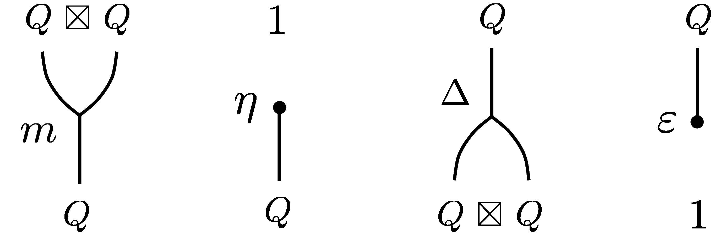
Figure 14. The building blocks of the string diagrams used in the definition (see Figure  15) of a Frobenius algebra object: (co)multiplication and (co)unit. The diagrams are read from top to bottom. The precise shape of the strings is not important. Because of the distinctive shapes the labels are usually omitted.

i)  

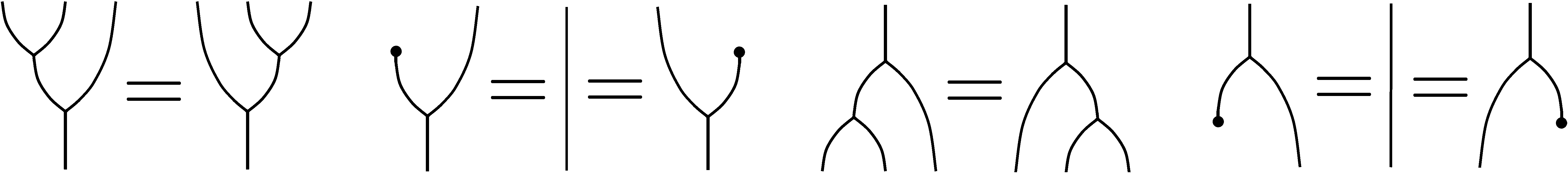
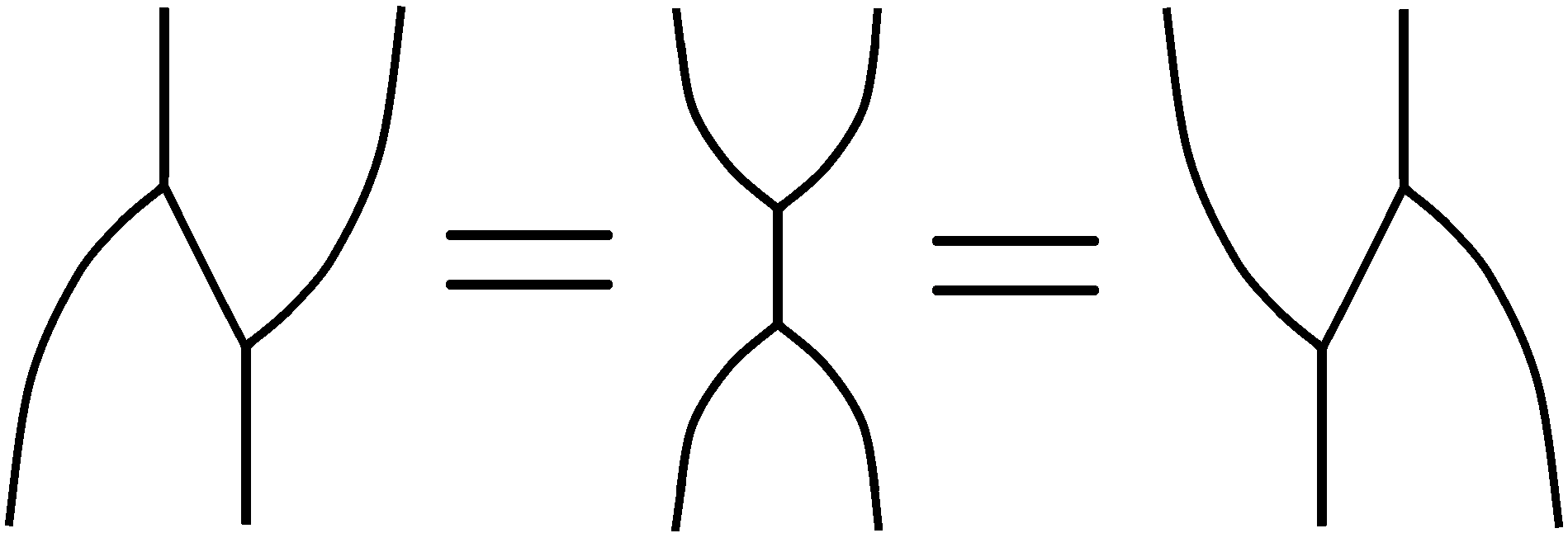
ii)       iii)  

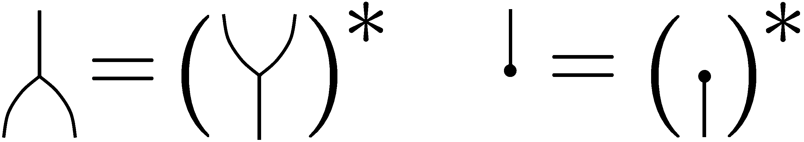
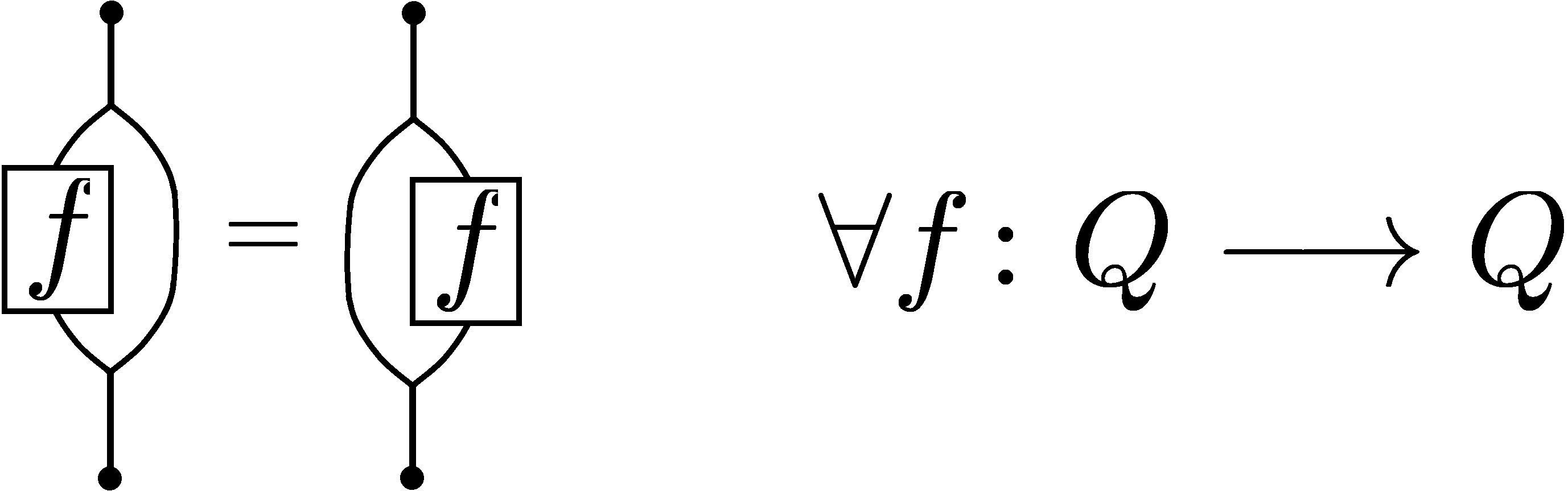
iv)             v)   

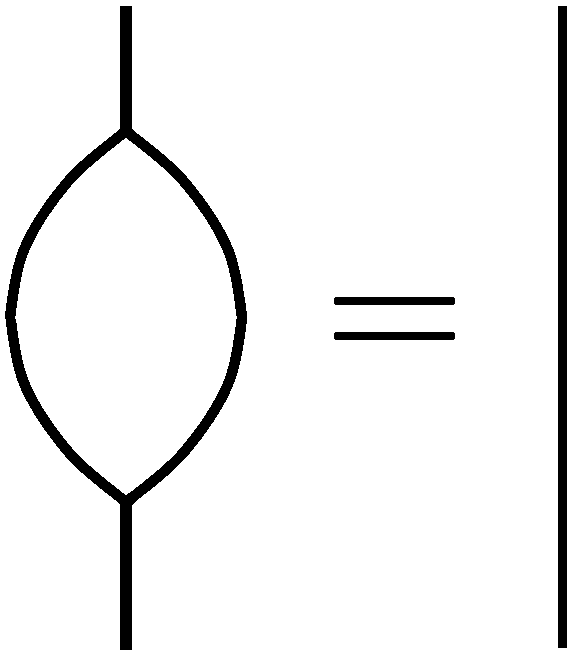
Figure 15. The axioms for a Frobenius algebra object.

Axiom (i) simply states that multiplication and comultiplication are associative and unital. Axiom (ii) is called the Frobenius condition. The third axiom implies that the coalgebra structure on $Q$ is determined by its algebra structure, by taking adjoints.

Axiom (iv) requires $Q$ to be symmetric, and is equivalent to the condition $\vbox{\hbox{ \leavevmode\hbox to19.01pt{\vbox to19.92pt{\text{[drawing]}}}}}=\vbox{\hbox{ \leavevmode\hbox to19.01pt{\vbox to19.92pt{\text{[drawing]}}}}}$ from [FRS02].

Finally, axiom (v) is called the special property. The special property means that a Frobenius algebra object is very different from e.g. cohomology rings of manifolds. In particular, it implies that the algebra $Q$ is semisimple: any module over $Q$ is semisimple.

The definition of a Frobenius algebra object may look complicated, but a Frobenius algebra is just an algebra satisfying certain properties: everything is determined by the multiplication and unit maps.

3.4.1. Examples

To get a feeling for what Frobenius algebras can look like, let us have a look at some examples. Since every semisimple algebra is a direct sum of simple algebras, we restrict our attention to simple algebras.

A trivial example of a Frobenius algebra object is the unit object of the monoidal category.

For another example, consider an object $X\in\mathcal{C}$ and form the Connes fusion $Q=X\boxtimes X^{\vee}$ of the object with its dual. Then $Q$ is an algebra, indeed a Frobenius algebra. This is the correct generalization of matrix algebras to this context. For instance, taking $\mathcal{C}=\text{Rep}\big{(}LSU(2)_{2}\big{)}$ and $X=V_{1}$, then $X^{\vee}\cong V_{1}$ too and (8) yields $Q=V_{0}\oplus V_{2}$. But $X\boxtimes X^{\vee}$ is Morita equivalent to the unit object (see Section 3.5.3), so this is still not a very interesting example. However, it leads us to the next example.

Let $\mathcal{C}_{k}=\text{Rep}\big{(}LSU(2)_{k}\big{)}$ for arbitrary $k$. In $\mathcal{C}_{k}$, we have

(9) $$V_{0}\boxtimes V_{0}\cong V_{0}\ ,\quad V_{0}\boxtimes V_{k}\cong V_{k}\ ,\quad V_{k}\boxtimes V_{0}\cong V_{k}\ ,\quad V_{k}\boxtimes V_{k}\cong V_{0}\ .$$

These relations show that the full subcategory of $\mathcal{C}_{k}$ consisting of objects isomorphic to sums of $V_{0}$ and $V_{k}$ is again a monoidal category. The monoidal structure is not fully determined by the relations 9; rather, up to equivalence of monoidal categories, there are two different monoidal categories that satisfy 9. One is the category of $\mathbb{Z}_{/2}$-graded vector spaces, and the other is a version of it where the associator is twisted by a cocycle $c$ representing a non-trivial cohomology class $[c]\in H^{3}(\mathbb{Z}_{/2},S^{1})\cong\mathbb{Z}_{/2}$. It turns out that the subcategory of $\mathcal{C}_{k}$ is equivalent to the category of $\mathbb{Z}_{/2}$-graded vector spaces only if $k$ is even, and $Q=V_{0}\oplus V_{k}$ has a Frobenius algebra structure if and only if $[c]=0$, if and only if $k$ is even.

3.4.2. Classification

There is a beautiful classification of all simple Frobenius algebra objects in $\mathcal{C}_{k}=\text{Rep}\big{(}LSU(2)_{k}\big{)}$ due to Ostrik [Ost03] (inspired by the CIZ classification of modular invariants for $\hat{\mathfrak{sl}}(2)$ cfts [CIZ87]) that goes as follows.

Up to Morita equivalence, Frobenius algebra objects in $\mathcal{C}_{k}$ fall in two infinite families corresponding to the following Dynkin diagrams:

$$\text{type $A_{n}$:}\qquad Q=V_{0}\ ,\quad k=n-1\ ,\quad\quad(n\geq 1)$$

$$\text{type $D_{n}$:}\qquad Q=V_{0}\oplus V_{k}\ ,\quad k=2n-4\ ,\quad\quad(n\geq 4).$$

In addition, there are three exceptional cases:

$$\text{type $E_{6}$:}\qquad Q=V_{0}\oplus V_{6}\ ,\quad k=10\ ,$$

$$\text{type $E_{7}$:}\qquad Q=V_{0}\oplus V_{8}\oplus V_{16}\ ,\quad k=16\ ,$$

$$\text{type $E_{8}$:}\qquad Q=V_{0}\oplus V_{10}\oplus V_{18}\oplus V_{28}\ ,\quad k=28\ .$$

For each type we have listed a representative $Q$ of the Morita equivalence class.

3.5. The FRS construction

In Section 3.2.1 we have mentioned that there is a construction that takes a chiral cft as input, along with a Frobenius algebra object in the category $\mathcal{C}$ provided by the $\chi$cft, and produces a full cft as output.

In the realm of algebraic quantum field theory, this result is due to Longo and Rehren [LR04, KL04b]. They start with a conformal net and a Frobenius algebra object, and construct a net of von Neumann algebras on $\mathbb{R}^{2}$ with its Minkowski signature. Such a net assign von Neumann algebras to open subsets of $\mathbb{R}^{2}$ in such a way that the algebras commute if the opens are causally separated.

Instead of elaborating on this construction we will discuss another approach, which is due to Fuchs, Runkel and Schweigert [FRS02, FRS04a, FRS04b, FRS05, FRS06]. This is a big body of work, and we will only outline some of its aspects.

3.5.1. The partition function

Let us at least describe how to take a $\chi$cft and a Frobenius algebra object and assign a number $Z(\Sigma)\in\mathbb{C}$ to a closed Riemann surface $\Sigma$ (c.f. the discussion in Section 2.1).

A $\chi$cft assigns to $\Sigma$ a functor $\mathcal{C}_{\text{in}}\longrightarrow\mathcal{C}_{\text{out}}$. Recall that a non-extended $\chi$cft assigns to a closed surface $\Sigma$ a linear map $\mathbb{C}\longrightarrow\mathbb{C}$, which is completely determined by an element of $\mathbb{C}$. In the present context, something similar happens. The category $\mathsf{Vect}$ is the unit object of the target category $\mathsf{LinCat}$ of $\mathbb{C}$-linear categories. Indeed, $\mathsf{LinCat}$ is equipped with a tensor product operation, say $\otimes$, such that, for any linear category $\mathcal{C}$, $\mathsf{Vect}\otimes\mathcal{C}=\mathcal{C}$. Now a linear functor $f\colon\mathsf{Vect}\longrightarrow\mathsf{Vect}$ is completely determined by the image $V\coloneqq f(\mathbb{C})$, so for any $X\in\mathsf{Vect}$ we have $f(X)=X\otimes V$. The vector space $V$ associated to the functor $\mathcal{C}_{\text{in}}\longrightarrow\mathcal{C}_{\text{out}}$ is called the space of conformal blocks associated to $\Sigma$ by the $\chi$cft. There is also a canonical element $\omega\in V$ provided by the structure of the $\chi$cft: it is the image

$$\mathbb{C}=H_{\lambda}\longrightarrow H_{f(\lambda)}=V\ ,\quad 1\longmapsto\ \omega\ ,$$

for $\lambda=\mathbb{C}\in\mathsf{Vect}=\mathcal{C}_{\text{in}}$.

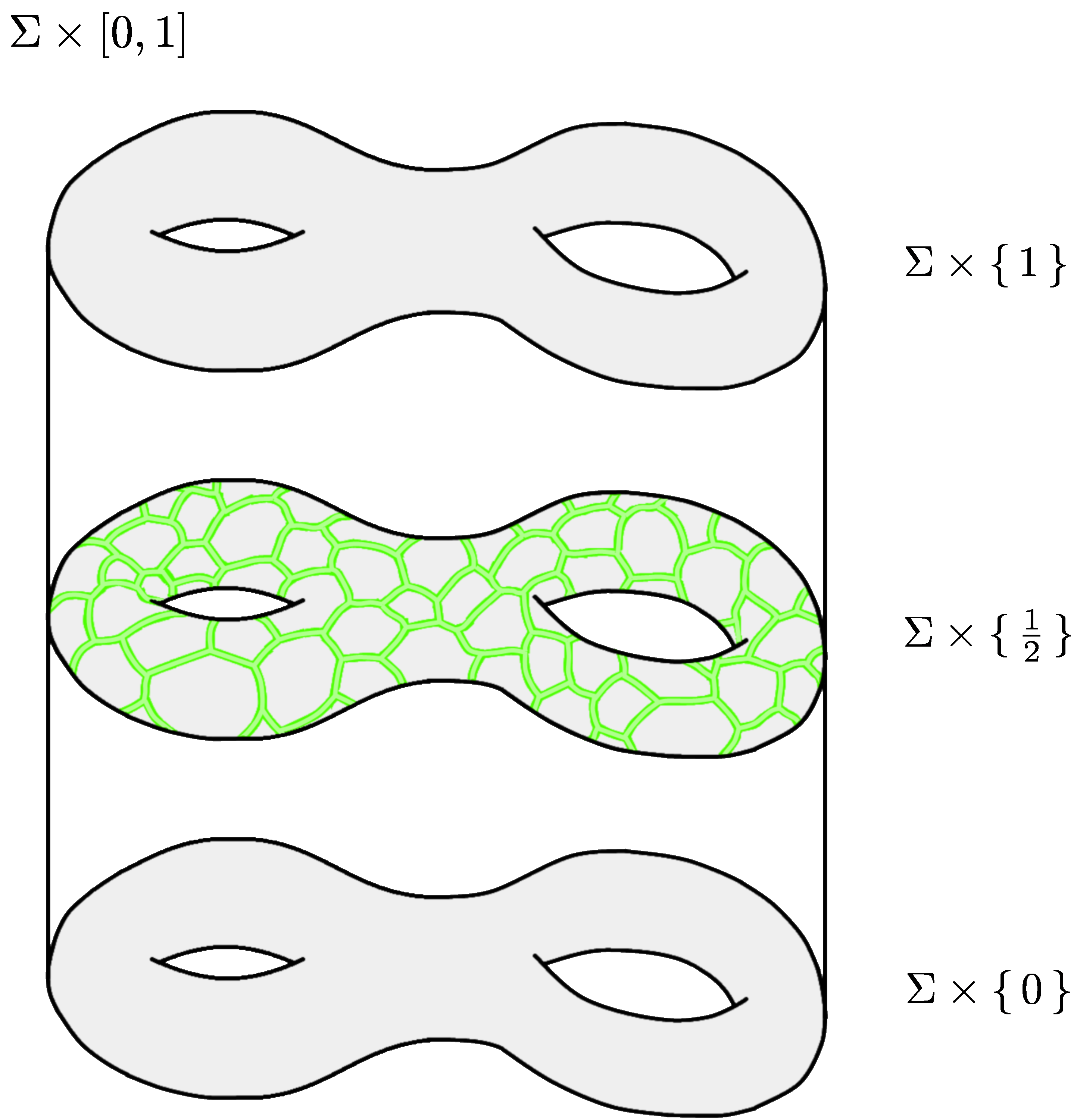
Figure 16. The product of a closed Riemann surface $\Sigma$ with the unit interval. The middle slice is decorated by a ribbon graph with trivalent vertices. Actually, the middle slice $\Sigma\times\{\frac{1}{2}\}$ should not be there in the picture; it is only needed to explain where the ribbon graph sits.

To see where the Frobenius algebra object comes in, consider the 3-manifold $\Sigma\times[0,1]$ which is obtained by crossing $\Sigma$ with a unit interval. Decorate the middle slice $\Sigma\times\{\frac{1}{2}\}$ with a ribbon graph, whose edges are ‘thickened’ to little two-dimensional ribbons, as shown in Figure 16. We only allow for trivalent vertices. Now give the ribbons an orientation, so as to get a directed ribbon graph. This can always be done in such a way that each vertex has at least one incoming ribbon and at least one outgoing ribbon. This allows us to further color the graph with the Frobenius algebra object $Q$ and its multiplication $m$ and comultiplication $\Delta$ according to the rules shown in Figure 17.

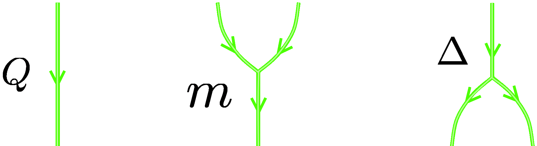
Figure 17. A directed ribbon graph with trivalent vertices can always be colored by these rules (cf. the string diagrams for the (co)multiplication of Frobenius algebra objects in Figure 14).

In order to assign a number to $\Sigma$, FRS invoke the existence of a three-dimensional topological quantum field theory (tqft). The latter assigns to the three-manifold $\Sigma\times[0,1]$ with colored ribbon graph an element $c\in V\otimes\bar{V}$ of the conformal blocks of $\partial\big{(}\Sigma\times[0,1]\big{)}=\Sigma\sqcup\bar{\Sigma}$. Here, $\bar{\Sigma}$ denotes the manifold $\Sigma$ with the reversed orientation. The partition function is then given by

$$Z(\Sigma)=\langle\,c\,,\,\omega\otimes\bar{\omega}\,\rangle_{V\otimes\bar{V}}\in\mathbb{C}\ .$$

Using the axioms of a (special symmetric) Frobenius algebra object, one can then show that this number does depend neither on the choice of ribbon graph nor on the orientation of the ribbons.

3.5.2. The state space

The next question concerns the state space of the cft: what is the Hilbert space associated to a circle? For that, one considers the same kind of picture as above, but with a hole, as shown in Figure 18.

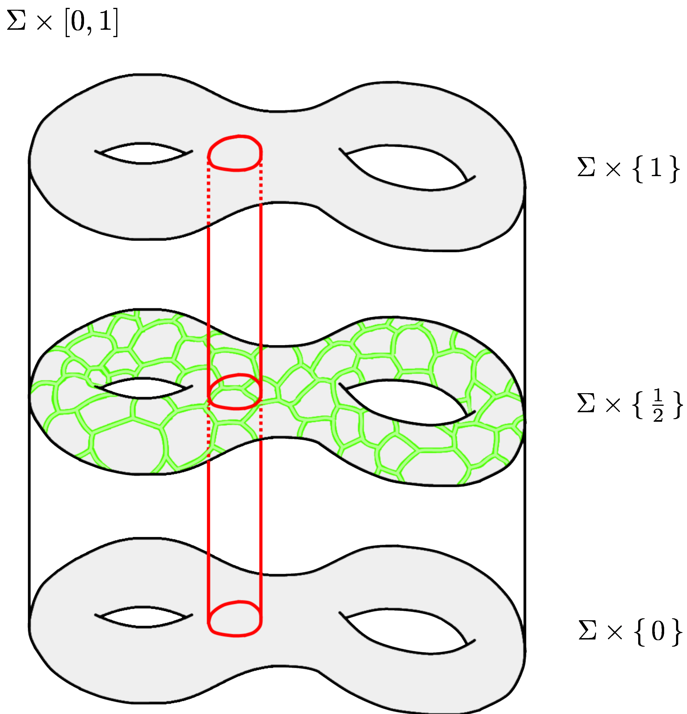
Figure 18. The product of a closed Riemann surface $\Sigma$ with the unit interval, with a cylinder taken out.

We would like to add a single ribbon going down the middle of the hole, in such a way that it is compatible with the ribbon graph on the surface $\Sigma\times\{\frac{1}{2}\}$. Imagine a single strand coming from above, along with another one coming from below. The question is: what do we label these by? Since there are two strands (one from above, and one from below), we are looking for two objects of $\mathcal{C}$. More accurately, we are looking for one object in $\mathcal{C}$ and one in $\bar{\mathcal{C}}$, where the bar now stands for complex conjugation (the category $\bar{\mathcal{C}}$ has the same objects as $\mathcal{C}$, but $\text{Hom}_{\bar{\mathcal{C}}}(\lambda,\mu)$ is the complex conjugate of $\text{Hom}_{\mathcal{C}}(\lambda,\mu)$. Given an object $\lambda\in\mathcal{C}$, we shall denote by $\bar{\lambda}$ the corresponding object of $\bar{\mathcal{C}}$. The Hilbert space $H_{\bar{\lambda}}$ associated to $\bar{\lambda}\in\bar{\mathcal{C}}$ is then the complex conjugate of the Hilbert space $H_{\lambda}$ associated to $\lambda\in\mathcal{C}$). Equivalently, we are looking for a single object of $\mathcal{C}\times\bar{\mathcal{C}}$. It turns out that this is not quite general enough. What we are really after is an object of $\mathcal{C}\otimes\bar{\mathcal{C}}$, that is, a formal direct sum of objects of $\mathcal{C}\times\bar{\mathcal{C}}$.

To see what the compatibility condition is, consider a juncture of the ribbon in the cylinder with a ribbon from $\Sigma\times\{\frac{1}{2}\}$, as depicted in Figure 19. The ribbon graph can always be arranged so that there is such a junction.

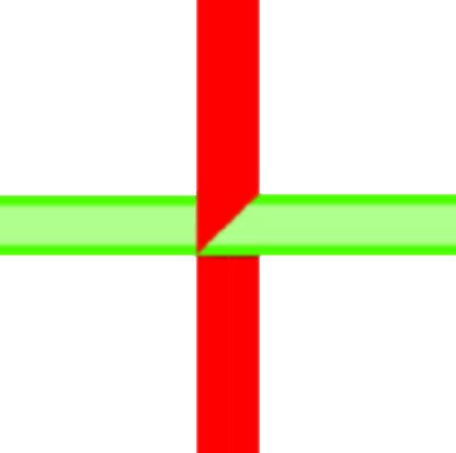
Figure 19. A junction between the ribbon that is dangling down in the cylinder and a ribbon from the graph on $\Sigma\times\{\,\frac{1}{2}\,\}$.

The value (object of $\mathcal{C}\otimes\bar{\mathcal{C}}$) that is assigned to the ribbon on the cylinder has to satisfy the compatibility requirements shown in Figure 20.

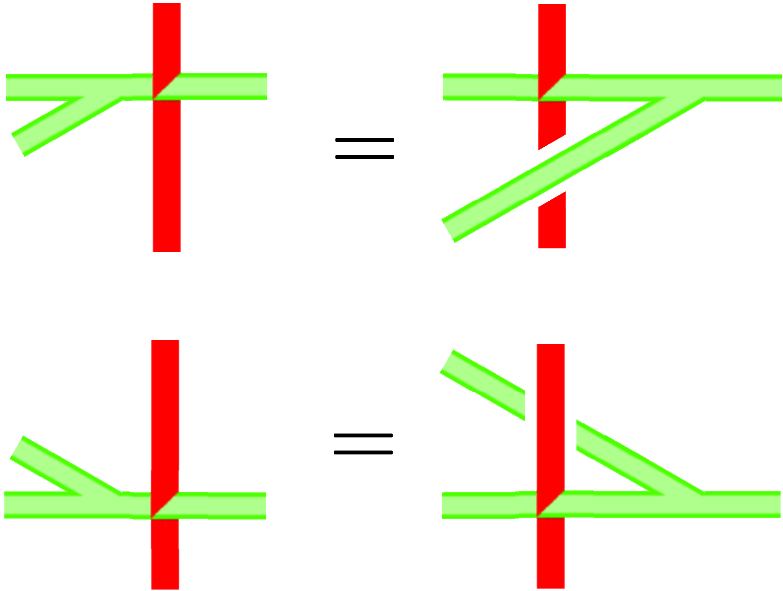
Figure 20. Compatibility requirements between the vertical ribbon in the cylinder (cf. Figure 18) and the ribbons of the graph on $\Sigma\times\{\,\frac{1}{2}\,\}$.

It turns out that there is an object that is universal with respect to these properties: the full centre of $Q$, given by

(10) $$Z_{\text{full}}(Q)=\bigoplus_{\mu,\lambda}\text{Hom}_{Q,Q}\big{(}\lambda\boxtimes^{+}Q\boxtimes^{-}\mu^{\vee},Q\big{)}\otimes\lambda\otimes\bar{\mu}\ \in\mathcal{C}\otimes\bar{\mathcal{C}}\ .$$

This equation require some explanations. First of all, $\mu^{\vee}$ is the dual of $\mu$, characterized by the existence of a non-zero map $1\to\mu\boxtimes\mu^{\vee}$. The symbols $\boxtimes^{\pm}$ denote the tensor product from above and below (as opposed to from right or from the left), which can be defined because the monoidal category $\mathcal{C}$ is braided. So $\lambda\boxtimes^{+}Q\boxtimes^{-}\mu^{\vee}$ could more accurately be drawn as .
That object is a $Q$-$Q$-bimodule: it comes with maps $Q\boxtimes(\lambda\boxtimes^{+}Q\boxtimes^{-}\mu^{\vee})\to\lambda\boxtimes^{+}Q\boxtimes^{-}\mu^{\vee}$ and $(\lambda\boxtimes^{+}Q\boxtimes^{-}\mu^{\vee})\boxtimes Q\to\lambda\boxtimes^{+}Q\boxtimes^{-}\mu^{\vee}$ induced from the left and right actions of $Q$ on itself. (The reader who finds $\boxtimes^{\pm}$ unpleasant can take $\lambda\boxtimes^{+}Q\boxtimes^{-}\mu^{\vee}$ to simply mean $\lambda\boxtimes Q\boxtimes\mu^{\vee}$; the braiding is then used to endow this object with the structure of a $Q$-$Q$-bimodule.) Finally, $\text{Hom}_{Q,Q}$ in (10) refers to the space of bimodule homomorphisms. Since this is a vector space, while $\lambda\in\mathcal{C}$ and $\bar{\mu}\in\bar{\mathcal{C}}$, the full centre of $Q$ is an object of $\mathcal{C}\otimes\bar{\mathcal{C}}$.

The state space of the full cft associated to the $\chi$cft together with the Frobenius algebra object $Q$ is then given by

(11) $$H_{\text{full}}\coloneqq\bigoplus_{\mu,\lambda}\text{Hom}_{Q,Q}\big{(}\lambda\boxtimes^{+}Q\boxtimes^{-}\mu^{\vee},Q\big{)}\otimes H_{\lambda}\otimes\overline{H_{\mu}}\ .$$

In the ‘Cardy case’, where $Q=1$ is the unit object, this expression reduces to $H_{\text{full}}=\bigoplus_{\lambda}H_{\lambda}\otimes\overline{H_{\lambda}}$.

Equation (11) is the result of FRS that we were after. The discussion in Section 3.5 mainly serves to provide some motivation for this result, as it is very important for the remainder. Indeed, below we will reproduce this result in the context of extended cft. We will define what an extended cft assigns to points and to intervals. Then we will take the two halves of a circle, and fuse them over the algebra associated to their boundary. Comparing the resulting Hilbert space with (11) will provide a check of our formalism.

3.5.3. Defects

We mention one more feature of the FRS construction. Recall that two algebras $A$ and $B$ are said to be Morita equivalent if there exist bimodules ${}_{A}X_{B}$ and ${}_{B}Y_{A}$ such that there are isomorphisms

$${}_{A}X\otimes_{B}Y_{A}\cong{}_{A}A_{A}\quad\text{and}\quad{}_{B}Y\otimes_{A}X_{B}\cong{}_{B}B_{B}\ .$$

Now if we have two Frobenius algebra objects $Q$ and $Q^{\prime}$ that are Morita equivalent (with the definition interpreted internally to the category $\mathcal{C}$), the resulting full cft does not change. In particular, we get the same state space (11).

Kapustin and Saulina [KS11] have a nice way of reinterpreting this fact. Recall the special property, axiom (v) from Section 3.4, of our Frobenius algebra. Figure 21 shows the special property in terms of the directed ribbon graph on $\Sigma\times\{\frac{1}{2}\}$.

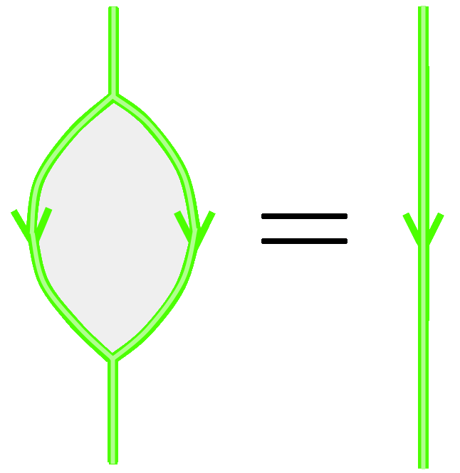
Figure 21. The special property of Frobenius algebra objects allows us to fill in the holes in a ribbon graph.

In other words: we can fill in the holes in the graph. If we do this everywhere, we get a three-manifold with an embedded surface, and the result looks like in Figure 22.

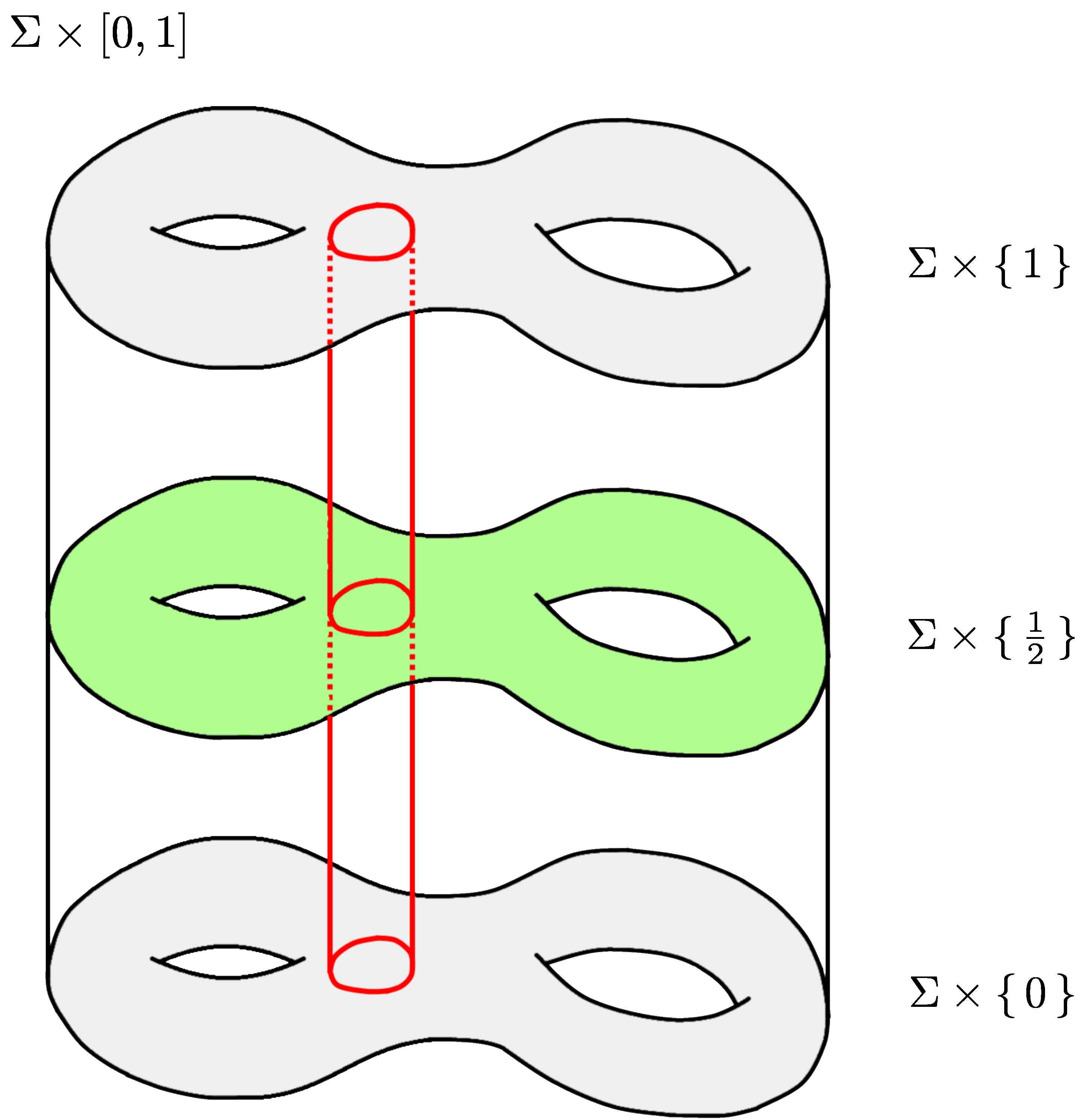
Figure 22. The product of a closed Riemann surface $\Sigma$ with the unit interval. The holes in the ribbon graph on $\Sigma\times\{\frac{1}{2}\}$ have been filled using the special property of the Frobenius algebra.

The three-manifold $\Sigma\times[0,1]$ now is decorated by a codimension-one defect (‘surface operator’). According to [KS11] this defect only contains the information of the Morita equivalence class of $Q$, and not of $Q$ itself. Moreover, one can go back to the ribbons and reinterpret them as actual embedded surfaces whose one-dimensional boundaries are labelled by $Q$ and whose two-dimensional interior corresponds to the defect. Upon filling in the holes in the ribbon graph we get rid of the boundary lines, we no longer see $Q$, but only its Morita equivalence class, in the form of a defect.

The partition function of $\Sigma$ is then obtained by evaluating the three-dimensional tqft on this three-manifold with defect.

3.5.4. Defects between conformal nets

The last ingredient we need in order to make sense of the three-manifold $\Sigma\times[0,1]$ with embedded surface within the formalism of conformal nets is the notion of a defect, leading to defects between conformal nets [BDH09]. For the purpose of the previous discussion, we would only need defects from a conformal net to itself. But in general, defects behave like bimodules: given two conformal nets $\mathcal{A}$ and $\mathcal{B}$, there is a notion of an $\mathcal{A}$-$\mathcal{B}$-defect ${}_{\mathcal{A}}D_{\mathcal{B}}$.

Definitions.

A bicolored interval is a contractible one-manifold $I$ equipped with a decomposition $I=I^{\prime}\cup I^{\prime\prime}$ that looks like one of

along with a local coordinate at the color-changing point.

A defect between conformal nets $\mathcal{A}$ and $\mathcal{B}$ is a functor from the category

$$\begin{cases}\ \text{objects: bicolored intervals;}\\ \ \text{morphisms: color preserving embeddings that respect the local coordinate;}\end{cases}$$

to the category

$$\begin{cases}\ \text{objects: von Neumann algebras;}\\ \ \text{morphisms: homomorphisms and antihomomorphisms;}\end{cases}$$

sending an embedding $I\hookrightarrow J$ to a homomorphism $D(I)\to D(J)$ if it preserves orientation, and to an antihomomorphism $D(I)\to D(J)^{\text{op}}$ if it reverses orientation. We have that $D(I)=\mathcal{A}(I)$ if $I^{\prime\prime}$ is empty, and $D(I)=\mathcal{B}(I)$ if $I^{\prime}$ is empty. Moreover, $D$ satisfies axioms similar to those of conformal nets.

4. Constructing extended conformal field theories

Until this point we have mostly discussed the work of others. It is time to come back to extended cft. In this section we will partially construct an extended cft starting from a $\chi$cft that is given to us in the form of a conformal net $\mathcal{A}$, and a Frobenius algebra object $Q\in\text{Rep}\,(\mathcal{A})$.

Recall from Section 3.2.1 that a representation of $\mathcal{A}$ consists of a Hilbert space $H$ equipped with compatible actions of $\mathcal{A}(I)$ for every $I\subsetneq S^{1}$. In Section 3.2.2 we have seen how the monoidal structure on $\text{Rep}\,(\mathcal{A})$ is defined: we identify the left half and the right half of $S^{1}$ with $[0,1]$ and set $A\coloneqq\mathcal{A}\big{(}[0,1]\big{)}$. This provides a fully faithful embedding of $\text{Rep}\,(\mathcal{A})$ into the category of $A$-$A$-bimodules, and the tensor product on $\text{Rep}\,(\mathcal{A})$ is inherited from the monoidal structure on $A$-$A$-bimodules:

$$(H,K)\longmapsto H\boxtimes_{A}K\,.$$

We can therefore view the Hilbert space $Q$ as an $A$-$A$-bimodule.

4.1. The algebra associated to a point

We start with dimension zero. The algebra that is associated to a point can be defined in the world of $A$-$A$-bimodules:

(12) $$B\coloneqq\text{Hom}\big{(}L^{2}A_{A},Q_{A}\big{)}$$

This is the set of bounded linear maps that commute with the right action of $A$. The algebra (12) also appears in the work of Longo and Rehren [LR04]; here we present a different construction of it. The reason that this works is the following surprising fact.

Lemma 4.1.

The vector space $B$ is an algebra, and indeed a von Neumann algebra. Moreover, there is an algebra homomorphism $A\longrightarrow B$.

Proof of Lemma 4.1..

Let us sketch the proof. For convenience we abbreviate $1\coloneqq L^{2}A$ and write $\boxtimes$ instead of $\boxtimes_{A}$. Recall that the Frobenius algebra object $Q$ comes equipped with a multiplication $m\colon Q\boxtimes Q\longrightarrow Q$, a unit $\eta\colon 1\longrightarrow A$ and comultiplication $\Delta=m^{*}$ and $\varepsilon=\eta^{*}$. We have to define a product, unit, and an involution on $B$, and show that it is a von Neumann algebra.

Let $f$ and $g$ be elements of $B$. The product of $f$ and $g$ is defined as the composition

$$f\cdot g\colon 1\xrightarrow{\ g\ }Q\cong 1\boxtimes Q\xrightarrow{\ f\times 1\ }Q\boxtimes Q\xrightarrow{\ m\ }Q\ .$$

Figure 23 shows how this rule can be represented graphically. Using the diagrams it is clear that the product is associative.

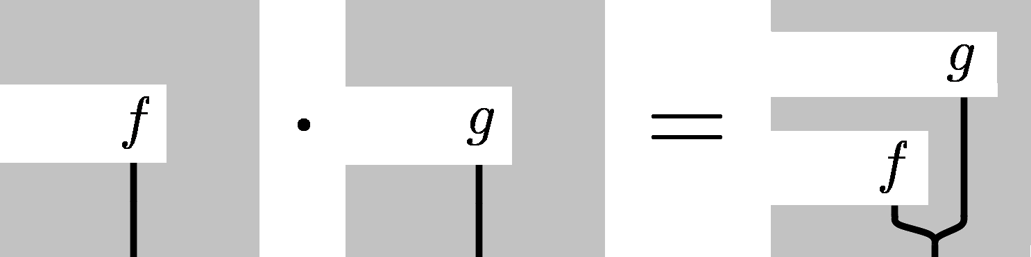
Figure 23. Diagrammatic representation of the product of $f,g\in B$. It should be understood as follows. Consider the diagram on the left, representing $f$. As with the string diagrams in Section 3.4 we start at the top, which is empty, corresponding to the unit. Then we apply $f$, which is only linear with respect to the right action of $A$, so that the left-hand side is ‘blocked’. In this way, the diagram exactly shows which operations are allowed algebraically. Finally, the line going to the bottom represents a copy of $Q$.

The unit of $B$ is just the unit map $\eta\colon 1\longrightarrow Q$ as shown in Figure 24. Together with the above product this determines the algebra structure on $B$.

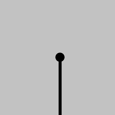
Figure 24. Diagrammatic representation of the unit map on $B$ is the same as in the string diagrams for Frobenius algebra objects (cf. Figure 14).

Next, the involution is denoted by ^⋆ and is defined as the following composition

$$f^{\star}\colon 1\xrightarrow{\ \eta\ }Q\xrightarrow{\ \Delta\ }Q\boxtimes Q\xrightarrow{\ f^{*}\times 1\ }1\boxtimes Q\cong Q\ .$$

See Figure 25 for the corresponding diagram.

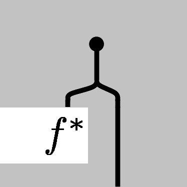
Figure 25. Diagrammatic representation of the involution of $f\in B$.

There is also a map from $A$ to $B$, sending an element $a\in A$ to the composition of left multiplication by $a$ with the unit:

$$a\colon 1\xrightarrow{\ a\cdot\ }1\xrightarrow{\ \eta\ }Q\ .$$

This can be represented as shown in Figure 26.

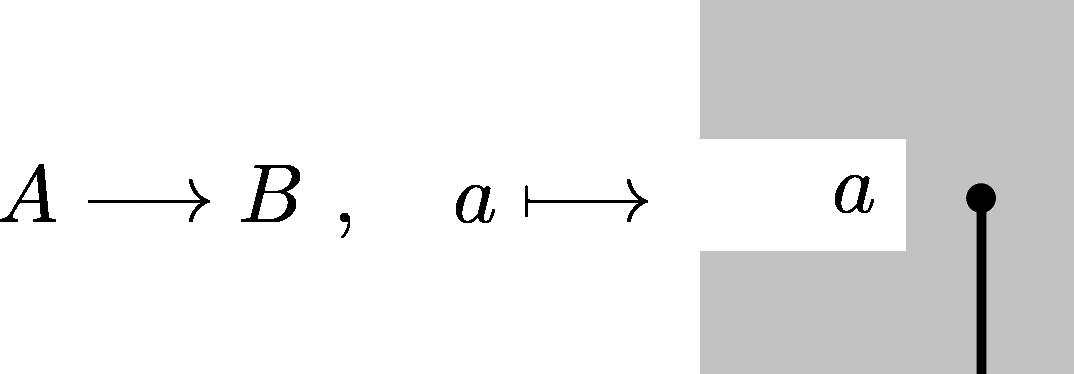
Figure 26. Diagrammatic representation of the map $A\longrightarrow B$.

Let $B(H)$ denote the set of bounded operators on the underlying Hilbert space $H$ of $Q$. The algebra $B$ acts on $H$ via

$$B \longrightarrow B(H)\ ,$$

$$f\mspace{1.0mu} \longmapsto\big{[}\ Q\cong 1\boxtimes Q\xrightarrow{\ f\times 1\ }Q\boxtimes Q\xrightarrow{\ m\ }Q\ \big{]}\ .$$

The image of $f\in B$ is shown in Figure 27.

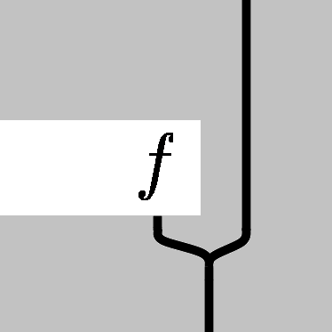
Figure 27. Diagrammatic representation of the left action of $B$ on the Frobenius algebra object $Q$.

Actually, $Q$ is a $B$-$B$-bimodule. The right $B$-action is shown in Figure 28. It uses the fact that $Q$ is its own dual (the pairing $\varepsilon\circ m$ is nondegenerate) and that for von Neumann bimodules there is a canonical identification between the dual and the complex conjugate. Therefore we can take the complex conjugate $\bar{f}$ of $f$ to get a left $A$-linear map.

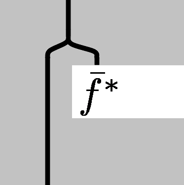
Figure 28. Diagrammatic representation of the left action of $B$ on the Frobenius algebra object $Q$.

Finally, one can show that the commutant of the left action of $B$ on $Q$ is the right action of $B$ on $Q$, and vice versa. The algebra $B$ is its own bicommutant, and therefore a von Neumann algebra. ∎

One can also check that the Hilbert space $Q$ is canonically isomorphic to $L^{2}B$ as a $B$-$B$-bimodule. In order to show that, one has to construct a positive cone $P\subset Q$ (which corresponds to $L_{+}^{2}B$), and define the modular conjugation $J:Q\longrightarrow Q$. Those should then satisfy the axioms listed in [Haa75]. The cone is defined as $P:=\{b\,\xi\,b^{*}\,|\,b\in B,\xi\in L^{2}_{+}A\}$. To construct the modular conjugation, one uses the identification ${}_{A}Q_{A}\cong{}_{A}Q^{\vee}_{A}$ coming from the pairing  , along with the fact that the dual of a bimodule is always its complex conjugate. We can then define $J$ to be the composite isomorphism $Q\,\cong\,Q^{\vee}\,\cong\,\overline{Q}$.

Recall that the zero-manifolds in the source bicategory of our three-tier cft are generated by two local models: a point with a sign. If $B_{+}$ is the von Neumann algebra (12) associated to the point with positive orientation, and $B_{-}$ the von Neumann algebra associated to the point with negative orientation, then $B_{+}$ is canonically isomorphic to $B_{-}^{\text{op}}$.

One can reinterpret the above construction as that of a defect from $\mathcal{A}$ to $\mathcal{A}$. Namely, there exists a defect $D$, constructed from the Frobenius algebra object $Q$, such that $D\big{(}[0,1]\big{)}=B$.

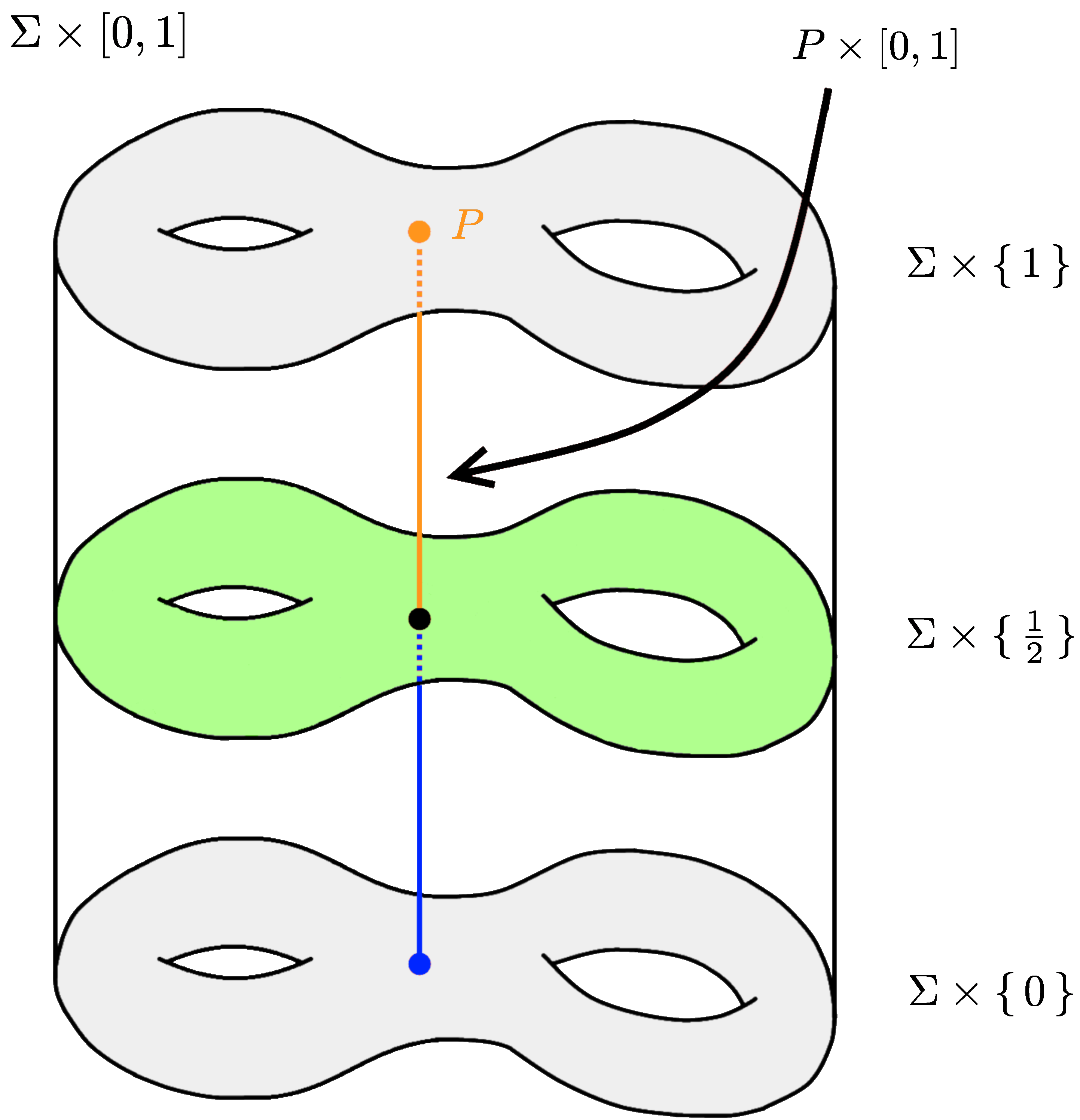
Figure 29. The construction of the algebra $B$ associated to a point $P\in\Sigma$ in the context of the FRS/Kapustin-Saulina construction.

Figure 29 shows the corresponding defect in the FRS construction. This is a rather special kind of defect, where the precise location in $[0,1]$ where the colors change is actually not important: the only thing that matters is that the interval $[0,1]$ is genuinely bicolored. Such defects are called topological defects. The defect that appeared in Section 3.5.3 is also a topological defect: what the tqft assigns to a manifold does not change at all when the location of the defect is moved a bit upwards or downwards.

4.2. The bimodule associated to an interval

Points do not have any geometry, and indeed the discussion above was very algebraic. Next we have to decide what to associate to an interval; this will involve some geometry.

We have already seen that, in order to evaluate our extended cft on a point $P$, we have to form the product $P\times[0,1]$, and evaluate our defect $D$ on the resulting one-manifold. In the present case we start with an interval $I$. We are again supposed to cross with $[0,1]$ and do something involving the defect, or, equivalently, with the Frobenius algebra object $Q$ — see Figure 30.

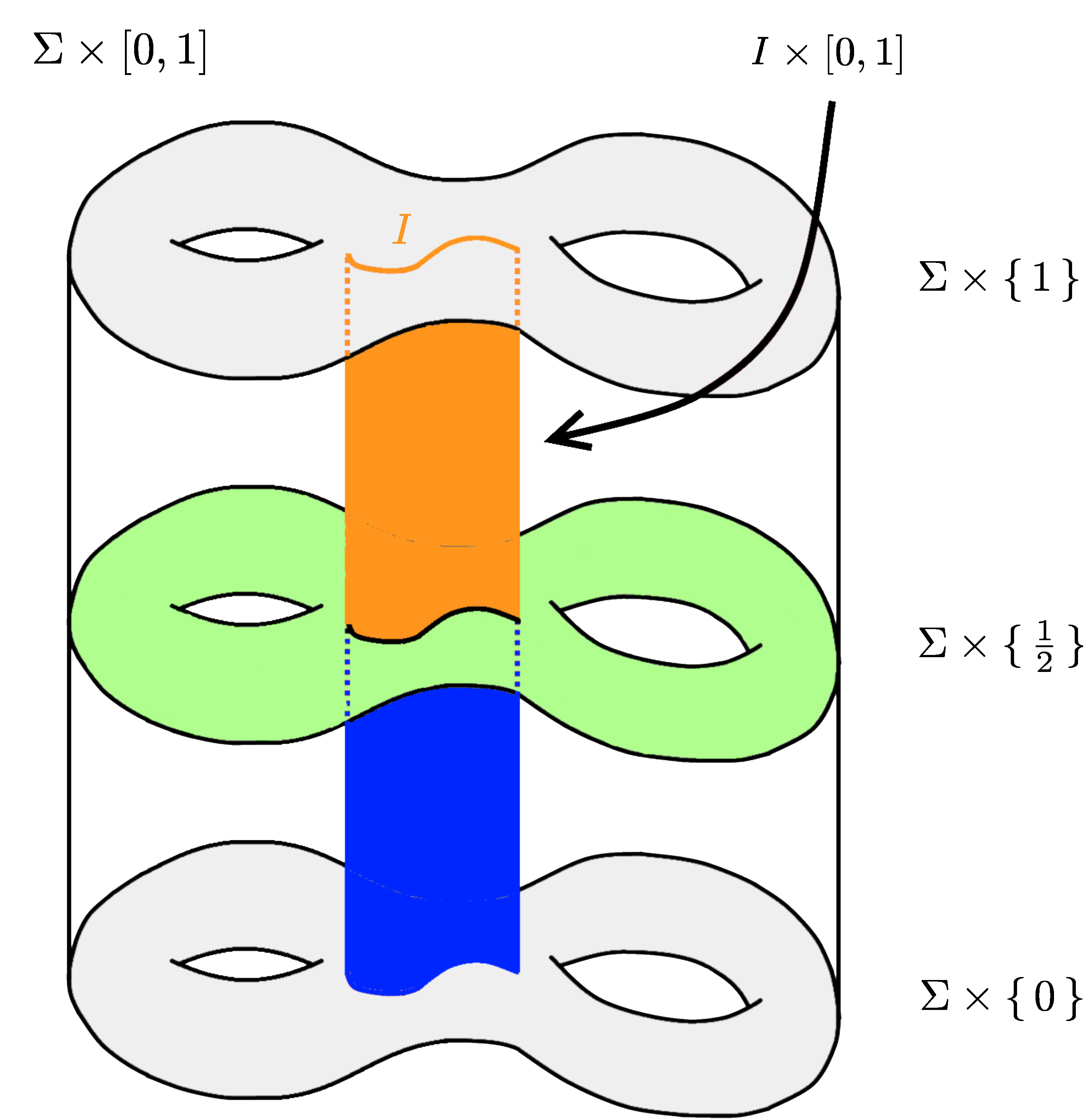
Figure 30. The construction of the Hilbert space $Q(I)$ associated to an interval $I\subset\Sigma$ in the context of the FRS/Kapustin-Saulina construction.

Since we have collars at the ends of our interval, we can smooth out the rectangle $\partial\big{(}I\times[0,1]\big{)}$ to a circle. We will see that the extended cft assigns to $I$ a version of $Q$ modelled on the boundary $\partial\big{(}I\times[0,1]\big{)}$: this is a Hilbert space that looks like $Q$, but which has actions of $\mathcal{A}(J)$ for every $J\subsetneq\partial\big{(}I\times[0,1]\big{)}$, as opposed to $J\subsetneq S^{1}$.

4.2.1. Intermezzo: representations of conformal nets revisited

Before we proceed it is useful to look at a coordinate-independent approach to the representation theory of conformal nets. Consider a circle $S$: a manifold that is diffeomorphic to $S^{1}$, but without a choice of such a diffeomorphism. Let $\text{Rep}_{S}(\mathcal{A})$ denote the category whose objects are Hilbert spaces equipped with compatible actions of $\mathcal{A}(J)$ for every $J\subsetneq S$. $\text{Rep}\,(\mathcal{A})$ is the special case in which $S$ is the unit circle.

Clearly, $\text{Rep}_{S}(\mathcal{A})$ is equivalent to $\text{Rep}\,(\mathcal{A})$, but there is no canonical way of picking such an equivalence. Also, unlike with $\text{Rep}\,(\mathcal{A})$, there is no canonical monoidal structure on $\text{Rep}_{S}(\mathcal{A})$. Instead we have an ‘external product’. Given three circles $S_{1}$, $S_{2}$ and $S_{3}$ with compatible smooth structures as in Figure 31, there is a canonical functor

$$\text{Rep}_{S_{1}}(\mathcal{A})\times\text{Rep}_{S_{2}}(\mathcal{A})\longrightarrow\text{Rep}_{S_{3}}(\mathcal{A})\ .$$

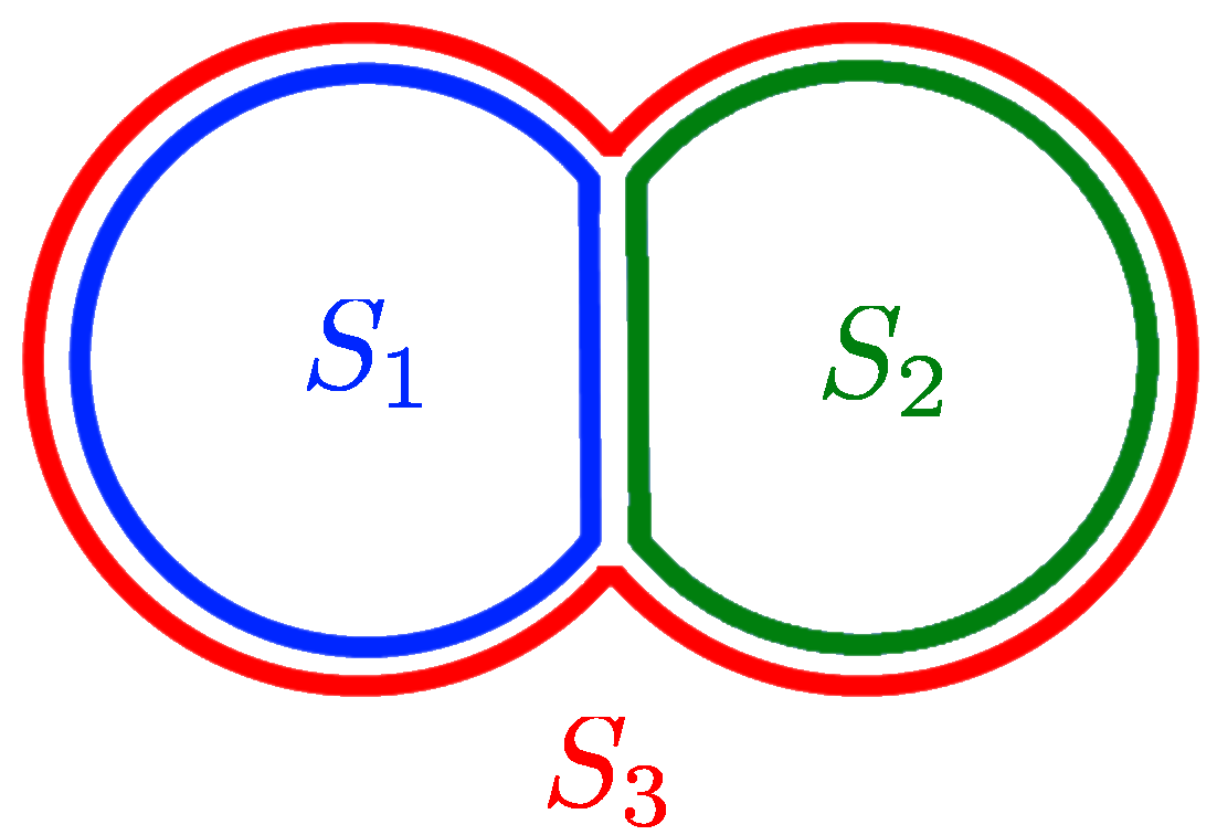
Figure 31. The external product in $\text{Rep}_{S}(\mathcal{A})$ is defined for each triple of circles with compatible smooth structures.

Now, although there is no canonical equivalence between $\text{Rep}_{S}(\mathcal{A})$ and $\text{Rep}\,(\mathcal{A})$, we can nevertheless attempt to construct a functor

$$\text{Rep}\,(\mathcal{A})\longrightarrow\ \text{Rep}_{S}(\mathcal{A})\ ,$$

and see where we fail. Of course, we could just pick a diffeomorphism $S\longrightarrow S^{1}$, but that is clearly non-canonical. Let us try the following

(13) $$H\,\longmapsto\,H\underset{\text{Diff}\,(S^{1})}{\times}\text{Diff}\,(S,\,S^{1})\ ,$$

where $\text{Diff}\,(S,\,S^{1})$ is the set of all diffeomorphisms from $S$ to $S^{1}$, equipped with its natural left action of $\text{Diff}\,(S^{1})$. The reason why there is an action of $\text{Diff}\,(S^{1})$ on $H$ is that whenever a diffeomorphism is supported in a small interval, the corresponding automorphism of $\mathcal{A}(J)$ is inner. Thus, there is an element of that algebra associated to the diffeomorphism, which, in turn, acts on $H$. Those local diffeomorphisms generate $\text{Diff}\,(S^{1})$, and so we get an action of $\text{Diff}\,(S^{1})$.

The reason that (13) does not quite work is that the choice of algebra elements implementing the given inner automorphism is not unique. Indeed, it is only defined up to phase, and therefore the action of $\text{Diff}\,(S^{1})$ on $H$ is only a projective action.

4.2.2. Back to business

We would like to say that the value of the extended full cft on $I$ is the image of $Q\in\text{Rep}\,(\mathcal{A})$ under the functor

$$\text{Rep}\,(\mathcal{A})\longrightarrow\text{Rep}_{\,\partial(I\times[0,1])}\,(\mathcal{A})\ .$$

But, as we have seen, at least at first sight, that does not seem to work. The reason that this nevertheless does work is that $\partial\big{(}I\times[0,1]\big{)}$ has more structure than an arbitrary circle $S$: it has an involution $(x,t)\longmapsto(x,-t)$. Therefore it makes sense to talk about symmetric diffeomorphisms, i.e., those diffeomorphisms that commute with the involution.

Thus, for $S=\partial\big{(}I\times[0,1]\big{)}$, we can replace (13) by

$$\text{Rep}\,(\mathcal{A})\longrightarrow\ \text{Rep}_{S}(\mathcal{A})\ ,\quad H\longmapsto H\underset{\text{Diff}_{\text{sym}}(S^{1})}{\times}\text{Diff}_{\text{sym}}(S,\,S^{1})\ .$$

Now something very nice happens: the universal central extension of $\text{Diff}\,(S^{1})$ splits over $\text{Diff}_{\text{sym}}(S^{1})$, and so that group now does act on $H$, and the formula makes sense. Therefore we can define

(14) $$\text{Rep}\,(\mathcal{A})\longrightarrow\text{Rep}_{\,\partial(I\times[0,1])}\,(\mathcal{A})\ ,\quad Q\longmapsto Q(I)\ .$$

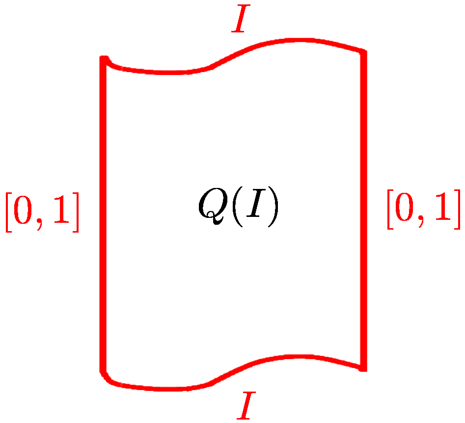
Figure 32. The Hilbert space $Q(I)$ has actions of the copies of $B$ associated to the unit intervals $[0,1]$ on the left and on the right.

To see that $Q(I)$ is indeed a $B$-$B$-bimodule, notice that $A=\mathcal{A}\big{(}[0,1]\big{)}$ has two actions on $Q(I)$, corresponding to the two copies of $[0,1]$ in the boundary of $I\times[0,1]$ (cf. Figure 32). If we identify the boundary $\partial\big{(}I\times[0,1]\big{)}$ with the unit circle via some symmetric diffeomorphism that sends the corners on the left to the ‘north’ and ‘south pole’ of the circle as illustrated in Figure 33, this identifies the left action of $A$ of $Q(I)$ with the standard left action of $A$ on $Q$. Now recall from the proof of Lemma 4.1 that the we have an inclusion $A\subset B$ and that the left action of $A$ on $Q$ extends to an action of $B$ on $Q$ in a canonical way. Therefore, the left action of $A$ of $Q(I)$ extends to an action of $B$.

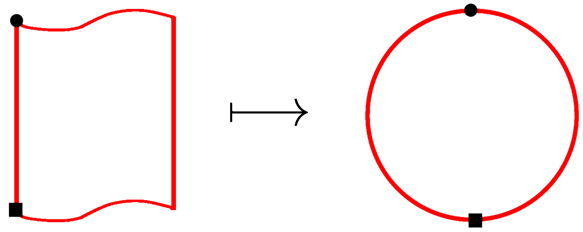
Figure 33. An identification of $\partial\big{(}I\times[0,1]\big{)}$ and a standard circle via a symmetric diffeomorphism mapping the corners on the left to the north and south poles of the circle.

Similarly, with the use of a symmetric diffeomorphism as indicated in Figure 34, we can identify the right action of $\mathcal{A}\big{(}[0,1]\big{)}$ on $Q(I)$ with the standard right action of $A$ on $Q$, which likewise extends to an action of $B$.

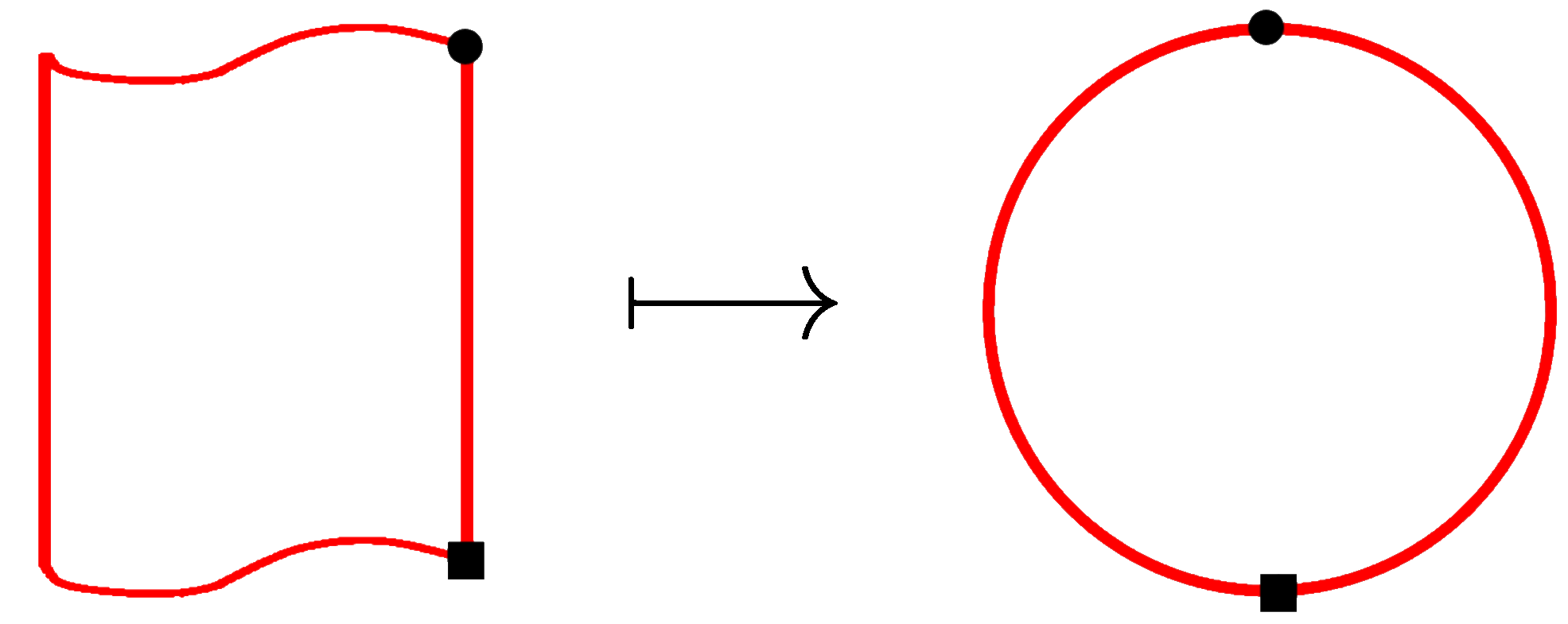
Figure 34. Another identification of $\partial\big{(}I\times[0,1]\big{)}$ and a standard circle, now via a symmetric diffeomorphism sending the corners on the right to the poles of the circle.

At this point it is not too difficult to see, using the fact that $Q\cong L^{2}B$, that the assignment (14) is compatible with glueing:

$${}_{B}Q(I_{1})\,\boxtimes_{B}Q(I_{2})_{B}={}_{B}Q(I_{1}\cup I_{2})_{B}\ .$$

This is of course necessary for our construction to make sense, but it is not very impressive. Let us turn to something more surprising.

4.3. Recovering the state space from the FRS construction

Recall from Section 3.5.2 that the state space (11) of the full cft from the FRS construction is given by

$$H_{\text{full}}\coloneqq\bigoplus_{\mu,\lambda}\text{Hom}_{Q,Q}\big{(}\lambda\boxtimes^{+}Q\boxtimes^{-}\mu^{\vee},Q\big{)}\otimes H_{\lambda}\otimes\overline{H_{\mu}}\ .$$

In this section we will show, or at least sketch, how this result can be reproduced with our construction. The idea is to take the unit circle, cut it in half, and fuse the corresponding algebras over $B\,\bar{\otimes}\,B^{\textup{op}}$. More precisely, we have the following

Theorem 4.2.

Decompose the unit circle as $S^{1}=I\cup J$ such that the intersection $I\cap J$ consists of two points only. Then the fusion of $Q(I)$ with $Q(J)$ over $B\,\bar{\otimes}\,B^{\textup{op}}$ (see Figure 35) is canonically isomorphic to $H_{\textup{full}}$ as a module over the chiral and antichiral algebras.

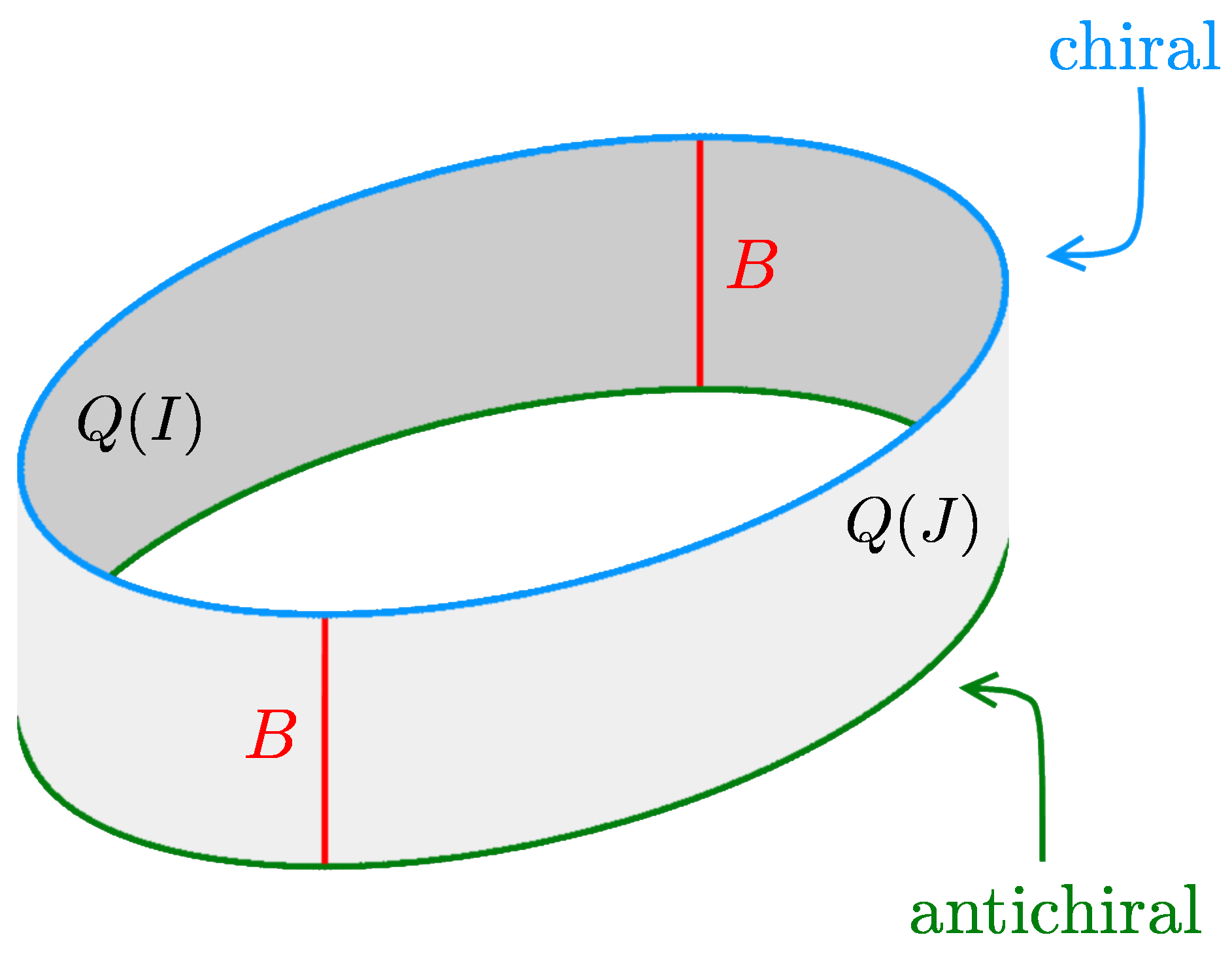
Figure 35. The circle on the top corresponds to the representation of the chiral algebra on $H_{\lambda}$, whilst the circle on the bottom corresponds to the representation of the antichiral algebra on $\overline{H_{\mu}}$. We have used the action of the two copies of the bigger algebra $B$ (recall that $A\subset B$) to fuse $Q(I)$ with $Q(J)$.

For the proof of this theorem we need the following lemma:

Lemma 4.3.

Let $Q$ and $B$ be as in (12), and let $H$ be a module over $A$. Then $H$ is a $Q$-module (i.e. we have a map $Q\boxtimes_{A}H\longrightarrow H$ satisfying the obvious axioms), if and only if it is a $B$-module extending the action of $A$ (i.e. we have a map $B\otimes H\longrightarrow H$ satisfying the obvious axioms).

Similarly, a homomorphism $H_{1}\to H_{2}$ is $Q$-linear iff it is $B$-linear.

With the help of this lemma, Theorem 4.2 can be proved as sketched — literally — in Figure 36.

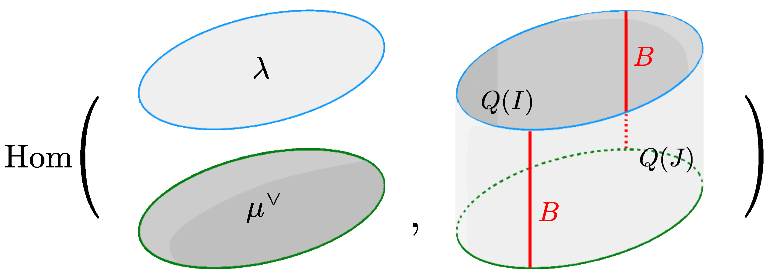
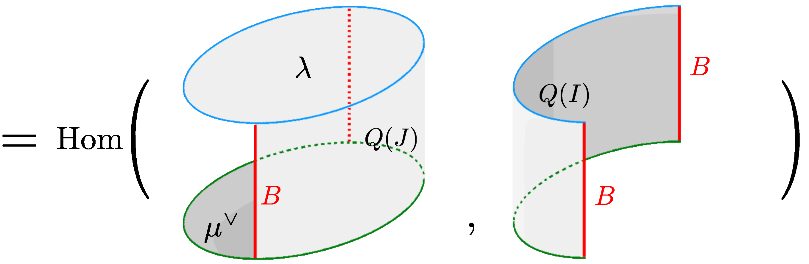
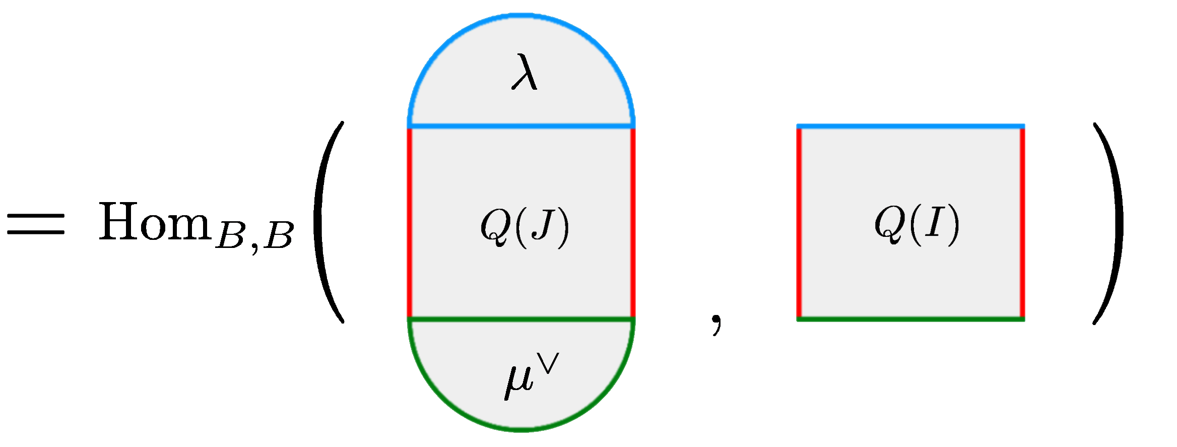
Figure 36. Proof of Theorem 4.2. Depict $\text{Hom}_{Q,Q}\big{(}H_{\lambda}\otimes\overline{H_{\mu}}\,,\,Q(I)\boxtimes Q(J)\big{)}$ as shown on the top. By duality, this is equal to the second line. Now we can flatten the shapes to get to the third line, which corresponds precisely to $\text{Hom}_{Q,Q}\big{(}\lambda\boxtimes^{+}Q\boxtimes^{-}\mu^{\vee},Q\big{)}$. $\square$

4.4. The maps associated to surfaces

Starting from a $\chi$cft and a Frobenius algebra object we have constructed the extended cft corresponding to zero- and one-dimensional manifolds in the source bicategory. To conclude, we mention what happens to two-dimensional surfaces, and show what the open problem is that has to be solved in order to complete our construction.

4.4.1. Discs and surfaces with cusps

It is not too hard to see which bimodule map is associated to a disc with conformal structure. We can view the disc as a cobordism from the empty one-manifold to the bounding circle. Thus, we have to construct a map from $\mathbb{C}$ to the Hilbert space $H_{\text{full}}$ associated to that circle. This is the same as a choice of vector in that Hilbert space. Moreover, this vector should be invariant under the group $PSL_{2}(\mathbb{R})$ of Möbius transformations of the circle. The vacuum vector in $H_{\text{full}}$ is given by $\Omega\otimes\Omega$ in the direct summand $H_{0}\otimes H_{0}$ of $H_{\text{full}}$. Here, $\Omega$ is (also) called the vacuum vector in $H_{0}$, and $H_{0}$ is the vacuum module of the conformal net (the unit object in the category $\text{Rep}\,(\mathcal{A})$). In both cases — i.e. in the case $\Omega\otimes\Omega\in H_{\text{full}}$, and also in the case $\Omega\in H_{0}$ — the vacuum vector is the unique $PSL_{2}(\mathbb{R})$-fixed point up to scalars.

We also have a construction for the bimodule map associated to a surface with two cusps. After a choice of parametrization of the ingoing and outgoing boundaries by the unit interval $[0,1]$, the semigroup $\text{Bigons}\big{(}[0,1]\big{)}$ of bigons (as in (1)) of the unit interval can be identified with the complexification of the group of those diffeomorphisms of $[0,1]$ that leave a neighbourhood of the endpoints fixed.

By extending the action of $\text{Diff}\big{(}[0,1]\big{)}$ in a $\mathbb{C}$-linear fashion to the copy of $\text{Bigons}\big{(}[0,1]\big{)}$ in the chiral sector, and $\mathbb{C}$-antilinearly to the copy of $\text{Bigons}\big{(}[0,1]\big{)}$ in the antichiral sector, we get the desired actions of $\text{Bigons}\big{(}[0,1]\big{)}$.

4.4.2. Open problem: ninja stars

The main open problem is the construction of the bimodule map associated to the ‘ninja star’ depicted in Figure 1. We also have to prove a few basic properties of this map, together with one important relation that is shown in Figure 37.

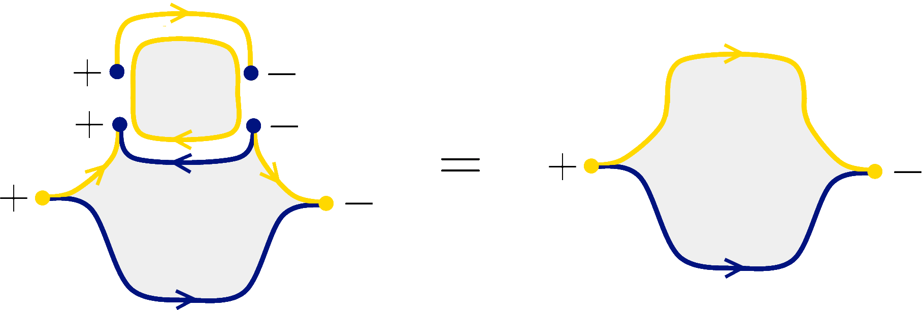
Figure 37. An important relation.

This relation ensures the compatibility between the bimodule map associated to the ninja star (that we want to construct) and the parts of the extended cft that we have already constructed. More precisely, it means the following.

Given the 2-morphism from Figure 38(a) we can form the horizontal composition with the identity 2-morphism on the 1-morphism in Figure 38(b) to get the result in Figure 38(c).

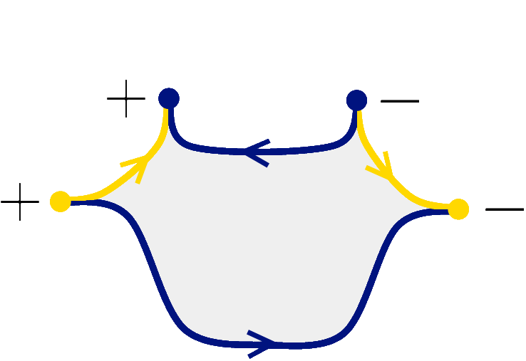
(a) A ninja star.

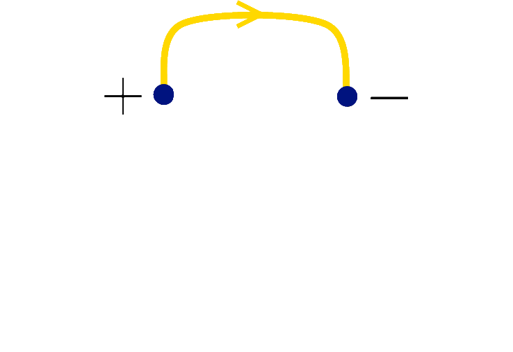
(b) A one-morphism.

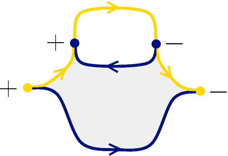
(c) Another 2-morphism.

Figure 38. The 2-morphism on the right is the result of the horizontal compositon of the 2-morphism shown on the left with the identity 2-morphism on the cap in the middle.

The relation drawn in Figure 38(a) describes what should happen if we fill in the hole by vertical composition with the disc, viewed as a 2-morphism as indicated in Figure 39. The disc that we fill in corresponds to the lower two-morphism in Figure 40.

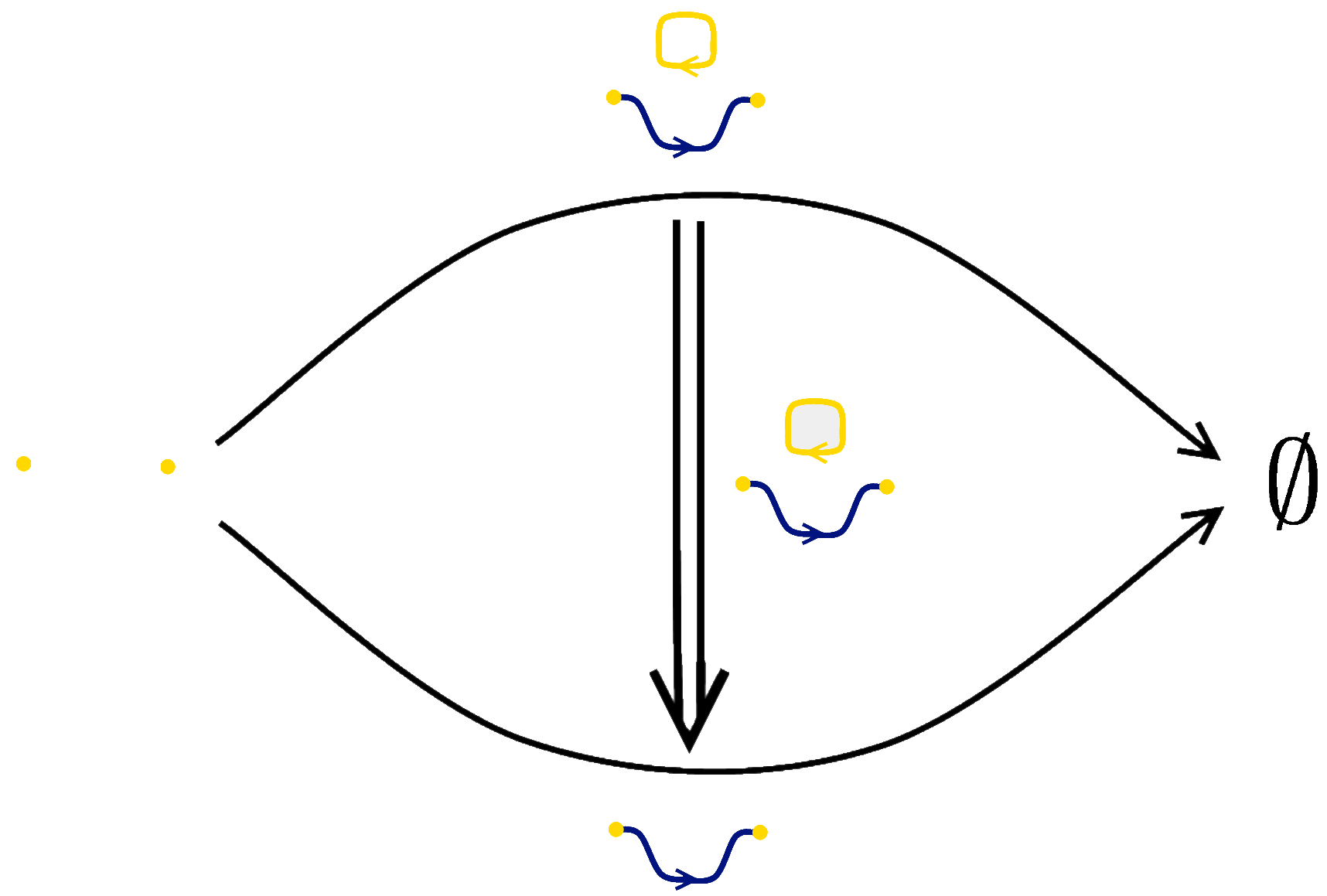
Figure 39. The relation from Figure 37 involves a horizontal composition with the tensor product of the 2-morphism corresponding to the disc and the identity 2-morphism on the (blue) 1-morphism.

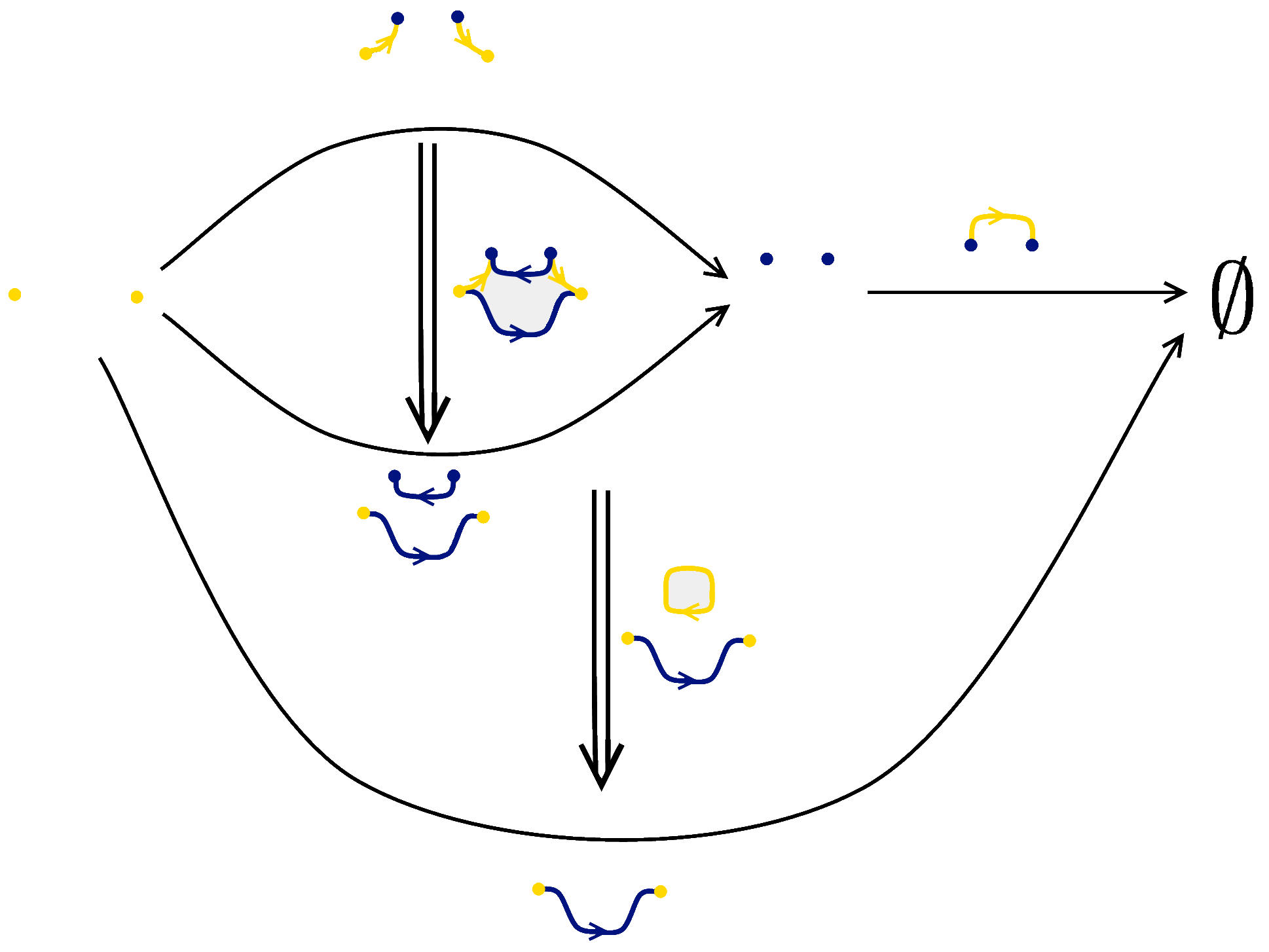
Figure 40. The diagram showing the objects, 1-morphisms and 2-morphism featuring in the important relation from Figure 37.

Now, any surface can be decomposed into discs and ninja-stars via a simple algorithm: draw closed curves with transverse intersections on the surface, and then replace those intersections by ninja stars (see Figure 41). Given the bimodule map associated to the ninja star and the relation from Figure 37, this decomposition should allow one to construct the full extended cft from it.

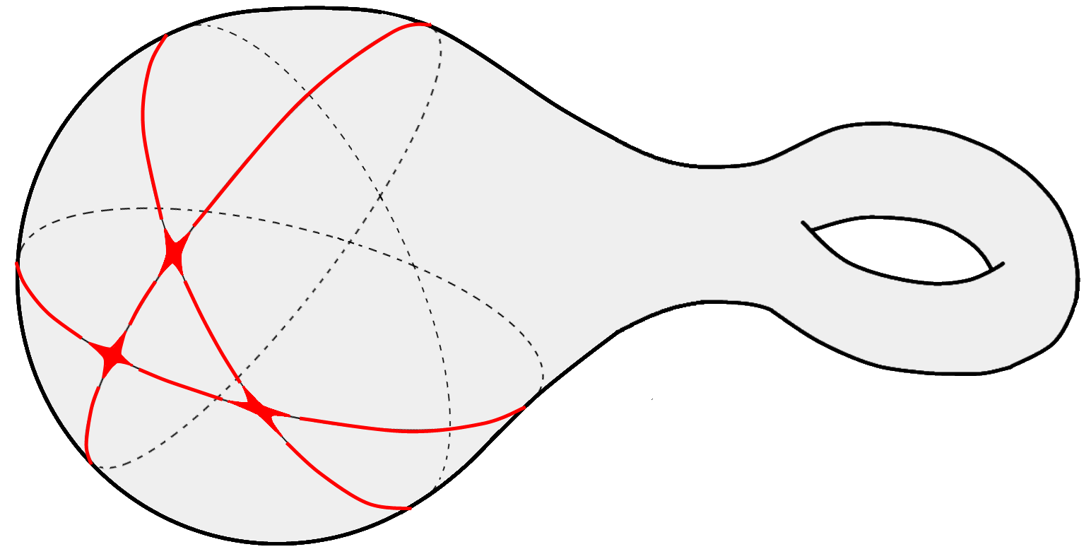
Figure 41. By drawing closed curves on a 2-surface and replacing their junctions by ninja stars, every surface can be decomposed into discs, ninja stars, and intervals.

References

- [Ati89] M. Atiyah, Topological quantum field theories, Inst. Hautes Études Sci. Publ. Math. 68 (1989), 175–186.
- [BDH09] A. Bartels, C. Douglas, and A. Henriques, Conformal nets and local field theory, 2009, arXiv:0912.5307.
- [BDH13] A. Bartels, C.L. Douglas, and A. Henriques, Conformal nets I: coordinate-free nets, arXiv:1302.2604, 2013.
- [Bel90] S. Bell, Mapping problems in complex analysis and the -problem, Bull. Amer. Math. Soc. 22 (1990), 233–259.
- [Ben67] B. Jean, Introduction to bicategories, Reports of the Midwest Category Seminar, Springer Berlin, 1967, pp. 1–77.
- [CIZ87] A. Cappelli, C. Itzykson, and J.-B. Zuber, Modular invariant partition functions in two dimensions, Nuclear Phys. B 280 (1987), no. 3, 445–465.
- [Fre93] D.S. Freed, Extended structures in topological quantum field theory, Quantum topology (Dayton), 1993, pp. 162–173.
- [FRS02] J. Fuchs, I. Runkel, and C. Schweigert, TFT construction of RCFT correlators. I. Partition functions, Nuclear Phys. B 646 (2002), no. 3, 353–497.
- [FRS04a] by same author, TFT construction of RCFT correlators. II. Unoriented world sheets, Nuclear Phys. B 678 (2004), no. 3, 511–637.
- [FRS04b] by same author, TFT construction of RCFT correlators. III. Simple currents, Nuclear Phys. B 694 (2004), no. 3, 277–353.
- [FRS05] by same author, TFT construction of RCFT correlators. IV. Structure constants and correlation functions, Nuclear Phys. B 715 (2005), no. 3, 539–638.
- [FRS06] by same author, TFT construction of RCFT correlators. V. Proof of modular invariance and factorisation, Theory Appl. Categ. 16 (2006), no. 16, 342–433.
- [GF93] F. Gabbiani and J. Fröhlich, Operator algebras and conformal field theory, Comm. Math. Phys. 155 (1993), no. 3, 569–640.
- [Haa75] U. Haagerup, The standard form of von Neumann algebras, Math. Scand. 37 (1975), no. 2, 271–283. MR 0407615 (53 #11387)
- [Hua97] Y.-Z. Huang, Two-dimensional conformal geometry and vertex operator algebras, Progress in Mathematics, vol. 148, Birkhauser Boston, Inc., 1997.
- [KL04a] Y. Kawahigashi and R. Longo, Classification of local conformal nets. Case , Ann. of Math. (2) 160 (2004), no. 2, 493–522. MR 2123931 (2006i:81119)
- [KL04b] by same author, Classification of two-dimensional local conformal nets with and 2-cohomology vanishing for tensor categories, Comm. Math. Phys. 244 (2004), no. 1, 63–97. MR 2029950 (2005d:81228)
- [KS11] A. Kapustin and N. Saulina, Surface operators in 3d topological field theory and 2d rational conformal field theory, Mathematical foundations of quantum field theory and perturbative string theory, Proc. Sympos. Pure Math., vol. 83, Amer. Math. Soc., 2011, arXiv:1012.0911v1 [hep-th], pp. 175–198.
- [Lon08] R. Longo, Lectures on conformal nets II, 2008, http://www.mat.uniroma2.it/~longo/Lecture%20Notes.html.
- [LR04] R. Longo and K.-H. Rehren, Local fields in boundary conformal QFT, Rev. Math. Phys. 16 (2004), no. 7, 909–960.
- [Lur09] Jacob Lurie, On the classification of topological field theories, Current developments in mathematics, 2008, Int. Press, Somerville, MA, 2009, pp. 129–280. MR 2555928 (2010k:57064)
- [Ost03] V. Ostrik, Module categories, weak Hopf algebras and modular invariants, Transform. Groups 8 (2003), no. 2, 177–206.
- [Pos03] H. Posthuma, Quantization of Hamiltonian loop group actions, Ph.D. thesis, 2003.
- [RS06] D. Radnell and E. Schippers, Quasisymmetric sewing in rigged Teichmüller space, Commun. Contemp. Math. 8 (2006), no. 4, 481–534.
- [Seg] G. Segal, Sewing Riemann surfaces together, (unpublished preprint).
- [Seg88] by same author, The definition of conformal field theory, Differential geometrical methods in theoretical physics (Como, 1987), NATO Adv. Sci. Inst. Ser. C Math. Phys. Sci., vol. 250, Kluwer Acad. Publ., 1988, pp. 165–171.
- [Seg04] by same author, Topology, geometry and quantum field theory, London Math. Soc. Lecture Note Ser., vol. 308, ch. The definition of conformal field theory, pp. 421–577, Cambridge Univ. Press, 2004.
- [Seg07] by same author, Elliptic cohomology, London Math. Soc. Lecture Note Ser., vol. 342, ch. What is an elliptic object?, pp. 306–317, Cambridge Univ. Press, 2007.
- [ST04] S. Stolz and P. Teichner, Topology, geometry and quantum field theory, London Math. Soc. Lecture Note Ser., vol. 308, ch. What is an elliptic object?, pp. 247–343, Cambridge Univ. Press, 2004.
- [TL97] V. Toledano Laredo, Fusion of Positive Energy Representations of , Ph.D. thesis, University of Cambridge, 1997, arXiv:math/0409044 [math.OA].
- [TUY89] A. Tsuchiya, K. Ueno and Y. Yamada, Conformal field theory on universal family of stable curves with gauge symmetries. Integrable systems in quantum field theory and statistical mechanics, 459–566, Adv. Stud. Pure Math., 19, Academic Press, Boston, MA, 1989.
- [Was98] A. Wassermann, Operator algebras and conformal field theory. III. Fusion of positive energy representations of using bounded operators, Invent. Math 133 (1998), no. 3, 467–538.
- [Xu00] F. Xu, Jones-Wassermann subfactors for disconnected intervals, Commun. Contemp. Math. 2 (2000), no. 3, 307–347.
- [Zhu96] Y. Zhu, Modular Invariance of Characters of Vertex Operator Algebras, J. Amer. Math. Soc. 9 (1996), 237–302.