Multiscale enhanced path sampling based on the Onsager-Machlup action: Application to a model polymer

Abstract

We propose a novel path sampling method based on the Onsager-Machlup (OM) action by generalizing the multiscale enhanced sampling (MSES) technique suggested by Moritsugu and coworkers (J. Chem. Phys. 133, 224105 (2010)). The basic idea of this method is that the system we want to study (for example, some molecular system described by molecular mechanics) is coupled to a coarse-grained (CG) system, which can move more quickly and computed more efficiently than the original system. We simulate this combined system (original + CG system) using (underdamped) Langevin dynamics where different heat baths are coupled to the two systems. When the coupling is strong enough, the original system is guided by the CG system, and able to sample the configuration and path space more efficiency. We need to correct the bias caused by the coupling, however, by employing the Hamiltonian replica exchange where we prepare many path replica with different coupling strengths. As a result, an unbiased path ensemble for the original system can be found in the weakest coupling path ensemble. This strategy is easily implemented because a weight for a path calculated by the OM action is formally the same as the Boltzmann weight if we properly define the path “Hamiltonian”. We apply this method to a model polymer with Asakura-Oosawa interaction, and compare the results with the conventional transition path sampling method.

I Introduction

Molecular dynamics (MD) simulation MDbook1 ; MDbook2 is a rigorous and versatile approach for investigating dynamic trajectory of molecular systems by numerical integration of Newton’s equation. Its applicability has been quickly expanded in time and length scales owing to the development of hardwares (general purpose ones such as PC clusters, GPGPU, supercomputers, or special purpose ones such as Anton Anton ), convenient softwares with reliable force fields (Amber amber , Gromacs gromacs , CHARMM charmm , NAMD namd and others), and efficient numerical algorithms MDbook2 . However, because the MD step size should be close to the vibrational time scales of the molecular system ($\sim$ 1fs), conventional MD simulations have not been applicable to processes that are extremely rare, slow, and/or diffusive processes. While the MD simulation is able to explore fast structural fluctuations around a basin of potential (or free) energy surface, it often fails to sample interbasin hopping, which describes various phenomena such as protein folding and chemical reactions TPS ; TPS2 .

To overcome this problem, several methods have been proposed and tested over the last two decades (for reviews, see TPS3 ; FFMK09 ). One of the pioneering works is transition path sampling (TPS) developed by Chandler, Dellago, Bolhuis and coworkers TPS ; TPS2 ; TPS3 . Since then, there has been effort to improve the efficiency of TPS calculations, such as transition interface sampling (TIS) TIS and partial TIS PPTIS . Related to these methods are milestoning milestone and forward flux sampling FFsampling . Studies on further improvement of the efficient path sampling is still under way.

An alternative approach to path sampling is the action-based methods such as the Onsager-Machlup (OM) action method Wiegelbook ; Zuckermanbook . The OM action has been used for path search problems by Elber and coworkers EGC02 , Eastman and coworkers EGD01 , and Orland and coworkers Orland09 . In the early works, this method has been used to find the most dominant pathway, but recent advances have made it possible to explore the ensemble of paths MBFO11 . For instance, an efficient path sampling has been proposed previously FSK10 with the use of temperature replica exchange HN96 ; Hansmann97 ; SO99 . The computational advantage of the action-based methods is that the time step for the action integral can be taken to be as large as 100 fs (or more), which is much larger than a typical MD step ($\simeq$ 1fs). Moreover, it is straightforward to carry out such calculations in parallel with respect to each time step and each path. This will certainly match the advantage of recent computational environment with hyper-parallel architectures such as GPGPU and supercomputer. Because of these computational demands, the ensemble of paths has not been easily obtained, but the fluctuations of paths as well as configurations should be important for biomolecules, which is worth pursuing to understand biological functions.

In this paper, we suggest to enhance the efficiency of the OM action-based path sampling using the multiscale enhanced sampling (MSES) devised by Moritsugu and coworkers MTK10 . The MSES method has been successfully applied to the calculation of free energy profiles of a small peptide (chignolin) MTK10 , intrinsically disordered protein (sortase) MTK12a , and a protein-protein complex MTK12b . In the original MSES, the system of interest is the canonical ensemble for the atomistic degrees of freedom, which will be called “MM DoF”. We assume a coupling between the MM DoF and a reference coarse-grained DoF, which will be called “CG DoF”, mimicking the typical behavior of the MM DoF in an economical manner. The total Hamiltonian of the combined system is defined as

$$H=H_{\rm MM}+H_{\rm CG}+\lambda H_{\rm MMCG}$$ (1)

where $H_{\rm MM},H_{\rm CG}$ and $\lambda H_{\rm MMCG}$ represent the Hamiltonians of the MM and CG DoF, and the interaction between the MM and CG DoF, respectively.

Assuming that the CG DoF is able to move around the CG configuration space quickly, the MM DoF will be dragged accordingly for a finite value of $\lambda$, which leads to an efficient search of the MM configurations. However, our goal is to obtain the canonical ensemble with respect to MM-DoF, which is proportional to $\exp(-\beta H_{\rm MM})$, in the absence of the MM-CG interaction, i.e. $\lambda=0$. To meet both of these ends, we use the Hamiltonian replica exchange HRE among the combined MM-CG systems with different $\lambda$ values. In other words, we simulate a replicated set of the combined MM-CG systems with $\lambda_{1}>\lambda_{2}\cdots\lambda_{N_{\rm rep}}$, where $N_{\rm rep}$ is the number of replicas, and they are exchanged from time to time according to the Metropolis criterion MDbook2 . We then collect the MM ensemble with the smallest $\lambda_{N_{\rm rep}}$ (ideally $\lambda_{N_{\rm rep}}=0$), which should be equal to the unbiased canonical MM ensemble.

Using the OM action-based methods, we can do the same as above: We consider an extended system where MM and CG DoF are coupled, and the OM action for the coupled system is defined as

$$S=S_{\rm MM}+S_{\rm CG}+\lambda S_{\rm MMCG}$$ (2)

where $S_{\rm MM},S_{\rm CG}$ are the OM actions for the MM and CG DoF, and $\lambda S_{\rm MMCG}$ the interaction between them. Using $\lambda$ as the exchange parameter, the “canonical weight” for a MM path $\propto\exp(-\beta S_{\rm MM})$ can be retrieved with the same logic as above. Note that in the formulation of MSES there is a subtle issue concerning the nonequilibrium nature of the combined system due to the coupling to different temperatures MTK10 , but this problem is circumvented by using the idea of “scaling” (see Appendix C). As shown below, when we only use the “conventional” OM method for the MM DoF (without any coupling to the CG DoF), we need a longer computation time for statistical convergence. Hence it is indispensable to use this type of method to enhance path sampling, especially when dealing with large molecular systems.

This paper is organized as follows. In Sec. II, we introduce the Onsager-Machlup action principle and formulate the multiscale enhanced sampling for path space using the OM action (MSES-OM). We also mention the model polymer system devised by Micheletti and coworkers TMCM06 ; MBL08 , which is employed in the following calculations. In Sec. III, we investigate the numerical performance of the MSES-OM method using the model polymer. We also examine the numerical accuracy of the method by comparing with the results using the conventional transition path sampling. In Sec. IV, we summarize the paper and discuss the further aspects of the MSES-OM method.

II Formulation

II.1 Onsager-Machlup action for multi-dimensional systems

Let us consider the case where the dynamics of the MM system is described by an overdamped Langevin equation,

$$\dot{x}_{\alpha}=-\frac{1}{\gamma}_{\alpha}\frac{\partial U}{\partial x_{\alpha}}+\sqrt{2D_{\alpha}}\eta_{\alpha}(t)$$ (3)

where $x_{\alpha}$ is mass-weighted coordinates, $U$ a potential energy, $\gamma_{\alpha}$ an intrinsic friction coefficient, $D_{\alpha}$ an diffusion coefficient, and $\eta_{\alpha}(t)$ a Gaussian-white noise satisfying $\langle\eta_{\alpha}(t)\eta_{\alpha^{\prime}}(t^{\prime})\rangle=\delta_{\alpha\alpha^{\prime}}\delta(t-t^{\prime})$. As Eq. (3) is a stochastic differential equation, the dynamics is characterized by the probability (“weight”) of generating a path (or trajectory) $x(t)$. According to Onsager and Machlup OM1 ; OM2 , the weight is proportional to $\exp(-\beta S[x(t)])$ where $S[x(t)]$, which is called the Onsager-Machlup (OM) action, is a functional of $x(t)$. In numerical calculations, the OM action is approximated by its discretized form as

$$S[x(t)]=\frac{\Delta U}{2}+\sum_{i=1}^{N_{\rm bead}-1}\left[\sum_{\alpha=1}^{M}\frac{\omega_{\alpha}^{2}}{2}(x_{\alpha,i+1}-x_{\alpha,i})^{2}+V_{\rm eff}(\{x_{\alpha,i}\})\right]$$ (4)

where $N_{\rm bead}$ is the number of discretized segments of a path, or “beads”, $M$ the number of the MM DoF (usually $3\times$ number of atoms), $\Delta U=U(x_{\rm fin})-U(x_{\rm ini})$ the potential difference between the initial and final states, and the effective “potential” is defined as

$$V_{\rm eff}(\{x_{\alpha}\})\equiv\sum_{\alpha=1}^{M}\left[\frac{1}{8\omega_{\alpha}^{2}}U_{x_{\alpha}}^{2}-\frac{k_{B}T}{4\omega_{\alpha}^{2}}U_{x_{\alpha}x_{\alpha}}\right]$$ (5)

with

$$\omega_{\alpha}=\sqrt{\frac{\gamma_{\alpha}}{2\Delta t_{\rm OM}}}.$$ (6)

This is an effective frequency determined by the friction and the time interval for the path discretization $\Delta t_{\rm OM}$. Here we used the notations $U_{x}$ and $U_{xx}$ to represent the first and second derivatives of $U$ with respect to $x$.

To sample path space using the above OM action, we have employed the position-Verlet MDbook1 ; MDbook2 type scheme to integrate the Langevin equations, i.e.,

$$\tilde{x}_{\alpha,i} = x_{\alpha,i}+\frac{p_{\alpha,i}}{\tilde{m}_{i}}\frac{\Delta\tau}{2},$$ (7)

$$p_{\alpha,i}^{\prime} = (1-\tilde{\gamma}\Delta\tau/2)p_{\alpha,i}-\left.\frac{\partial S}{\partial x_{\alpha,i}}\right|_{x_{\alpha,i}=\tilde{x}_{\alpha,i}}\Delta\tau+\sqrt{2\tilde{\gamma}k_{B}T\tilde{m}_{i}\Delta\tau}R_{\alpha,i}(t),$$ (8)

$$x_{\alpha,i}^{\prime} = \tilde{x}_{\alpha,i}+\frac{p_{\alpha,i}^{\prime}}{\tilde{m}_{i}}\frac{\Delta\tau}{2},$$ (9)

where $p_{\alpha,i}$, $\tilde{m}_{i}$, $\tilde{\gamma}$ are the fictitious momenta, mass, and friction coefficient, which are similar to those for the imaginary-time path integral simulations Tuckermanbook . $R_{i}(t)$ is the Gaussian random variable with zero average and unit variance. Note that the time step to integrate the above equations of motion $\Delta\tau$ has nothing to do with the time step for the discretization of the OM action $\Delta t_{\rm OM}$. The numerical integration of these equations result in the canonical distribution $\exp(-\beta S)$. However, if the path space is huge, which is usually the case for complex systems, an efficient algorithm to sample the path space is required to reduce the computational load. This is the reason why we will introduce the MSES method MTK10 ; MTK12a ; MTK12b .

II.2 Multiscale enhanced sampling for path space

In the formulation of MSES MTK10 , Moritsugu et al. introduced several replicas with different coupling parameters $\lambda_{1},\lambda_{2},\cdots$, and exchange $m$-th and $n$-th parameters during the simulation of the combined system according to the probability

$$p_{mn}=\min(1,\exp\Delta_{mn})$$ (10)

where

$$\Delta_{mn}=\beta(\lambda_{m}-\lambda_{n})(H_{{\rm MMCG},m}-H_{{\rm MMCG},n})$$ (11)

and $\beta$ is the inverse temperature of the MM DoF. This is an application of the Hamiltonian replica exchange method HRE to the combined MM-CG system. The MM canonical ensemble is obtained from that of the combined MM-CG system with the smallest $\lambda$.

This formalism can be immediately applied to the problem of path sampling using the OM action. In this case the exchange probability is determined by

$$\Delta_{mn}=\beta(\lambda_{m}-\lambda_{n})(S_{{\rm MMCG},m}-S_{{\rm MMCG},n})$$ (12)

where the interaction OM action can be chosen as

$$S_{\rm MMCG}=\frac{1}{2}\sum_{i=1}^{N^{\rm CG}_{\rm bead}}(\theta_{i}(\{x_{\alpha,i}\})-x_{i}^{\rm CG})^{2}$$ (13)

where $\theta_{i}$ represents collective variables calculated from MM DoF $\{x_{\alpha,i}\}$, $x_{i}^{\rm CG}$ is the corresponding CG variables, and $N^{\rm CG}_{\rm bead}$ is the number of beads to discretize the CG path. The schematic picture of our MSES-OM method is shown in Fig. 1. The basic strategy here is that the CG variables (blue, upper) move rather freely in path space to “guide” the MM variables (red, lower).

Here it is important to notice on the scaling of the number of replicas required as the system size increases. As emphasized by Moritsugu et al. MTK10 , the interaction “Hamiltonian” scales with the number of CG DoF not with that of MM DoF because it contains only CG DoF and the projected MM DoF onto the CG space. Hence this method does not suffer from the problems caused by the number of MM DoF as in the case of temperature replica exchange Hansmann97 ; SO99 . Furthermore, in this study, the number of CG beads is smaller than that of MM beads, i.e., $N^{\rm CG}_{\rm bead}$ (=240) is ten times smaller than $N_{\rm bead}$ (=2400), reducing the cost of calculations.

In order for MSES to work efficiently, the CG DoF must move quickly and dominate the dynamics of the combined system. This situation is achieved, for example, when the total mass of the CG system is comparable to or larger than the MM system and the temperature of the CG system is much higher than that of the MM system. We thus take the CG mass $=20m_{0}$ and CG temperature $=80k_{B}T$, whereas $m_{0}$ is the “bead” mass of the model polymer (see Appendix A) and the temperature for the MM DoF is $k_{B}T\simeq 300$K. (Note that this CG mass is not a real mass because this is just introduced to carry out the “artificial” OM dynamics for the CG DoF.) Because two different temperatures are set for the MM and CG DoF, the resulting ensemble seems to exhibit a strongly nonequilibrium behavior. However, the desired information can be retrieved from the ensemble with the smallest coupling parameter $\lambda_{N_{\rm rep}}$. The subtle point to use different temperatures for the MM and CG DoF are summarized in Appendix C.

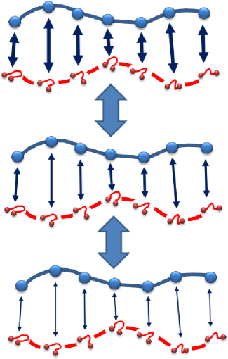
Figure 1: Schematic picture of the proposed multiscale enhanced sampling for path space using the OM action (MSES-OM). The blue (red) beads represent CG (MM) DoF, and the arrows between them with different thickness represent different interaction strengths. The thick arrows between the combined MM-CG systems schematically represent “exchange” due to Hamiltonian replica exchange (actually the coupling parameters are exchanged).

II.3 Model polymer

In this section, we briefly explain the model system we use for path sampling, which is a coarse-grained polymer studied by Micheletti and coworkers TMCM06 . The potential energy of this model, $U_{1}+U_{2}+U_{3}$, consists of the Asakura-Oosawa (AO) type interaction $U_{3}$ and the finitely extensible elastic chain $U_{1}+U_{2}$,

$$U_{1} = \epsilon_{1}\sum_{i<j}e^{-a(r_{ij}-r_{ij}^{0})},$$ (14)

$$U_{2} = -\epsilon_{2}\sum_{i}\ln\left[1-\left(\frac{r_{i,i+1}}{1.5r_{i,i+1}^{0}}\right)^{2}\right],$$ (15)

$$U_{3} = -\frac{\phi k_{B}T}{16r^{3}}\sum_{i<j}\left(2\tilde{r}_{ij}+3r_{ij}-\frac{3\delta_{ij}^{2}}{r_{ij}}\right)\tilde{r}_{ij}^{2}\Theta(\tilde{r}_{ij}),$$ (16)

where $\tilde{r}_{ij}=2r+r_{ij}^{0}-r_{ij}$, $\delta_{ij}=|R_{i}-R_{j}|$, $r_{ij}^{0}=R_{i}+R_{j}$, $\Theta(x)$ is the Heaviside function (=1 for $x\geq 0$ and 0 for $x<0$), and the friction coefficient is given by

$$\gamma_{i}=6\pi\eta R_{i}(1+2.5\phi).$$ (17)

The parameter values we employ here are almost the same as in the original paper TMCM06 except that we made $a$ parameter four times larger, that is, we used a softer core.

Micheletti et al. used the AO interaction to model the crowding effect due to RNA and proteins in a cell, and studied the (un)looping kinetics of the model polymer by changing the size of the system. They found that the mean-first passage time (MFPT) for the unlooping dynamics does not depend on the size of the system, whereas the MFPT for the looping dynamics does. In this paper, we employ the smallest number of beads (five), and study the unlooping dynamics, which takes place with $\sim$ 3 $\mu$s time scale TMCM06 .

For path sampling using the OM action, we need to evaluate the effective potential defined in Eq. (5) and its derivatives because we use the equations of motion, Eqs. (7)-(9). Because there are only two-body interactions in $U_{1}+U_{2}+U_{3}$, this is easily evaluated analytically. On the other hand, for path sampling using the conventional transition path sampling (TPS), we integrate the overdamped Langevin equation (3) for this model from many different initial paths.

Although this is a coarse-grained model, in this paper, we call this model as an “atomistic” model or MM DoF because our purpose here is to illustrate our method. The CG DoF coupled to this MM DoF will be introduced just below.

II.4 CG model for the model polymer and the CG variable

For the MSES-OM method, we need to introduce CG variables and its OM action. For the model polymer introduced above, we take the conventional end-to-end distance $z$ as a CG variable, and the “potential” function is introduced as

$$U^{\rm CG} = \alpha\left[\frac{U_{1}^{\rm CG}+U_{2}^{\rm CG}}{2}-\sqrt{\left(\frac{U_{1}^{\rm CG}-U_{2}^{\rm CG}}{2}\right)^{2}+\epsilon^{2}}\right],$$ (18)

$$U_{1}^{\rm CG} = \frac{1}{2}k_{1}(z-z_{1})^{2}+v_{1},$$ (19)

$$U_{2}^{\rm CG} = \frac{1}{2}k_{2}(z-z_{2})^{2}+v_{2},$$ (20)

which is a conventional empirical valence-bond type potential MTK10 . In the previous study, it is shown that this “single” order parameter can nicely describe the unlooping process of the model polymer TMCM06 , so we also use this single variable as the CG DoF. The values of the CG parameters are summarized in Appendix B.

III Results

III.1 Numerical stability of OM dynamics

It is known that the model polymer described in Sec. II.3 has two free energy minima with respect to the end-to-end distance (this is a basic observation when we build a CG model in Sec. II.4), one at the looped configuration, $z=24$ nm, and the other at the unlooped configuration, $z=45$ nm. There is a barrier between them, which are characterized by the barrier height with $\simeq$ 0.4 kcal/mol (looped to barrier top) and $\simeq$ 0.9 kcal/mol (barrier top to unlooped). In order to study the unlooping process, the starting point of the OM path is fixed at $z=24$ nm while the end point is made free to move around $z=45$ nm (see Fig. 4). From an independent molecular dynamics run, it has been confirmed that we need the trajectory of about 30 $\mu$s to get the information on the barrier crossing. Therefore, the length of OM path has been taken to be $N_{\rm bead}\Delta t_{\rm OM}\simeq 40\ \mu$s where the OM step size and the number of beads are taken as $\Delta t_{\rm OM}=10\ t_{0}\simeq 16$ ns (with $t_{0}$ being the unit of time scale, see Appendix A) and $N_{\rm bead}=2400$, respectively. The value of $\Delta t_{\rm OM}$ may be taken as small as possible, but due to our experience $\Delta t_{\rm OM}$ is reasonably small as long as the fluctuation of the action is balanced between the bead spring and potential contributions, i.e. each in the second term in the right hand side of Eq. (4). We find the sampling procedure unstable when taking $\Delta t_{\rm OM}$ too large, say $\Delta t_{\rm OM}=1000\ t_{0}$, when the fluctuation of the potential contribution is much larger than that of the bead spring contribution.

III.2 Interaction between MM and CG DoF

Next we show the effect of the coupling between CG and MM paths. In Fig. 2, several CG (red) and MM (green) paths during the OM dynamics are drawn with two different coupling parameters: $\lambda=10^{-2}$ (left) and $\lambda=10^{-5}$ (right). We can see that the MM path follows the CG path in the strong coupling case (left), while the MM path is more independent from the CG path in the weak coupling case (right).

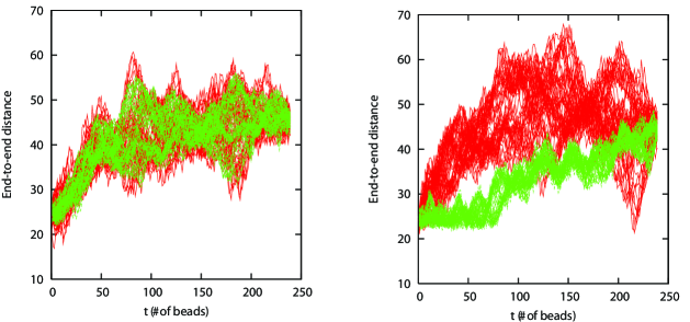
Figure 2: The end-to-end distance as a function of time (or number of beads) calculated from the OM dynamics for MM (green) and CG (red) DoF with the strong (left) and weak (right) coupling cases. We overlay 10 “snapshots” from each OM dynamics. There are 10 times difference in the MM and CG beads numbers, so every one of 10 beads is shown for the MM DoF.

For a closer analysis on the correlation between MM and CG paths, we define the root mean square displacement (RMSD) between the MM and CG DoF as

$$\delta_{\rm MMCG}=\sqrt{\frac{1}{N^{\rm CG}_{\rm bead}}\sum_{i=1}^{N^{\rm CG}_{\rm bead}}(\theta_{i}(\{x_{\alpha,i}\})-x^{\rm CG}_{i})^{2}}=\sqrt{\frac{2S_{\rm MMCG}}{N^{\rm CG}_{\rm bead}}}.$$ (21)

The histograms for this quantity over 10⁶ OM steps are shown in Fig. 3 for different coupling strengths ($\lambda$’s). We take 6 different values of $\lambda_{i}$ between 10^-2 and 10^-5: $\lambda_{i}=0.01\times 0.25^{i-1}$ ($i=1,\cdots,6$) for 6 different replicas. For the largest $\lambda=\lambda_{1}$ (=10^-2), $\delta_{\rm MMCG}$ fluctuates around $\sim$ 7, but for the smallest $\lambda=\lambda_{6}$ (=10^-5), the distribution spreads from 5 to 50, indicating that the correlation is small between the MM and CG DoF. From this figure, we assume that the paths with $\lambda_{6}$ is close to those with null coupling ($\lambda=0$), because the two distributions with $\lambda_{5}$ and $\lambda_{6}$ are almost the same.

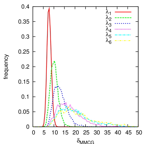
Figure 3: The distribution function of the root mean square displacement between the MM and CG DoF as defined in Eq. (21) for different coupling strengths. Note that we never used Hamiltonian replica exchange here.

III.3 First passage time distribution and comparison to TPS

We carried out a MSES-OM calculation with 10⁶ OM steps. The path data were saved every 100 OM steps, and 10⁴ data sets were collected. In the MSES-OM calculation, the replica exchange was attempted every 10 OM steps, and the acceptance ratio was found to be about 30 %. In Fig. 4, we show the overlay of snapshots of 100 OM paths from the calculation. The time course is indicated by arrows, and the “time difference” between the neighboring snapshots is about 4 $\mu$s, corresponding to 240 beads. We can see that the distribution of paths grows during the time course, but it is hard to tell what is happening here.

Figure 4: Unbiased path ensemble calculated by the MSES-OM method. A hundred of OM trajectories are superimposed, indicating the fluctuation of the path ensemble. The “time difference” between the neighboring snapshots is about 4 $\mu$s, corresponding to 240 beads.

In Fig. 5, we show the time evolution of the distribution with respect to the distances between “beads” $i$ and $j$ denoted by $x_{ij}$. For comparison, we also showed the result using the conventional OM calculation without Hamiltonian replica exchange, which is called “single OM” in the figure. We can see that during the transition the end-to-end distance, $x_{15}$, is broadly distributed among the two basins (middle-bottom panel). In contrast, the distances distributions for $x_{13}$ and $x_{35}$ are already close to those at the final time, indicating that these variables, $x_{13}$ and $x_{35}$, first equilibrate before the end-to-end distance does. The difference between the single OM and MSES-OM methods is found in the distributions for $x_{15}$ and $x_{25}$ during the transition. This clearly shows the efficiency of our MSES-OM method over the single OM method for path sampling.

Finally we show the first passage time distribution (FPTD) in Fig. 6 HCB10 ; ZJZ07 . This is defined as a histogram of the elapsed times in moving from one place to the other. In this work we monitor the end-to-end distance $z=x_{15}$ and measure the time interval where the system evolves from $z_{1}=28$ to $z_{2}=35$, which correspond to two locations before and after the barrier crossing (not free energy minima) ZJZ07 . We can see that the barrier crossing occurs most likely in 2 $\mu$s, and completes within 35 $\mu$s. In order to have a converged result for Fig. 6, we repeated the MSES-OM calculation 10 times from different initial conditions, so the number of path in the ensemble is 10⁵.

As a reference, we have also carried out TPS calculations using the Crooks-Chandler algorithm CC01 for the same system. As can be seen, the FPTD is in reasonable agreement with the MSES-OM result. To obtain Fig. 6, we used 100 independent TPS runs with 10⁴ TPS steps each. The data is saved every 10 TPS steps, and 10⁵ data sets are collected in total. Thus, the amount of data for TPS calculation and the MSES-OM calculation is comparable. The statistical accuracy in Fig. 6 seems to be similar between the MSES-OM and TPS methods, at least for the present system.

However, the comparison of computational effort is difficult in general, since the OM methods requires the higher-order derivatives of the potential whereas the parallelized calculation can be done efficiently. We can at least say that OM method would be of use in studying slow and diffusive processes such as conformational changes of large molecules and protein folding. There should be much room for further improvement of the OM method such as the dominant pathway Orland09 , the discretization in length EGC02 , and the use of the efficient hessian calculation EH08 .

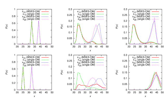
Figure 5: Distribution functions for different distances, $x_{13},x_{35}$ for the upper panel and $x_{15},x_{25}$ for the lower panel, of the model polymer calculated by the single OM and the MSES-OM method. The left, middle, and right panels correspond to the distributions at $t=0$, $1233\Delta t_{\rm OM}$, and $2323\Delta t_{\rm OM}$, respectively.

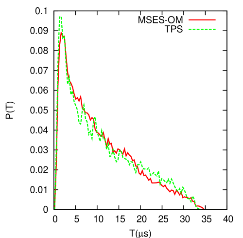
Figure 6: First passage time distributions (FPTDs) for the model polymer calculated by TPS (green) and by the MSES-OM method (red).

IV Concluding remarks

To efficiently sample huge path space of complex systems, in this paper we proposed a multiscale path sampling method based on the Onsager-Machlup (OM) action combined with multiscale enhanced sampling (MSES). We applied this MSES-OM method to a model polymer with the Asakura-Oosawa interaction, and showed the effectiveness of our method, which is comparable to conventional transition path sampling (TPS) with many initial paths.

We have shown that the MSES method can be easily combined with the OM action. This is because the ensemble of stochastic paths subject to overdamped Langevin equation is isomorphic to the canonical ensemble of a polymer of beads connected by harmonic springs. Note that the path obtained by the OM or MSES-OM method contains the nonequilibrium information such as the first passage time for barrier crossing. This is conceptually different from the thermodynamic analysis of barrier crossing, i.e., transition state theory based on the free energy landscape. In order to apply this method to complex molecular systems, which is obviously the next step, it is indispensable to make a great use of parallel calculation techniques. For a future work, the authors are interested in studying the conformational change of adenylate kinase MFTFMK12 , for which the minimum free energy path was recently elucidated by the on-the-fly string method ME07 .

Another direction to pursue is the Baysian-type inference of the model parameters using the OM action MBL08 ; Harada . It is known that the formulation of the dynamic data assimilation data_assimilation is almost the same as our MSES-OM method, where the CG DoF corresponds the direct variables to be observed, and the MM DoF to the hidden variables of the system studied. Hence the MSES-OM formalism should be used for the parameter estimation of general dynamical system problems.

Finally we mention a possible extension of this approach to quantum systems. Since the centroid variable of a quantum particle has been used in TPS AS09 and in the string method SF12 , we expect that we can use the centroid variable in the OM-action based methods as well. This will be an extension of the OM path sampling based on the Feynman-Hibbs formula which was recently suggested by Faccioli and coworkers BGF11 ; BF12 .

Appendix A Units for dimensionless variables

We here summarize the dimensionless units which were used in this paper. We convert all the variables (mass, length, energy, time, friction coefficient) into dimensionless ones by choosing

$$m_{0} = \rho\cdot\frac{4}{3}\pi R^{3}=\frac{4}{3}\pi\times 1.35\,{\rm g/cm}^{3}\times(12.5\,{\rm nm})^{3}=1.10\times 10^{-20}\,{\rm kg},$$ (22)

$$l_{0} = 10^{-9}\,{\rm m}=1\,{\rm nm},$$ (23)

$$\epsilon_{0} = k_{B}T=1.38\times 10^{-23}\,{\rm J/K}\times 300\,{\rm K},\simeq 4.14\times 10^{-21}\,{\rm J},$$ (24)

$$t_{0} = l_{0}\sqrt{\frac{m_{0}}{\epsilon_{0}}}=1.63\times 10^{-9}\,{\rm s}=1.63\,{\rm ns},$$ (25)

$$\gamma_{0} = m_{0}/t_{0}=6.75\times 10^{-12}\,{\rm kg/s}.$$ (26)

The order of the friction coefficient is given by

$$\gamma_{i} = 6\pi\eta R_{i}=6\pi\times 0.05\times 10^{-3}\,{\rm g/cm/s}\times 12.5\,{\rm nm}$$ (27)

$$\simeq 1.18\times 10^{-9}\,{\rm kg/s}=175\gamma_{0}.$$

If we take as a time step for the Langevin dynamics: $\Delta t=t_{0}/100=16.3$ ps, which is a reasonable choice, the jump magnitude due to the random force is

$$\sqrt{\frac{2k_{B}T}{\gamma_{i}}\Delta t}=\Delta L\simeq 0.01\,{\rm nm}$$ (28)

which seems to be reasonable as well for this model polymer system.

Appendix B Parameters for models and simulations

B.1 Parameters for the MM DoF

The parameters used for the model polymer defined in Eqs. (14)-(16) are $a=4\,{\rm nm}^{-1},\epsilon_{1}=0.24\epsilon_{0},\epsilon_{2}=70\epsilon_{0},r=2.5\,{\rm nm},\phi=0.15,R_{i}=12.5\,{\rm nm},\eta=5\,{\rm cP},\rho=1.35\,{\rm g/cm}^{3}$, which are the same as in TMCM06 except the value of $a$.

B.2 Parameters for the CG DoF

The parameters used for the CG model defined in Eqs. (18)-(20) are $k_{1}=0.8,k_{2}=0.02,z_{1}=24,z_{2}=46,v_{1}=3.5,v_{2}=-2.0,\epsilon=5.0,\alpha=0.7$. The parameters for the OM action are $\Delta t_{\rm OM}^{\rm CG}=100,\zeta^{\rm CG}=333,D^{\rm CG}=0.003,N^{\rm CG}_{\rm bead}=240$ such that the total duration becomes the same as the MM case and $k_{B}T=1.0=D\zeta$. (However, this matching of the timescales for both DoF might not be necessary.) The value of the diffusion constant $D=0.003$ was a little bit smaller than that of Fig. 4 in MBL08 . In any case, we can estimate this value from a short-time simulation.

Appendix C On the use of different temperatures for MM and CG DoFs

At first sight, if we use different temperatures coupled to different parts of the system, the system is in a nonequilibrium state which cannot be described by the canonical distribution. This is the case in our path ensemble as well as the configuration ensemble in the original paper of MSES MTK10 . However, this problem can be bypassed in the following way.

Because the formalism is the same for both configuration and path sampling, we employ the original setting for configuration sampling. For simplicity we consider only a two-dimensional case with CG variables $(Q,P)$ and MM variables $(q,p)$, but this can be easily generalized.

We set the total (combined) Hamiltonian as

$$H = H_{\rm MM}(q,p)+H_{\rm CG}(Q,P)+V_{\rm MMCG}(q,Q)$$ (29)

$$= \frac{p^{2}}{2m}+V_{\rm MM}(q)+\frac{P^{2}}{2M}+V_{\rm CG}(Q)+V_{\rm MMCG}(q,Q)$$

where $m,M$ are masses for MM and CG DoF. To realize the canonical distribution for the total system, we consider the underdamped Langevin dynamics. The equations for the original variables are

$$\frac{dp}{dt} = -\gamma_{\rm MM}p-\frac{\partial V_{\rm MM}}{\partial q}-\lambda\frac{\partial V_{\rm MMCG}}{\partial q}+\sqrt{2\gamma_{\rm MM}mk_{B}T_{\rm MM}}\eta_{\rm MM}(t),$$ (30)

$$\frac{dP}{dt} = -\gamma_{\rm CG}P-\frac{\partial V_{\rm CG}}{\partial Q}-\lambda\frac{\partial V_{\rm MMCG}}{\partial Q}+\sqrt{2\gamma_{\rm CG}Mk_{B}T_{\rm MM}}\eta_{\rm CG}(t),$$ (31)

where $\gamma_{*}$ is the friction coefficient and $\eta_{*}(t)$ is the Gaussian white noise. Note that we used the same temperature $T_{\rm MM}$ to realize the canonical distribution for the total system $\propto e^{-H/k_{B}T_{\rm MM}}$.

Changing the CG variables from $(Q,P)$ to $(\tilde{Q},\tilde{P})$, which are defined by

$$\tilde{Q}=\sqrt{\alpha}Q,\tilde{P}=P/\sqrt{\alpha},$$ (32)

with $\alpha=T_{\rm MM}/T_{\rm CG}$ ($\leq 1$), the Langevin equation for the CG variable becomes

$$\frac{d\tilde{P}}{dt}=-\gamma_{\rm CG}\tilde{P}-\frac{\partial V_{\rm CG}}{\partial\tilde{Q}}-\lambda\frac{\partial V_{\rm MMCG}}{\partial\tilde{Q}}+\sqrt{2\gamma_{\rm CG}Mk_{B}T_{\rm CG}}\eta_{\rm CG}(t).$$ (33)

Note that the temperature is $T_{\rm CG}$ in this equation instead of $T_{\rm MM}$.

To have the same $\alpha$ scaling for the terms proportional to $\lambda$ (the third terms in Eqs. (30), (31), (33) on the right hand side), the interaction Hamiltonian has to be

$$V_{\rm MMCG}(q,Q)=\frac{\lambda}{2}(\theta(q)-\sqrt{\alpha}{Q})^{2}$$ (34)

where $\theta(q)$ represents the transformation from the MM variable to a collective one.

Hence the above total Hamiltonian can be recast into

$$H=H_{\rm MM}(q,p)+\frac{\tilde{P}^{2}}{2\tilde{M}}+V_{\rm CG}(\tilde{Q}/\sqrt{\alpha})+V_{\rm MMCG}(q,\tilde{Q}/\sqrt{\alpha})$$ (35)

with $\tilde{M}=M/\alpha$. As a result, by simulating Eqs. (30) and (33) with different temperatures, $T_{\rm MM}$ and $T_{\rm CG}$, we can achieve the canonical distribution for the total system with a single temperature $T_{\rm MM}$. In actual calculations, we use only $\tilde{Q}$ space to construct the CG model, $\tilde{V}_{\rm CG}(\tilde{Q})\equiv V_{\rm CG}(\tilde{Q}/\sqrt{\alpha})$, and the interaction is $\tilde{V}_{\rm MMCG}(q,\tilde{Q})\equiv V_{\rm MMCG}(q,\tilde{Q}/\sqrt{\alpha})=\frac{\lambda}{2}(\theta(q)-\tilde{Q})^{2}$, it is reasonable to take $\tilde{V}_{\rm CG}(\tilde{Q})$ which can mimic the original free energy landscape calculated from $V_{\rm MM}(q)$.

References

- (1) M.P. Allen and D.J. Tildesley, Computer Simulation of Liquids, Oxford Science, Oxford (1987).
- (2) D. Frenkel and B. Smit, Understanding Molecular Simulation: From Algorithms to Applications, 2nd ed., Academic Press (2002).
- (3) J.L. Klepeis, K. Lindorff-Larsen, R.O. Dror, and D.E. Shaw, Curr. Opin. Struc. Biol. 19, 120-127 (2009); R.O. Dror, R.M. Dirks, J.P. Grossman, H. Xu, and D.E. Shaw, Annu. Rev. Biophys. 41, 429 (2012).
- (4) http://ambermd.org/
- (5) http://www.gromacs.org/
- (6) http://www.charmm.org/
- (7) http://www.ks.uiuc.edu/Research/namd/
- (8) C. Dellago, P.G. Bolhuis, and P.L. Geissler, Adv. Chem. Phys. 123, 1-78 (2002).
- (9) C. Dellago and P.G. Bolhuis, Top. Curr. Chem. 268, 291-317 (2007).
- (10) C. Dellago and P.G. Bolhuis, Adv. Poly. Sci. 221, 167 (2008).
- (11) S. Fuchigami, H. Fujisaki, Y. Matsunaga, and A. Kidera, Adv. Chem. Phys. 145, 35 (2011).
- (12) T.S. van Erp, D. Moroni, and P.G. Bolhuis, J. Chem. Phys. 118, 7762 (2003); T.S. van Erp and P.G. Bolhuis, J. Comp. Phys. 205, 157 (2005).
- (13) D. Moroni, T.S. van Erp, and P.G. Bolhuis, J. Chem. Phys. 120, 4055 (2004).
- (14) T. Faradjian and R. Elber, J. Chem. Phys. 120, 10882 (2004); A.M.A. West, R. Elber. and D. Shalloway, J. Chem. Phys. 126, 145104 (2007).
- (15) R.J. Allen, D. Frenkel, and P.R. ten Wolde, J. Chem. Phys. 124, 024102 (2004); R.J. Allen, D. Frenkel, and P.R. ten Wolde, J. Chem. Phys. 124, 194111 (2004).
- (16) F.W. Wiegel, Introduction to Path-Integral Methods in Physics and Polymer Science, World Scientific, Singapore (1986).
- (17) D.M. Zuckerman, Statistical Physics of Biomolecules: An Introduction, CRC Press (2010).
- (18) R. Elber, A. Ghosh, and A. Cardenas, Acc. Chem. Res. 35, 396 (2002).
- (19) P. Eastman, N. Gronbech-Jensen, and S. Doniach, J. Chem. Phys. 114, 3823 (2001).
- (20) P. Faccioli, M. Sega, F. Pederiva, and H. Orland, Phys. Rev. Lett. 97 (2006) 108101; M. Sega, P. Faccioli, F. Pederiva, G. Garberoglio, and H. Orland, ibid. 99 (2007) 118102; E. Autieri, P. Faccioli, M. Sega, F. Pederiva, and H. Orland, J. Chem. Phys. 130, 064106 (2009).
- (21) G. Mazzola, S.a Beccara, P. Faccioli, and H. Orland, J. Chem. Phys. 134, 164109 (2011).
- (22) H. Fujisaki, M. Shiga, and A. Kidera, J. Chem. Phys. 132, 134101 (2010).
- (23) K. Hukushima and K. Nemoto, J. Phys. Soc. Jpn. 65, 1604 (1996).
- (24) U.H.E. Hansmann, Chem. Phys. Lett. 281, 140-150 (1997).
- (25) Y. Sugita and Y. Okamoto, Chem. Phys. Lett. 314, 141-151 (1999).
- (26) K. Moritsugu, T. Terada, and A. Kidera, J. Chem. Phys. 133, 224105 (2010).
- (27) K. Moritsugu, T. Terada, and A. Kidera, J. Am. Chem. Soc. 134, 7094 (2012).
- (28) K. Moritsugu, T. Terada, and A. Kidera, unpublished.
- (29) H. Fukunishi, O. Watanabe, and S. Takada, J. Chem. Phys. 116, 9058 (2002).
- (30) N.M. Toan, D. Marenduzzo, P.R. Cook, and C. Micheletti, Phys. Rev. Lett. 97, 178302 (2006).
- (31) C. Micheletti, G. Bussi, and A. Laio, J. Chem. Phys. 129, 074105 (2008).
- (32) L. Onsager and S. Machlup, Phys. Rev. 91, 1505 (1953).
- (33) S. Machlup and L. Onsager, Phys. Rev. 91, 1512 (1953).
- (34) M.E. Tuckerman, Statistical Mechanics: Theory and Molecular Simulation, Oxford University Press (2010).
- (35) Z. Hu, L. Cheng and B.J. Berne, J. Chem. Phys. 133, 034105 (2010).
- (36) B.W. Zhang, D. Jasnow, and D.M. Zuckerman, Proc. Nat. Acad. Sci. USA, 104, 18043 (2007).
- (37) G.E. Crooks and D. Chandler, Phys. Rev. E 64, 026109 (2001).
- (38) E. Vanden-Eijnden and M. Heymann, J. Chem. Phys. 128, 061103 (2008).
- (39) Y. Matsunaga, H. Fujisaki, T. Terada, T. Furuta, K. Moritsugu, and A. Kidera, PLoS Comput. Biol. 8, e1002555-1-12 (2012).
- (40) L. Maragliano and E. Vanden-Eijnden, Chem. Phys. Lett. 446, 182 (2007).
- (41) M. Miyazaki and T. Harada, J. Chem. Phys. 134, 085108 (2011).
- (42) A. Apte, M. Hairer, A.M. Stuart, and J. Voss, Physica D 230, 50 (2007).
- (43) D. Antoniou and S.D. Schwartz, J. Chem. Phys. 131, 224111 (2009).
- (44) M. Shiga and H. Fujisaki, J. Chem. Phys. 136, 184103 (2012).
- (45) S. a Beccara, G. Garberoglio, and P. Faccioli, J. Chem. Phys. 135, 034103 (2011).
- (46) L. Boninsegna and P. Faccioli, J. Chem. Phys. 136, 214111 (2012).