Extrinsic Spin Hall Effect Induced by Resonant Skew Scattering in Graphene

Abstract

We show that the extrinsic spin Hall effect can be engineered in monolayer graphene by decoration with small doses of adatoms, molecules, or nanoparticles originating local spin-orbit perturbations. The analysis of the single impurity scattering problem shows that intrinsic and Rashba spin-orbit local couplings enhance the spin Hall effect via skew scattering of charge carriers in the resonant regime. The solution of the transport equations for a random ensemble of spin-orbit impurities reveals that giant spin Hall currents are within the reach of the current state of the art in device fabrication. The spin Hall effect is robust with respect to thermal fluctuations and disorder averaging.

The spin Hall effect (SHE) Dyakonov71 ; Hirsch99 ; Zhang00 ; Jungwirth12 , that is, the appearance of a transverse spin current in a nonmagnetic conductor by pure electrical control, has been predicted to occur in materials with large spin-orbit coupling (SOC). Over the last decade, its study has lead to an intense experimental activity Kato04 ; Sih06 ; Ando12 ; Valenzuela06 ; Seki08 , due to its potential application in spintronics. Recently, the SHE has been explored for replacing ferromagnetic metals with spin injectors in applications Liu11 ; Liu12 , opening the door to the development of spintronic devices without magnetic components.

The activation and control of spin-polarized currents is both of fundamental and technological interest. The SHE could be used for an efficient conversion of charge current into spin-polarized currents. The ratio of the spin Hall current to the steady-state charge current, commonly known as the spin Hall angle $\theta_{\textrm{sH}}$, measures this efficiency and it is the most important figure of merit for practical applications. Generally speaking, the SHE in metals and semiconductors originates from (i) extrinsic mechanisms, which are due to spin-dependent scattering of charge carriers by impurities in the presence of SOC Dyakonov71 ; Hirsch99 ; Zhang00 , and (ii) intrinsic mechanisms, entirely due to SOC in the electronic band structure, which occur in the absence of any scattering process. In semiconductors, the spin Hall angles are in the range of $0.0001-0.001$ Kato04 ; Ando12 . On the other hand, $\theta_{\textrm{sH}}$ for metals can be considerably larger, being of the order of $0.01$ for Pt Morota11 and $0.1$ in a recent measurement performed in Ta Liu12 .

Since its successful isolation, graphene graphene has also become the subject of intensive study in spintronics Tombos07 ; Cho07 ; Han11 ; Avsar11 ; Dlubak12 . In this material, electrons can propagate ballistically and the carrier density and polarity can be controlled by an external gate. Spin-orbit and hyperfine interactions are extremely weak in graphene and therefore the spin coherence length is expected to be long Hernando06 ; Fabian09 . These characteristics make graphene appealing for passive spintronic applications, e.g., as a high-fidelity channel for spin-encoded information Persin12 . A striking possibility is to modify graphene for active spintronics. This may be achieved via spin-orbit splitting of the band dispersion, e.g., by bringing heavy metallic atoms in close contact to graphene Marchenko12 , or by locally inducing sizeable SOC ($\sim 10$ meV) ahcn08 ; weeks11 . In Ref. ahcn08 , distortions induced by covalently bonded impurities were predicted to produce the desired effect, and Ref. [weeks11, ] suggests local SOC enhancement via tunneling of electrons in and out of a heavy atom. Phenomenologically, random spin-orbit fields have also been predicted to generate nonzero $\theta_{\textrm{sH}}$ RandomSOC . Moreover, it has been proposed that, in the presence of SOC, graphene could exhibit the quantum spin Hall effect Kane06 .

In this Letter, we consider a monolayer of graphene decorated by a small density of impurities generating a spin-orbit interaction in their surroundings. We show that a robust SHE develops through asymmetric (skew) scattering events. Crucially, and unlike two-dimensional electron gases (2DEGs), for which resonant enhancement of skew scattering Raikh08 requires resorting to fine tuning and sometimes to phenomena such as the Kondo effect Hewson_Book ; Nagaosa09 , our proposal takes advantage of graphene being an atomically thin membrane, whose local density of states easily resonates with several types of adatoms, molecules, or nanoparticles. Resonant scatterers have been predicted to play an important role in charge transport at high electronic densities ResScatt ; Ferreira11 . Here, we argue that a similar physics is behind a huge potential of graphene for the extrinsic SHE. The decoration with small doses of certain particles only partially suppresses the charge carrier mobilities of graphene devices, which combined with large spin diffusion lengths and Fermi energy tunability, makes this material a promising candidate for spintronic integrated circuits with SHE-based spin-polarized current activation and control.

According to our calculations, the extrinsic spin Hall effect in graphene, as that recently reported in hydrogenated graphene samples Balakrishnan13 , can originate from skew scattering alone. The latter is absent in the first Born approximation Ballantine and, therefore, we compute transport relaxation rates nonperturbatively via exact partial-wave expansions. Our results indicate that functionalized graphene can deliver spin Hall angles comparable to those found in pure metals ($\theta_{\textrm{sH}}\sim 0.01-0.1$ Morota11 ; Ando12 ; Kato04 ).

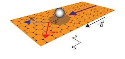
Figure 1: Schematic picture of extrinsic spin Hall effect generated by transport skewness. An impurity (sphere) near the graphene sheet causes a local spin-orbit field with range $R$. The scattering of components with positive (negative) angular momentum is enhanced (suppressed) for charge carriers with $s_{z}=1$ ($s_{z}=-1$), resulting in a net spin Hall current.

In order to investigate the extrinsic SHE and its dependence on Fermi energy and temperature, we consider a continuum model of graphene decorated with a small concentration of impurities that locally generate SOC over nanometer-size regions. The latter could be metallic nanoparticles inducing SOC via the proximity effect, but other physical realizations are also possible. (In fact, adatoms in graphene often cluster due to ripples Rappoport09 or due to a low adsorption energy Kawakami10 .)

Our starting point is the continuum-limit Hamiltonian of graphene ${\cal H}_{0}=\hbar v_{F}(\tau_{z}\sigma_{x}p_{x}+\sigma_{y}p_{y})$, where $\mathbf{p}=(p_{x},p_{y})$ is the 2D kinematic momentum operator around one of the two inequivalent Dirac points $K$ and $K^{\prime}$, $v_{F}\approx 10^{6}$ m/s is the Fermi velocity, and $\boldsymbol{\sigma}$ and $\boldsymbol{\tau}$ denote Pauli matrices, with $\sigma_{z}=\pm 1$ [$\tau_{z}=\pm 1$] describing states on the A(B) sublattice [at $K$($K^{\prime}$)]. The spin-orbit splitting in the band structure of pristine graphene is of the order of 10 $\mu$eV and therefore can be safely neglected Fabian09 . The large scatterers considered here induce sizeable local SOC of the intrinsic-type ${\cal V}_{\textrm{SO}}^{(I)}=\Delta_{I}(\mathbf{r})\tau_{z}\sigma_{z}s_{z}$ and/or Rashba-type ${\cal V}_{\textrm{SO}}^{(R)}=\Delta_{R}(\mathbf{r})(\tau_{z}\sigma_{x}s_{y}-\sigma_{y}s_{x})$; here, $\mathbf{s}$ are Pauli matrices for spin and $\mathbf{r}=(x,y)$ is the charge carrier position. The dependence of $\mathcal{V}_{\textrm{SO}}^{(I)}$ in the spin and orbital operators is the same as the SOC in flat, pristine graphene. On the other hand, ${\cal V}_{\textrm{SO}}^{(R)}$ originates in perturbations breaking mirror symmetry about the graphene’s plane (e.g., single-site adsorption). The impurity potentials are assumed to be smooth on the lattice scale and thus sublattice symmetry breaking terms (crucial in the single adatom limit Gmitra13 ) are not considered here. For such large scatterers intervalley scattering is negligible and, in the long wavelength limit, assuming that potentials have radial symmetry, the scatterer is described by

$${\cal V}_{\textrm{ad}}(r)=\mathcal{V}_{\textrm{SO}}(r)+V_{0}(r),$$ (1)

where $r=|\mathbf{r}|$, and the (spin-independent) electrostatic potential $V_{0}(r)$ accounts for extra scalar scattering. Thus, for $r\gg R$, where $R$ is the range of the potential $\mathcal{V}_{\textrm{ad}}$, the wave function around the $K$ point reads

$$|\psi_{\lambda,\mathbf{k}}(\mathbf{r})\rangle=\left(\begin{array}[]{c}1\\ \lambda\end{array}\right)e^{ikr\cos\theta}|s\rangle+\frac{f_{\lambda}^{ss}(\theta)}{\sqrt{-ir}}\left(\begin{array}[]{c}1\\ \lambda e^{i\theta}\end{array}\right)e^{ikr}|s\rangle+\frac{f_{\lambda}^{s\bar{s}}(\theta)}{\sqrt{-ir}}\left(\begin{array}[]{c}1\\ \lambda e^{i\theta}\end{array}\right)e^{ikr}|\bar{s}\rangle\ ,$$ (2)

where $\lambda=\pm 1$ indicates the carrier polarity with energy $\epsilon=\lambda\hbar v_{F}k$, the ket $|s=\pm\rangle$ describes the orientation of the spin along the $z$ axis, perpendicular to the graphene plane ($\bar{s}\equiv-s$); $f_{\lambda}^{ss}(\theta)$ and $f_{\lambda}^{s\bar{s}}(\theta)$ are the elastic and inelastic (“spin-flip”) scattering amplitudes at scattered angle $\theta$, respectively. The latter is related to the $T$ matrix satisfying the Lippmann-Schwinger equation $\mathcal{T}(\epsilon)=\mathcal{V}_{\textrm{ad}}+\mathcal{V}_{\textrm{ad}}G_{0}(\epsilon)\mathcal{T}(\epsilon)$, where $G_{0}(\epsilon)$ is the Green’s function $G_{0}(\epsilon)=\left(\epsilon-\mathcal{H}_{0}+\lambda i0^{+}\right)^{-1}$. Thus, $f_{\lambda}^{ss^{\prime}}(\theta)\equiv f_{\lambda,KK}^{ss^{\prime}}(\theta)$ and $f_{\lambda,\tau\tau^{\prime}}^{ss^{\prime}}(\theta)\propto\langle\lambda\mathbf{k}s\tau|\mathcal{T}(\epsilon)|\lambda\mathbf{p}s^{\prime}\tau^{\prime}\rangle$ with $\tau,\tau^{\prime}=K,K^{\prime}$, $k=|\mathbf{k}|=|\mathbf{p}|$, and $\theta=\angle(\mathbf{k},\mathbf{p})$.

Let us denote as $\mathcal{F}_{\lambda}(\mathbf{k},\mathbf{p})$ the $4\times 4$ matrix whose elements are $f_{\lambda,\tau\tau^{\prime}}^{ss^{\prime}}(\theta)$ in the spin and valley subspace. The symmetries of the Hamiltonian $\mathcal{H}(r)=\mathcal{H}_{0}+\mathcal{V}_{\textrm{ad}}(r)$ constrain the general form of the $4\times 4$ matrix $\mathcal{F}_{\lambda}(\mathbf{k},\mathbf{p})$, which, in general, is a linear combination of the $16$ matrices $s_{\alpha}\tau_{\beta}$ where $\alpha,\beta=0,x,y,z$ (where $\alpha=0$ corresponds to the unit matrix). However, the assumption of no intervalley scattering implies that $\mathcal{F}_{\lambda}(\mathbf{k},\mathbf{p})$ commutes with $\tau_{z}$, which means that $\beta=0,z$. Accounting for the additional symmetries of $\mathcal{H}(r)$, namely time-reversal plus $C_{\infty v}\times\{E,C_{2}\}$ (where $E$ is the identity, and $C_{2}$ is a rotation by $\pi$ about the $z$ axis that also exchanges the valleys $K$ and $K^{\prime}$) leads to

$$\mathcal{F}_{\lambda}(\mathbf{k},\mathbf{p})=a_{\lambda}s_{0}\tau_{0}+\left(b_{\lambda}s_{z}+c_{\lambda}\mathbf{n}\cdot\mathbf{s}\right)(\hat{\mathbf{k}}\wedge\hat{\mathbf{p}})\tau_{0},$$ (3)

where $\mathbf{\hat{k}}\wedge\mathbf{\hat{p}}=\sin\theta$ and $\mathbf{n}=\mathbf{\hat{k}}-\mathbf{\hat{p}}$. The coefficients $a_{\lambda},b_{\lambda},c_{\lambda}$ are complex-valued functions of $k$ and $\mathbf{\hat{k}}\cdot\mathbf{\hat{p}}=\cos\theta$. The matrix $\mathcal{F}_{\lambda}(\mathbf{k},\mathbf{p})\propto\tau_{0}$ and therefore valley indices will be suppressed henceforth. Note that, e.g., for scatterers with intrinsic SOC, the component of the spin perpendicular to the graphene plane ($s_{z}$) is conserved, which leads to $c_{\lambda}=0$. In general, when the spin-quantization axis is chosen along the $z$ axis, the terms proportional to $c_{\lambda}$ describe the spin-flip scattering, whereas the term proportional to $b_{\lambda}$ is responsible for the skew scattering. Equation (3) can be used to show that the spin-flip components $\propto c_{\lambda}$ do not contribute to the skew scattering cross section because $|f_{\lambda}^{s\bar{s}}(\theta)|^{2}$ is an even function of $\theta$. This result also applies to the ensemble of scatterers studied below, for which charge carrier transport is described by the Boltzmann equation whose collision integral is determined by the elements of $\mathcal{F}_{\lambda}(\mathbf{k},\mathbf{p})$.

Next, we briefly explain how the spin Hall effect is enhanced by a single scatterer through the skew scattering mechanism, and the important role played by resonant scattering in graphene, as well as the main differences with a 2DEG. To this end, let us consider a scattering center inducing (locally) an intrinsic SOC, i.e., $\Delta_{I}(r)\neq 0$. As noted above, this type of SOC conserves $s_{z}$ and therefore $c_{\lambda}=f_{\lambda}^{s\bar{s}}(\theta)=0$. The details of the calculation of $f_{\lambda}^{ss}(\theta)$ and the spin Hall angle are provided in the Supplemental Material (SM). Here it is sufficient to realize that, owning to the structure of the extrinsic spin-orbit coupling term $\Delta_{I}\tau_{z}\sigma_{z}s_{z}$ [$(\nabla V_{0}(r)\times\mathbf{p})\cdot\mathbf{s}$ in a 2DEG], SOC induces left-right assymmetry $|f_{\lambda}^{ss}(\theta)|\neq|f_{\lambda}^{ss}(-\theta)|$. SOC still preserves time-reversal symmetry, which then favors up and down spins to scatter symmetrically around the incident direction, i.e., $|f_{\lambda}^{ss}(\theta)|=|f_{\lambda}^{\bar{s}\bar{s}}(-\theta)|$, thus explaining the formation of a net spin Hall current as depicted schematically in Fig. 1. Indeed, at the level of a single scattering event, the skew cross section

$$\Sigma_{\perp}^{s}=\int_{0}^{2\pi}d\theta\sin\theta\,|f_{\lambda}^{ss}(\theta)|^{2}$$ (4)

is nonzero and has opposite signs for spins up and down. Finite (nonzero) $\Sigma_{\perp}^{s}$ is the hallmark of skew scattering. Clearly, the latter effect is absent in the first Born approximation, according to which the scattering amplitudes at angles $\pm\theta$ coincide and hence Eq. (4) is identically zero. Moreover, we found that, contrary to the case of a 2DEG, a nonperturbative treatment of the SOC potential $\mathcal{V}_{\textrm{SO}}$ is in general required and that, in certain cases, the distorted wave Born approximation, which can be successfully used to treat SOC in the 2DEG Ballantine ; Raikh08 , fails to describe $\Sigma_{\perp}^{s}$ correctly. A few examples illustrating the perturbative treatments and a discussion of their limitations in graphene are provided in the SM.

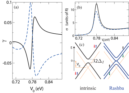
Figure 2: Skew scattering induced by SOC impurities close to a resonance in the cross section. (a) Skeweness $\gamma=\Sigma_{\perp}^{s}/\Sigma_{\parallel}^{s}$ as a function of $V_{0}$ for an intrinsic (Rashba)-type SOC scatterer [solid black line (dashed blue line)]. Even larger values of $\gamma$ are found near sharper resonances occurring at larger $V_{0}$ (not shown). (b) Transport cross section versus $V_{0}$. These panels have $R=4$ nm, $\hbar v_{F}k=0.1$ eV, and $\Delta=25$ meV. (c) Dispersion relation inside the SOC disk scatterer. Dashed orange lines are guidelines to the eye representing the bulk band structure of monolayer graphene.

As a measure of asymmetry in scattering events we adopt the so-called transport skewness; for intrinsic SOC scatterers, the latter is defined as $\gamma\equiv\Sigma_{\perp}^{s}/\Sigma_{\parallel}^{s}$, where $\Sigma_{\parallel}^{s}=\int d\theta(1-\cos\theta)\,|f_{\lambda}^{ss}(\theta)|^{2}$ is the transport cross section for a carrier with spin $s$ [for Rashba SOC see the discussion below Eq. (7)]. Exact evaluations show (i) $|\gamma|>0$ for local SOCs of the intrinsic type, (ii) local Rashba SOCs induce $|\gamma|>0$ provided that electron-hole symmetry is broken by an electrostatic term, i.e., $V_{0}\neq 0$, and (iii) $|\gamma|$ is maximum near resonances in $\Sigma_{\parallel}^{s}$. To illustrate these findings, we model the SOC active impurity as a uniform disk scatterer of radius $R$ (see Fig. 1), according to ${\cal V}_{\textrm{ad}}(r)=[V_{0}+\mathcal{V}_{\textrm{SO}}^{(I/R)}]\Theta(R-r)$, with $\Theta(.)$ denoting the Heaviside step function and $\mathcal{V}_{\textrm{SO}}^{(I/R)}$ being intrinsic or Rashba-type SOC with $\Delta_{I/R}(\mathbf{r})\equiv\Delta$. The different symmetries of these terms justifies studying them separately. Furthermore, it can be shown that interference between intrinsic and Rashba SOC does not suppress the resonant behavior of skewness (see SM). In our calculations we have taken $\Delta\sim 10$ meV, which is consistent with ab initio calculations for metal atoms adsorbed in graphene weeks11 ; Niu11 . The skewness of SOC active disk scatterers in the vicinity of a particular resonance is shown in Fig. 2. The function $\gamma(V_{0})$ follows an approximately asymmetric shape for both intrinsic and Rashba SOC. We further note that for Rashba-only SOC the skewness approaches zero as $V_{0}\rightarrow 0$ (not shown). We also found that $\gamma$ is larger near sharp resonances, typically occurring at large $V_{0}$. It is known that small doses of certain adatoms with large effective $V_{0}$ values produce resonances near the Fermi level of graphene Ferreira11 that might dominate charge transport (see Ref. [ExperimentsRS, ] for transport measurements in graphene covered with hydrogen). For dilute SOC disorder, the parameter $\gamma$ can therefore be seen as a figure of merit for the capability of generating net transverse spin currents via skew scattering. In fact, as shown in what follows, in the absence of other sources of impurities and at zero temperature, the spin Hall angle equals $\gamma$. Crucially, the results in Fig. 2 show that a large $V_{0}$ is not a necessary condition to obtain large skewness: although resonant impurities such as H induce giant effective potentials $V_{0}\sim 100$ eV (see Ref. [Ferreira11, ] and the references therein) and significant SOC via lattice distortion ahcn08 ; Gmitra13 ; Balakrishnan13 , clusters leading to $\mathcal{V}_{\textrm{SO}}$ of tens of mili-electron-volts most likely produce $V_{0}$ values below those found for chemisorbed adatoms. Large SOC active scatterers could be formed by the clustering of physisorbed transition metals inducing significant local enhancement of SOC, such as Au or In weeks11 ; Marchenko12 .

After analyzing the SHE due to a single scatterer, we next turn to the experimentally relevant situation of a dilute random ensemble of scatterers. We focus on the spin Hall current polarized out of the plane; see the SM for a discussion of in-plane polarization. Our goal is to compute the spin Hall angle defined as $\theta_{\textrm{sH}}=j_{\textrm{sH}}/j_{x}$, with $j_{x}=\sum_{s=\pm}\mathbf{j}_{s}\cdot\mathbf{e}_{x}$ and $j_{\textrm{sH}}=\sum_{s=\pm}s\mathbf{j}_{s}\cdot\mathbf{e}_{y}$ being the expectation values of the (charge) longitudinal and (spin) Hall currents, respectively. We safely neglect the quantum side-jump contribution to $j_{\textrm{sH}}$ which is subdominant with respect to skew scattering in the dilute regime of interest here Sinitsyn . Semiclassicaly, the current is computed according to $\mathbf{j}_{s}=-eg_{v}\sum_{\mathbf{k}}\delta n_{s}(\mathbf{k})\mathbf{v}_{\mathbf{k}}$, where $\mathbf{v}_{\mathbf{k}}=(1/\hbar)\nabla_{\mathbf{k}}\epsilon_{\mathbf{k}}$ is the band velocity and $\delta n_{s}(\mathbf{k})=n_{s}(\mathbf{k})-n^{0}(\mathbf{k})$ denotes the deviation of the spin-dependent distribution function from its equilibrium value $n^{0}(\mathbf{k})$ ($g_{v}=2$ is graphene’s valley degeneracy factor). To describe this situation, we need to solve the Boltzmann transport equation (BTE), which for the steady state in the presence of a uniform electric field $\boldsymbol{\boldsymbol{\mathcal{E}}}=\mathcal{E}\mathbf{e}_{x}$ reads as BTE_comment

$$\nabla_{\mathbf{k}}n_{s}(\mathbf{k})\cdot(-e\boldsymbol{\boldsymbol{\mathcal{E}}})=\sum_{\mathbf{p},s^{\prime}}\left[n_{s^{\prime}}(\mathbf{p})-n_{s}(\mathbf{k})\right]W_{s^{\prime}s}(\mathbf{p},\mathbf{k})\,,$$ (5)

where $W_{ss^{\prime}}(\mathbf{k},\mathbf{k}^{\prime})\propto|f^{ss^{\prime}}(\theta)|^{2}\>\delta(\epsilon_{\mathbf{k}}-\epsilon_{\mathbf{k}^{\prime}})$ with $\theta=\angle\left(\mathbf{k},\mathbf{k}^{\prime}\right)$ is the quantum-mechanical rate for processes with $\mathbf{k}\rightarrow\mathbf{\mathbf{k}^{\prime}}$ and $s\rightarrow s^{\prime}$. Notice that skew scattering implies that $W_{ss^{\prime}}(\mathbf{k},\mathbf{k}^{\prime})\neq W_{ss^{\prime}}(\mathbf{k}^{\prime},\mathbf{k})$; cf., Eq. (3). Here, $W_{ss^{\prime}}(\mathbf{k},\mathbf{k}^{\prime})\equiv\sum_{\alpha=1}^{R}W_{ss^{\prime}}^{(\alpha)}(\mathbf{k},\mathbf{k}^{\prime})$ takes into account all disorder sources, where $R\geq 1$ is the number of such sources. In linear response, the above BTE admits the following general solution

$$\delta n_{s}(\mathbf{k})=\nabla_{\mathbf{k}}n^{0}(\mathbf{k})\cdot\left[A_{s}(\mathbf{k})e\boldsymbol{\boldsymbol{\mathcal{E}}}+B_{s}(\mathbf{k})\left(\mathbf{\hat{z}}\times e\boldsymbol{\boldsymbol{\mathcal{E}}}\right)\right]\,,$$ (6)

where $n^{0}(\mathbf{k})$ is the Fermi-Dirac distribution. With these definitions, and at zero temperature, one finds $\theta_{\textrm{sH}}=B_{\uparrow}(k_{F})/A_{\uparrow}(k_{F})$, where $k_{F}$ is the Fermi momentum. The latter expression can be evaluated in closed form:

$$\left.\theta_{\textrm{sH}}\right|_{T=0}=\frac{\tau_{\parallel}^{*}(k_{F})}{\tau_{\perp}^{*}(k_{F})}=\bar{\gamma}\,,$$ (7)

where $\tau_{\parallel}^{*-1}=\sum_{s^{\prime},\mathbf{p}}\left(1-ss^{\prime}\cos\theta\right)W_{ss^{\prime}}(\mathbf{k},\mathbf{p})$ and $\tau_{\perp}^{*-1}=\sum_{s^{\prime},\mathbf{p}}ss^{\prime}\sin\theta\,W_{ss^{\prime}}(\mathbf{k},\mathbf{p})$. The spin Hall angle $\theta_{\textrm{sH}}$ equals the weighted skewness as defined by $\bar{\gamma}=\bar{\Sigma}_{\perp}^{*}/\bar{\Sigma}_{\parallel}^{*}$, where $\bar{\Sigma}_{\parallel(\perp)}^{*}\equiv\sum_{\alpha}\frac{n_{\alpha}}{n}\Sigma_{\parallel(\perp)\alpha}^{*}=(nv_{F}\tau_{\parallel(\perp)}^{*})^{-1}$ and $n=\sum_{\alpha}n_{\alpha}$ is the total areal density of impurities. The explicit solutions for $A_{s}(B_{s})$ further contain the familiar scattering times $\tau_{\parallel}$ and $\tau_{\perp}$ that do not enter in the ratio $B_{s}/A_{s}$. The spin-flip contribution to “star” rates differ from standard definitions, e.g., $\tau_{\parallel,\textrm{flip}}^{*-1}\sim\int d\theta\left(1+\cos\theta\right)W_{s\bar{s}}(\theta)\neq\tau_{\parallel,\textrm{flip}}^{-1}$. (For this reason, in the calculation of the skewness of a Rashba scatterer in Fig. 2 we have used $\Sigma_{\parallel}\rightarrow\Sigma_{\parallel}^{*}=\sum_{s^{\prime}}\int d\theta(1-ss^{\prime}\cos\theta)|f^{ss^{\prime}}(\theta)|^{2}$.) This fact has been largely unnoticed, which we believe is a consequence of inadequate treatments of the BTE; relaxation rates found here, on the other hand, result from the exact solution of linearized BTEs (see the SM for further details).

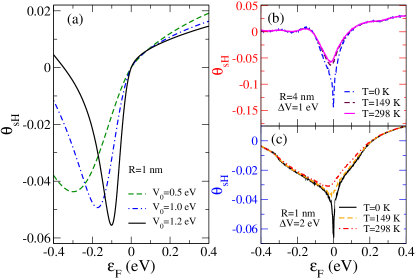
Figure 3: Spin Hall angle as a function of Fermi energy for a dilute random distribution of intrinsic SOC scatterers. (a) $\theta_{\textrm{sH}}$ at zero temperature for impurities producing a local electrostatic potential $V_{0}$. (b), (c) $\theta_{\textrm{sH}}$ at different temperatures and considering a random $V_{0}$ potential with uniform distribution $V_{0}\in[0,\Delta V]$. In all panels we have taken $\Delta_{I}=25$ meV.

A sizeable SHE is expected in relatively clean samples when cross sections for SOC active scatterers yield the dominant contribution to both transport and skew cross sections; Fig. 3 shows $\theta_{\textrm{sH}}$ [Eq. (7)] as a function of Fermi energy for pristine graphene decorated with a dilute concentration of intrinsic-type SOC scatterers ($\theta_{\textrm{sH}}$ induced by Rashba-type SOC is of the same order of magnitude and hence is not shown). The values obtained are comparable with those found in pure metals $|\theta_{\textrm{sH}}|\sim 0.01-0.1$ Morota11 ; Liu12 and are robust with respect to thermal fluctuations and disorder averaging [compare curves in Figs. 3(a) and 3(c)]; room temperature spin Hall angles of the order of $0.1$ are obtained for large scatterers with effective radius of just a few nanometers [see Fig. 3(b)]. Statistical distribution of scatterer sizes does not modify qualitatively this picture, indicating that large SOC active scatterers in clean graphene samples will drive the formation of robust spin Hall currents. Finally, we verified that time-reversal symmetry breaking by localized magnetic moments Lundeberg13 sitting at the impurities does not suppress the SHE (see the SM). Our findings suggest that functionalized graphene can be used to design spintronic integrated circuits with SHE-based spin-polarized current activation and control.

Acknowledgements. A.F., M.A.C. and A.H.C.N. acknowledge support from the National Research Foundation–Competitive Research Programme through the grant “Novel 2D materials with tailored properties: beyond graphene” (Grant No. R-144-000-295-281). T.G.R. acknowledges support from INCT–Nanocarbono, CNPq, and FAPERJ. M.A.C. acknowledges support from NSC and start-up funding from NTHU (Taiwan). Discussions with N.M.R. Peres and A. Pachoud are gratefully acknowledged.

Supplementary Material

I Analytical Solution of Boltzmann Transport Equations

In this section we solve analytically the Boltzmann transport equation (BTE). The low-energy Hamiltonian is given by $\mathcal{H}=\mathcal{H}_{0}+\mathcal{V}$, where $\mathcal{H}_{0}$ is the graphene-only term and $\mathcal{V}(\mathbf{r})=\sum_{i}\mathcal{V}^{(i)}(\mathbf{r}-\mathbf{r}_{i})$ is the disordered (spin-orbit) potential due to impurities located at random positions {$\mathbf{r}_{i}$}. Intervalley scattering is not considered in the present work and hence we drop any reference to the valley index. The BTE for a uniform graphene system reads as Ziman

$$\frac{\partial n_{\sigma}(\mathbf{k})}{\partial t}+\dot{\mathbf{k}}\cdot\nabla_{\mathbf{k}}n_{\sigma}(\mathbf{k}) =\;\mathcal{I}[n_{\sigma}(\mathbf{k})]\,.$$ (1)

In the above, $n_{\sigma}(\mathbf{k})$ is the carrier distribution function for carriers with momentum $\mathbf{k}$ and spin projection $\sigma$ along some axis and $\mathcal{I}[.]$ denotes the collision integral (see below). Under an external electric field $\boldsymbol{\boldsymbol{\mathcal{E}}}$, the BTE for carriers in the conduction (valence) band $\lambda=1$ ($\lambda=-1$) becomes

$$-e\lambda\boldsymbol{\boldsymbol{\mathcal{E}}}\cdot\mathbf{v}_{\mathbf{k}}^{(\lambda)}\left(\frac{\partial n^{0}}{\partial\epsilon}\right)_{\epsilon=\epsilon(\mathbf{k})}=\;\mathcal{I}[n_{\sigma}(\mathbf{k})]\,,$$ (2)

in first order in $\boldsymbol{\boldsymbol{\mathcal{E}}}$. Here, $\mathbf{v}_{\mathbf{k}}^{(\lambda)}=\lambda v_{F}(\cos\theta_{\mathbf{k}},\sin\theta_{\mathbf{k}}$) is the band velocity, $n^{0}=n^{0}(\epsilon)$ is the Fermi distribution function evaluated at energy $\epsilon$ and $-e<0$ is the electron charge. For simplicity we drop the band index in what follows. The collision integral for non-interacting charge carriers reads as

$$\mathcal{I}[n_{\sigma}(\mathbf{k})]=\sum_{\sigma^{\prime}=\sigma,\bar{\sigma}}\sum_{\mathbf{k}^{\prime}}\left[n_{\sigma^{\prime}}(\mathbf{k}^{\prime})-n_{\sigma}(\mathbf{k})\right]W_{\sigma^{\prime}\sigma}(\mathbf{k}^{\prime},\mathbf{k})\,,$$ (3)

where $W_{\sigma^{\prime}\sigma}(\mathbf{k}^{\prime},\mathbf{k})$ is the quantum-mechanical scattering probability for a process with $\mathbf{k}^{\prime}\rightarrow\mathbf{k}$ and $\sigma^{\prime}\rightarrow\sigma$ (here, $\bar{\sigma}\equiv-\sigma$). Note that under the stated conditions this quantity is the same in both valleys of graphene. For isotropic Fermi surfaces the distribution function solving Eq. (2) has the general form

$$n_{\sigma}(\mathbf{k})=n^{0}(k)+A_{\sigma}(k)|\mathbf{v}_{\mathbf{k}}|\cos[\phi(\mathbf{k})]+B_{\sigma}(k)|\mathbf{v}_{\mathbf{k}}|\sin[\phi(\mathbf{k})]\,,$$ (4)

where $k=|\mathbf{k}|$ and $\phi(\mathbf{x})$ denotes the angle that $\mathbf{v}_{\mathbf{x}}$ forms with the direction of $\boldsymbol{\boldsymbol{\mathcal{E}}}$. The functions $A_{\sigma}(k)$ and $B_{\sigma}(k)$ contain the information needed for the calculation of steady-state (spin-dependent) currents. Substitution of Eq. (4) into Eq. (2) yields the following system of equations

$$X(k) = \sum_{\sigma^{\prime}=\sigma,\bar{\sigma}}\left[A_{\sigma^{\prime}}\Gamma_{\sigma^{\prime}\sigma}^{\textrm{C}}-B_{\sigma^{\prime}}\Gamma_{\sigma^{\prime}\sigma}^{\textrm{S}}-A_{\sigma}\Gamma_{\sigma^{\prime}\sigma}^{\textrm{I}}\right]\,,$$ (5)

$$0 = \sum_{\sigma^{\prime}=\sigma,\bar{\sigma}}\left[B_{\sigma^{\prime}}\Gamma_{\sigma^{\prime}\sigma}^{\textrm{C}}+A_{\sigma^{\prime}}\Gamma_{\sigma^{\prime}\sigma}^{\textrm{S}}-B_{\sigma}\Gamma_{\sigma^{\prime}\sigma}^{\textrm{I}}\right]\,,$$ (6)

where $X(k)\equiv-e|\boldsymbol{\mathcal{E}}|\partial n^{0}/\partial\epsilon_{\mathbf{k}}$ and we have defined the relaxation rates:

$$\Gamma_{\sigma^{\prime}\sigma}^{\textrm{C}} = \int\frac{Sd^{2}\mathbf{k}^{\prime}}{(2\pi)^{2}}\cos\left[\phi(\mathbf{k})-\phi(\mathbf{k}^{\prime})\right]W_{\sigma^{\prime}\sigma}(\mathbf{k}^{\prime},\mathbf{k})\,,$$ (7)

$$\Gamma_{\sigma^{\prime}\sigma}^{\textrm{S}} = \int\frac{Sd^{2}\mathbf{k}^{\prime}}{(2\pi)^{2}}\sin\left[\phi(\mathbf{k})-\phi(\mathbf{k}^{\prime})\right]W_{\sigma^{\prime}\sigma}(\mathbf{k}^{\prime},\mathbf{k})\,,$$ (8)

$$\Gamma_{\sigma^{\prime}\sigma}^{\textrm{I}} = \int\frac{Sd^{2}\mathbf{k}^{\prime}}{(2\pi)^{2}}W_{\sigma^{\prime}\sigma}(\mathbf{k}^{\prime},\mathbf{k})\,,$$ (9)

where $S$ denotes the area of the system. For time-reversal invariant scattering, the relaxation rates obey $\Gamma_{\alpha\beta}^{X}=\varsigma\Gamma_{\bar{\alpha}\bar{\beta}}^{X}$ where $\varsigma=1$ ($\varsigma=-1$) for $X=I,C$ ($X=S$) symmetry . Using these relations, the solutions of (5)-(6) can be shown to acquire a particularly simple form in terms of four relaxation times:

$$A_{\sigma} = +A_{\bar{\sigma}}=-\frac{\tau_{\parallel}\tau_{\perp}\tau_{\perp}^{*}}{\tau_{\parallel}\tau_{\parallel}^{*}+\tau_{\perp}\tau_{\perp}}X\,,$$ (10)

$$B_{\sigma} = -B_{\bar{\sigma}}=-\frac{\tau_{\perp}\tau_{\parallel}\tau_{\parallel}^{*}}{\tau_{\parallel}\tau_{\parallel}^{*}+\tau_{\perp}\tau_{\perp}}X\,,$$ (11)

where

$$\frac{1}{\tau_{\parallel}} =\Gamma_{\sigma\sigma}^{\textrm{I}}-\Gamma_{\sigma\sigma}^{\textrm{C}}+\Gamma_{\sigma\bar{\sigma}}^{\textrm{I}}-\Gamma_{\sigma\bar{\sigma}}^{\textrm{C}}\,,$$ (12)

$$\frac{1}{\tau_{\parallel}^{*}} =\Gamma_{\sigma\sigma}^{\textrm{I}}-\Gamma_{\sigma\sigma}^{\textrm{C}}+\Gamma_{\sigma\bar{\sigma}}^{\textrm{I}}+\Gamma_{\sigma\bar{\sigma}}^{\textrm{C}}\,,$$ (13)

$$\frac{1}{\tau_{\perp}} =\Gamma_{\sigma\sigma}^{\textrm{S}}+\Gamma_{\sigma\bar{\sigma}}^{\textrm{S}}\,,\quad\frac{1}{\tau_{\perp}^{*}}=\Gamma_{\sigma\sigma}^{\textrm{S}}-\Gamma_{\sigma\bar{\sigma}}^{\textrm{S}}\,.$$ (14)

Here, $\tau_{\parallel}$ and $\tau_{\perp}$ are the standard transport and “skew” relaxation times Schliemann , whereas $\tau_{\parallel}^{*}$ and $\tau_{\perp}^{*}$ arise due to spin flips. Our study shows that a hierarchy of (non-equivalent) relaxation rates emerges when a quantum number such as spin is not conserved Lopes . This fact has been overlooked in previous approximate treatments of the BTE in similar systems Schliemann . Below we show that “star” relaxation times play a crucial role in the spin Hall effect.

For a driving electric field along the $x$ axis, the charge and spin Hall currents are defined as

$$j_{x}=-eg_{v}\int\frac{Sd^{2}\mathbf{k}^{\prime}}{(2\pi)^{2}}\left[n_{\sigma}(\mathbf{k})+n_{\bar{\sigma}}(\mathbf{k})\right]v_{\mathbf{k}}\cdot\mathbf{e}_{x}\,,$$ (15)

$$j_{\textrm{sH}}=-eg_{v}\int\frac{Sd^{2}\mathbf{k}^{\prime}}{(2\pi)^{2}}\left[n_{\sigma}(\mathbf{k})-n_{\bar{\sigma}}(\mathbf{k})\right]v_{\boldsymbol{k}}\cdot\mathbf{e}_{y}\,,$$ (16)

respectively, where $g_{v}=2$ is the valley degeneracy factor. At zero temperature $X\rightarrow-e|\boldsymbol{\mathcal{E}}|\delta(\epsilon_{\mathbf{k}}-\epsilon_{F})$ the integrals over $\mathbf{k}^{\prime}$ pick up only the contribution of states at the Fermi surface, and the spin Hall angle

$$\theta_{\textrm{sH}}\equiv\frac{j_{\textrm{sH}}}{j_{x}}\,$$ (17)

is totally determined by the star relaxation rates, i.e.,

$$\theta_{\textrm{sH}}=\frac{B_{\uparrow}-B_{\downarrow}}{A_{\uparrow}+A_{\downarrow}}=\frac{\tau_{\parallel}^{*}}{\tau_{\perp}^{*}}\,.$$ (18)

We note that the naive formula $\theta_{\textrm{sH}}=\tau_{\parallel}/\tau_{\perp}$ can only be correct in the absence of spin-flips, in which case $\tau_{\parallel(\perp)}^{*}=\tau_{\parallel(\perp)}$. When written in terms of cross sections, the physical interpretation of Eq. (18) becomes clear. Using $W_{\alpha\beta}(\mathbf{k},\mathbf{k}^{\prime})\propto\sigma_{\alpha\beta}(\theta)\delta(\epsilon_{\mathbf{k}}-\epsilon_{\mathbf{k}^{\prime}})$, where $\sigma_{\alpha\beta}(\theta)=|f^{\alpha\beta}(\theta)|^{2}$ is the impurity differential cross section at angle $\theta\equiv\phi(\mathbf{k}^{\prime})-\phi(\mathbf{k})$ ManyImp , we find

$$\theta_{\textrm{sH}}=\frac{\Sigma_{\perp}^{\text{*}}}{\Sigma_{\parallel}^{\text{*}}}\equiv\frac{\sum_{\sigma^{\prime}=\sigma,\bar{\sigma}}\int d\theta\>\sigma_{\sigma\sigma^{\prime}}(\theta)\,\sigma\sigma^{\prime}\sin\theta}{\sum_{\sigma^{\prime}=\sigma,\bar{\sigma}}\int d\theta\>\sigma_{\sigma\sigma^{\prime}}(\theta)\left(1+\sigma\sigma^{\prime}\cos\theta\right)}\,,$$ (19)

identifying $\theta_{\textrm{sH}}$ as a properly defined “skewness”, i.e., ratio of a skew cross section to a transport cross section.

II Calculation of Exact Scattering Amplitudes

II.1 Scatterers Producing Intrinsic-Type Spin-Orbit Coupling

In this section the partial-wave scattering amplitudes $\{S_{m}\}$ for disk scatterers endowed with spin-orbit coupling (SOC) of intrinsic type is derived. The components of the graphene spinor $\Psi^{\pm}(\mathbf{r})=(\psi_{A}^{\pm}({\mathbf{r}}),\psi_{B}^{\pm}({\mathbf{r}}))^{\textrm{T}}$ are decomposed in radial harmonics

$$\psi_{A}^{\pm}({\mathbf{r}})= \sum_{m=-\infty}^{\infty}g_{m,\pm}^{A}(r)e^{im\theta}\,,$$ (20)

$$\psi_{B}^{\pm}({\mathbf{r}})= \sum_{m=-\infty}^{\infty}g_{m,\pm}^{B}(r)e^{i(m+1)\theta}\,,$$ (21)

where $\theta\equiv\textrm{arg}(k_{x}+ik_{y})$, $\mathbf{k}$ is the wavevector, $m$ is the angular momentum quantum number, $\pm$ represents the spin projection and $A(B)$ are sublattice indices. The asymptotic form of the radial functions $g_{m,\pm}^{A}(r)$ and $g_{m,\pm}^{B}(r)$ determine the scattering amplitudes. The Hamiltonian is

$$\mathcal{H}=\mathcal{H}_{0}+\left(V_{0}+\Delta_{I}\tau_{z}\sigma_{z}s_{z}\right)\Theta(R-r)\,,$$ (22)

where $\mathcal{H}_{0}=v_{F}(\tau_{z}\sigma_{x}p_{x}+\sigma_{y}p_{y})$ is the low-energy free Hamiltonian and the second term is the disk scatterer potential. Here, $\Theta(.)$ is the Heaviside step function and $\boldsymbol{\mathbf{\sigma}},\mathbf{\boldsymbol{\tau}}$ and $\mathbf{s}$ are Pauli matrices for sublattice, valley and spin, respectively. We set $\hbar\equiv 1$ througout. The asymptotic form of waves at the $K$ valley ($\tau_{z}=1$) having spin projection $s=\mathbf{s}\cdot\mathbf{e}_{z}$ is

$$|\psi_{\lambda,\mathbf{k},s}({\bf r})\rangle =\left(\begin{array}[]{c}1\\ \lambda\end{array}\right)e^{ikr\cos(\theta)}|s\rangle+\frac{f^{ss}(\theta)}{\sqrt{-ir}}\left(\begin{array}[]{c}1\\ \lambda e^{i\theta_{{\bf k}}}\end{array}\right)e^{ikr}|s\rangle$$ (27)

$$+\frac{f^{s\bar{s}}(\theta)}{\sqrt{-ir}}\left(\begin{array}[]{c}1\\ \lambda e^{i\theta_{{\bf k}}}\end{array}\right)e^{ikr}|\bar{s}\rangle\ ,$$ (30)

where $\lambda=\pm 1$ denotes the carrier polarity, $\bar{s}=-s$ and $f^{ss}(\theta)$ and $f^{s\bar{s}}(\theta)$ are scattering amplitudes in the elastic and spin-flip channels, respectively. (For other choices of quantization axis see discussion in Sec. III.3.) Inside the disk of radius $R$, the dispersion relation satisfies $E-V_{0}=\lambda\sqrt{v_{F}^{2}k^{2}+\Delta_{I}^{2}}\equiv\epsilon$ and

$$|\psi_{\lambda,{\bf k},s}(\mathbf{r})\rangle=\left(\begin{array}[]{c}\sqrt{\epsilon+s\Delta_{I}}\\ \eta\sqrt{\epsilon-s\Delta_{I}}e^{i\theta_{{\bf k}}}\end{array}\right)e^{i{\bf{k}\cdot{\bf{r}}}}|s\rangle,$$ (31)

where $\eta=\mathrm{sgn}(\epsilon+|\Delta_{I}|)$. In order to identify the scattering amplitudes, we recast the wavefunction inside and outside the disk as a superposition of angular harmonics. For $r>R$, we have $E=\lambda v_{F}k$ and the partial-wave $m$ is given by

$$|\psi_{m}^{>}(r,\theta)\rangle =\left(\begin{array}[]{c}J_{m}(kr)e^{im\theta}\\ i\lambda J_{m+1}(kr)e^{i(m+1)\theta}\end{array}\right)|s\rangle$$ (34)

$$+S_{m}^{s}\left(\begin{array}[]{c}H_{m}^{(1)}(kr)e^{im\theta}\\ i\lambda H_{m+1}^{(1)}(kr)e^{i(m+1)\theta}\end{array}\right)|s\rangle,$$ (37)

whereas for $r<R$ one has

$$|\psi_{m}^{<}(r,\theta)\rangle=C_{m}\left(\begin{array}[]{c}\sqrt{\epsilon+s\Delta_{I}}J_{m}(\beta r)e^{im\theta}\\ i\eta\sqrt{\epsilon-s\Delta}J_{m+1}(\beta r)e^{i(m+1)\theta}\end{array}\right)|s\rangle,$$ (38)

with $\beta\equiv\sqrt{\epsilon^{2}-\Delta^{2}}/v_{F}$. The boundary condition $\psi_{m}^{>}(R,\theta)=\psi_{m}^{<}(R,\theta)$ gives rise to two equations fully determining the amplitudes $S_{m}^{s}$. Straighforward algebra yields

$$S_{m}^{s}=-\frac{\sqrt{\epsilon+s\Delta_{I}}J_{m+1}(kR)J_{m}(\beta R)-\frac{\eta}{\lambda}\sqrt{\epsilon-s\Delta_{I}}J_{m+1}(\beta R)J_{m}(kR)}{\sqrt{\epsilon+s\Delta_{I}}H_{m+1}^{(1)}(kR)J_{m}(\beta R)-\frac{\eta}{\lambda}\sqrt{\epsilon-s\Delta_{I}}J_{m+1}(\beta R)H_{m}^{(1)}(kR)}.$$ (39)

Naturally, in the absence of intervalley scattering $[\tau_{z},\mathcal{H}]=0$, calculations performed in the $K$ and $K^{\prime}$ valleys yield the same scattering amplitudes and hence the same transport quantities valleys .

II.2 Scatterers Producing Rashba-Type Spin-Orbit Coupling

If we consider a scatterer producing a Rashba-type SOC interaction in the form

$$\tilde{\mathcal{V}}=\left[V_{0}+\tau_{z}\Delta_{R}\left(\sigma_{x}s_{y}-\sigma_{y}s_{x}\right)\right]\Theta(R-r)\,,$$ (40)

the diagonalization of $\tilde{\mathcal{H}}=\mathcal{\tilde{\mathcal{H}}}_{0}+\tilde{\mathcal{V}}$ inside the disk ($r<R$) yields the spectrum $E-V_{0}=\xi\tau_{z}\Delta_{R}+\lambda\sqrt{v_{F}^{2}k^{2}+\Delta_{R}^{2}}=\epsilon_{\xi}(\mathbf{k})\equiv\epsilon_{\xi}$, where $\xi=\pm$ is the chirality of the band Hernando09_sup . For simplicity we restrict the subsequent analysis to carriers with positive polarity $\lambda=1$ and assume $|\epsilon|>2|\Delta_{R}|$. Eigenstates at the $K$ valley read as

$$|\psi_{\mathbf{k}}(\mathbf{r})\rangle=\left[\left(\begin{array}[]{c}1\\ \frac{\epsilon_{\xi}}{v_{F}k}e^{i\theta_{{\bf k}}}\end{array}\right)|\uparrow\;\rangle+i\xi\left(\begin{array}[]{c}\frac{\epsilon_{\xi}}{v_{F}k}e^{i\theta_{{\bf k}}}\\ e^{2i\theta_{{\bf k}}}\end{array}\right)|\downarrow\;\rangle\right]e^{i{\bf{k}\cdot{\bf{r}}}}.$$ (41)

Differently from the intrinsic SOC, Rashba-like interaction entangles spin and and pseudo-spin (sublattice), implying that spin-flips must be taken into account. As before, eigenstates inside and outside the disk scatterer can be recast into a superposition of angular harmonics. In the region $r>R$ we obtain

$$|\psi_{m}^{>}(r,\theta)\rangle =\left(\begin{array}[]{c}J_{m}(kr)e^{im\theta}\\ iJ_{m+1}(kr)e^{i(m+1)\theta}\end{array}\right)|\uparrow\;\rangle$$ (44)

$$+S_{m}^{\uparrow\uparrow}\left(\begin{array}[]{c}H_{m}^{(1)}(kr)e^{im\theta}\\ iH_{m+1}^{(1)}(kr)e^{i(m+1)\theta}\end{array}\right)|\uparrow\;\rangle$$ (47)

$$+S_{m+1}^{\uparrow\downarrow}\left(\begin{array}[]{c}H_{m+1}^{(1)}(kr)e^{i(m+1)\theta}\\ iH_{m+2}^{(1)}(kr)e^{i(m+2)\theta}\end{array}\right)|\downarrow\;\rangle.$$ (50)

In the above we assumed an incident wave with $s=1$. Inside the disk, the wave function regular at the origin is

$$|\psi_{m}^{<}(r,\theta)\rangle=\sum_{\xi}C_{\xi m} \left[\left(\begin{array}[]{c}J_{m}(\beta_{\xi}r)e^{im\theta}\\ i\frac{\epsilon_{\xi}}{v_{F}\beta_{\xi}}J_{m+1}(\beta_{\xi}r)e^{i(m+1)\theta}\end{array}\right)|\uparrow\;\rangle\right.$$ (53)

$$\left.+\xi\left(\begin{array}[]{c}\frac{\epsilon}{v_{F}\beta_{\xi}}J_{m+1}(\beta_{\xi}r)e^{i(m+1)\theta}\\ iJ_{m+2}(\beta_{\xi}r)e^{i(m+2)\theta}\end{array}\right)|\downarrow\;\rangle\right]\,,$$ (56)

where $\beta_{\xi}=\sqrt{\epsilon_{\xi}(\epsilon_{\xi}-2\xi\Delta_{R})}/v_{F}$. The matching conditions at $r=R$ yields four equations

$$J_{m}(kR)+S_{m}^{\uparrow\uparrow}H_{m}^{(1)}(kR) =\sum_{\xi}C_{\xi m}J_{m}(\beta_{\xi}R),$$ (57)

$$J_{m}(kR)+S_{m}^{\uparrow\uparrow}H_{m}^{(1)}(kR) =\sum_{\xi}C_{\xi m}J_{m}(\beta_{\xi}R),$$ (58)

$$S_{m}^{\uparrow\downarrow}H^{(1)}(kR) =\sum_{\xi}\xi\frac{\epsilon C_{\xi m}}{v_{F}\beta_{\xi}}J_{m+1}(\beta_{\xi}R),$$ (59)

$$S_{m}^{\uparrow\downarrow}H_{m+2}^{(1)}(kR) =\sum_{\xi}\xi C_{\xi m}J_{m+2}(\beta_{\xi}R).$$ (60)

Equations (57)–(60) can be shown to obey the required boundary conditions. Indeed, taking a superposition of partial waves $\psi=\sum_{m}i^{m}\psi_{m}$ the correct asymptotic limit for the Dirac equation in two dimensions is obtained, i.e.,

$$|\psi_{\mathbf{k}}(\mathbf{r})\rangle\rightarrow \left(\begin{array}[]{c}1\\ 1\end{array}\right)e^{ikr\cos\theta}|\uparrow\;\rangle+\sqrt{\frac{2}{i\pi kr}}\left(\begin{array}[]{c}1\\ e^{i\theta}\end{array}\right)e^{ikr}\times$$ (65)

$$\sum_{m=-\infty}^{\infty}e^{im\theta}\left[{S_{m}^{ss}}|\uparrow\;\rangle+{S_{m}^{s\bar{s}}}|\downarrow\;\rangle\right]\,.$$ (66)

The scattering amplitudes can be readily identified from the above expression:

$$f^{ss}(\theta) = \sqrt{\frac{2}{i\pi k}}\sum_{m=-\infty}^{\infty}{S_{m}^{ss}e^{im\theta}},$$ (67)

$$f^{s\bar{s}}(\theta) = \sqrt{\frac{2}{i\pi k}}\sum_{m=-\infty}^{\infty}{S_{m}^{s\bar{s}}e^{im\theta}}.$$ (68)

II.3 General Expressions of Cross Sections

The formulae given above allows determination of cross sections (or equivalently, relaxation rates) used in the BTE (Sec. I). For instance, the “star” transport and the “star” skew cross sections

$$\Sigma_{\parallel}^{*} =\sum_{s^{\prime}}\int d\theta(1-ss^{\prime}\cos\theta)|f^{ss^{\prime}}(\theta)|^{2}\,,$$ (69)

$$\Sigma_{\perp}^{*} =\sum_{s^{\prime}}\int d\theta\sin\theta ss^{\prime}|f^{ss^{\prime}}(\theta)|^{2}\,,$$ (70)

are conveniently written in terms of scattering amplitudes as

$$\Sigma_{\parallel}^{*} = \frac{4}{k}\sum_{s^{\prime}}\sum_{m=-\infty}^{\infty}\left\{|S_{m}^{ss^{\prime}}|^{2}-ss^{\prime}{\rm{Re}}[S_{m}^{ss^{\prime}}(S_{m+1}^{ss^{\prime}})^{*}]\right\}\,,$$ (71)

$$\Sigma_{\perp}^{*} = \frac{4}{k}\sum_{s^{\prime}}\sum_{m=-\infty}^{\infty}ss^{\prime}{\rm{Im}}[S_{m}^{ss^{\prime}}(S_{m+1}^{ss^{\prime}})^{*}].$$ (72)

These expressions together with the equations defining the scattering amplitudes explicitly [e.g., Eq. (39)] were used to create the plots of the skewness and spin Hall angle shown in the main text of the Letter.

III Additional Discussions

III.1 Time-Reversal Symmetry Breaking

In order to assess how time-reversal symmetry breaking potentially impacts on the spin Hall effect, it is enough to add a local exchange field $\mathcal{H}_{B}=\Delta_{B}s_{z}\Theta(R-r)$ to Eq. (22) and compute the spin Hall angle. Using the representation $\langle\mathbf{r}|\tilde{\Psi}\rangle$ referred to in Ref. valleys, , we obtain

$$\tilde{\mathcal{H}} =\tilde{\mathcal{H}}_{0}+\left(V_{0}+\Delta_{I}\sigma_{z}s_{z}+\Delta_{B}s_{z}\right)\Theta(R-r)\,.$$ (73)

The dispersion relation for $r<R$ satisfies $E-V_{0}-s\Delta_{B}=\tau_{z}\lambda\sqrt{\Delta_{I}^{2}+v_{F}^{2}k^{2}}\equiv\epsilon_{s}$. As in above, for simplicity we particularize our discussion to the conduction band $\lambda=1$. The eigenstates inside the disk read as .

$$|\psi_{m}^{<}(r,\theta)\rangle=C_{m}\left(\begin{array}[]{c}\sqrt{\epsilon_{s}+s\Delta_{I}}J_{m}(\beta_{s}r)e^{im\theta}\\ i\tau\zeta_{\tau}\sqrt{\epsilon_{s}-s\Delta_{I}}J_{m+1}(\beta_{s}r)e^{i(m+1)\theta}\end{array}\right)|s\rangle\,,$$ (74)

with $\tau\equiv\tau_{z}$, $\zeta_{\tau}=\textrm{sign}(\epsilon_{s}-|\Delta_{I}|)$ and $\beta_{s}=\sqrt{\epsilon_{s}^{2}-\Delta_{I}^{2}}/v_{F}$ Outside the disk we find

$$|\psi_{m}^{>}(r,\theta)\rangle =\left(\begin{array}[]{c}J_{m}(kr)e^{im\theta}\\ i\tau J_{m+1}(kr)e^{i(m+1)\theta}\end{array}\right)|s\rangle$$ (77)

$$+S_{m}^{s\tau}\left(\begin{array}[]{c}H_{m}^{(1)}(kr)e^{im\theta}\\ i\tau H_{m+1}^{(1)}(kr)e^{i(m+1)\theta}\end{array}\right)|s\rangle.$$ (80)

The skewness (or equivalently, the spin Hall angle at zero temperature) is given by

$$\gamma=\frac{B_{\uparrow}-B_{\downarrow}}{A_{\uparrow}+A_{\downarrow}}\,,$$ (81)

where $A_{\uparrow}\neq A_{\downarrow}$ and $B_{\uparrow}\neq-B_{\downarrow}$ for $\Delta_{B}\neq 0$. In the cases of interest the smallest energy scale will be the SOC (in the range 1–10 meV; see main text). We have verified that near resonances large $\gamma$ is obtained even in the strong exchange field limit $|\Delta_{B}|\gg|\Delta_{I}|$. This simple calculation illustrates that skew scattering is robust with respect to time-reversal symmetry breaking e.g., via local magnetic moments sitting at the SOC-active impurity sites.

III.2 Interference Between Intrinsic and Rashba-Type Spin-Orbit Couplings

We now briefly discuss the robustness of the spin Hall effect with respect to admixture of SOC terms. In realistic scenarios adsorbed species in graphene will give rise to local SOC terms with different symmetries, such as intrinsic and Rashba-type SOC.

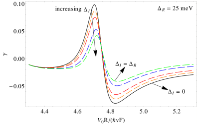
Figure 1: The skewness as function of the normalized eletrostatic potential for a disk scatterer producing an admixture of intrinsic and Rashba SOC. Values of intrinsic-type SOC are $\pm\{5,10,15,20,25\}$ meV [positive (negative) values are shown in left (right) panels]. Other parameters as in Fig. 2 in the manuscript.

We consider the following model:

$$\tilde{\mathcal{H}}=\tilde{\mathcal{H}}_{0}+\left[V_{0}+\Delta_{I}\sigma_{z}s_{z}+\Delta_{R}\tau_{z}(\sigma_{y}s_{x}-\sigma_{x}s_{y})\right]\Theta(R-r)\,.$$ (82)

Diagonalization inside the disk of radius $R$ yields

$$E-V_{0}+\xi\Delta_{R}+\lambda\sqrt{v_{F}^{2}k^{2}+\left(\Delta_{I}-\xi\Delta_{R}\right)^{2}}\equiv\epsilon_{\chi}(\mathbf{k})\equiv\epsilon\,.$$ (83)

The (non-normalized) eigenvectors in the $K$ valley (and for $\lambda=1$) can be written as

$$|\psi_{\xi}(\mathbf{r})\rangle=\left[\left(\begin{array}[]{c}e^{-i\theta_{\mathbf{k}}}\\ \frac{\epsilon_{\chi}(k)-\Delta_{I}}{v_{F}k}\end{array}\right)|\uparrow\;\rangle+i\xi\left(\begin{array}[]{c}\frac{\epsilon_{\chi}(k)-\Delta_{I}}{v_{F}k}\\ e^{i\theta_{\mathbf{k}}}\end{array}\right)|\downarrow\;\rangle\right]e^{i\mathbf{k}\cdot\mathbf{r}}\,.$$ (84)

Following the same procedure as outlined in the previous sections, we find the following set of equations:

$$J_{m}(kR)+S_{m}^{\uparrow\uparrow}H_{m}^{(1)}(kR) =\sum_{\xi}C_{\xi m}J_{m}(\beta_{\xi}R),$$ (85)

$$J_{m}(kR)+S_{m}^{\uparrow\uparrow}H_{m}^{(1)}(kR) =\sum_{\xi}C_{\xi m}J_{m}(\beta_{\xi}R),$$ (86)

$$S_{m}^{\uparrow\downarrow}H^{(1)}(kR) =\sum_{\xi}\xi\frac{\epsilon-\Delta_{I}}{v_{F}\beta_{\xi}}C_{\xi m}J_{m+1}(\beta_{\xi}R),$$ (87)

$$S_{m}^{\uparrow\downarrow}H_{m+2}^{(1)}(kR) =\sum_{\xi}\xi C_{\xi m}J_{m+2}(\beta_{\xi}R),$$ (88)

where $\beta_{\xi}=\sqrt{(\epsilon-\xi\Delta_{R})^{2}-(\Delta_{I}-\xi\Delta_{R})^{2}}$. The competition of intrinsic and Rashba couplings in the vicinity of a resonance is demonstrated in Fig. (1). We found that in general interference between SOC couplings do not supress the resonant enhancement of the skewness.

III.3 Quantization Axis: Arbitrary Direction of the Spin Polarization

In the main text of the Letter we have chosen to present our results with spin quantization axis along the $z$ direction. However, they can be easily generalized to any quantization direction. Physically, as we are dealing with unpolarized currents in the spin Hall effect, an arbitrary change in the quantization axis correspond to a measurement of the spin polarization in an arbitrary direction. The spin-dependent scattering amplitudes can be recast into matrix form:

$$\mathbf{F}=\left(\begin{array}[]{cc}f^{\uparrow\uparrow}(\theta)&f^{\uparrow\downarrow}(\theta)\\ f^{\downarrow\uparrow}(\theta)&f^{\downarrow\downarrow}(\theta)\end{array}\right).$$ (89)

Changing the spin quantization axis translates into a rotation in the spin space $\mathbf{F}^{\prime}=\mathbf{U}^{-1}\mathbf{F}\mathbf{U}.$ As an example, let us consider the calculation of the spin polarization in the $x$ direction. In this case, $\mathbf{U}$ is a $2\times 2$ Hadamard matrix, i.e.,

$$\mathbf{H}=\mathbf{H}^{-1}=\frac{1}{\sqrt{2}}\left(\begin{array}[]{cc}1&1\\ 1&-1\end{array}\right).$$ (90)

After performing the rotation, we find

$$\mathbf{F}_{x}=\frac{1}{2}\left(\begin{array}[]{cc}f^{\uparrow\uparrow}(\theta)+f^{\uparrow\downarrow}(\theta)+f^{\downarrow\uparrow}(\theta)+f^{\downarrow\downarrow}(\theta)&f^{\uparrow\uparrow}(\theta)+f^{\uparrow\downarrow}(\theta)-f^{\downarrow\uparrow}(\theta)-f^{\downarrow\downarrow}(\theta)\\ f^{\uparrow\uparrow}(\theta)-f^{\uparrow\downarrow}(\theta)+f^{\downarrow\uparrow}(\theta)-f^{\downarrow\downarrow}(\theta)&f^{\uparrow\uparrow}(\theta)-f^{\uparrow\downarrow}(\theta)-f^{\downarrow\uparrow}(\theta)+f^{\downarrow\downarrow}(\theta)\end{array}\right).$$ (91)

Moreover, using

$$f_{x}^{ss}(\theta) = \sqrt{\frac{2}{i\pi k}}\sum_{m=-\infty}^{\infty}{S_{m,x}^{ss}e^{im\theta}},$$ (92)

$$f_{x}^{s\bar{s}}(\theta) = \sqrt{\frac{2}{i\pi k}}\sum_{m=-\infty}^{\infty}{S_{m,x}^{s\bar{s}}e^{im\theta}},$$ (93)

the new amplitudes $S_{m,x}^{ss^{\prime}}$ can be written in terms of the amplitudes that were calculated in the previous sections. As a result, the “star” cross sections in the new quantization axis can be obtained by using the relations given by equations 71 and 72. Our calculations show that $\Delta_{I}$-scatterers give rise to zero skewness for carriers spin-polarized along $x$. On the other hand, $\Delta_{R}$-scatterers produces skew-scattering cross sections of the same order of magnitude than those for carriers spin-polarized along $z$. Physically, it means is that in order to measure the spin Hall effect produced by intrinsic-type SOC, it is necessary to detect the spin-polarization in the $z$ direction while a measurement of the spin-polarization in $x$ only detects the spin Hall effect due to Rashba.

IV Limitations of Perturbative Approaches: The Distorted-Wave Born Approximation

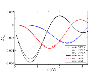
Figure 2: Comparison between the exact value of $\Delta\delta_{m}=\delta_{V_{0}+\textrm{SO}}-\delta_{V_{0}}$ and the DWBA result. The parameters used in this plot are: $\Delta_{I}s_{z}=7$ eV, $V_{0}=70$ meV and $R=1$ nm.

In this section, we provide a few examples of the limitations of the distorted-wave Born approximation (DWBA) when applied to study spin Hall effect (SHE) in graphene. We first derive the DWBA for a general class of potentials of the form

$$\mathcal{V}_{a}=V_{a}(r)+W_{a}(r)\sigma_{z}\,,$$ (94)

where $W_{a}(r)$ denotes the sublattice symmetry breaking term. In analogy to the derivation for a scalar potential in the Schrödinger equation Ballantine_sup , it is necessary to write two copies of the Dirac equation corresponding to different potentials, $V_{1}$ and $V_{2}$. The scattering amplitudes (or phase-shifts, $\delta_{m}^{[1]}$) of the simpler problem $\mathcal{H}_{1}\equiv\mathcal{H}_{0}+\mathcal{V}_{1}$ are assumed to be known. Let us denote the eigenstates of $\mathcal{H}_{a}\equiv\mathcal{H}_{0}+V_{a}$ in a given valley by

$$\Psi_{m}^{a}(r,\phi)=e^{im\phi}\left(\begin{array}[]{c}F_{a}(r)\\ G_{a}(r)e^{i\phi}\end{array}\right),$$ (95)

and $a=1,2$. We aim at finding the phase-shifts induced by the sublattice breaking term $W(r)$. Inserting the ansatz (95) into the Dirac equation, and using the asymptotic form of graphene wavefunctions

$$\Psi_{m}^{a}(r,\phi) \rightarrow \sqrt{\frac{2}{\pi kr}}\left[\begin{array}[]{c}\cos\left(kr-\varphi_{m}+\delta_{m}^{a}\right)\\ \lambda i\sin\left(kr-\varphi_{m}+\delta_{m}^{a}\right)\end{array}\right]\,,$$ (98)

where $\varphi_{m}=(2m+1)\pi/4$, we find

$$\frac{2\lambda}{\pi k}\sin\left(\delta_{m}^{[1]}-\delta_{m}^{[2]}\right) =\int_{0}^{\infty}drr\left[\frac{\delta\mathcal{V}_{+}}{\hbar v_{F}}F_{1}(r)F_{2}(r)\right.$$

$$\left.-\frac{\delta\mathcal{V}_{-}}{\hbar v_{F}}G_{1}(r)G_{2}(r)\right]\,,$$ (99)

where $\delta\mathcal{V}_{\pm}\equiv V_{2}\pm W_{2}-(V_{1}\pm W_{1})$. The above result is still exact; the DWBA is derived by employing the “Born approximation”: $F_{2}(r)\simeq F_{1}(r)$ and $G_{2}(r)\simeq G_{1}(r)$. Specializing to the case of interest, i.e., $V_{1}=V_{2}=V_{0}(r)$, $W_{1}=0$, and $W_{2}=W(r)$, the DWBA yields

$$\Delta\delta_{m}=-\frac{\zeta\pi k}{2\hbar v_{F}}\int_{0}^{\infty}drrW(r)\left[f_{m}(r)^{2}+g_{m}(r)^{2}\right],$$ (100)

where $\Delta\delta_{m}=\delta_{m}^{[2]}-\delta_{m}^{[1]}$ is the correction to the $m$-th phase-shift $\delta_{m}^{[1]}$ introduced by the sublattice breaking term $W(r)$. In the above, $f_{m}(g_{m})$ are the partial-wave amplitudes of the simpler problem $\mathcal{H}_{1}=\mathcal{H}_{0}+V_{0}(r)$ and $\zeta=\mathrm{sgn}(E-V_{0})$. We can use the equation above to calculate $\Delta\delta_{m}$ explicitly for an intrinsic-type disk scatterer with $V_{0}(r)=V_{0}\Theta(R-r)$ and $W(r)=\Delta_{I}s_{z}\Theta(R-r)$. We find

$$\Delta\delta_{m}=-\frac{\zeta\pi s_{z}}{2}\frac{\Delta_{I}k}{\hbar v_{F}\alpha^{2}}\int_{0}^{\alpha R}duu\left[J_{m}(u)^{2}-J_{m+1}(u)^{2}\right].$$ (101)

where $\alpha\equiv|k-V_{0}/{\hbar v_{F}}|$. The above expression can be further simplified using the properties of Bessel functions (not shown). In Fig. 2 we can see the comparison between this approximation and the exact result using Eq. (39) and the relation $S_{m}^{s}=ie^{i\delta_{m}^{s}}\sin(\delta_{m}^{s})$. The skew cross section can be easily calculated under the DWBA:

$$\Sigma_{\perp}^{\textrm{DWBA}}=\frac{2}{k}\sum_{m=-\infty}^{\infty}(\Delta\delta_{m}-\Delta\delta_{m+1})\cos[2(\delta_{m}^{[1]}-\delta_{m+1}^{[1]})].$$ (102)

The DWBA seems promising to compute phase-shifts for intrinsic-type scatterers in the presence of a scalar potential. However, it fails to correctly describe the skew cross section (and thus SHE) for other symmetries or in the presence of resonant scattering. Here, we briefly discuss a few situations where the approximation is not valid. Our first example is provided by a void in graphene, which is described by the boundary condition requiring that the A-sublattice component of the spinor $|\psi_{\mathbf{k}}(\mathbf{r})\rangle$ vanishes at $r=R$. Hence, the spin-independent part of the scattering phase shift $\delta_{m}^{[1]}$ fullfils:

$$\tan\delta_{m}^{[1]}=\frac{J_{m}(kR)}{Y_{m}(kR)}.$$ (103)

Note the symmetry $\delta_{-m}^{[1]}=\delta_{m}^{[1]}$. If we assume that the intrinsic-type potential only acts in the edge of the void, i.e., $W(r)=R\Delta_{I}\delta(r-R)\tau_{z}\sigma_{z}s_{z}$, then, the DWBA gives

$$\Delta\delta_{m} \propto\int rdr\>\Psi_{m}^{{\dagger}}(r,\phi)W(r)\Psi_{m}(r,\phi)$$

$$=R\Delta_{I}\frac{\left[Y_{m}(kR)J_{m+1}(kR)-Y_{m+1}(kR)J_{m}(kR)\right]^{2}}{Y_{m}^{2}(kR)}$$

$$\propto\Delta_{I}\,,$$ (104)

where we have used the Wronskian identity for Bessel function, which implies that $Y_{m}(x)J_{m+1}(x)-Y_{m+1}(x)J_{m}(x)=2/(\pi x)$. Hence, within the DWBA, $\delta_{m}^{[2]}=\delta_{-m}^{[2]}$, that is, the same symmetry as for the void potential, which implies the absence of skew scattering and therefore SHE.

A second example is provided by a generic Rashba-type scatterer, for which $W(r)=\Delta_{R}(r)\left(\tau^{z}\sigma^{x}s^{y}-\sigma^{y}s^{x}\right)$. It can be shown that within the DWBA, and at the lowest order in $\Delta_{R}$, only the spin-flip amplitude $f^{s\bar{s}}(\theta)\neq 0$ gets corrected and therefore the skew cross section for $z$-polarization (and hence SHE) is zero in this approximation, just as in the previous example.

References

• (1) M. I. Dyakonov and V. I. Perel, JETP Lett. 13, 467 (1971).
• (2) J. E. Hirsch, Phys. Rev. Lett. 83, 1834 (1999).
• (3) S. Zhang, Phys. Rev. Lett. 85, 393 (2000).
• (4) T. Jungwirth, J. Wunderlich, and K. Olejnik, Nat. Mater. 11, 382 (2012).
• (5) Y. K. Kato, R. C. Myers, A. C. Gossard, and D. D. Awschalom, Science 306, 1910 (2004).
• (6) V. Sih, R. C. Myers, Y. K. Kato, W. H. Lau, A. C. Gossard, and D. D. Awschalom, Nat. Phys. 1, 31 (2005).
• (7) K. Ando and E. Saitoh, Nat. Commun. 3, 629 (2012).
• (8) S. O. Valenzuela, and M. Tinkham, Nature (London) 442, 176 (2006).
• (9) T. Seki, Y. Hasegawa, S. Mitani, S. Takahashi, H. Imamura, S. Maekawa, J. Nitta, and K. Takanashi, Nature Mater. 7, 125 (2008).
• (10) L. Liu, T. Moriyama, D. C. Ralph, and R. A. Buhrman, Phys. Rev. Lett. 106, 036601 (2011).
• (11) L. Liu, C.-F. Pai, Y. Li, H. W. Tseng, D. C. Ralph, and R. A. Buhrman1, Science 336, 555 (2012).
• (12) M. Morota, Y. Niimi, K. Ohnishi, D. H. Wei, T. Tanaka, H. Kontani, T. Kimura and Y. Otani, Phys. Rev. B 83, 174405 (2011).
• (13) K. S. Novoselov, A. K. Geim, S. V. Morozov, D. Jiang, M. I. Katsnelson, I. V. Grigorieva, S. V. Dubonos, and A. A. Firsov, Nature (London) 438, 197 (2005); Y. Zhang, Y.-W. Tan, H. L. Stormer, and P. Kim, Nature (London) 438, 201 (2005); A. H. Castro Neto, F. Guinea, N. M. R. Peres, K. S. Novoselov, and A. K. Geim, Rev. Mod. Phys. 81, 109 (2009).
• (14) N. Tombros, C. Jozsa, M. Popinciuc, H. T. Jonkman, and B. J. van Wees, Nature (London) 448, 571 (2007).
• (15) S. Cho, Y. F. Chen, and M. S. Fuhrer, Appl. Phys. Lett. 91, 123105 (2007).
• (16) W. Han, K. Pi, K. M. McCreary, Y. Li, J. J. I. Wong, A. G. Swartz, and R. K. Kawakami, Phys. Rev. Lett. 105, 167202 (2010).
• (17) A. Avsar, T.-Y. Yang, S. Bae, J. Balakrishnan, F. Volmer, M. Jaiswal, Z. Yi, S. R. Ali, G. Güntherodt, B. H. Hong, B. Beschoten, and B. Özyilmaz, Nano Lett. 11 2363 (2011).
• (18) B. Dlubak, M.-B. Martin, C. Deranlot, B. Servet, S. Xavier, R. Mattana, M. Sprinkle, C. Berger, W. A. De Heer, F. Petroff, A. Anane, P. Seneor, and A. Fert, Nat. Phys. 8, 557 (2012).
• (19) D. Huertas-Hernando, F. Guinea, and A. Brataas, Phys. Rev. B 74, 155426 (2006).
• (20) S. Konschuh, M. Gmitra, and J. Fabian, Phys. Rev. B 82, 245412 (2010).
• (21) D. Pesin and A. H. MacDonald, Nat. Mater. 11, 409 (2012).
• (22) D. Marchenko, A. Varykhalov, M. R. Scholz, G. Bihlmayer, E. I. Rashba, A. Rybkin, A. M. Shikin, and O. Rader. Nat. Commun. 3, 1232 (2012).
• (23) A. H. Castro Neto and F. Guinea, Phys. Rev. Lett. 103, 026804 (2009).
• (24) C. Weeks, J. Hu, J. Alicea, M. Franz, and R. Wu, Phys. Rev. X 1, 021001 (2011).
• (25) V. K. Dugaev, M. Inglot, E. Y. Sherman, and J. Barnaś, Phys. Rev. B 82, 121310(R) (2010); A. Dyrdał, and J. Barnaś, Phys. Rev. B 86, 161401(R) (2012).
• (26) C. L. Kane and E. J. Mele, Phys. Rev. Lett. 95, 226801 (2005).
• (27) V. V. Mkhitaryan, and M. E. Raikh, Phys. Rev. B 77, 245428 (2008).
• (28) A. C. Hewson, The Kondo Problem to Heavy Fermions (Cambridge University Press, Cambridge, England, 1993).
• (29) G.-Y. Guo, S. Maekawa, and N. Nagaosa, Phys. Rev. Lett. 102, 036401 (2009).
• (30) T. Stauber, N. M. R. Peres, and F. Guinea, Phys. Rev. B 76, 205423 (2007); J. P. Robinson, H. Schomerus, L. Oroszlany, and V. I. Fal’ko, Phys. Rev. Lett. 101, 196803 (2008). T. O. Wehling, S. Yuan, A. I. Lichtenstein, A. K. Geim, M. I. Katsnelson, Phys. Rev. Lett. 105, 056802 (2010)
• (31) A. Ferreira, J. Viana-Gomes, J. Nilsson, E. R. Mucciolo, N. M. R. Peres, and A. H. Castro Neto, Phys. Rev. B 83, 165402 (2011).
• (32) J. Balakrishnan, G. K. W. Koon, M. Jaiswal, A. H. Castro Neto, and B. Özyilmaz, Nat. Phys. 9, 284 (2013).
• (33) L. E. Ballantine. Quantum Mechanics: A Modern Development (World Scientific, Singapore, 1998).
• (34) T. G. Rappoport, B. Uchoa, and A. H. Castro Neto, Phys. Rev. B 80, 245408 (2009).
• (35) K. Pi, Wei Han, K. M. McCreary, A. G. Swartz, Yan Li, and R. K. Kawakami, Phys. Rev. Lett. 104, 187201 (2010).
• (36) M. Gmitra, D. Kochan, and J. Fabian. Phys. Rev. Lett. 110, 246602 (2013).
• (37) J. Ding, Z. Qiao, W. Feng, Y.Yao, and Q. Niu, Phys. Rev. B 84, 195444 (2011).
• (38) J. Katoch, J.-H. Chen, R. Tsuchikawa, C. W. Smith, E. R. Mucciolo, and M. Ishigami, Phys. Rev. B 82, 081417(R) (2010). Z. H. Ni, L. A. Ponomarenko, R. R. Nair, R. Yang, S. Anissimova, I. V. Grigorieva, F. Schedin, Z. X. Shen, E. H. Hill, K. S. Novoselov, and A. K. Geim, Nano Lett. 10, 3868 (2010).
• (39) N. A. Sinitsyn, J. Phys. Condens. Matter 20, 023201 (2008).
• (40) We have neglected spin coherence in $n_{s}(\mathbf{k})$, keeping only diagonal terms, which is expected to be a good approximation at room temperature. We further note that the BTE does not describe transport close to the Dirac point.
• (41) M. B. Lundeberg, R. Yang, J. Renard, and J. A. Folk, Phys. Rev. Lett. 110, 156601 (2013).

References

• (1) J. M. Ziman, Principles of the Theory of Solids, 2nd ed. (Cambridge University Press, Cambridge, England, 1979).
• (2) These relations can be easily shown invoking $W_{\sigma\sigma^{\prime}}(\mathbf{k},\mathbf{k}^{\prime})=|T_{\sigma^{\prime}\sigma}(\mathbf{k}^{\prime},\mathbf{k})|^{2}$ and exploiting the symmetries of the $T$ matrix; see Eq. (3) in the main text of the Letter and comments therein.
• (3) J. Schliemann and D. Loss, Phys. Rev. B 68, 165311 (2003).
• (4) Multiple scattering rates in rigorous treatments of the BTE have been found in the context of granular systems; see J. Viana Lopes, J. M. B. Lopes dos Santos, and Y. G. Pogorelov, Phys. Rev. B 66, 064416 (2002).
• (5) When multiple disorder sources are present, weighted summations are taken in the usual way: $W_{\alpha\beta}(\mathbf{k},\mathbf{\mathbf{k}^{\prime}})=\sum_{j}W_{\alpha\beta}^{j}(\mathbf{k},\mathbf{k}^{\prime})\propto\sum_{j}n^{(j)}\sigma_{\alpha\beta}^{j}(\theta)\delta(\epsilon_{\mathbf{k}}-\epsilon_{\mathbf{k}^{\prime}})$ with $n^{(j)}$ being the areal density of impurities of type $j$.
• (6) In fact, using the representation $|\tilde{\Psi}\rangle=(\psi_{A}^{K},\psi_{B}^{K},\psi_{B}^{K^{\prime}},\psi_{A}^{K^{\prime}})^{\textrm{T}}\otimes|s\rangle$ yields an effective $\mathcal{H}$ in the form of two copies of the Dirac Hamiltonian $\tilde{\mathcal{H}}_{0}=v_{F}\tau_{z}\boldsymbol{\sigma}\cdot\mathbf{p}$ plus an interaction term with the same form in both valleys, i.e., $\tilde{\mathcal{V}}=\left(V_{0}+\Delta_{I}\sigma_{z}s_{z}\right)\Theta(R-r)$, implying that gauge-invariant quantities, such as the polarization and the conductivity, are insensitive to the choice of valley. Similar arguments can be used in the case of Rashba-type scatterers or for any type of SOC conserving the valley index.
• (7) D. Huertas-Hernando, F. Guinea, and A. Brataas, Phys. Rev. Lett. 103, 146801 (2009).
• (8) L. E. Ballantine. Quantum Mechanics: A Modern Development (World Scientific, Singapore, 1998).