A New Analysis of the DS-CDMA
Cellular Uplink Under Spatial Constraints

Abstract

A new analysis is presented for the direct-sequence code-division multiple access (DS-CDMA) cellular uplink. For a given network topology, closed-form expressions are found for the outage probability and rate of each uplink in the presence of path-dependent Nakagami fading and log-normal shadowing. The topology may be arbitrary or modeled by a random spatial distribution for a fixed number of base stations and mobiles placed over a finite area with the separations among them constrained to exceed a minimum distance. The analysis is more detailed and accurate than existing ones and facilitates the resolution of network design issues, including the influence of the minimum base-station separation, the role of the spreading factor, and the impact of various power-control and rate-control policies. It is shown that once power control is established, the rate can be allocated according to a fixed-rate or variable-rate policy with the objective of either meeting an outage constraint or maximizing throughput. An advantage of the variable-rate policy is that it allows an outage constraint to be enforced on every uplink, whereas the fixed-rate policy can only meet an average outage constraint.

I Introduction

The classical analysis of the uplinks $\left(\text{e.g., \cite[cite]{[\@@bibref{}{gil}{}{}]}},\text{ \cite[cite]{[\@@bibref{}{vit}{}{}]}, \cite[cite]{[\@@bibref{}{zor}{}{}]}}\right)$ in a cellular network entails a number of questionable assumptions. Among the principal ones are the existence of a lattice or regular grid of base stations and the modeling of intercell interference at a base station as a fixed fraction of the total interference. Although conceptually simple and locally tractable, the grid assumption is a poor model for actual base-station deployments, which cannot assume a regular grid structure due to a variety of regulatory and physical constraints. The intercell-interference assumption is untenable because the fractional proportion of intercell interference varies substantially with the mobile and base-station locations, the shadowing, and the fading.

More recent analyses of cellular networks (e.g., [4], [5]) locate the mobiles and/or base stations according to a two-dimensional Poisson point process (PPP) over a network that extends infinitely on the Euclidian plane, thereby allowing the use of analytical tools from stochastic geometry [6], [7]. Although the two principal limitations of the classical approach are eliminated, the PPP approach is still unrealistic because it cannot model networks of finite area and does not permit a minimum separation between base stations or between mobiles, although both minimum separations are characteristic of actual macro-cellular deployments.

The analysis in this paper is driven by a new closed-form expression [8] for the conditional outage probability of a communication link, where the conditioning is with respect to an arbitrary realization of the network topology. The approach involves drawing realizations of the network according to the desired spatial and shadowing models, and then computing the outage probability. Because the outage probability is averaged over the fading, it can be found in closed form with no need to simulate the corresponding channels. A Nakagami-m fading model is assumed, which models a wide class of channels, and the fading parameters do not need to be identical for all communication links. This flexibility allows the modeling of distance-dependent fading, where mobiles close to the base station have a dominant line-of-sight (LOS) path, while the more distant mobiles are non-LOS. The analysis can characterize more than just the average performance of a typical uplink. The outage probability of each uplink can be constrained, and the statistics of the rate provided to each mobile for its uplink can be determined under various power-control and rate-control policies.

Although our analysis is applicable for arbitrary topologies, we focus on a constrained random spatial approach to model the direct-sequence code-division multiple access (DS-CDMA) uplink. The spatial model places a fixed number of base stations within a region of finite extent. The model enforces a minimum separation among the base stations for each network realization, which comprises a base-station placement, a mobile placement, and a shadowing realization. The model for both mobile and base-station placement is a binomial point process (BPP) with repulsion, which we call a uniform clustering model [8].

A DS-CDMA uplink differs from a downlink, which has been presented in a separate paper [9], in at least four significant ways. First, the sources of interference are many mobiles for the uplink whereas the sources are a few base stations for the downlink. Second, sectorization is a critical factor in uplink performance whereas it is of minor importance in downlink performance. Third, the uplink signals arriving at a base station are asynchronous and, hence, non-orthogonal. Fourth, base stations are equipped with better transmit high-power amplifiers and receive low-noise amplifiers than the mobiles. The net result is that the operational signal-to-noise ratio is typically 5 - 10 dB lower for the uplink than for the downlink.

II Network Model

Cells may be divided into sectors by using several directional sector antennas or arrays, each covering disjoint angular sectors, at the base stations. Only mobiles in the directions covered by a sector antenna can cause multiple-access interference on the uplink from a mobile to its associated sector antenna. Thus, the number of interfering signals on an uplink is reduced approximately by a factor equal to the number of sectors. Practical sector antennas have patterns with sidelobes that extend into adjacent sectors, but the performance degradation due to overlapping sectors is significant only for a small percentage of mobile locations. Three ideal sector antennas and sectors per base station, each covering $2\pi/3$ radians, are assumed in the subsequent analysis. The mobile antennas are assumed to be omnidirectional.

The network comprises $C$ base stations and cells, $3C$ sectors $\{S_{1},...,S_{3C}\},$ and $M$ mobiles $\{X_{1},...,X_{M}\}$. The base stations and mobiles are confined to a finite area, which is assumed to be a circle of radius $r_{\mathsf{net}}$ and area $\pi r_{\mathsf{net}}^{2}$. The sector boundary angles are the same for all base stations. The variable $S_{j}$ represents both the $j^{th}$ sector antenna and its location, and $X_{i}$ represents the $i^{th}$ mobile and its location. An exclusion zone of radius $r_{\mathsf{bs}}$ surrounds each base station, and no other base stations or mobiles are allowed within this zone. Similarly, an exclusion zone of radius $r_{\mathsf{m}}$ surrounds each mobile where no other mobiles are allowed.

Example network topologies are shown in Fig. 1. The left subfigure shows the locations of actual base stations in a small city with hilly terrain. The base-station locations are given by the large filled circles, and the Voronoi cells are indicated in the figure. The minimum base-station separation is observed to be about 0.43 km. The right subfigure shows a portion of a randomly generated network with average number of mobiles per cell $M/C=16$, a base-station exclusion radius $r_{\mathsf{bs}}=0.25$, and a mobile exclusion radius $r_{\mathsf{m}}=0.01$. The locations of the mobiles are represented by small dots, and light lines indicate the angular coverage of sector antennas.

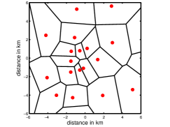
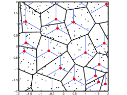
Figure 1: Example network topologies. Base stations are represented by large red circles, and cell boundaries are represented by solid black lines. Left subfigure: Actual base station locations from a current cellular deployment. Right subfigure: Simulated base-station locations using a base-station exclusion zone $r_{\mathsf{bs}}=0.25$. In the right subfigure, the simulated positions of the mobiles are represented by black dots, the sector boundaries are represented by light blue lines, and the average cell load is $M/C=16$ mobiles.

Consider a reference receiver of a sector antenna that receives a desired signal from a reference mobile within its cell and sector. Both intracell and intercell interference are received from other mobiles within the covered angle of the sector, but interference from mobiles in extraneous sectors is negligible. Duplexing is assumed to prevent interference from other sector antennas. The varying propagation delays from the interfering mobiles cause their interference signals to be asynchronous with respect to the desired signal.

In a DS-CDMA network of asynchronous quadriphase direct-sequence systems, a multiple-access interference signal with power $I$ before despreading is reduced after despreading to the power level $Ih(\tau_{o})/G$, where G is the processing gain or spreading factor, and $h(\tau_{o})$ is a function of the chip waveform and the timing offset $\tau_{o}$ of the interference spreading sequence relative to that of the desired or reference signal. If $\tau_{o}$ is assumed to have a uniform distribution over [0, $T_{c}],$ then the expected value of $h(\tau_{o})$ is the chip factor $h$ . For rectangular chip waveforms, $h=2/3$ [10], [11]. It is assumed henceforth that $G/h(\tau_{o})$ is a constant equal to $G/h$ at each sector receiver in the network.

Let $\mathcal{A}_{j}$ denote the set of mobiles covered by sector antenna $S_{j}$. A mobile $X_{i}\in\mathcal{A}_{j}$ will be associated with $S_{j}$ if the mobile’s signal is received at $S_{j}$ with a higher average power than at any other sector antenna in the network. Let ${\mathcal{X}}_{j}\subset\mathcal{A}_{j}$ denote the set of mobiles associated with sector antenna $S_{j}$. Let $X_{r}\in\mathcal{X}_{j}$ denote a reference mobile that transmits a desired signal to $S_{j}$. The power of $X_{r}$ received at $S_{j}$ is not significantly affected by the spreading factor and depends on the fading and path-loss models. The power of $X_{i},$ $i\neq r,$ received at $S_{j}$ is nonzero only if $X_{i}\in\mathcal{A}_{j},$ is reduced by $G/h,$ and also depends on the fading and path-loss models. We assume that path loss has a power-law dependence on distance and is perturbed by shadowing. When accounting for fading and path loss, the despread instantaneous power of $X_{i}$ received at $S_{j}$ is

$$\rho_{i,j}=\begin{cases}{P}_{r}g_{r,j}10^{\xi_{r,j}/10}f\left(||S_{j}-X_{r}||\right)&i=r\\ \left(\frac{h}{G}\right){P}_{i}g_{i,j}10^{\xi_{i,j}/10}f\left(||S_{j}-X_{i}||\right)&i:X_{i}\in\mathcal{A}_{j}\backslash X_{r}\\ 0&i:X_{i}\notin\mathcal{A}_{j}\end{cases}$$ (1)

where $g_{i,j}$ is the power gain due to fading, $\xi_{i,j}$ is a shadowing factor, ${P}_{i}$ is the power transmitted by $X_{i}$, and $\mathcal{A}_{j}\backslash X_{r}$ is set $\mathcal{A}_{j}$ with element $X_{r}$ removed (required since $X_{r}$ does not interfere with itself). The {$g_{i,j}\}$ are independent with unit-mean, and $g_{i,j}=a_{i,j}^{2}$, where $a_{i,j}$ is Nakagami with parameter $m_{i,j}$. While the $\{g_{i,j}\}$ are independent from each mobile to each base station, they are not necessarily identically distributed, and each link can have a distinct Nakagami parameter $m_{i,j}$. When the channel between $S_{j}$ and $X_{i}$ experiences Rayleigh fading, $m_{i,j}=1$ and $g_{i,j}$ is exponentially distributed. In the presence of log-normal shadowing, the $\{\xi_{i,j}\}$ are i.i.d. zero-mean Gaussian random variables with variance $\sigma_{s}^{2}$. In the absence of shadowing, $\xi_{i,j}=0$.  The path-loss function is expressed as the attenuation power law

$$f\left(d\right)=\left(\frac{d}{d_{0}}\right)^{-\alpha},\text{ \ }d\geq d_{0}$$ (2)

where $\alpha\geq 2$ is the attenuation power-law exponent, and $d_{0}$ is sufficiently large that the signals are in the far field. It is assumed that $r_{\mathsf{bs}}$ and $r_{\mathsf{m}}$ exceed $d_{0}.$

It is assumed that the {$g_{i,j}\}$ remain fixed for the duration of a time interval, but vary independently from interval to interval (block fading). With probability $p_{i}$, the $i^{th}$ interferer transmits in the same time interval as the reference signal. The activity probability $\{p_{i}\}$ can be used to model voice-activity factors or controlled silence. Although the $\{p_{i}\}$ need not be the same, it is assumed that they are identical in the subsequent examples.

Let $\mathsf{g}(i)$ denote a function that returns the index of the sector antenna serving $X_{i}$ so that $X_{i}\in{\mathcal{X}}_{j}$ if $\mathsf{g}\left(i\right)=j$. Usually, the sector antenna $S_{\mathbf{g}\left(i\right)}$ that serves mobile $X_{i}$ is selected to be the one with index

$$\mathsf{g}\left(i\right)=\underset{j}{\mathrm{argmax}}\,\left\{10^{\xi_{i,j}/10}f\left(||S_{j}-X_{i}||\right),\text{ }X_{i}\in\mathcal{A}_{j}\right\}$$ (3)

which is the sector antenna with minimum path loss from $X_{i}$ among those that cover $X_{i}$. In the absence of shadowing, it will be the sector antenna that is closest to $X_{i}$. In the presence of shadowing, a mobile may actually be associated with a sector antenna that is more distant than the closest one if the shadowing conditions are sufficiently better.

The instantaneous SINR at sector antenna $S_{j}$ when the desired signal is from $X_{r}\in\mathcal{X}_{j}$ is

$$\gamma_{r,j}=\frac{\rho_{r,j}}{\displaystyle{\mathcal{N}}+\sum_{i=1,i\neq r}^{M}I_{i}\rho_{i,j}}$$ (4)

where $\mathcal{N}$ is the noise power and $I_{i}$ is is a Bernoulli variable with probability $P[I_{i}=1]=p_{i}$ and $P[I_{i}=0]=1-p_{i}$. Substituting (1) and (2) into (4) yields

$$\gamma_{r,j}=\frac{g_{r,j}\Omega_{r,j}}{\displaystyle\Gamma^{-1}+\sum_{i=1,i\neq r}^{M}I_{i}g_{i,j}\Omega_{i,j}}$$ (5)

where $\Gamma=d_{0}^{\alpha}P_{r}/\mathcal{N}$ is the signal-to-noise ratio (SNR) due to a mobile located at unit distance when fading and shadowing are absent, and

$$\Omega_{i,j} = \begin{cases}10^{\xi_{r,j}/10}||S_{j}-X_{r}||^{-\alpha}&i=r\\ \displaystyle\frac{hP_{i}}{GP_{r}}10^{\xi_{i,j}/10}||S_{j}-X_{i}||^{-\alpha}&i:X_{i}\in\mathcal{A}_{j}\backslash X_{r}\\ 0&i:X_{i}\notin\mathcal{A}_{j}\end{cases}$$

is the normalized mean despread power of $X_{i}$ received at $S_{j}$, where the normalization is by $P_{r}$. The set of $\{\Omega_{i,j}\}$ for reference receiver $S_{j}$ is represented by the vector $\boldsymbol{\Omega}_{j}=\{\Omega_{1,j},...,\Omega_{M,j}\}$.

III Outage Probability

Let $\beta_{r}$ denote the minimum instantaneous SINR required for reliable reception of a signal from $X_{r}$ at its serving sector antenna $S_{j},j=\mathbf{g}(r)$. An outage occurs when the SINR of a signal from $X_{r}$ falls below $\beta_{r}$. The value of $\beta_{r}$ is a function of the rate $R_{r}$ of the uplink, which is expressed in units of bits per channel use (bpcu). The relationship $R_{r}=C(\beta_{r})$ depends on the modulation and coding schemes used, and typically only a discrete set of $R_{r}$ can be selected. While the exact dependence of $R_{r}$ on $\beta_{r}$ can be determined empirically through tests or simulation, we make the simplifying assumption when computing our numerical results that $C(\beta_{r})=\log_{2}(1+\beta_{r})$ corresponding to the Shannon capacity for complex discrete-time AWGN channels. This assumption is fairly accurate for modern cellular systems such as Wideband CDMA (WCDMA) or LTE, which use turbo codes with a large number of available rates.

Conditioning on $\boldsymbol{\Omega}_{j}$, the outage probability of a desired signal from $X_{r}\in{\mathcal{X}}_{j}$ that arrives at $S_{j}$ is

$$\epsilon_{r}=P\left[\gamma_{r,j}\leq\beta_{r}\big{|}\boldsymbol{\Omega}_{j}\right].$$ (7)

Because it is conditioned on $\boldsymbol{\Omega}_{j}$, the outage probability depends on the particular network realization, which has dynamics over timescales that are much slower than the fading. In [8], it is proved that

$$\epsilon_{r}=1-e^{-\beta_{0}z}\sum_{s=0}^{m_{0}-1}{\left(\beta_{0}z\right)}^{s}\sum_{t=0}^{s}\frac{z^{-t}H_{t}(\boldsymbol{\Psi})}{(s-t)!}$$ (8)

where $m_{0}=m_{r,j}$ is an integer, $\beta_{0}=\beta m_{0}/\Omega_{r,j}$,

$$\Psi_{i} =\left(\beta_{0}\frac{\Omega_{i,j}}{m_{i,j}}+1\right)^{-1},\hskip 28.45274pt\mbox{for $i=\{1,...,M\}$, }$$ (9)

$$H_{t}(\boldsymbol{\Psi}) =\mathop{\sum_{\ell_{i}\geq 0}}_{\sum_{i=0}^{M}\ell_{i}=t}\prod_{i=1,i\neq r}^{M}G_{\ell_{i}}(\Psi_{i}),$$ (10)

$$G_{\ell}(\Psi_{i})=\begin{cases}1-p_{i}(1-\Psi_{i}^{m_{i,j}})&\mbox{for $\ell=0$}\\ \frac{p_{i}\Gamma(\ell+m_{i,ji})}{\ell!\Gamma(m_{i,j})}\left(\frac{\Omega_{i,j}}{m_{i,j}}\right)^{\ell}\Psi_{i}^{m_{i,j}+\ell}&\mbox{for $\ell>0$.}\end{cases}.$$ (11)

IV Network Policies

IV-A Power Control

A standard power-allocation policy for DS-CDMA networks is to select the transmit power $\{P_{i}\}$ for all mobiles in the set $\mathcal{X}_{j}$ such that, after compensation for shadowing and power-law attenuation, each mobile’s transmission is received at sector antenna $S_{j}$ with the same power $P_{0}$. For such a power-control policy, each mobile in $\mathcal{X}_{j}$ will transmit with a power $P_{i}$ that satisfies

$${P}_{i}10^{\xi_{i,j}/10}f\left(||S_{j}-X_{i}||\right)=P_{0},\text{ \ }X_{i}\in\mathcal{X}_{j}.$$ (12)

Since the reference mobile $X_{r}\in\mathcal{X}_{j}$, its transmit power is determined by (12).

For a reference mobile $X_{r}$, the interference at sector antenna $S_{j}$ is from the mobiles in the set $\mathcal{A}_{j}\backslash X_{r}$. This set can be partitioned into two subsets. The first subset $\mathcal{X}_{j}\backslash X_{r}$ comprises the intracell interferers, which are the other mobiles in the same cell and sector as the reference mobile. The second subset $\mathcal{A}_{j}\backslash\mathcal{X}_{j}$ comprises the intercell interferers, which are the mobiles covered by sector antenna $S_{j}$ but associated with a cell sector other than $\mathcal{X}_{j}$.

Considering intracell interference, all of the mobiles within the sector transmit with power given by (12). Substituting (12) and (2) into $\left(\ref{omega}\right)$, we obtain the normalized received power of the intracell interferers

$$\Omega_{i,j}=\frac{h}{G}10^{\xi_{r,j}/10}||S_{j}-X_{r}||^{-\alpha},\text{ \ }X_{i}\in\mathcal{X}_{j}\backslash X_{r}.$$ (13)

Although the number of mobiles in the reference cell sector must be known to compute the outage probability, the locations of these mobiles in the cell are irrelevant to the computation of the $\Omega_{i,j}$ of the intracell interferers.

Considering intercell interference, the set $\mathcal{A}_{j}\backslash\mathcal{X}_{j}$ can be further partitioned into sets $\mathcal{A}_{j}\cap\mathcal{X}_{k}$, $k\neq j$, containing the mobiles covered by sector antenna $S_{j}$ but associated with some other sector antenna $S_{k}$. For those mobiles in $\mathcal{A}_{j}\cap\mathcal{X}_{k}$, power control implies that

$${P}_{i}10^{\xi_{i,k}/10}f\left(||S_{k}-X_{i}||\right)=P_{0},\text{ \ }X_{i}\in\mathcal{X}_{k}\cap A_{j},\text{ \ }k\neq j.$$ (14)

Substituting (14), $\left(\ref{Eqn:Intracell}\right)$, and (2) into $\left(\ref{omega}\right)$ yields

$$\Omega_{i,j} = \frac{h}{G}10^{\xi_{i,j}^{\prime}/10}\left(\frac{||S_{j}-X_{i}||||S_{j}-X_{r}||}{||S_{k}-X_{i}||}\right)^{-\alpha}\text{ \ }$$

$$\xi_{i,j}^{\prime} = \xi_{i,j}+\xi_{r,j}-\xi_{i,k},\text{ \ }X_{i}\in\mathcal{X}_{k}\cap A_{j},\text{ \ }k\neq j\text{ \ }$$ (15)

for $\mathcal{A}_{j}\backslash\mathcal{X}_{j}$, which gives the mean intercell interference power at the reference sector antenna due to interference from mobile $i$ of sector $k=\mathsf{g}(i)$. Assuming that imperfect power control is caused by numerous independent multiplicative effects, it may be approximately modeled by increasing the standard deviations of $\xi_{i,j},$ $\xi_{r,j},$ and $\xi_{i,k}.$

IV-B Rate Control

In addition to controlling the transmitted power, the rate $R_{i}$ of each uplink needs to be selected. Due to the irregular network geometry, which results in cell sectors of variable areas and numbers of intracell mobiles, the amount of interference received by a sector antenna can vary dramatically from one sector to another. With a fixed rate for each sector, the result is a highly variable outage probability. An alternative to using a fixed rate for the entire network is to adapt the rate of each uplink to satisfy an outage constraint or maximize the throughput of each uplink. Many networks adapt the modulation and coding to increase the throughput in accordance with the channel conditions. For example, in an 802.11g network, more than ten combinations of modulation and coding are available, including QPSK, 16-QAM, and 64-QAM.

To illustrate the influence of rate on performance, consider the following example. The network has $C=50$ base stations and $M=400$ mobile stations placed in a circular network of radius $r_{\mathsf{net}}=2$. The base-station exclusion zones have radius $r_{\mathsf{bs}}=0.25$, while the mobile exclusion zones have radius $r_{\mathsf{m}}=0.01$. The spreading factor is $G=16,$ and the chip factor is $h=2/3$. Since $M/C=G/2$, the network is characterized as being half loaded. The SNR is $\Gamma=10$ dB, the activity factor is $p_{i}=1$, the path-loss exponent is $\alpha=3$, and shadowing is assumed with $\sigma_{s}=8$ dB. A distance-dependent fading model is assumed, where $m_{i,j}$ is set according to:

$$m_{i,j}=\begin{cases}3&\mbox{ if }\;||S_{j}-X_{i}||\leq r_{\mathsf{bs}}/2\\ 2&\mbox{ if }\;r_{\mathsf{bs}}/2<||S_{j}-X_{i}|\leq r_{\mathsf{bs}}\\ 1&\mbox{ if }\;||S_{j}-X_{i}|>r_{\mathsf{bs}}\end{cases}.$$ (16)

The distance-dependent-fading model characterizes the situation where a mobile close to the base station is in the line-of-sight, while mobiles farther away tend to be non-LOS.

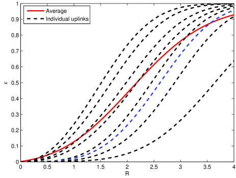
Figure 2: Outage probability of eight randomly selected uplinks (dashed lines) along with the average outage probability for the entire network (solid line). The results are for a half-loaded network ($M/C=G/2$), with distance-dependent fading and shadowing ($\sigma_{s}=8$ dB) and are shown as a function of the rate $R$.

Fig. 2 shows the outage probability as a function of rate. Assuming the use of a capacity-approaching code, two-dimensional signaling over an AWGN channel, and Gaussian interference, the SINR threshold corresponding to rate $R$ is $\beta=2^{R}-1$. The dashed lines in Fig. 2 were generated by selecting eight random uplinks and computing the outage probability for each using this threshold. Despite the use of power control, there is considerable variability in the outage probability. The outage probabilities {$\epsilon_{i}\}$ were computed for all $M$ uplinks in the system, and the average outage probability,

$$\mathbb{E}[\epsilon]=\frac{1}{M}\sum_{i=1}^{M}\epsilon_{i}$$ (17)

is displayed as a solid line in the figure.

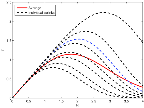
Figure 3: Throughput of eight randomly selected uplinks (dashed lines) along with the average throughput for the entire network (solid line). System parameters are the same used to generate Fig. 2.

Fig. 3 shows the throughput as a function of rate, where the throughput of the $i^{th}$ uplink is found as

$$T_{i}=R_{i}(1-\epsilon_{i})$$ (18)

and represents the rate of successful transmissions. The parameters are the same as those used to produce Fig. 2, and again the SINR threshold corresponding to rate $R$ is $\beta=2^{R}-1$. The plot shows the throughput for the same eight uplinks whose outage was shown in Fig. 2, as well as the average throughput

$$\mathbb{E}[T]=\frac{1}{M}\sum_{i=1}^{M}R_{i}(1-\epsilon_{i}).$$ (19)

IV-B1 Fixed-Rate Policies

Consider the case that all uplinks in the system must use the same rate; i.e., $R_{i}=R$, for all uplinks. On the one hand, the rate could be selected to maximize the average throughput. With respect to the example shown in Fig. 3, this corresponds to selecting the $R$ that maximizes the solid curve, which occurs at $R=1.81$. However, at the rate that maximizes throughput, the corresponding outage probability could be unacceptably high. When $R=1.81$ in the example, the corresponding average outage probability is $\mathbb{E}[\epsilon]=0.37$, which is too high for many applications. As an alternative to maximizing throughput, the rate $R$ could be selected to satisfy an outage constraint $\zeta$ so that $\mathbb{E}[\epsilon]\leq\zeta$. For instance, setting $R=0.84$ in the example satisfies an average outage constraint $\zeta=0.1$ with equality. To distinguish between the two fixed-rate policies, we call the first policy maximal-throughput fixed rate (MTFR) and the second policy outage-constrained fixed rate (OCFR).

IV-B2 Variable-Rate Policies

If $R$ is selected to satisfy an average outage constraint, the outage probability of the individual uplinks will vary around this average. Furthermore, selecting $R$ to maximize the average throughput does not generally maximize the throughput of the individual uplinks. These issues can be alleviated by selecting the rates $R_{i}$ independently for the different uplinks. The rates could be selected to maximize the throughput of each uplink; i.e., $R_{i}=\arg\max T_{i}$ for each uplink, where the maximization is over all possible rates. We call this the maximal-throughput variable-rate (MTVR) policy. Alternatively, the selection could be made to require all uplinks to satisfy the outage constraint $\zeta$; i.e., $\epsilon_{i}\leq\zeta$ for all $i$. We call this the outage-constrained variable-rate (OCVR) policy.

V Performance Analysis

V-A Performance Metrics

While the outage probability, throughput, and rate characterize the performance of a single uplink, they do not quantify the total data flow in the network because they do not account for the number of uplink users that are served. By taking into account the number of mobiles per unit area, the total data flow in a given area can be characterized by the transmission capacity, defined as [12]

$$\tau=\lambda\mathbb{E}[T]=\lambda\mathbb{E}\left[\left(1-\epsilon\right)R\right]$$ (20)

where $\lambda=M/\pi r_{\mathsf{net}}^{2}$ is the density of transmissions in the network, and the units are bits per channel use per unit area. Transmission capacity can be interpreted as the spatial intensity of transmissions; i.e., the rate of successful data transmission per unit area.

Performance metrics can be obtained using a Monte Carlo approach as follows. Draw a realization of the network by placing $C$ base stations and $M$ mobiles within the disk of radius $r_{\mathsf{net}}$ according to the uniform clustering model with minimum base-station separation $r_{\mathsf{bs}}$ and minimum mobile separation $r_{\mathsf{m}}$. Compute the path loss from each base station to each mobile, applying randomly generated shadowing factors. Determine the set of mobiles associated with each cell sector. Assuming that the number of mobiles served in a cell sector cannot exceed $G$, which is the number of orthogonal sequences available for the downlink, then set the rate of the last $M_{j}-G$ mobiles in the cell sector (if there are that many) to zero (since they will be denied access). At each sector antenna, apply the power-control policy to determine the power it receives from each mobile that it serves. For each cell sector, compute the rates, outage probabilities, and throughputs according to the MTFR, OCFR, MTVR, or OCVR network policy. Then compute the transmission capacity.

V-B Simulation Parameters

In the following subsections, the Monte Carlo method described in the previous subsection is used to characterize the uplink performance. In all cases considered, the network has $C=50$ base stations placed in a circular network of radius $r_{\mathsf{net}}=2$. Except for Subsection V-E, which studies the influence of $r_{\mathsf{bs}}$, the base-station exclusion zones are set to have radius $r_{\mathsf{bs}}=0.25$. A variable number $M$ of mobiles are placed within the network using exclusion zones of radius $r_{\mathsf{m}}=0.01$. The SNR is $\Gamma=10$ dB, and the activity factor is $p_{i}=1$. Unless otherwise stated, the path-loss exponent is $\alpha=3$. The fading is the distance-dependent fading specified by (16). Both unshadowed and shadowed ($\sigma_{s}=8$ dB) environments are considered. The chip factor is $h=2/3$, and except for Subsection V-D, which studies the influence of $G$, the spreading factor is $G=16$.

V-C Policy Comparison

Fig. 4 shows the average transmission capacity of the four network policies in distance-dependent fading, both with and without shadowing, as a function of the load $M/C$. For the OCFR policy, the average was obtained by optimizing over a rate that is common to all sectors. For the OCVR policy, the uplink rate $R_{i}$ of each uplink was maximized subject to an outage constraint. While the transmission capacities of the MTFR and MTVR policies are potentially superior to those of the OCFR and OCVR policies, this advantage comes at the cost of a variable and high value of $\epsilon$, which is generally too large for most applications. The bottom pair of curves in Fig. 4 indicate that the OCVR policy has a higher average transmission capacity than the OCFR policy.

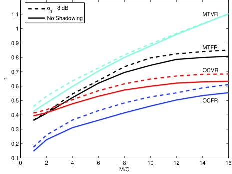
Figure 4: Transmission capacity for the four network policies as function of the load $M/C$ for distance-dependent fading and both shadowed ($\sigma_{s}=$ 8 dB) and unshadowed cases, assuming that the rates are optimized.

V-D Spreading Factor

Fig. 5 shows the transmission capacity as a function of the spreading factor $G$ (with $h=2/3$) for the shadowed distance-dependent-fading channel. Two loads are shown for each of the four policies. An increase in $G$ is beneficial for all policies, but the MTVR policy benefits the most.

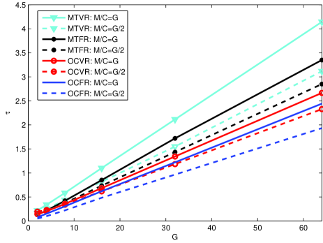
Figure 5: Transmission capacity as function of spreading factor $G$ for two values of system load, distance-dependent fading, and shadowing with $\sigma_{s}=8$ dB.

V-E Base-Station Exclusion Zone

Fig. 6 shows the transmission capacity for each of the four policies as a function of the base-station exclusion zone $r_{\mathsf{bs}}$ for $M/C=G/2$ and two values of path-loss exponent $\alpha$. The distance-dependent fading model is used, and shadowing is applied with $\sigma_{s}=$ 8 dB. The two policies that constrain the outage probability are more sensitive to the value of $r_{\mathsf{bs}}$ than the two policies that maximize throughput.

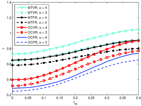
Figure 6: Transmission capacity as a function of the base-station exclusion zone $r_{\mathsf{bs}}$ for four policies and two values of path-loss exponent $\alpha$.

VI Conclusion

A new analysis of DS-CDMA uplinks has been presented. This analysis is much more detailed and accurate than existing ones and facilitates the resolution of network design issues. In particular, it has been shown that once power control is established, the rate can be allocated according to a fixed-rate or variable-rate policy with the objective of either maximizing throughput or meeting an outage constraint. An advantage of variable-rate power control is that it allows an outage constraint to be enforced on every uplink, which is impossible when a fixed rate is used throughout the network. Another advantage is an increased transmission capacity.

References

- [1] K. S. Gilhousen et al., “On the capacity of a cellular CDMA system,” IEEE Trans. Veh. Technol., vol. 40, pp. 303–312, May 1991.
- [2] A. J. Viterbi, CDMA Principles of Spread Spectrum Communication. Addison-Wesley, 1995.
- [3] M. Zorzi, “On the Analytical Computation of the Interference Statistics with Applications to the Performance Evaluation of Mobile Radio Systems,” IEEE Trans. Commun., vol. 45, pp. 103–109, Jan. 1997.
- [4] J. Andrews, F. Baccelli, and R. K. Ganti, “A tractable approach to coverage and rate in cellular networks,” IEEE Trans. Commun., vol. 59, pp. 3122–3134, Nov. 2011.
- [5] H. S. Dhillon, T. D. Novlan, and J. G. Andrews, “Coverage Probability of Uplink Cellular Networks,” in Proc. GLOBECOM, Dec. 2012.
- [6] S. Stoyan, W. Kendall, and J. Mecke, Stochastic Geometry and Its Applications. Wiley, 1996.
- [7] F. Baccelli and B. Blaszczyszyn, Stochastic Geometry and Wireless Networks. NOW: Foundations and Trends in Networking, 2010.
- [8] D. Torrieri and M. C. Valenti, “The outage probability of a finite ad hoc network in Nakagami fading,” IEEE Trans. Commun., Nov. 2012.
- [9] M. C. Valenti, D. Torrieri, and S. Talarico, “A New Analysis of the DS-CDMA Cellular Downlink Under Spatial Constraints,” Proc. ICNC, Jan. 2013.
- [10] D. Torrieri, Principles of Spread-Spectrum Communication Systems, 2nd ed. Springer, 2011.
- [11] D. Torrieri, “Performance of direct-sequence systems with long pseudonoise sequences,” IEEE J. Selected Areas Commun., vol. 10, pp. 770-781, May 1992.
- [12] S. Weber, J. G. Andrews, and N. Jindal, “An overview of the transmission capacity of wireless networks,” IEEE Trans. Commun., vol. 58, pp. 3593–3604, Dec. 2010.