Bethe Vectors of Quantum Integrable Models with GL(3) Trigonometric $R$-Matrix

Bethe Vectors of Quantum Integrable Models
with GL(3) Trigonometric $\boldsymbol{R}$-Matrix

Samuel BELLIARD ${}^{{\dagger}^{1}}\!$, Stanislav PAKULIAK ${}^{{\dagger}^{2}{\dagger}^{3}{\dagger}^{4}}\!$, Eric RAGOUCY ${}^{{\dagger}^{5}}\!$, Nikita A. SLAVNOV ${}^{{\dagger}^{6}}$ S. Belliard, S. Pakuliak, E. Ragoucy and N.A. Slavnov

${}^{{\dagger}^{1}}$ Université Montpellier 2, Laboratoire Charles Coulomb,
${}^{{\dagger}^{1}}$ UMR 5221, F-34095 Montpellier, France samuel.belliard@univ-montp2.fr

${}^{{\dagger}^{2}}$ Laboratory of Theoretical Physics, JINR, 141980 Dubna, Moscow reg., Russia pakuliak@theor.jinr.ru ${}^{{\dagger}^{3}}$ Moscow Institute of Physics and Technology, 141700 Dolgoprudny, Moscow reg., Russia ${}^{{\dagger}^{4}}$ Institute of Theoretical and Experimental Physics, 117259 Moscow, Russia

${}^{{\dagger}^{5}}$ Laboratoire de Physique Théorique LAPTH, CNRS and Université de Savoie,
${}^{{\dagger}^{5}}$ BP 110, 74941 Annecy-le-Vieux Cedex, France eric.ragoucy@lapth.cnrs.fr

${}^{{\dagger}^{6}}$ Steklov Mathematical Institute, Moscow, Russia nslavnov@mi.ras.ru

Received May 27, 2013, in final form September 27, 2013; Published online October 07, 2013

We study quantum integrable models with ${\rm GL}(3)$ trigonometric $R$-matrix and solvable by the nested algebraic Bethe ansatz. Using the presentation of the universal Bethe vectors in terms of projections of products of the currents of the quantum affine algebra $U_{q}(\widehat{\mathfrak{gl}}_{3})$ onto intersections of different types of Borel subalgebras, we prove that the set of the nested Bethe vectors is closed under the action of the elements of the monodromy matrix.

nested algebraic Bethe ansatz; Bethe vector; current algebra

81R50; 17B80

1 Introduction

We consider a quantum integrable model defined by the monodromy matrix $T(u)$ with matrix elements $T_{ij}(u)$, $i,j=1,2,3$, which satisfies the commutation relation

$${\rm R}(u,v)\cdot(T(u)\otimes\mathbf{1})\cdot(\mathbf{1}\otimes T(v))=(\mathbf{1}\otimes T(v))\cdot(T(u)\otimes\mathbf{1})\cdot{\rm R}(u,v),$$ (1.1)

with the $U_{q}(\widehat{\mathfrak{gl}}_{3})$ trigonometric quantum $R$-matrix

$${\rm R}(u,v)={\sf f}(u,v)\sum_{1\leq i\leq 3}{\sf E}_{ii}\otimes{\sf E}_{ii}+\sum_{1\leq i<j\leq 3}({\sf E}_{ii}\otimes{\sf E}_{jj}+{\sf E}_{jj}\otimes{\sf E}_{ii})$$

$$\phantom{{\rm R}(u,v)=}{}+\sum_{1\leq i<j\leq 3}\big{(}u{\sf g}(u,v){\sf E}_{ij}\otimes{\sf E}_{ji}+v{\sf g}(u,v){\sf E}_{ji}\otimes{\sf E}_{ij}\big{)}.$$ (1.2)

Here the rational functions ${\sf f}(u,v)$ and ${\sf g}(u,v)$ are

$${\sf f}(u,v)=\frac{qu-q^{-1}v}{u-v},\qquad{\sf g}(u,v)=\frac{\big{(}q-q^{-1}\big{)}}{u-v},$$

and $({\sf E}_{ij})_{lk}=\delta_{il}\delta_{jk}$, $i,j,l,k=1,2,3$ are $3\times 3$ matrices with unit in the intersection of the $i$th row and the $j$th column and zero matrix elements elsewhere. The $R$-matrix (1.2) is called ‘trigonometric’ because its classical limit gives the classical trigonometric $r$-matrix [1]. The trigonometric $R$-matrix (1.2) is written in multiplicative variables and depends actually on the ratio $u/v$ of these multiplicative parameters.

Due to the commutation relation (1.1) the transfer matrix $t(u)=\operatorname{tr}T(u)=T_{11}(u)+T_{22}(u)+T_{33}(u)$ generates a set of commuting integrals of motion and the first step of the algebraic Bethe ansatz [9] is the construction of the set of eigenstates for these commuting operators in terms of the monodromy matrix entries. We assume that these matrix elements act in a quantum space $V$ and that this space possesses a vector $|0\rangle\in V$ such that

$$T_{ij}(u)|0\rangle=0,\quad i>j,\qquad T_{ii}(u)|0\rangle=\lambda_{i}(u)|0\rangle,\qquad\lambda_{i}(u)\in{\mathbb{C}}\big{[}\big{[}u,u^{-1}\big{]}\big{]}.$$

The eigenstates ${\mathbb{B}}^{a,b}(\bar{u};\bar{v})$ of the transfer matrix $t(u)$ in quantum integrable models with ${\rm GL}(3)$ trigonometric $R$-matrix depend on two sets of variables

$$\bar{u}=\left\{u_{1},\ldots,u_{a}\right\},\qquad\bar{v}=\left\{v_{1},\ldots,v_{b}\right\},$$

which are called the Bethe parameters. These eigenstates can be constructed in the framework of the nested Bethe ansatz method formulated in [19] and are given by certain polynomials in the monodromy matrix elements $T_{12}(u)$, $T_{23}(u)$, $T_{13}(u)$ with rational coefficients depending on the Bethe parameters.

In pioneer papers on nested Bethe ansatz [17, 18, 19] no explicit formulae for the Bethe vectors were obtained. The method, in its original formulation, allows one to get the Bethe equations by requiring that the Bethe vectors are eigenstates of the transfer matrix. Nevertheless, even when the Bethe parameters are free and do not satisfy any restrictions, the structure of the Bethe vectors (sometimes such Bethe vectors are called off-shell) is rather complicated. More explicit formulae for the off-shell nested Bethe vectors were obtained in [26] in the theory of solutions of the quantum Knizhnik–Zamolodchikov equation. The Bethe vectors were given by certain traces over auxiliary spaces of the products of the monodromy matrices and $R$-matrices. This presentation allows one to investigate the structure of the nested off-shell Bethe vectors and to obtain the explicit formulae for the nested Bethe vectors when the space $V$ becomes a tensor product of evaluation representations of the Yangian and of the positive Borel subalgebra of the quantum affine algebra $U_{q}(\widehat{\mathfrak{gl}}_{N})$ [25].

Explicit expressions for the off-shell nested Bethe vectors in the ${\rm GL}(N)$ quantum integrable models in terms of the monodromy matrix elements were obtained in the papers [12, 14, 21], where the realization of these vectors in terms of the current generators of the quantum affine algebra $U_{q}(\widehat{\mathfrak{gl}}_{N})$ [7] was used. This realization uses the notion of projections onto intersections of different types of Borel subalgebras in the quantum affine algebras introduced firstly in [8]. Of course, it also uses the isomorphism between the current [6] and the $L$-operator formulations of the quantum affine algebras [23] investigated in [5].

Quite analogously one can construct dual off-shell Bethe vectors ${\mathbb{C}}^{a,b}(\bar{u};\bar{v})$ defined in the dual space $V^{*}$ with the dual vacuum vector $\langle 0|\in V^{*}$:

$$\langle 0|T_{ij}(u)=0,\quad i<j,\qquad\langle 0|T_{ii}(u)=\lambda_{i}(u)\langle 0|.$$

They can be also explicitly written as polynomials in the monodromy matrix elements $T_{21}(u)$, $T_{32}(u)$, $T_{31}(u)$ with rational coefficients using the current realization of the quantum affine algebra $U_{q}(\widehat{\mathfrak{gl}}_{3})$ [2].

For the class of nested quantum integrable models where the inverse scattering problem can be solved and local operators can be expressed in terms of the monodromy matrix elements [20], one can now address the problem of calculation of the form factors and the correlation functions of local operators. It was done in [16] for the quantum integrable models with ${\rm GL}(2)$ trigonometric $R$-matrix, using determinant formulae for the scalar products of the Bethe vectors obtained in [24].

To approach this problem one has to answer the following question. Whether the action of the monodromy matrix elements onto nested off-shell Bethe vectors produces linear combinations of vectors with the same structure. If this is true, then the problem of computing the form factors of local operators can be reduced to the calculation of the scalar products between off-shell and on-shell Bethe vectors. Moreover, since right and left Bethe vectors are presented as linear combinations of products of the monodromy matrix elements, the calculation of these scalar products itself can be also reduced to the application of the action formulae of the monodromy matrix elements onto Bethe vectors.

The goal of this paper is to give a positive answer to this question and to present and prove the explicit formulae for such an action. We should say that in case of quantum integrable models with ${\rm GL}(2)$ $R$-matrix, the question about the action formulae is almost trivial, since the right and left off-shell Bethe vectors in this case are given by the product of the monodromy matrix elements $T_{12}(u)$ and $T_{21}(u)$ respectively. These action formulae can be easily extracted from the $RTT$ relation (1.1) for the monodromy operators. In higher-rank systems, due to the nontrivial structure of the nested Bethe vectors, the application of the $RTT$ relations for the calculation of the action formulae becomes a very complicated combinatorial problem. In the following, to solve it, we will use the presentation of the nested off-shell Bethe vectors in terms of the current generators of the quantum affine algebra $U_{q}(\widehat{\mathfrak{gl}}_{3})$ and the relation between the monodromy matrix elements and the current generators given by the Gauss decomposition.

2 Quantum affine algebra $\boldsymbol{U_{q}(\widehat{\mathfrak{gl}}_{3})}$

In order to reach the goal of the paper, rather than working with a specific quantum integrable model whose monodromy matrix satisfies the commutation relations (1.1), we deal with a more abstract situation. We consider the universal monodromy matrix which coincides with the $L$-operator of the positive Borel subalgebra of the quantum affine algebra $U_{q}(\widehat{\mathfrak{gl}}_{3})$. There exists an isomorphism [5] between the $L$-operators [23] and the current [6] formulations of this algebra. The expression of the universal Bethe vectors in terms of the current generators was computed in [12], see also equations (3.5), (3.6) below. Using these data, we will calculate the action of the monodromy matrix elements onto these Bethe vectors using essentially the commutations relations of the algebra $U_{q}(\widehat{\mathfrak{gl}}_{3})$ in the current realization. The aim of this section is to introduce these algebraic objects.

2.1 Two realizations of $\boldsymbol{U_{q}(\widehat{\mathfrak{gl}}_{3})}$

The quantum affine algebra $U_{q}(\widehat{\mathfrak{gl}}_{3})$ is an associative algebra with unit. In the $L$-operator formulation [23] it is generated by the modes ${L}^{\pm}_{ij}[n]$, $i,j=1,2,3$, $n\geq 0$ such that

$${L}^{+}_{ji}[0]={L}^{-}_{ij}[0]=0,\qquad 1\leq i<j\leq 3.$$ (2.1)

These modes can be gathered into the generating series

$${L}^{\pm}(u)=\sum_{n\geq 0}\sum_{i,j=1}^{3}{\sf E}_{ij}\otimes{L}^{\pm}_{ij}[n]u^{\mp n}\in\text{End}\big{(}{\mathbb{C}}^{3}\big{)}\otimes U_{q}(\mathfrak{b}_{\pm}),$$ (2.2)

where $U_{q}(\mathfrak{b}_{\pm})\subset U_{q}(\widehat{\mathfrak{gl}}_{3})$ are the positive and negative Borel subalgebras of the quantum affine algebra $U_{q}(\widehat{\mathfrak{gl}}_{3})$. These generating series can be called universal monodromy matrices since they satisfy the same as (1.1) commutation relation

$${\rm R}(u,v)\cdot\big{(}{L}^{\mu}(u)\otimes\mathbf{1}\big{)}\cdot(\mathbf{1}\otimes{L}^{\nu}(v))=(\mathbf{1}\otimes{L}^{\nu}(v))\cdot({L}^{\mu}(u)\otimes\mathbf{1})\cdot{\rm R}(u,v),$$ (2.3)

where $\mu,\nu=\pm$.

The quantum affine algebra $U_{q}(\widehat{\mathfrak{gl}}_{3})$ is a Hopf algebra and the Borel subalgebras generated by the modes of the $L$-operators ${L}^{\pm}(u)$ are Hopf subalgebras for the standard coproduct

$$\Delta\left({L}_{ij}^{\pm}(u)\right)=\sum_{k=1}^{3}{L}^{\pm}_{kj}(u)\otimes{L}^{\pm}_{ik}(u).$$

In what follows we will need another realization of the same algebra, the so-called current realization of the quantum affine algebra $U_{q}(\widehat{\mathfrak{gl}}_{3})$ given in [6]. To relate the current and $L$-operator realizations of the same algebra we introduce, according to [5], the Gauss decomposition of the $L$-operator

$${L}^{\pm}(u)=\left(\begin{matrix}1&{\rm F}^{\pm}_{21}(u)&{\rm F}^{\pm}_{31}(u)\vspace{1mm}\\ 0&1&{\rm F}^{\pm}_{32}(u)\\ 0&0&1\end{matrix}\right)\left(\begin{matrix}{k}^{\pm}_{1}(u)&0&0\\ 0&{k}^{\pm}_{2}(u)&0\\ 0&0&{k}^{\pm}_{3}(u)\end{matrix}\right)\left(\begin{matrix}1&0&0\\ {\rm E}^{\pm}_{12}(u)&1&0\vspace{1mm}\\ {\rm E}^{\pm}_{13}(u)&{\rm E}^{\pm}_{23}(u)&1\end{matrix}\right),$$ (2.4)

that is to say

$$L^{\pm}_{ab}(u)={\rm F}^{\pm}_{ba}(u){k}^{+}_{b}(u)+\sum_{b<m\leq 3}{\rm F}^{\pm}_{ma}(u){k}^{+}_{m}(t){\rm E}^{\pm}_{bm}(u),\qquad a<b,$$ (2.5)

$$L^{\pm}_{bb}(u)={k}^{\pm}_{b}(u)+\sum_{b<m\leq 3}{\rm F}^{\pm}_{mb}(u){k}^{\pm}_{m}(u){\rm E}^{\pm}_{bm}(u),$$ (2.6)

$$L^{\pm}_{ab}(u)={k}^{\pm}_{a}(u){\rm E}^{\pm}_{ba}(u)+\sum_{a<m\leq 3}{\rm F}^{\pm}_{ma}(u){k}^{\pm}_{m}(u){\rm E}^{\pm}_{bm}(u),\qquad a>b.$$ (2.7)

It was proved in the paper [5] that, after substitution of the decompositions (2.5)–(2.7) into the commutation relations (2.3), one can obtain for the linear combinations of the Gauss coordinates

$${F}_{i}(t)={\rm F}^{+}_{i+1\,i}(t)-{\rm F}^{-}_{i+1\,i}(t),\qquad{E}_{i}(t)={\rm E}^{+}_{i\,i+1}(t)-{\rm E}^{-}_{i\,i+1}(t)$$ (2.8)

and ${k}^{\pm}_{i}(t)$ the following commutation relations:

$$\big{(}q^{-1}z-qw\big{)}{E}_{i}(z){E}_{i}(w)={E}_{i}(w){E}_{i}(z)\big{(}qz-q^{-1}w\big{)},$$ (2.9)

$$(z-w){E}_{i}(z){E}_{i+1}(w)={E}_{i+1}(w){E}_{i}(z)\big{(}q^{-1}z-qw\big{)},$$ (2.10)

$${k}_{i}^{\pm}(z){E}_{i}(w)\left({k}_{i}^{\pm}(z)\right)^{-1}=\frac{z-w}{q^{-1}z-qw}{E}_{i}(w),$$ (2.11)

$${k}_{i+1}^{\pm}(z){E}_{i}(w)\left({k}_{i+1}^{\pm}(z)\right)^{-1}=\frac{z-w}{qz-q^{-1}w}{E}_{i}(w),$$ (2.12)

$${k}_{i}^{\pm}(z){E}_{j}(w)\left({k}_{i}^{\pm}(z)\right)^{-1}={E}_{j}(w),\qquad{\rm if}\quad i\not=j,j+1,$$ (2.13)

$$\big{(}qz-q^{-1}w\big{)}{F}_{i}(z){F}_{i}(w)={F}_{i}(w){F}_{i}(z)\big{(}q^{-1}z-qw\big{)},$$ (2.14)

$$\big{(}q^{-1}z-qw\big{)}{F}_{i}(z){F}_{i+1}(w)={F}_{i+1}(w){F}_{i}(z)(z-w),$$ (2.15)

$${k}_{i}^{\pm}(z){F}_{i}(w)\left({k}_{i}^{\pm}(z)\right)^{-1}=\frac{q^{-1}z-qw}{z-w}{F}_{i}(w),$$ (2.16)

$${k}_{i+1}^{\pm}(z){F}_{i}(w)\left({k}_{i+1}^{\pm}(z)\right)^{-1}=\frac{qz-q^{-1}w}{z-w}{F}_{i}(w),$$ (2.17)

$${k}_{i}^{\pm}(z){F}_{j}(w)\left({k}_{i}^{\pm}(z)\right)^{-1}={F}_{j}(w),\qquad{\rm if}\quad i\not=j,j+1,$$ (2.18)

$$[{E}_{i}(z),{F}_{j}(w)]=\delta_{{i},{j}}\delta(z/w)\big{(}q-q^{-1}\big{)}\left({k}^{+}_{i}(z)/{k}^{+}_{i+1}(z)-{k}^{-}_{i}(w)/{k}^{-}_{i+1}(w)\right),$$ (2.19)

plus the Serre relations for the currents ${E}_{i}(z)$ and ${F}_{i}(z)$ which are unimportant for this paper.

The commutation relations for the algebra $U_{q}(\widehat{\mathfrak{gl}}_{3})$, given in terms of the currents, should be considered as formal series identities describing the infinite set of relations between the modes of these currents. The symbol $\delta(z)$ entering these relations is the formal series $\sum\limits_{n\in{\mathbb{Z}}}z^{n}$.

For any series $G(t)=\sum\limits_{m\in{\mathbb{Z}}}G[m]t^{-m}$ we denote $G(t)^{(+)}=\sum\limits_{m>0}G[m]t^{-m}$, and $G(t)^{(-)}=-\sum\limits_{m\leq 0}G[m]t^{-m}$. Using this notation the Ding–Frenkel formulae (2.8) can be inverted

$${\rm F}^{\pm}_{i+1\,i}(z)=z\left(z^{-1}{F}_{i}(z)\right)^{(\pm)},\qquad{\rm E}^{\pm}_{i\,i+1}(z)={E}_{i}(z)^{(\pm)}.$$ (2.20)

2.2 Different type Borel subalgebras and ordering of current generators

The isomorphism between the $L$-operator [23] and the current [6] formulations of the quantum affine algebra, proved in [5], allows one to express the modes of the $L$-operators through the modes of the currents and vice versa using the initial relation (2.1) and the formulae (2.5)–(2.7). On the other hand, it was proved in [15] that the current generators for the quantum affine algebras form the part of the Cartan–Weyl basis in these algebras.

There exists a natural ordering in the Cartan–Weyl basis. If the generator $e_{\gamma}$ corresponds to a positive root $\gamma=\alpha+\beta$, where $\alpha$ and $\beta$ are roots, then these generators are ordered either in a way $e_{\alpha}\prec e_{\gamma}\prec e_{\beta}$ or in the way $e_{\beta}\prec e_{\gamma}\prec e_{\alpha}$. An important property of the Cartan–Weyl basis of a Borel subalgebra of the quantum algebras is that the $q$-commutator of any two generators from this subalgebra, say $e_{\alpha}$ and $e_{\beta}$, is a linear combination of monomials containing only the products of generator $e_{\gamma_{i}}$ which are ‘between’ $e_{\alpha}$ and $e_{\beta}$:

$$e_{\alpha}\prec e_{\gamma_{i}}\prec e_{\beta}\qquad\text{or}\qquad e_{\alpha}\succ e_{\gamma_{i}}\succ e_{\beta}.$$

This property of the Cartan–Weyl basis allows one to describe easily the subalgebras in the quantum affine algebras. For instance, in the example above all generators corresponding to the roots $\alpha$, $\gamma_{i}$, $\beta$ form a subalgebra by definition. The standard positive Borel subalgebra in $U_{q}(\widehat{\mathfrak{gl}}_{3})$ generated by the modes of $L$-operators (2.2) is formed by the Cartan–Weyl generators which are ‘between’ the affine root generator $e_{\alpha_{0}}$ and non-affine negative simple roots generators $e_{-\alpha_{1}}$ and $e_{-\alpha_{2}}$. Respectively, the negative Borel subalgebra is formed by the generators which are ‘between’ $e_{\alpha_{1}}$, $e_{\alpha_{2}}$ and $e_{-\alpha_{0}}$.

The ordering on the Borel subalgebra can be extended to the ordering of the whole set of Cartan–Weyl generators corresponding to the positive and negative roots such that the same ordering property is valid. This ordering is called ‘circular’ or ‘convex’ and it allows one to order arbitrary monomials in the whole algebra [7].

We consider two types of Borel subalgebras of the algebra $U_{q}(\widehat{\mathfrak{gl}}_{3})$. Standard positive and negative Borel subalgebras $U_{q}(\mathfrak{b}^{\pm})\subset U_{q}(\widehat{\mathfrak{gl}}_{3})$ are generated by the modes of the $L$-operators $L^{(\pm)}(u)$ respectively. For the generators in these subalgebras we can use the modes of the Gauss coordinates (2.5)–(2.7) ${\rm E}^{\pm}_{i\,i+1}(u)$, ${\rm F}^{\pm}_{i+1\,i}(u)$, ${k}^{\pm}_{j}(u)$, $i=1,2$, $j=1,2,3$.

Another type of Borel subalgebras is related to the current realizations of $U_{q}(\widehat{\mathfrak{gl}}_{3})$ given in the previous subsection. The Borel subalgebra $U_{F}\subset U_{q}(\widehat{\mathfrak{gl}}_{3})$ is generated by modes of the currents $F_{i}[n]$, $k^{+}_{j}[m]$, $i=1,2$, $j=1,2,3$, $n\in{\mathbb{Z}}$ and $m\geq 0$. The Borel subalgebra $U_{E}\subset U_{q}(\widehat{\mathfrak{gl}}_{3})$ is generated by the modes of the currents $E_{i}[n]$, $k^{-}_{j}[-m]$, $i=1,2$, $j=1,2,3$, $n\in{\mathbb{Z}}$ and $m\geq 0$. We will consider also a subalgebras $U^{\prime}_{F}=U_{F}\setminus\{k^{+}_{j}[0]\}$ and $U^{\prime}_{E}=U_{E}\setminus\{k^{-}_{j}[0]\}$.

Further, we will be interested in the intersections,

$${U}_{F}^{-}={U}^{\prime}_{F}\cap U_{q}(\mathfrak{b}^{-}),\qquad{U}_{F}^{+}={U}_{F}\cap U_{q}(\mathfrak{b}^{+}),$$

$${U}_{E}^{-}={U}_{E}\cap U_{q}(\mathfrak{b}^{-}),\qquad{U}_{E}^{+}={U}^{\prime}_{E}\cap U_{q}(\mathfrak{b}^{+}),$$

and will describe properties of projections to these intersections. We call $U_{F}$ and $U_{E}$ the current Borel subalgebras. Let $U_{f}\subset U_{F}$ and $U_{e}\subset U_{E}$ be the subalgebras of the current Borel subalgebras generated by the modes of the currents $F_{i}[n]$ and $E_{i}[n]$, $i=1,2$, $n\in{\mathbb{Z}}$ only. In what follows we will use the subalgebras $U^{+}_{f}\subset U_{f}$ and $U^{+}_{e}\subset U_{e}$ defined by the intersections

$$U_{f}^{+}=U^{+}_{F}\cap U_{f}\qquad U_{e}^{+}=U^{+}_{E}\cap U_{e}.$$

Let $U^{\pm}_{k}$ be subalgebras in $U_{q}(\widehat{\mathfrak{gl}}_{3})$ generated by the modes of the Cartan currents $k^{\pm}_{j}(u)$.

We fix a ‘circular’ ordering ‘$\prec$’ on the generators of $\overline{U}_{q}(\mathfrak{gl}_{3})$ (see [7]), such that:

$$\cdots\prec U^{-}_{k}\prec U^{-}_{f}\prec U^{+}_{f}\prec U^{+}_{k}\prec U^{+}_{e}\prec U^{-}_{e}\prec U^{-}_{k}\prec\cdots.$$ (2.21)

The ordering of the subalgebras described above can be pictured in the Fig. 1 in the anti-clockwise direction.

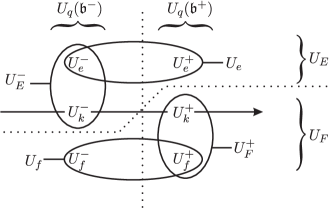
Figure 1: Subalgebras of $\overline{U}_{q}(\mathfrak{gl}_{3})$. The vertical dotted line separates the standard Borel subalgebras. The horizontal dotted line separates the current Borel subalgebras. The horizontal solid axis indicates the increasing of the current generators modes. Ovals denote different subalgebras in the $\overline{U}_{q}(\mathfrak{gl}_{3})$ standard and current Borel subalgebras.

We will call an element $W\in\overline{U}_{q}(\mathfrak{gl}_{3})$ normal ordered and denote it as ${:}W{:}$ if it is presented as linear combinations of products $W_{1}\cdot W_{2}\cdot W_{3}\cdot W_{4}\cdot W_{5}\cdot W_{6}$ such that

$$W_{1}\in U^{-}_{f},\qquad W_{2}\in U^{+}_{f},\qquad W_{3}\in U^{+}_{k},\qquad W_{4}\in U^{+}_{e},\qquad W_{5}\in U^{-}_{e},\qquad W_{6}\in U^{-}_{k}.$$

We may consider the standard Borel subalgebras as ordered with respect to the circular ordering (2.21):

$$U_{q}\big{(}\mathfrak{b}^{-}\big{)}=U^{-}_{e}\cdot U^{-}_{k}\cdot U^{-}_{f},\qquad U_{q}\big{(}\mathfrak{b}^{+}\big{)}=U^{+}_{f}\cdot U^{+}_{k}\cdot U^{+}_{e}.$$

An analogous statement is valid for the current Borel subalgebras:

$$U_{F}=U^{-}_{f}\cdot U^{+}_{f}\cdot U^{+}_{k},\qquad U_{E}=U^{+}_{e}\cdot U^{-}_{e}\cdot U^{-}_{k}.$$

Let us note that the matrix elements in the universal monodromy matrix ${L}^{+}(u)$ given by the formulae (2.5)–(2.7) are normal ordered, i.e. ${:}{L}^{+}(u){:}={L}^{+}(u)$. The problem which we address in this paper, namely the calculation of the action of the monodromy matrix elements onto off-shell Bethe vectors, can be reformulated in the following way. We should put the product of these elements and the element ${P}^{+}_{f}\left({F}_{2}(v_{b})\cdots{F}_{2}(v_{1})\cdot{F}_{1}(u_{a})\cdots{F}_{1}(u_{1})\right)\in U^{+}_{f}$ into its normal order form, modulo terms which annihilate the right vacuum vector $|0\rangle$. Using the Gauss decompositions (2.5)–(2.7), it could be reduced to the commutation of the Gauss coordinates $E^{+}_{ij}(u)$ with the element ${P}^{+}_{f}\left({F}_{2}(v_{b})\cdots{F}_{2}(v_{1})\cdot{F}_{1}(u_{a})\cdots{F}_{1}(u_{1})\right)$. However, this way of doing the normal ordering is almost equivalent to the use of the $RTT$ commutation relations and is far too complicated to be useful for our purpose.

In fact, in this paper, we will employe a different and more efficient strategy: we will use the method of projections introduced in [8] and exploited in a series of papers (see [12] and references therein) to relate the off-shell Bethe vectors with the current realization of the quantum affine algebras. We refer the reader to the above mentioned papers to find a complete theory of the projections onto intersections of the different types of Borel subalgebras. Here, we will give only some short definitions on projections. In order to do this, we need to equip the algebra $U_{q}(\widehat{\mathfrak{gl}}_{3})$ together with its decomposition into current Borel subalgebras by the current Hopf structure

$$\Delta^{(D)}\left({E}_{i}(z)\right)={E}_{i}(z)\otimes 1+{k}^{-}_{i}(z)\left({k}^{-}_{i+1}(z)\right)^{-1}\otimes{E}_{i}(z),$$

$$\Delta^{(D)}\left({F}_{i}(z)\right)=1\otimes{F}_{i}(z)+{F}_{i}(z)\otimes{k}^{+}_{i}(z)\left({k}^{+}_{i+1}(z)\right)^{-1},$$

$$\Delta^{(D)}\left({k}^{\pm}_{i}(z)\right)={k}^{\pm}_{i}(z)\otimes{k}^{\pm}_{i}(z).$$ (2.22)

According to the general theory [7] we introduce the projection operators

$${P}^{\pm}_{f}:U_{F}\subset U_{q}(\widehat{\mathfrak{gl}}_{3})\to U_{F}^{\pm},\qquad{P}^{\pm}_{e}:U_{E}\subset U_{q}(\widehat{\mathfrak{gl}}_{3})\to U_{E}^{\pm}.$$

They are respectively defined by the prescriptions

$${P}^{+}_{f}(f_{-}f_{+})=\varepsilon(f_{-})f_{+},\qquad{P}^{-}_{f}(f_{-}f_{+})=f_{-}\varepsilon(f_{+}),\qquad\forall\,f_{-}\in{U}_{F}^{-},\quad\forall\,f_{+}\in{U}_{F}^{+},$$ (2.23)

$${P}^{+}_{e}(e_{+}e_{-})=e_{+}\varepsilon(e_{-}),\qquad{P}^{-}_{e}(e_{-}e_{+})=\varepsilon(e_{+})e_{-},\qquad\forall\,e_{-}\in{U}_{E}^{-},\quad\forall\,e_{+}\in{U}_{E}^{+},$$ (2.24)

where the counit map $\varepsilon:U_{q}(\widehat{\mathfrak{gl}}_{3})\to{\mathbb{C}}$ is defined on current generators as follows

$$\varepsilon(1)=\varepsilon\big{(}k_{j}^{\pm}(u)\big{)}=1,\qquad\varepsilon(E_{i}(u))=\varepsilon\left(F_{i}(u)\right)=0.$$

Denote by ${\overline{U}}_{F}$ and ${\overline{U}}_{E}$ the extensions of the algebras $U_{F}$ and $U_{E}$ formed by infinite sums of monomials which are ordered products $a_{i_{1}}[n_{1}]\cdots a_{i_{k}}[n_{k}]$ with $n_{1}\leq\cdots\leq n_{k}$, where $a_{i_{l}}[n_{l}]$ is either $F_{i_{l}}[n_{l}]$ or $k^{+}_{i_{l}}[n_{l}]$ and $E_{i_{l}}[n_{l}]$ or $k^{-}_{i_{l}}[n_{l}]$, respectively. It can be checked that

• the action of the projections (2.23) can be extended to the algebra ${\overline{U}}_{F}$;

• for any $f\in{\overline{U}}_{F}$ with $\Delta^{(D)}(f)=\sum\limits_{i}f^{\prime}_{i}\otimes f^{\prime\prime}_{i}$ we have

  $$f=\sum_{i}{P}^{-}_{f}(f^{\prime\prime}_{i})\cdot{P}^{+}_{f}(f^{\prime}_{i});$$ (2.25)

• the action of the projections (2.24) can be extended to the algebra ${\overline{U}}_{E}$;

• for any $e\in{\overline{U}}_{E}$ with $\Delta^{(D)}(e)=\sum\limits_{i}e^{\prime}_{i}\otimes e^{\prime\prime}_{i}$ we have

  $$e=\sum_{i}{P}^{+}_{e}(e^{\prime}_{i})\cdot{P}^{-}_{e}(e^{\prime\prime}_{i}).$$ (2.26)

The formulae (2.25) and (2.26) are the main technical tools to calculate the projections of currents. These formulae allow us to present a product of currents in a normal ordered form using projections and the rather simple current Hopf structure (2.22).

The Ding–Frenkel isomorphism between $L$-operator and current realizations of the quantum affine algebra $U_{q}(\widehat{\mathfrak{gl}}_{N})$ [5] identifies the Gauss coordinates and the full currents through formulae (2.8) and (2.20). It is clear that the Gauss coordinates ${\rm F}^{\pm}_{i+1\,i}(u)={P}^{\pm}_{f}\left(F_{i}(u)\right)$ and ${\rm E}^{\pm}_{i\,i+1}={P}^{\pm}_{e}\left(E_{i}(u)\right)$ are defined by the corresponding projections of the full currents. But there are also higher Gauss coordinates ${\rm F}^{\pm}_{ji}(u)$ and ${\rm E}^{\pm}_{ij}(u)$ for $j>i+1$ and their relation to the currents was not established in [5]. In [12], special elements from the completed algebras $\overline{U}_{F}$ and $\overline{U}_{E}$ were introduced such that their projections yield the corresponding higher Gauss coordinates. These elements were called ‘composed’ currents. In the case of the quantum affine algebra $U_{q}(\widehat{\mathfrak{gl}}_{3})$, there are only two composed currents

$$F_{3,1}(u)\equiv\big{(}q-q^{-1}\big{)}F_{1}(u)F_{2}(u),\qquad E_{1,3}(u)\equiv\big{(}q-q^{-1}\big{)}E_{2}(u)E_{1}(u),$$ (2.27)

such that

$${P}^{+}_{f}\left(F_{3,1}(u)\right)=\big{(}q-q^{-1}\big{)}{\rm F}^{+}_{31}(u),\qquad{P}^{+}_{e}\left(E_{1,3}(u)\right)=\big{(}q-q^{-1}\big{)}{\rm E}^{+}_{13}(u).$$

3 Main results

3.1 Notations

To save space and simplify presentation, we use the following convention for the products of the commuting entries of the monodromy matrix $T_{ij}(w)$, vacuum eigenvalues $\lambda_{i}(w)$ and their ratios ${\sf r}_{k}(w)=\lambda_{k}(w)/\lambda_{2}(w)$, $k=1,3$. Namely, whenever such an operator or a scalar function depends on a set of variables (for instance, $T_{ij}(\bar{w})$, $\lambda_{i}(\bar{u})$, ${\sf r}_{k}(\bar{v})$), this means that we deal with the product of the operators or scalar functions with respect to the corresponding set:

$$T_{ij}(\bar{w})=\prod_{w_{k}\in\bar{w}}T_{ij}(w_{k});\qquad\lambda_{2}(\bar{u})=\prod_{u_{j}\in\bar{u}}\lambda_{2}(u_{j});\qquad{\sf r}_{k}(\bar{v}_{\ell})=\prod_{\begin{subarray}{c}v_{j}\in\bar{v}\\ v_{j}\neq v_{\ell}\end{subarray}}{\sf r}_{k}(v_{j}).$$

A similar convention will be used for the products of functions ${\sf f}(u,v)$ and ${\sf g}(u,v)$

$${\sf f}(w_{i},\bar{w}_{i})=\prod_{\begin{subarray}{c}w_{j}\in\bar{w}\\ w_{j}\neq w_{i}\end{subarray}}{\sf f}(w_{i},w_{j});\qquad{\sf g}(\bar{u},\bar{v})=\prod_{u_{j}\in\bar{u}}\prod_{v_{k}\in\bar{v}}{\sf g}(u_{j},v_{k}).$$

The notation $\bar{v}_{\ell}$ for an arbitrary set $\bar{v}$ means the set $\bar{v}\setminus\{v_{\ell}$}. We will also use the sets $\bar{w}_{<j}=\{w_{1},...,w_{j-1}\}$ and $\bar{w}_{>j}=\bar{w}_{j}\setminus\bar{w}_{<j}$ with obvious convention for the products. Partitions of sets will be noted as $\bar{u}\Rightarrow\{\bar{u}_{\scriptscriptstyle\rm I},\,\bar{u}_{\scriptscriptstyle\rm II}\}$.

To simplify further formulae we will introduce a special notation for product of non-commuting currents:

$${\cal F}_{1}(\bar{u})={F}_{1}(u_{a}){F}_{1}(u_{a-1})\cdots{F}_{1}(u_{1}),\qquad{\cal F}_{2}(\bar{v})={F}_{2}(v_{b})\cdots{F}_{2}(v_{2}){F}_{2}(v_{1})$$ (3.1)

and

$${\cal F}_{1}(\bar{u}_{j})={F}_{1}(u_{a})\cdots{F}_{1}(u_{j+1}){F}_{1}(u_{j-1})\cdots{F}_{1}(u_{1}),$$

$${\cal F}_{2}(\bar{v}_{i})={F}_{2}(v_{b})\cdots{F}_{2}(v_{i+1}){F}_{2}(v_{i-1})\cdots{F}_{2}(v_{1}).$$ (3.2)

These notations are in accordance with the one used for commuting objects, except that now one needs to specify the order as prescribed in (3.1) and (3.2).

In various formulae below the Izergin determinant ${\sf K}_{k}(\bar{x}|\bar{y})$ appears [11]. It is defined for two sets $\bar{x}$ and $\bar{y}$ of the same cardinality $\#\bar{x}=\#\bar{y}=k$:

$${\sf K}_{k}(\bar{x}|\bar{y})=\frac{\prod\limits_{1\leq i,j\leq k}(qx_{i}-q^{-1}y_{j})}{\prod\limits_{1\leq i<j\leq k}(x_{i}-x_{j})(y_{j}-y_{i})}\cdot\det\left[\frac{q-q^{-1}}{(x_{i}-y_{j})(qx_{i}-q^{-1}y_{j})}\right].$$ (3.3)

Below we also use two modifications of the Izergin determinant

$${\sf K}^{(l)}_{k}(\bar{x}|\bar{y})=\prod_{i=1}^{k}x_{i}\cdot{\sf K}_{k}(\bar{x}|\bar{y}),\qquad{\sf K}^{(r)}_{k}(\bar{x}|\bar{y})=\prod_{i=1}^{k}y_{i}\cdot{\sf K}_{k}(\bar{x}|\bar{y}).$$ (3.4)

Some properties of the Izergin determinant and its modifications are gathered into Appendix A.

3.2 Explicit expression for Bethe vectors

The right and left off-shell Bethe vectors can be presented using the current realization of the quantum affine algebra $U_{q}(\widehat{\mathfrak{gl}}_{3})$ [12]

$${\mathbb{B}}^{a,b}(\bar{u};\bar{v})=\frac{\beta(\bar{u}|\bar{v})}{{\sf f}(\bar{v},\bar{u})}{P}^{+}_{f}\left({F}_{2}(v_{b})\cdots{F}_{2}(v_{1})\cdot{F}_{1}(u_{a})\cdots{F}_{1}(u_{1})\right)\cdot{\sf r}_{3}(\bar{v})|0\rangle,$$ (3.5)

$${\mathbb{C}}^{a,b}(\bar{u};\bar{v})=\frac{\beta(\bar{u}|\bar{v})}{{\sf f}(\bar{v},\bar{u})}\langle 0|{\sf r}_{3}(\bar{v}){P}^{+}_{e}\left({E}_{1}(u_{1})\cdots{E}_{1}(u_{a})\cdot{E}_{2}(v_{1})\cdots{E}_{2}(v_{b})\right),$$ (3.6)

where

$$\beta(\bar{u}|\bar{v})=\prod_{1\leq\ell<\ell^{\prime}\leq a}{\sf f}(u_{\ell^{\prime}},u_{\ell})\prod_{1\leq\ell<\ell^{\prime}\leq b}{\sf f}(v_{\ell^{\prime}},v_{\ell}),$$

and ${P}^{+}_{f}$ and ${P}^{+}_{e}$ are projections onto subalgebras of $U_{q}(\widehat{\mathfrak{gl}}_{3})$ generated by the non-negative and positive modes of the simple root currents ${F}_{i}(u)$ and ${E}_{i}(u)$, $i=1,2$, respectively. These projections onto subalgebras in the positive Borel subalgebra of $U_{q}(\widehat{\mathfrak{gl}}_{3})$ were introduced in [8] and their detailed theory was developed in [7]. The formal definition of these projections is given in the present paper through the formulae (2.23) and (2.24).

In what follows we will consider the action of the universal monodromy matrix elements expressed in terms of the Gauss coordinates (2.4) or in terms of the current generators of the quantum affine algebra $U_{q}(\widehat{\mathfrak{gl}}_{3})$ onto universal off-shell Bethe vectors (3.5). To obtain explicit formulae for this action we do not need to calculate the projection in (3.5), but use a special presentation for this projection found in [10] (see also (4.2) below). Using this presentation we only need the commutation relations of the total currents which are much more simple than the $RTT$-relations or the relations between Gauss coordinates.

Note that the function $\beta(\bar{u}|\bar{v})$ removes all the poles and zeros which originate from the product of currents of the same type, while the product of functions ${\sf f}(\bar{v},\bar{u})$ removes all the poles which originate from the product of currents of different types. Indeed, the product ${F}_{i}(u_{2}){F}_{i}(u_{1})$ has a simple pole at the point $u_{1}=q^{2}u_{2}$ and a simple zero at $u_{1}=u_{2}$, while the product ${F}_{2}(v){F}_{1}(u)$ has a simple pole at the point $u=v$. These ‘analytical’ properties of the product of currents are determined by the commutation relations (2.14), (2.15) and were explained in details in the papers [12, 21] using the notion of ordering of the current generators.

3.3 Multiple action of $\boldsymbol{T_{ij}(\bar{w})}$ operators on Bethe vectors

Now we give the main result of this paper, namely a complete list of the multiple actions of the operators $T_{ij}(\bar{w})$ onto the Bethe vectors $\mathbb{B}^{a,b}(\bar{u};\bar{v})$.

Proposition 3.1.

Throughout the proposition, we denote $\{\bar{v},\bar{w}\}=\bar{\xi}$, $\{\bar{u},\bar{w}\}=\bar{\eta}$ and $\#\bar{w}=n$.

The multiple actions of the $T_{ij}(\bar{w})$ operators onto the Bethe vectors $\mathbb{B}^{a,b}(\bar{u};\bar{v})$ are given by:

• Multiple action of $T_{13}$

  $$T_{13}(\bar{w})\mathbb{B}^{a,b}(\bar{u};\bar{v})=\lambda_{2}(\bar{w})\,\mathbb{B}^{a+n,b+n}(\bar{\eta};\bar{\xi}).$$ (3.7)

• Multiple action of $T_{12}$

  $$T_{12}(\bar{w})\mathbb{B}^{a,b}(\bar{u};\bar{v})=\lambda_{2}(\bar{w})\sum\frac{{\sf f}(\bar{\xi}_{\scriptscriptstyle\rm II},\bar{\xi}_{\scriptscriptstyle\rm I})}{{\sf f}(\bar{w},\bar{\xi}_{\scriptscriptstyle\rm I})}{\sf K}^{(r)}_{n}(\bar{w}|\bar{\xi}_{\scriptscriptstyle\rm I})\,\mathbb{B}^{a+n,b}(\bar{\eta};\bar{\xi}_{\scriptscriptstyle\rm II}).$$ (3.8)

  The sum is taken over partitions of $\bar{\xi}\Rightarrow\{\bar{\xi}_{\scriptscriptstyle\rm I},\bar{\xi}_{\scriptscriptstyle\rm II}\}$ with $\#\bar{\xi}_{\scriptscriptstyle\rm I}=n$.

• Multiple action of $T_{23}$

  $$T_{23}(\bar{w})\mathbb{B}^{a,b}(\bar{u};\bar{v})=\lambda_{2}(\bar{w})\sum\frac{{\sf f}(\bar{\eta}_{\scriptscriptstyle\rm I},\bar{\eta}_{\scriptscriptstyle\rm II})}{{\sf f}(\bar{\eta}_{\scriptscriptstyle\rm I},\bar{w})}{\sf K}^{(l)}_{n}(\bar{\eta}_{\scriptscriptstyle\rm I}|\bar{w})\,\mathbb{B}^{a,b+n}(\bar{\eta}_{\scriptscriptstyle\rm II};\bar{\xi}).$$ (3.9)

  The sum is taken over partitions of $\bar{\eta}\Rightarrow\{\bar{\eta}_{\scriptscriptstyle\rm I},\bar{\eta}_{\scriptscriptstyle\rm II}\}$ with $\#\bar{\eta}_{\scriptscriptstyle\rm I}=n$.

• Multiple action of $T_{22}$

  $$T_{22}(\bar{w})\mathbb{B}^{a,b}(\bar{u};\bar{v})=\lambda_{2}(\bar{w})\sum\frac{{\sf f}(\bar{\xi}_{\scriptscriptstyle\rm II},\bar{\xi}_{\scriptscriptstyle\rm I}){\sf f}(\bar{\eta}_{\scriptscriptstyle\rm I},\bar{\eta}_{\scriptscriptstyle\rm II})}{{\sf f}(\bar{w},\bar{\xi}_{\scriptscriptstyle\rm I}){\sf f}(\bar{\eta}_{\scriptscriptstyle\rm I},\bar{w})}{\sf K}^{(r)}_{n}(\bar{w}|\bar{\xi}_{\scriptscriptstyle\rm I})\,{\sf K}^{(l)}_{n}(\bar{\eta}_{\scriptscriptstyle\rm I}|\bar{w})\,\mathbb{B}^{a,b}(\bar{\eta}_{\scriptscriptstyle\rm II};\bar{\xi}_{\scriptscriptstyle\rm II}).$$ (3.10)

  The sum is taken over partitions of: $\bar{\eta}\Rightarrow\{\bar{\eta}_{\scriptscriptstyle\rm I},\bar{\eta}_{\scriptscriptstyle\rm II}\}$ with $\#\bar{\eta}_{\scriptscriptstyle\rm I}=n$; $\bar{\xi}\Rightarrow\{\bar{\xi}_{\scriptscriptstyle\rm I},\bar{\xi}_{\scriptscriptstyle\rm II}\}$ with $\#\bar{\xi}_{\scriptscriptstyle\rm I}=n$.

• Multiple action of $T_{11}$

  $$T_{11}(\bar{w})\mathbb{B}^{a,b}(\bar{u};\bar{v})$$

  $$\qquad{}=\lambda_{2}(\bar{w})\sum\frac{{\sf r}_{1}(\bar{\eta}_{\scriptscriptstyle\rm I})}{{\sf f}(\bar{\xi}_{\scriptscriptstyle\rm II},\bar{\eta}_{\scriptscriptstyle\rm I})}\,\frac{{\sf f}(\bar{\xi}_{\scriptscriptstyle\rm II},\bar{\xi}_{\scriptscriptstyle\rm I}){\sf f}(\bar{\eta}_{\scriptscriptstyle\rm II},\bar{\eta}_{\scriptscriptstyle\rm I})}{{\sf f}(\bar{w},\bar{\xi}_{\scriptscriptstyle\rm I}){\sf f}(\bar{\xi}_{\scriptscriptstyle\rm I},\bar{\eta}_{\scriptscriptstyle\rm I})}{\sf K}^{(r)}_{n}(\bar{w}|\bar{\xi}_{\scriptscriptstyle\rm I})\,{\sf K}^{(r)}_{n}(\bar{\xi}_{\scriptscriptstyle\rm I}|\bar{\eta}_{\scriptscriptstyle\rm I})\,\mathbb{B}^{a,b}(\bar{\eta}_{\scriptscriptstyle\rm II};\bar{\xi}_{\scriptscriptstyle\rm II}).$$ (3.11)

  The sum is taken over partitions of: $\bar{\eta}\Rightarrow\{\bar{\eta}_{\scriptscriptstyle\rm I},\bar{\eta}_{\scriptscriptstyle\rm II}\}$ with $\#\bar{\eta}_{\scriptscriptstyle\rm I}=n$; $\bar{\xi}\Rightarrow\{\bar{\xi}_{\scriptscriptstyle\rm I},\bar{\xi}_{\scriptscriptstyle\rm II}\}$ with $\#\bar{\xi}_{\scriptscriptstyle\rm I}=n$.

• Multiple action of $T_{33}$

  $$T_{33}(\bar{w})\mathbb{B}^{a,b}(\bar{u};\bar{v})$$

  $$\qquad{}=\lambda_{2}(\bar{w})\sum\frac{{\sf r}_{3}(\bar{\xi}_{\scriptscriptstyle\rm I})}{{\sf f}(\bar{\xi}_{\scriptscriptstyle\rm I},\bar{\eta}_{\scriptscriptstyle\rm II})}\,\frac{{\sf f}(\bar{\xi}_{\scriptscriptstyle\rm I},\bar{\xi}_{\scriptscriptstyle\rm II}){\sf f}(\bar{\eta}_{\scriptscriptstyle\rm I},\bar{\eta}_{\scriptscriptstyle\rm II})}{{\sf f}(\bar{\xi}_{\scriptscriptstyle\rm I},\bar{\eta}_{\scriptscriptstyle\rm I}){\sf f}(\bar{\eta}_{\scriptscriptstyle\rm I},\bar{w})}{\sf K}^{(l)}_{n}(\bar{\eta}_{\scriptscriptstyle\rm I}|\bar{w})\,{\sf K}^{(l)}_{n}(\bar{\xi}_{\scriptscriptstyle\rm I}|\bar{\eta}_{\scriptscriptstyle\rm I})\,\mathbb{B}^{a,b}(\bar{\eta}_{\scriptscriptstyle\rm II};\bar{\xi}_{\scriptscriptstyle\rm II}).$$ (3.12)

  The sum is taken over partitions of: $\bar{\eta}\Rightarrow\{\bar{\eta}_{\scriptscriptstyle\rm I},\bar{\eta}_{\scriptscriptstyle\rm II}\}$ with $\#\bar{\eta}_{\scriptscriptstyle\rm I}=n$; $\bar{\xi}\Rightarrow\{\bar{\xi}_{\scriptscriptstyle\rm I},\bar{\xi}_{\scriptscriptstyle\rm II}\}$ with $\#\bar{\xi}_{\scriptscriptstyle\rm I}=n$.

• Multiple action of $T_{21}$

  $$T_{21}(\bar{w})\mathbb{B}^{a,b}(\bar{u};\bar{v})=\lambda_{2}(\bar{w})\sum{\mathsf{r}}_{1}(\bar{\eta}_{\scriptscriptstyle\rm I})\,\frac{{\sf f}(\bar{\eta}_{\scriptscriptstyle\rm II},\bar{\eta}_{\scriptscriptstyle\rm I}){\sf f}(\bar{\eta}_{\scriptscriptstyle\rm II},\bar{\eta}_{\scriptscriptstyle\rm III}){\sf f}(\bar{\eta}_{\scriptscriptstyle\rm III},\bar{\eta}_{\scriptscriptstyle\rm I}){\sf f}(\bar{\xi}_{\scriptscriptstyle\rm II},\bar{\xi}_{\scriptscriptstyle\rm I})}{{\sf f}(\bar{\xi},\bar{\eta}_{\scriptscriptstyle\rm I}){\sf f}(\bar{w},\bar{\xi}_{\scriptscriptstyle\rm I}){\sf f}(\bar{\eta}_{\scriptscriptstyle\rm II},\bar{w})}$$

  $$\qquad{}\times{\sf K}^{(l)}_{n}(\bar{\eta}_{\scriptscriptstyle\rm II}|\bar{w})\,{\sf K}^{(r)}_{n}(\bar{\xi}_{\scriptscriptstyle\rm I}|\bar{\eta}_{\scriptscriptstyle\rm I})\,{\sf K}^{(r)}_{n}(\bar{w}|\bar{\xi}_{\scriptscriptstyle\rm I})\,\,\mathbb{B}^{a-n,b}(\bar{\eta}_{\scriptscriptstyle\rm III};\bar{\xi}_{\scriptscriptstyle\rm II}).$$ (3.13)

  The sum is taken over partitions of: $\bar{\eta}\Rightarrow\{\bar{\eta}_{\scriptscriptstyle\rm I},\bar{\eta}_{\scriptscriptstyle\rm II},\bar{\eta}_{\scriptscriptstyle\rm III}\}$ with $\#\bar{\eta}_{\scriptscriptstyle\rm I}=\#\bar{\eta}_{\scriptscriptstyle\rm II}=n$; $\bar{\xi}\Rightarrow\{\bar{\xi}_{\scriptscriptstyle\rm I},\bar{\xi}_{\scriptscriptstyle\rm II}\}$ with $\#\bar{\xi}_{\scriptscriptstyle\rm I}=n$.

• Multiple action of $T_{32}$

  $$T_{32}(\bar{w})\mathbb{B}^{a,b}(\bar{u};\bar{v})=\lambda_{2}(\bar{w})\sum{\mathsf{r}}_{3}(\bar{\xi}_{\scriptscriptstyle\rm I})\,\frac{{\sf f}(\bar{\xi}_{\scriptscriptstyle\rm I},\bar{\xi}_{\scriptscriptstyle\rm II}){\sf f}(\bar{\xi}_{\scriptscriptstyle\rm I},\bar{\xi}_{\scriptscriptstyle\rm III}){\sf f}(\bar{\xi}_{\scriptscriptstyle\rm III},\bar{\xi}_{\scriptscriptstyle\rm II}){\sf f}(\bar{\eta}_{\scriptscriptstyle\rm I},\bar{\eta}_{\scriptscriptstyle\rm II})}{{\sf f}(\bar{\xi}_{\scriptscriptstyle\rm I},\bar{\eta}){\sf f}(\bar{\eta}_{\scriptscriptstyle\rm I},\bar{w}){\sf f}(\bar{w},\bar{\xi}_{\scriptscriptstyle\rm II})}$$

  $$\qquad{}\times{\sf K}^{(l)}_{n}(\bar{\eta}_{\scriptscriptstyle\rm I}|\bar{w})\,{\sf K}^{(l)}_{n}(\bar{\xi}_{\scriptscriptstyle\rm I}|\bar{\eta}_{\scriptscriptstyle\rm I})\,{\sf K}^{(r)}_{n}(\bar{w}|\bar{\xi}_{\scriptscriptstyle\rm II})\,\,\mathbb{B}^{a,b-n}(\bar{\eta}_{\scriptscriptstyle\rm II};\bar{\xi}_{\scriptscriptstyle\rm III}).$$ (3.14)

  The sum is taken over partitions of: $\bar{\xi}\Rightarrow\{\bar{\xi}_{\scriptscriptstyle\rm I},\bar{\xi}_{\scriptscriptstyle\rm II},\bar{\xi}_{\scriptscriptstyle\rm III}\}$ with $\#\bar{\xi}_{\scriptscriptstyle\rm I}=\#\bar{\xi}_{\scriptscriptstyle\rm II}=n$; $\bar{\eta}\Rightarrow\{\bar{\eta}_{\scriptscriptstyle\rm I},\bar{\eta}_{\scriptscriptstyle\rm II}\}$ with $\#\bar{\eta}_{\scriptscriptstyle\rm I}=n$.

• Multiple action of $T_{31}$

  $$T_{31}(\bar{w})\mathbb{B}^{a,b}(\bar{u};\bar{v})=\lambda_{2}(\bar{w})\sum{\mathsf{r}}_{1}(\bar{\eta}_{\scriptscriptstyle\rm II})\,{\mathsf{r}}_{3}(\bar{\xi}_{\scriptscriptstyle\rm I})\,{\sf K}^{(l)}_{n}(\bar{\xi}_{\scriptscriptstyle\rm I}|\bar{\eta}_{\scriptscriptstyle\rm I})\,{\sf K}^{(r)}_{n}(\bar{\xi}_{\scriptscriptstyle\rm II}|\bar{\eta}_{\scriptscriptstyle\rm II})\,{\sf K}^{(l)}_{n}(\bar{\eta}_{\scriptscriptstyle\rm I}|\bar{w})\,{\sf K}^{(r)}_{n}(\bar{w}|\bar{\xi}_{\scriptscriptstyle\rm II})$$

  $$\qquad{}\times\frac{{\sf f}(\bar{\eta}_{\scriptscriptstyle\rm I},\bar{\eta}_{\scriptscriptstyle\rm II}){\sf f}(\bar{\eta}_{\scriptscriptstyle\rm I},\bar{\eta}_{\scriptscriptstyle\rm III}){\sf f}(\bar{\eta}_{\scriptscriptstyle\rm III},\bar{\eta}_{\scriptscriptstyle\rm II}){\sf f}(\bar{\xi}_{\scriptscriptstyle\rm I},\bar{\xi}_{\scriptscriptstyle\rm II}){\sf f}(\bar{\xi}_{\scriptscriptstyle\rm I},\bar{\xi}_{\scriptscriptstyle\rm III}){\sf f}(\bar{\xi}_{\scriptscriptstyle\rm III},\bar{\xi}_{\scriptscriptstyle\rm II})}{{\sf f}(\bar{\xi}_{\scriptscriptstyle\rm I},\bar{\eta}){\sf f}(\bar{\xi}_{\scriptscriptstyle\rm III},\bar{\eta}_{\scriptscriptstyle\rm II}){\sf f}(\bar{\xi}_{\scriptscriptstyle\rm II},\bar{\eta}_{\scriptscriptstyle\rm II}){\sf f}(\bar{\eta}_{\scriptscriptstyle\rm I},\bar{w}){\sf f}(\bar{w},\bar{\xi}_{\scriptscriptstyle\rm II})}\,\mathbb{B}^{a-n,b-n}(\bar{\eta}_{\scriptscriptstyle\rm III};\bar{\xi}_{\scriptscriptstyle\rm III}).$$ (3.15)

  The sum is taken over partitions of: $\bar{\xi}\Rightarrow\{\bar{\xi}_{\scriptscriptstyle\rm I},\bar{\xi}_{\scriptscriptstyle\rm II},\bar{\xi}_{\scriptscriptstyle\rm III}\}$ with $\#\bar{\xi}_{\scriptscriptstyle\rm I}=\#\bar{\xi}_{\scriptscriptstyle\rm II}=n$; $\bar{\eta}\Rightarrow\{\bar{\eta}_{\scriptscriptstyle\rm I},\bar{\eta}_{\scriptscriptstyle\rm II},\bar{\eta}_{\scriptscriptstyle\rm III}\}$ with $\#\bar{\eta}_{\scriptscriptstyle\rm I}=\#\bar{\eta}_{\scriptscriptstyle\rm II}=n$.

Note that the product of the rational functions ${\sf f}(\bar{\xi}_{\scriptscriptstyle\rm I},\bar{\eta}){\sf f}(\bar{\xi}_{\scriptscriptstyle\rm III},\bar{\eta}_{\scriptscriptstyle\rm II}){\sf f}(\bar{\xi}_{\scriptscriptstyle\rm II},\bar{\eta}_{\scriptscriptstyle\rm II})$ in the denominator of the r.h.s. of (3.15) can be equally rewritten as ${\sf f}(\bar{\xi},\bar{\eta}_{\scriptscriptstyle\rm II}){\sf f}(\bar{\xi}_{\scriptscriptstyle\rm I},\bar{\eta}_{\scriptscriptstyle\rm I}){\sf f}(\bar{\xi}_{\scriptscriptstyle\rm I},\bar{\eta}_{\scriptscriptstyle\rm III})$.

The proof of formulae (3.7)–(3.15) will be divided into two steps. First, we will prove these formulae using the current approach and presentation of the off-shell Bethe vectors in the form (3.5) for the action of only one monodromy element, that is $\#\bar{w}=n=1$. Then we will use an induction to prove these formulae for $n>1$.

4 Proofs

In what follows we will identify the monodromy matrix $T(u)$ with the $L$-operator ${L}^{+}(u)\in U_{q}(\mathfrak{b}^{+})$ from the positive Borel subalgebra of the quantum affine algebra $U_{q}(\widehat{\mathfrak{gl}}_{3})$.

4.1 The case $\boldsymbol{\#\bar{w}=1}$

As we have already mentioned our first goal is the proof of the action formulae (3.7)–(3.15) for the single action of the monodromy matrix elements onto off-shell Bethe vectors. In this subsection, we perform this calculation using only the commutation relations of $U_{q}(\widehat{\mathfrak{gl}}_{3})$ current generators.

4.1.1 Necessary commutation relations

Since the essential part of the off-shell Bethe vectors is concentrated in the projection of full current products, we may consider first the action of monodromy elements onto the projection of a special product of the full currents.

According to the properties of the projections (2.25) we can present the projection ${P}^{+}_{f}({\cal F}_{2}(\bar{v})$ ${\cal F}_{1}(\bar{u}))$ in the form

$${P}^{+}_{f}\left({\cal F}_{2}(\bar{v}){\cal F}_{1}(\bar{u})\right)={\cal F}_{2}(\bar{v}){\cal F}_{1}(\bar{u})-\sum{P}^{-}_{f}\left({\cal F}^{\prime\prime}\right)\cdot{P}^{+}_{f}\left({\cal F}^{\prime}\right),$$ (4.1)

where the elements ${\cal F}^{\prime}$ and ${\cal F}^{\prime\prime}$ are defined by the coproduct (2.22)

$$\Delta^{{(D)}}\left({\cal F}_{2}(\bar{v}){\cal F}_{1}(\bar{u})\right)=\sum{\cal F}^{\prime}\otimes{\cal F}^{\prime\prime},$$

and in the r.h.s. of (4.1) the number of currents entering the elements ${\cal F}^{\prime}$ is less than the total number of currents in the original product ${\cal F}_{2}(\bar{v}){\cal F}_{1}(\bar{u})$. Then we may continue replacing ${P}^{+}_{f}\left({\cal F}^{\prime}\right)$ by the r.h.s. of (4.1) up to the trivial identity ${P}^{+}_{f}\left({F}_{i}(w)\right)={F}_{i}(w)-{P}^{-}_{f}\left({F}_{i}(w)\right)$ to obtain the presentation of ${P}^{+}_{f}\left({\cal F}_{2}(\bar{v}){\cal F}_{1}(\bar{u})\right)$ as a linear combination of terms which are ordered products of negative projections of the currents and the full currents. The idea of calculation of the action of the monodromy elements is to act on this sum first and then apply the projection ${P}^{+}_{f}$ to the result. It will be shown below that a lot of terms in this sum disappear. Then, it is easy to control the surviving terms.

Let $I$ be the right ideal of $U_{q}(\widehat{\mathfrak{gl}}_{3})$ generated by all elements of the form ${F}_{i}[n]\cdot U_{q}(\widehat{\mathfrak{gl}}_{3})$ for $i=1,2$ and $n<0$. We will denote equalities modulo elements in the ideal $I$ by the symbol ‘$\sim_{I}$’. Note that this ideal is annihilated by the projection ${P}^{+}_{f}$.

A useful presentation of the off-shell Bethe vector was proved in the paper [10] using the notion of $q$-deformed symmetrization (see Corollary 3.6 in that paper). We rewrite this presentation replacing deformed symmetrization by usual symmetrization (with multiplication by a scalar factor). We have [10, 13]

$${P}^{+}_{f}({\cal F}_{2}(\bar{v}){\cal F}_{1}(\bar{u}))={\cal F}_{2}(\bar{v})\cdot{\cal F}_{1}(\bar{u})-\sum_{i=1}^{b}{P}^{-}_{f}\left[{F}_{3,2}(v_{i})\right]\cdot{\cal F}_{2}(\bar{v}_{i})\cdot{\cal F}_{1}(\bar{u})\frac{{\sf f}(v_{i},\bar{v}_{>i})}{{\sf f}(\bar{v}_{>i},v_{i})}$$

$$\qquad{}-\sum_{i=1}^{a}{P}^{-}_{f}\left[{F}_{2,1}(u_{i})\right]\cdot{\cal F}_{2}(\bar{v})\cdot{\cal F}_{1}(\bar{u}_{i}){\sf f}(\bar{v},u_{i})\frac{{\sf f}(u_{i},\bar{u}_{>i})}{{\sf f}(\bar{u}_{>i},u_{i})}$$ (4.2)

$$\qquad{}-\sum_{\begin{subarray}{c}1\leq i\leq b\\ 1\leq j\leq a\end{subarray}}\frac{{P}^{-}_{f}\left[{F}_{3,1}(u_{j})\right]}{q-q^{-1}}\cdot{\cal F}_{2}(\bar{v}_{i})\cdot{\cal F}_{1}(\bar{u}_{j}){\sf g}(v_{i},u_{j})v_{i}{\sf f}(\bar{v}_{i},u_{j})\frac{{\sf f}(v_{i},\bar{v}_{>i})}{{\sf f}(\bar{v}_{>i},v_{i})}\frac{{\sf f}(u_{j},\bar{u}_{>j})}{{\sf f}(\bar{u}_{>j},u_{j})}+\mathbb{W},$$

where the elements $\mathbb{W}$ are such that ${P}^{+}_{f}\left(T_{ij}(w)\cdot\mathbb{W}\right)=0$. Recall that $\bar{v}_{i}$ and $\bar{u}_{j}$ are the sets $\bar{v}\setminus\{v_{i}\}$ and $\bar{u}\setminus\{u_{j}\}$. This fact will be checked further using an equivalence

$$T_{ij}(w)\cdot{P}^{-}_{f}\left[{F}_{k,l}(u)\right]\sim_{I}\delta_{i,k}\big{(}q-q^{-1}\big{)}^{k-l-1}{\sf g}(w,u)\,uT_{lj}(w),$$ (4.3)

also proved in [10]. Here and in (4.2) the notation ${F}_{k,l}(u)$, $1\leq l<k\leq 3$ is used to denote the simple and ‘composed’ currents (see (2.27) and discussion on the ‘analytical’ properties of the composed currents in [10, 12]):

$${F}_{2,1}(u)\equiv F_{1}(u),\qquad{F}_{3,2}(u)\equiv F_{2}(u),\qquad{F}_{3,1}(u)\equiv\big{(}q-q^{-1}\big{)}F_{1}(u)F_{2}(u).$$

The equivalence (4.3) allows one to prove easily that ${P}^{+}_{f}\left(T_{ij}(w)\cdot\mathbb{W}\right)=0$ since the elements of $\mathbb{W}$ can be presented in general as $\sum{P}^{-}_{f}\left({F}_{c_{1},k}\right)\cdot{P}^{-}_{f}\left({F}_{c_{2},l}\right)\cdot\mathbb{W}^{\prime}$ with $c_{1}>k$ and $c_{2}>l$. For example, for $k=l=1$ and according to (4.3) the action $T_{ij}\cdot{P}^{-}_{f}\left({F}_{c_{1},1}\right)\cdot{P}^{-}_{f}\left({F}_{c_{2},1}\right)\cdot\mathbb{W}^{\prime}$ is proportional to $\delta_{i,c_{1}}\delta_{1,c_{2}}=0$ since $c_{2}>1$. This means that the action of the elements of the monodromy elements onto universal off-shell Bethe vectors is defined only by the four terms presented in (4.2). Then, the calculation of this action will be reduced to the commutation of Gauss coordinates entering the monodromy elements (2.4) and the full currents, which is relatively simple.

The calculation of the action of the monodromy matrix elements onto the Bethe vector ${P}^{+}_{f}({\cal F}_{2}(\bar{v}){\cal F}_{1}(\bar{u}))$ is decomposed in several steps. First we use formula (4.3) to get rid of the negative projection of the currents and obtain products of the monodromy elements and the full currents. Then we use the explicit expressions of the monodromy matrix elements (2.5)–(2.7) through the Gauss coordinates to calculate the commutation of the Gauss coordinates ${\rm E}^{+}_{ij}(w)$, ${k}^{+}_{i}(w)$ and the full currents, calculating this commutation modulo certain ideals $J$ and $K$ which will be described below. In the next step, we apply the projection ${P}^{+}_{f}$ to the result of this calculation to restore the structure of the off-shell Bethe vectors, using formula (3.5). Finally, we rewrite the resulting sum of Bethe vectors as a sum over partitions.

To proceed further, we need to know the commutation relations between the Gauss coordinates ${\rm E}^{+}_{ij}(w)$ and the full currents $F_{i}(u)$. To identify ${P}^{+}_{f}({\cal F}_{2}(\bar{v}){\cal F}_{1}(\bar{u}))$ with the off-shell Bethe vector we have to act with this element on the right weight singular vector $|0\rangle$. Thus, we can perform the calculations modulo the right ideal $J$ composed from elements $U_{q}(\widehat{\mathfrak{gl}}_{3})\cdot{E}_{i}[n]$ for $i=1,2$ and $n\geq 0$. Moreover, the commutation relations of ${\rm E}^{+}_{ij}(u)$ with the full currents ${F}_{i}(u)$ produce terms containing the negative Cartan currents ${k}^{-}(u)$ which can be neglected since they vanish after application of the projection ${P}^{+}_{f}$. We note $K$ the ideal formed by such elements and equalities modulo elements of the ideals $J$ and $K$ will be denoted by ‘$\sim_{J}$’ and ‘$\sim_{K}$’ respectively.

In what follows we need to express the Gauss coordinate ${\rm E}^{+}_{13}(w)$ through the current generators. From the $RLL$-relation (2.3) one can obtain the relation

$$(v-u)[{L}^{-}_{21}(u),{L}^{+}_{32}(v)]=\big{(}q-q^{-1}\big{)}\left(u{L}^{+}_{22}(v){L}^{-}_{31}(u)-v{L}^{-}_{22}(u){L}^{+}_{31}(v)\right).$$ (4.4)

According to the definition (2.2), ${L}^{-}_{ij}(u)$ are series with respect to non-negative powers of the spectral parameter $u$. The coefficient at $u^{0}$ in (4.4) yields the following relation

$$\big{(}q-q^{-1}\big{)}{L}^{-}_{22}[0]{L}^{+}_{31}(v)=-[{L}^{-}_{21}[0],{L}^{+}_{32}(v)].$$ (4.5)

Next we use the explicit expression of the $L$-operator matrix elements in terms of the Gauss coordinates (2.7) and the inverted Ding–Frenkel formulae (2.20) to observe that

$${L}^{-}_{21}[0]=-k^{-}_{2}[0]E_{1}[0],\qquad{L}^{-}_{22}[0]=k^{-}_{2}[0],\qquad{L}^{+}_{3i}(v)=k^{+}_{3}(v){\rm E}^{+}_{i3}(v),\quad i=1,2.$$ (4.6)

Let us remind that by definition the Gauss coordinate ${\rm E}^{+}_{23}(w)$ coincides with the projection of the simple root currents $E_{2}(w)$ (see (2.20))

$${\rm E}^{+}_{23}(v)={P}^{+}_{e}\left(E_{2}(v)\right)=\sum_{n>0}E_{2}[n]v^{-n}=\oint\frac{dt}{v}\frac{E_{2}(t)}{1-t/v},\qquad i=1,2.$$ (4.7)

Substituting the relations (4.6) into (4.5) and using the commutation relations $E_{2}(t)k^{-}_{2}[0]=qk^{-}_{2}[0]E_{2}(t)$ and $k^{+}_{3}(v)E_{1}[0]=E_{1}[0]k^{+}_{3}(v)$ that follow from (2.11) and (2.13) respectively we obtain finally

$${\rm E}^{+}_{13}(w)=\frac{1}{q-q^{-1}}\oint\frac{dt}{w(1-t/w)}\left(E_{1}[0]E_{2}(t)-qE_{2}(t)E_{1}[0]\right).$$ (4.8)

In (4.7) and (4.8) the symbol $\oint dt\,g(t)$ means the term $g_{-1}$ of the formal series $g(t)=\sum\limits_{n\in{\mathbb{Z}}}g_{n}t^{-n}$ and the rational function $\frac{1}{1-t/v}$ is understood as a series $\sum\limits_{n\geq 0}(t/v)^{n}$.

Then from (2.19) we observe that

$$[{\rm E}^{+}_{i\,i+1}(w),{F}_{j}(u)]\sim_{K}\delta_{ij}{\sf g}(w,u)u\psi^{+}_{i}(u),\qquad[E_{i}[0],{F}_{j}(u)]\sim_{K}\delta_{ij}\big{(}q-q^{-1}\big{)}\psi^{+}_{i}(u),$$

$$\psi^{+}_{i}(u)={k}^{+}_{i}(u)/{k}^{+}_{i+1}(u),\qquad i=1,2.$$

Using also one more relation

$$E_{1}[0]\psi^{+}_{2}(w)-q\psi^{+}_{2}(w)E_{1}[0]=\big{(}q-q^{-1}\big{)}\psi^{+}_{2}(w){\rm E}^{+}_{12}(w),$$

which follows from (2.12) and (2.13), we may conclude that the action of the Gauss coordinates ${\rm E}^{+}_{ij}(u)$ onto the product of the full currents ${\cal F}_{2}(\bar{v}){\cal F}_{1}(\bar{u})$ is given by the equalities

$${\rm E}^{+}_{13}(w)\cdot{\cal F}_{2}(\bar{v}){\cal F}_{1}(\bar{u})\sim_{K,J}\sum_{\begin{subarray}{c}1\leq i\leq b\\ 1\leq j\leq a\end{subarray}}{\cal F}_{2}(\bar{v}_{i}){\cal F}_{1}(\bar{u}_{j})\psi^{+}_{2}(v_{i})\psi^{+}_{1}(u_{j})$$

$$\hphantom{{\rm E}^{+}_{13}(w)\cdot{\cal F}_{2}(\bar{v}){\cal F}_{1}(\bar{u})\sim_{K,J}}{}\times{\sf g}(w,v_{i})v_{i}{\sf g}(v_{i},u_{j})u_{j}{\sf f}(v_{i},\bar{u}_{j})\frac{{\sf f}(\bar{u}_{<j},u_{j})}{{\sf f}(u_{j},\bar{u}_{<j})}\frac{{\sf f}(\bar{v}_{<i},v_{i})}{{\sf f}(v_{i},\bar{v}_{<i})},$$ (4.9)

$${\rm E}^{+}_{12}(w)\cdot{\cal F}_{2}(\bar{v}){\cal F}_{1}(\bar{u})\sim_{K,J}\sum_{j=1}^{a}{\cal F}_{2}(\bar{v}){\cal F}_{1}(\bar{u}_{j})\psi^{+}_{1}(u_{j}){\sf g}(w,u_{j})u_{j}\frac{{\sf f}(\bar{u}_{<j},u_{j})}{{\sf f}(u_{j},\bar{u}_{<j})},$$ (4.10)

$${\rm E}^{+}_{23}(w)\cdot{\cal F}_{2}(\bar{v}){\cal F}_{1}(\bar{u})\sim_{K,J}\sum_{i=1}^{b}{\cal F}_{2}(\bar{v}_{i}){\cal F}_{1}(\bar{u})\psi^{+}_{2}(v_{i}){\sf g}(w,v_{i})v_{i}{\sf f}(v_{i},\bar{u})\frac{{\sf f}(\bar{v}_{<i},v_{i})}{{\sf f}(v_{i},\bar{v}_{<i})}.$$ (4.11)

Now that we have established the action of the Gauss coordinates on products of the full current, we can compute the action of the monodromy operators on Bethe vectors.

4.1.2 Calculation of the action

$\bullet$ The action of $T_{13}(w)$. Let us specialize the vector $\mathbb{B}^{a+1,b+1}(w,\bar{u};\bar{v},w^{\prime})$ given by the expression (3.5) at the coinciding points $w^{\prime}=w$. We have

$${\mathbb{B}}^{a+1,b+1}(w,\bar{u};\bar{v},w^{\prime})|_{w^{\prime}=w}=\frac{\beta(\bar{u}|\bar{v})}{{\sf f}(\bar{v},\bar{u})}\frac{{\sf f}(\bar{v},w^{\prime}){\sf f}(w,\bar{u})}{{\sf f}(\bar{v},w){\sf f}(w^{\prime},\bar{u})}{\sf r}_{3}(\bar{v}){\sf r}_{3}(w^{\prime})$$

$$\left.\qquad{}\times\frac{w^{\prime}-w}{qw^{\prime}-q^{-1}w}{P}^{+}_{f}\left({F}_{2}(v_{b})\cdots{F}_{2}(v_{1}){F}_{2}(w^{\prime})\cdot{F}_{1}(w){F}_{1}(u_{a})\cdots{F}_{1}(u_{1})\right)\right|_{w^{\prime}=w}|0\rangle.$$ (4.12)

Using the commutation relations (2.15), the r.h.s. of (4.12) can be written as

$${\mathbb{B}}^{a+1,b+1}(w,\bar{u};\bar{v},w)=\frac{\beta(\bar{u}|\bar{v})}{{\sf f}(\bar{v},\bar{u})}{\sf r}_{3}(\bar{v}){\sf r}_{3}(w)$$

$$\hphantom{{\mathbb{B}}^{a+1,b+1}(w,\bar{u};\bar{v},w)=}{}\times{P}^{+}_{f}\left({F}_{2}(v_{b})\cdots{F}_{2}(v_{1}){F}_{1}(w)\cdot{F}_{2}(w){F}_{1}(u_{a})\cdots{F}_{1}(u_{1})\right)|0\rangle.$$ (4.13)

On the other hand, the action of the elements $T_{13}(w)$, according to the property (4.3), is given only by the first term in the r.h.s. of (4.2), namely by the product of the full currents ${\cal F}_{2}(\bar{v})\cdot{\cal F}_{1}(\bar{u})$, so that using the explicit form $T_{13}(w)={\rm F}^{+}_{31}(w)k^{+}_{3}(w)$ we can write

$$T_{13}(w){\mathbb{B}}^{a,b}(\bar{u};\bar{v})=\frac{\beta(\bar{u}|\bar{v})}{{\sf f}(\bar{v},\bar{u})}{\sf r}_{3}(\bar{v})$$

$$\hphantom{T_{13}(w){\mathbb{B}}^{a,b}(\bar{u};\bar{v})=}{}\times{P}^{+}_{f}\left({\rm F}^{+}_{31}(w)k^{+}_{3}(w){F}_{2}(v_{b})\cdots{F}_{2}(v_{1})\cdot{F}_{1}(u_{a})\cdots{F}_{1}(u_{1})\right)|0\rangle.$$ (4.14)

Taking into account the relation between the Gauss coordinate ${\rm F}^{+}_{31}(w)$ and the projection of the composed current ${F}_{3,1}(w)=\big{(}q-q^{-1}\big{)}{F}_{1}(w){F}_{2}(w)$ [12]

$${P}^{+}_{f}\left({F}_{3,1}(w)\right)=\big{(}q-q^{-1}\big{)}{\rm F}^{+}_{31}(w)\qquad\text{or}\qquad{\rm F}^{+}_{31}(w)={P}^{+}_{f}\left({F}_{1}(w){F}_{2}(w)\right),$$

the property of the projection operator

$${P}^{+}_{f}\left({P}^{+}_{f}\left(A\right)\cdot B\right)={P}^{+}_{f}\left(A\cdot B\right),$$ (4.15)

and the commutation relation

$${F}_{1}(w){F}_{2}(w)k_{3}(w)\cdot{F}_{2}(v)={F}_{2}(v)\cdot{F}_{1}(w){F}_{2}(w)k_{3}(w),$$

we conclude that the r.h.s. of (4.14) is equal to the r.h.s. of (4.13) up to multiplication by $\lambda_{2}(w)$ and hence the relation (3.7) is proved for $n=1$.

$\bullet$ The action of $T_{12}(w)$. Again, due to (4.3), the action of the monodromy matrix element $T_{12}(w)$ onto the Bethe vector (3.5) is determined by the product of the full currents ${\cal F}_{2}(\bar{v})\cdot{\cal F}_{1}(\bar{u})$. Taking into account that

$$T_{12}(w)={\rm F}^{+}_{21}(w){k}^{+}_{2}(w)+{\rm F}^{+}_{31}(w){k}^{+}_{3}(w){\rm E}^{+}_{23}(w)={\rm F}^{+}_{21}(w){k}^{+}_{2}(w)+T_{13}(w){E}^{+}_{23}(w),$$

using (4.11) and the commutation relations of the Cartan currents ${k}^{+}_{2}(w)$ with the full currents given by (2.16) and (2.17) we obtain

$$T_{12}(w)\mathbb{B}^{a,b}(\bar{u};\bar{v})=\lambda_{2}(w){\sf f}(\bar{v},w)\mathbb{B}^{a+1,b}(w,\{\bar{u};\bar{v}\})$$

$$\hphantom{T_{12}(w)\mathbb{B}^{a,b}(\bar{u},\bar{v})=}{}+T_{13}(w)\sum_{i=1}^{b}{\sf K}^{(r)}_{1}(w|v_{i}){\sf f}(\bar{v}_{i},v_{i})\mathbb{B}^{a,b-1}(\bar{u};\bar{v}_{i}).$$ (4.16)

In (4.16) we replace the function ${\sf g}(w,v_{i})v_{i}$ by the function ${\sf K}^{(r)}_{1}(w|v_{i})$ using (3.4) and (A.1). In the first term of the r.h.s. of (4.16) we used again the property of the projection (4.15) and the commutation relation

$${F}_{1}(w)k^{+}_{2}(w)\cdot F_{2}(v)=F_{2}(v)\cdot{F}_{1}(w)k^{+}_{2}(w).$$

Using the action of $T_{13}(w)$ onto the off-shell Bethe vector (just calculated above) we may rewrite (4.16) in the form

$$T_{12}(w)\mathbb{B}^{a,b}(\bar{u};\bar{v})=\lambda_{2}(w){\sf f}(\bar{v},w)\mathbb{B}^{a+1,b}(\{w,\bar{u}\};\bar{v})$$

$$\hphantom{T_{12}(w)\mathbb{B}^{a,b}(\bar{u},\bar{v})=}{}+\lambda_{2}(w)\sum_{i=1}^{b}{\sf K}^{(r)}_{1}(w|v_{i}){\sf f}(\bar{v}_{i},v_{i})\mathbb{B}^{a+1,b}(\{w,\bar{u}\};\{w,\bar{v}_{i}\}),$$ (4.17)

which can be rewritten in the form (3.8) as a sum over partitions of the set $\xi=\{w,\bar{v}\}\Rightarrow\{\bar{\xi}_{\scriptscriptstyle\rm I},\bar{\xi}_{\scriptscriptstyle\rm II}\}$, for $\#\bar{\xi}_{\scriptscriptstyle\rm I}=1$ since

$$\left.\frac{{\sf K}^{(l,r)}_{1}(w|\bar{\xi}_{\scriptscriptstyle\rm I})}{{\sf f}(w,\bar{\xi}_{\scriptscriptstyle\rm I})}\right|_{\bar{\xi}_{\scriptscriptstyle\rm I}=\{w\}}=1.$$ (4.18)

The action (3.8) for $n=1$ is proved.

$\bullet$ The action of $T_{23}(w)$. According to (4.3) the action of the monodromy matrix element $T_{23}(w)={\rm F}^{+}_{32}(w)k^{+}_{3}(w)$ will be defined by the first and third terms of the r.h.s. of (4.2) which produce two terms in the action:

$$T_{23}(w)\mathbb{B}^{a,b}(\bar{u};\bar{v})=\lambda_{2}(w){\sf f}(w,\bar{u})\mathbb{B}^{a,b+1}(\bar{u};\{\bar{v},w\})$$

$$\hphantom{T_{23}(w)\mathbb{B}^{a,b}(\bar{u},\bar{v})=}{}-T_{13}(w)\sum_{j=1}^{a}{\sf g}(w,u_{j})u_{j}{\sf f}(u_{j},\bar{u}_{j})\mathbb{B}^{a-1,b}(\bar{u}_{j};\bar{v}),$$

or

$$T_{23}(w)\mathbb{B}^{a,b}(\bar{u};\bar{v})=\lambda_{2}(w){\sf f}(w,\bar{u})\mathbb{B}^{a,b+1}(\bar{u};\{\bar{v},w\})$$

$$\hphantom{T_{23}(w)\mathbb{B}^{a,b}(\bar{u},\bar{v})=}{}+\lambda_{2}(w)\sum_{j=1}^{a}{\sf K}^{(l)}_{1}(u_{j}|w){\sf f}(u_{j},\bar{u}_{j})\mathbb{B}^{a,b+1}(\{\bar{u}_{j},w\};\{\bar{v},w\}).$$

Due to (4.18), they can be rewritten as the sum over partition of the set $\eta=\{w,\bar{u}\}\Rightarrow\{\bar{\eta}_{\scriptscriptstyle\rm I},\bar{\eta}_{\scriptscriptstyle\rm II}\}$, for $\#\bar{\eta}_{\scriptscriptstyle\rm I}=1$. The action (3.9) for $n=1$ is proved.

$\bullet$ The action of $T_{22}(w)$. The action of the matrix element

$$T_{22}(w)={k}^{+}_{2}(w)+{\rm F}^{+}_{32}(w){k}^{+}_{3}(w){\rm E}^{+}_{23}(w)$$

onto the off-shell Bethe vector (3.5) is determined according to (4.3) by the first and the third terms in (4.2) and using (4.11) we obtain

$$T_{22}(w)\mathbb{B}^{a,b}(\bar{u};\bar{v})=\lambda_{2}(w){\sf f}(w,\bar{u}){\sf f}(\bar{v},w)\mathbb{B}^{a,b}(\bar{u};\bar{v})$$

$$\hphantom{T_{22}(w)\mathbb{B}^{a,b}(\bar{u},\bar{v})=}{}+\lambda_{2}(w){\sf f}(w,\bar{u})\sum_{i=1}^{b}{\sf g}(w,v_{i})v_{i}{\sf f}(\bar{v}_{i},v_{i})\mathbb{B}^{a,b}(\bar{u};\{\bar{v}_{i},w\})$$

$$\hphantom{T_{22}(w)\mathbb{B}^{a,b}(\bar{u},\bar{v})=}{}+\sum_{j=1}^{a}{\sf g}(u_{j},w)u_{j}{\sf f}(u_{j},\bar{u}_{j})T_{12}(w)\mathbb{B}^{a-1,b}(\bar{u}_{j};\bar{v}).$$ (4.19)

Using now the explicit formula (4.17) for the action of the monodromy matrix element $T_{12}(w)$ onto the off-shell Bethe vector we may rewrite (4.19) in the form

$$T_{22}(w)\mathbb{B}^{a,b}(\bar{u};\bar{v})=\lambda_{2}(w){\sf f}(w,\bar{u}){\sf f}(\bar{v},w)\mathbb{B}^{a,b}(\bar{u};\bar{v})$$

$$\qquad{}+\lambda_{2}(w){\sf f}(w,\bar{u})\sum_{i=1}^{b}{\sf K}^{(r)}_{1}(w|v_{i}){\sf f}(\bar{v}_{i},v_{i})\mathbb{B}^{a,b}(\bar{u};\{\bar{v}_{i},w\})$$

$$\qquad{}+\lambda_{2}(w){\sf f}(\bar{v},w)\sum_{j=1}^{a}{\sf K}^{(l)}_{1}(u_{j}|w){\sf f}(u_{j},\bar{u}_{j})\mathbb{B}^{a,b}(\{\bar{u}_{j},w\};\bar{v})$$

$$\qquad{}+\lambda_{2}(w)\sum_{\begin{subarray}{c}1\leq i\leq b\\ 1\leq j\leq a\end{subarray}}{\sf K}^{(l)}_{1}(u_{j}|w){\sf K}^{(r)}_{1}(w|v_{i}){\sf f}(\bar{v}_{i},v_{i}){\sf f}(u_{j},\bar{u}_{j})\mathbb{B}^{a,b}(\{\bar{u}_{j},w\};\{\bar{v}_{i},w\}),$$ (4.20)

which can be presented as sum over partitions (3.10) of the sets

$$\eta=\{w,\bar{u}\}\Rightarrow\{\bar{\eta}_{\scriptscriptstyle\rm I},\bar{\eta}_{\scriptscriptstyle\rm II}\}\qquad\text{and}\qquad\xi=\{w,\bar{v}\}\Rightarrow\{\bar{\xi}_{\scriptscriptstyle\rm I},\bar{\xi}_{\scriptscriptstyle\rm II}\}\qquad\text{for}\qquad\#\bar{\eta}_{\scriptscriptstyle\rm I}=\#\bar{\xi}_{\scriptscriptstyle\rm I}=1.$$ (4.21)

The action (3.10) for $n=1$ is proved.

$\bullet$ The action of $T_{11}(w)$. The action of the matrix element

$$T_{11}(w)={k}^{+}_{1}(w)+{\rm F}^{+}_{21}(w){k}^{+}_{2}(w){\rm E}^{+}_{12}(w)+{\rm F}^{+}_{31}(w){k}^{+}_{3}(w){\rm E}^{+}_{13}(w)$$

$$\hphantom{T_{11}(w)}{}={k}^{+}_{1}(w)+{\rm F}^{+}_{21}(w){k}^{+}_{2}(w){\rm E}^{+}_{12}(w)+T_{13}(w){E}^{+}_{13}(w)$$

as well as the matrix elements $T_{12}(w)$ and $T_{13}(w)$ is determined due to (4.3) by the first term in (4.2). Using formulae (4.9) and (4.10) we obtain

$$T_{11}(w)\mathbb{B}^{a,b}(\bar{u};\bar{v})=\lambda_{2}(w){\sf r}_{1}(w){\sf f}(\bar{u},w)\mathbb{B}^{a,b}(\bar{u};\bar{v})$$

$$\qquad{}+\lambda_{2}(w)\sum_{j=1}^{a}{\sf r}_{1}(u_{j}){\sf K}^{(r)}_{1}(w|u_{j})\frac{{\sf f}(\bar{u}_{j},u_{j}){\sf f}(\bar{v},w)}{{\sf f}(\bar{v},u_{j})}\mathbb{B}^{a,b}(\{\bar{u}_{j},w\};\bar{v})$$

$$\qquad{}+\lambda_{2}(w)\sum_{\begin{subarray}{c}1\leq i\leq b\\ 1\leq j\leq a\end{subarray}}{\sf r}_{1}(u_{j}){\sf K}^{(r)}_{1}(w|v_{i}){\sf K}^{(r)}_{1}(v_{i}|u_{j})\frac{{\sf f}(\bar{u}_{j},u_{j}){\sf f}(\bar{v}_{i},v_{i})}{{\sf f}(\bar{v},u_{j})}\mathbb{B}^{a,b}(\{\bar{u}_{j},w\};\{\bar{v}_{i},w\}).\!\!\!$$ (4.22)

The expression (4.22) can be written as the sum (3.11) over partitions (4.21), because the term corresponding to the partition $\xi_{\scriptscriptstyle\rm II}=\{\bar{v}_{i},w\}$ and $\eta_{\scriptscriptstyle\rm I}=\{w\}$ vanishes due to presence of the factor ${\sf f}(\xi_{\scriptscriptstyle\rm II},\eta_{\scriptscriptstyle\rm I})$ in the denominator of (3.11). The other three types of partitions $\xi_{\scriptscriptstyle\rm I}=\eta_{\scriptscriptstyle\rm I}=\{w\}$; $\xi_{\scriptscriptstyle\rm I}=\{w\}$, $\eta_{\scriptscriptstyle\rm I}=\{u_{j}\}$; $\xi_{\scriptscriptstyle\rm I}=\{v_{i}\}$, $\eta_{\scriptscriptstyle\rm I}=\{u_{j}\}$ yield exactly the three terms in (4.22) due to (4.18). The action (3.11) for $n=1$ is proved.

$\bullet$ The action of $T_{33}(w)$. According to (4.3) this action will be determined by the first, the second and the forth terms in (4.2). Using these relations, the definition of the universal off-shell Bethe vector (3.5) and the fact that $T_{33}(w)=k^{+}_{3}(w)$ we obtain

$$T_{33}(w)\mathbb{B}^{a,b}(\bar{u};\bar{v})=\lambda_{2}(w){\sf r}_{3}(w){\sf f}(w,\bar{v})\mathbb{B}^{a,b}(\bar{u};\bar{v})$$

$$\qquad{}+\lambda_{2}(w)\sum_{i=1}^{b}{\sf r}_{3}(v_{i}){\sf K}^{(l)}_{1}(v_{i}|w)\frac{{\sf f}(v_{i},\bar{v}_{i}){\sf f}(w,\bar{u})}{{\sf f}(v_{i},\bar{u})}\mathbb{B}^{a,b}(\bar{u};\{\bar{v}_{i},w\})$$

$$\qquad{}+\lambda_{2}(w)\sum_{\begin{subarray}{c}1\leq i\leq b\\ 1\leq j\leq a\end{subarray}}{\sf r}_{3}(v_{i}){\sf K}^{(l)}_{1}(u_{j}|w){\sf K}^{(l)}_{1}(v_{i}|u_{j})\frac{{\sf f}(v_{i},\bar{v}_{i}){\sf f}(u_{j},\bar{u}_{j})}{{\sf f}(v_{i},\bar{u})}\mathbb{B}^{a,b}(\{\bar{u}_{j},w\};\{\bar{v}_{i},w\}).\!\!\!$$ (4.23)

The expression (4.23) can be written as the sum (3.12) over partitions (4.21), because the term corresponding to the partition $\eta_{\scriptscriptstyle\rm II}=\{\bar{u}_{j},w\}$ and $\xi_{\scriptscriptstyle\rm I}=\{w\}$ vanishes due to the presence of the factor ${\sf f}(\xi_{\scriptscriptstyle\rm I},\eta_{\scriptscriptstyle\rm II})$ in the denominator of (3.12). As above, the other three types of partitions $\xi_{\scriptscriptstyle\rm I}=\eta_{\scriptscriptstyle\rm I}=\{w\}$; $\xi_{\scriptscriptstyle\rm I}=\{v_{i}\}$, $\eta_{\scriptscriptstyle\rm I}=\{w\}$; $\xi_{\scriptscriptstyle\rm I}=\{v_{i}\}$, $\eta_{\scriptscriptstyle\rm I}=\{u_{j}\}$ yield exactly the three terms in (4.23), due to (4.18). The action (3.12) for $n=1$ is proved.

Before continuing with the action of the lower-triangular monodromy matrix entries $T_{21}(w)$, $T_{32}(w)$ and $T_{31}(w)$ onto the off-shell Bethe vectors, let us run a check of the formulae (4.20), (4.22) and (4.23). It is easy to see that these formulae lead to the Bethe equations when one requires that the vector $\mathbb{B}^{a,b}(\bar{u};\bar{v})$ is an eigenvector of the transfer matrix. Indeed

$$(T_{11}(w)+T_{22}(w)+T_{33}(w))\mathbb{B}^{a,b}(\bar{u};\bar{v})=\tau(w;\bar{u},\bar{v})\mathbb{B}^{a,b}(\bar{u};\bar{v}),$$

where

$$\tau(w;\bar{u},\bar{v})=\lambda_{1}(w){\sf f}(\bar{u},w)+\lambda_{2}(w){\sf f}(w,\bar{u}){\sf f}(\bar{v},w)+\lambda_{3}(w){\sf f}(w,\bar{v}),$$

provided the Bethe equations

$${\sf r}_{1}(u_{j})=\frac{{\sf f}(u_{j},\bar{u}_{j})}{{\sf f}(\bar{u}_{j},u_{j})}{\sf f}(\bar{v},u_{j}),\qquad{\sf r}_{3}(v_{i})=\frac{{\sf f}(\bar{v}_{i},v_{i})}{{\sf f}(v_{i},\bar{v}_{i})}{\sf f}(v_{i},\bar{u})$$

are satisfied. The coefficient in front of $\mathbb{B}^{a,b}(\{\bar{u}_{j},w\};\{\bar{v}_{i},w\})$ vanishes due to the trivial identity

$${\sf K}^{(r)}_{1}(w|v_{i}){\sf K}^{(r)}_{1}(v_{i}|u_{j})+{\sf K}^{(l)}_{1}(u_{j}|w){\sf K}^{(r)}_{1}(w|v_{i})+{\sf K}^{(l)}_{1}(u_{j}|w){\sf K}^{(l)}_{1}(v_{i}|u_{j})=0.$$

We now compute the action of the lower-triangular monodromy matrix elements onto off-shell Bethe vectors. Let us repeat once again the strategy of our calculation, for example, in the case of the action of the element

$$T_{21}(w)={k}^{+}_{2}(w){\rm E}^{+}_{12}(w)+{\rm F}^{+}_{32}(w){k}^{+}_{3}(w){\rm E}^{+}_{13}(w).$$

The calculation of the action in our approach means to normal order the product

$$T_{21}(w)\cdot{P}^{+}_{f}\left({F}_{2}(v_{b})\cdots{F}_{2}(v_{1})\cdot{F}_{1}(u_{a})\cdots{F}_{1}(u_{1})\right).$$ (4.24)

It is done in the context of circular ordering of the Cartan–Weyl or current generators of the quantum affine algebra $U_{q}(\widehat{\mathfrak{gl}}_{3})$ described in subsection 2.2, and after this ordering one needs to keep only those terms that belong to the subalgebra $U^{+}_{F}$. According to the presentation (4.2) and the equivalence (4.3), the r.h.s. of (4.24) can be written as follows

$${P}^{+}_{f}\!\left(T_{21}(w)\cdot{\cal F}_{2}(\bar{v}){\cal F}_{1}(\bar{u})-\sum_{j=1}^{a}{\sf g}(w,u_{j})u_{j}{\sf f}(\bar{v},u_{j})T_{11}(w)\cdot{\cal F}_{2}(\bar{v}){\cal F}_{1}(\bar{u}_{j})\frac{{\sf f}(u_{j},\bar{u}_{>j})}{{\sf f}(\bar{u}_{>j},u_{j})}\right)\!,$$ (4.25)

where first we calculate the ordering under projection in (4.25) modulo elements from the ideal $J$ and then apply projection only to those terms which do not belong to this ideal. We can simply remove all the elements from the ideal $J$ in (4.25) before taking the projection, since by definition $J|0\rangle=0$. Once it is done, we multiply (4.24) and (4.25) by the product $\beta(\bar{u}|\bar{v}){\sf r}_{3}(\bar{v}){\sf f}^{-1}(\bar{v},\bar{u})$ and act by both of these elements onto right vacuum vector $|0\rangle$ according to the definition (3.5) to recover the action $T_{21}(w)$ onto $\mathbb{B}^{a,b}(\bar{u};\bar{v})$.

Due to the fact that the matrix elements $T_{1\ell}(w)$, $\ell=1,2,3$, act effectively only on the first term in (4.2) we may formally write

$$T_{1\ell}(w)\cdot{P}^{+}_{f}\left({\cal F}_{2}(\bar{v})\cdot{\cal F}_{1}(\bar{u})\right)={P}^{+}_{f}\left(T_{1\ell}(w)\cdot{\cal F}_{2}(\bar{v})\cdot{\cal F}_{1}(\bar{u})\right)$$

understanding this equality in the sense described above. It means that recovering the Bethe vectors in (4.25), we may first interchange the projection ${P}^{+}_{f}$ and the action of $T_{11}(w)$, then restore the Bethe vector from the projection and finally use the already calculated action of the monodromy matrix element $T_{11}(w)$ onto $\mathbb{B}^{a,b}(\bar{u};\bar{v})$ given by (4.22). This will slightly simplify the whole calculation, although we cannot do the same trick for the calculation of the remaining matrix elements $T_{ij}(w)$, $i\not=1$. To calculate the action of these matrix elements onto the off-shell Bethe vectors, we have to use an explicit expression in terms of the Gauss coordinates and the commutation relations of the Gauss coordinates with the full currents.

$\bullet$ The action of $T_{21}(w)$. Taking these rules into account and using (4.9) and (4.10) we may calculate

$$T_{21}(w)\mathbb{B}^{a,b}(\bar{u};\bar{v})=\lambda_{2}(w)\Bigg{(}\sum_{j=1}^{a}{\sf K}^{(r)}_{1}(w|u_{j}){\sf r}_{1}(u_{j})\frac{{\sf f}(w,\bar{u}_{j}){\sf f}(\bar{u}_{j},u_{j}){\sf f}(\bar{v},w)}{{\sf f}(\bar{v},u_{j})}\mathbb{B}^{a-1,b}(\bar{u}_{j};\bar{v})$$

$$\qquad{}+\sum_{\begin{subarray}{c}1\leq i\leq b\\ 1\leq j\leq a\end{subarray}}{\sf K}^{(r)}_{1}(w|v_{i}){\sf K}^{(r)}_{1}(v_{i}|u_{j}){\sf r}_{1}(u_{j})\frac{{\sf f}(w,\bar{u}_{j}){\sf f}(\bar{u}_{j},u_{j}){\sf f}(\bar{v}_{i},v_{i})}{{\sf f}(\bar{v},u_{j})}\mathbb{B}^{a-1,b}(\bar{u}_{j};\{\bar{v}_{i},w\})\Bigg{)}$$

$$\qquad{}+T_{11}(w)\sum_{j=1}^{a}{\sf K}^{(l)}_{1}(u_{j}|w){\sf f}(u_{j},\bar{u}_{j})\mathbb{B}^{a-1,b}(\bar{u}_{j};\bar{v}).$$ (4.26)

Then, using (4.22) the expression (4.26) can be written in the form (3.13) with a sum over partitions of the sets $\bar{\eta}=\{\bar{u},w\}\Rightarrow\{\bar{\eta}_{\scriptscriptstyle\rm I},\bar{\eta}_{\scriptscriptstyle\rm II},\bar{\eta}_{\scriptscriptstyle\rm III}\}$ and $\bar{\xi}=\{\bar{v},w\}\Rightarrow\{\bar{\xi}_{\scriptscriptstyle\rm I},\bar{\xi}_{\scriptscriptstyle\rm II}\}$ such that $\#\bar{\eta}_{\scriptscriptstyle\rm I}=\#\bar{\eta}_{\scriptscriptstyle\rm II}=\#\bar{\xi}_{\scriptscriptstyle\rm I}=1$. Note that in doing so, one possible partition $\bar{\xi}_{\scriptscriptstyle\rm I}=\{v_{i}\}$, $\bar{\xi}_{\scriptscriptstyle\rm II}=\{\bar{v}_{i},w\}$, $\bar{\eta}_{\scriptscriptstyle\rm I}=\{w\}$, $\bar{\eta}_{\scriptscriptstyle\rm II}=\{u_{j}\}$, $\bar{\eta}_{\scriptscriptstyle\rm III}=\{\bar{u}_{j}\}$ yields a zero contribution, due to the factor ${\sf f}^{-1}(\bar{\xi}_{\scriptscriptstyle\rm II},\bar{\eta}_{\scriptscriptstyle\rm I})$. The action (3.13) for $n=1$ is proved.

$\bullet$ The action of $T_{32}(w)$. Repeating the same arguments we may present the intermediate result for the action of this matrix element

$$T_{32}(w)\mathbb{B}^{a,b}(\bar{u};\bar{v})=\lambda_{2}(w)\left(\sum_{i=1}^{b}{\sf K}^{(r)}_{1}(w|v_{i}){\sf r}_{3}(w)\frac{{\sf f}(w,\bar{v}_{i}){\sf f}(\bar{v}_{i},v_{i}){\sf f}(w,\bar{u})}{{\sf f}(w,\bar{u})}\mathbb{B}^{a,b-1}(\bar{u};\bar{v}_{i})\right.$$

$$\qquad{}+\sum_{i=1}^{b}{\sf K}^{(l)}_{1}(v_{i}|w){\sf r}_{3}(v_{i})\frac{{\sf f}(v_{i},\bar{v}_{i}){\sf f}(\bar{v}_{i},w){\sf f}(w,\bar{u})}{{\sf f}(v_{i},\bar{u})}\mathbb{B}^{a,b-1}(\bar{u};\bar{v}_{i})$$

$$\left.\qquad{}+\sum_{1\leq i\not=i^{\prime}\leq b}{\sf K}^{(l)}_{1}(v_{i}|w){\sf K}^{(r)}_{1}(w|v_{i^{\prime}}){\sf r}_{3}(v_{i})\frac{{\sf f}(v_{i},\bar{v}_{i}){\sf f}(\bar{v}_{i,i^{\prime}},v_{i^{\prime}}){\sf f}(w,\bar{u})}{{\sf f}(v_{i},\bar{u})}\mathbb{B}^{a,b-1}(\bar{u};\{\bar{v}_{i,i^{\prime}},w\})\right)$$

$$\qquad{}+T_{12}(w)\sum_{\begin{subarray}{c}1\leq j\leq a\\ 1\leq i\leq b\end{subarray}}{\sf K}^{(l)}_{1}(u_{j}|w){\sf K}^{(l)}_{1}(v_{i}|u_{j}){\sf r}_{3}(v_{i})\frac{{\sf f}(v_{i},\bar{v}_{i}){\sf f}(u_{j},\bar{u}_{j})}{{\sf f}(v_{i},\bar{u})}\mathbb{B}^{a-1,b-1}(\bar{u}_{j};\bar{v}_{i}).$$ (4.27)

Using (4.17) we may present (4.27) in the form (3.14) as sum over partitions of the sets $\bar{\eta}=\{\bar{u},w\}\Rightarrow\{\bar{\eta}_{\scriptscriptstyle\rm I},\bar{\eta}_{\scriptscriptstyle\rm II}\}$ and $\bar{\xi}=\{\bar{v},w\}\Rightarrow\{\bar{\xi}_{\scriptscriptstyle\rm I},\bar{\xi}_{\scriptscriptstyle\rm II},\bar{\xi}_{\scriptscriptstyle\rm III}\}$ such that $\#\bar{\xi}_{\scriptscriptstyle\rm I}=\#\bar{\xi}_{\scriptscriptstyle\rm II}=\#\bar{\eta}_{\scriptscriptstyle\rm I}=1$. The action (3.14) for $n=1$ is proved.

$\bullet$ The action of $T_{31}(w)$. The action of the matrix element $T_{31}(w)$ can be calculated analogously. The intermediate result of this action is

$$T_{31}(w)\mathbb{B}^{a,b}(\bar{u};\bar{v})$$

$$\qquad=\!\lambda_{2}(w)\!\!\left(\sum_{\begin{subarray}{c}1\leq j\leq a\\ 1\leq i\leq b\end{subarray}}\!{\sf K}^{(r)}_{1}(v_{i}|u_{j}){\sf K}^{(r)}_{1}(w|v_{i}){\sf r}_{1}(u_{j}){\sf r}_{3}(w)\frac{{\sf f}(\bar{u}_{j},u_{j}){\sf f}(w,\bar{v}_{i}){\sf f}(\bar{v}_{i},v_{i})}{{\sf f}(\bar{v},u_{j})}\mathbb{B}^{a-1,b-1}(\bar{u}_{j};\bar{v}_{i})\right.$$

$$\qquad{}+\!\sum_{\begin{subarray}{c}1\leq j\leq a\\ 1\leq i\leq b\end{subarray}}\!{\sf K}^{(l)}_{1}(v_{i}|w){\sf K}^{(r)}_{1}(w|u_{j}){\sf r}_{1}(u_{j}){\sf r}_{3}(v_{i})\frac{{\sf f}(\bar{u}_{j},u_{j}){\sf f}(w,\bar{u}_{j}){\sf f}(v_{i},\bar{v}_{i}){\sf f}(\bar{v}_{i},w)}{{\sf f}(v_{i},u_{j}){\sf f}(v_{i},\bar{u}_{j}){\sf f}(\bar{v}_{i},u_{j})}\mathbb{B}^{a-1,b-1}(\bar{u}_{j};\bar{v}_{i})$$

$$\qquad{}+\sum_{\begin{subarray}{c}1\leq j\leq a\\ 1\leq i\not=i^{\prime}\leq b\end{subarray}}{\sf K}^{(l)}_{1}(v_{i}|w){\sf K}^{(r)}_{1}(v_{i^{\prime}}|u_{j}){\sf K}^{(r)}_{1}(w|v_{i^{\prime}}){\sf r}_{1}(u_{j}){\sf r}_{3}(v_{i})$$

$$\left.\qquad{}\times\frac{{\sf f}(\bar{u}_{j},u_{j}){\sf f}(w,\bar{u}_{j}){\sf f}(v_{i},\bar{v}_{i}){\sf f}(\bar{v}_{i,i^{\prime}},v_{i^{\prime}})}{{\sf f}(v_{i},u_{j}){\sf f}(v_{i},\bar{u}_{j}){\sf f}(\bar{v}_{i},u_{j})}\mathbb{B}^{a-1,b-1}(\bar{u}_{j};\{\bar{v}_{i,i^{\prime}},w\})\vphantom{\sum_{\begin{subarray}{c}1\leq j\leq a\\ 1\leq i\leq b\end{subarray}}}\right)$$

$$\qquad{}+T_{11}(w)\sum_{\begin{subarray}{c}1\leq j\leq a\\ 1\leq i\leq b\end{subarray}}{\sf K}^{(l)}_{1}(v_{i}|u_{j}){\sf K}^{(l)}_{1}(u_{j}|w){\sf r}_{3}(v_{i})\frac{{\sf f}(u_{j},\bar{u}_{j}){\sf f}(v_{i},\bar{v}_{i})}{{\sf f}(v_{i},\bar{u})}\mathbb{B}^{a-1,b-1}(\bar{u}_{j};\bar{v}_{i}).$$

Using (4.22) we conclude that the final result of the action of the monodromy matrix elements $T_{31}(w)$ can be written in the form (3.15) as sum over partitions of the sets $\bar{\eta}=\{\bar{u},w\}\Rightarrow\{\bar{\eta}_{\scriptscriptstyle\rm I},\bar{\eta}_{\scriptscriptstyle\rm II},\bar{\eta}_{\scriptscriptstyle\rm III}\}$ and $\bar{\xi}=\{\bar{v},w\}\Rightarrow\{\bar{\xi}_{\scriptscriptstyle\rm I},\bar{\xi}_{\scriptscriptstyle\rm II},\bar{\xi}_{\scriptscriptstyle\rm III}\}$ such that $\#\bar{\xi}_{\scriptscriptstyle\rm I}=\#\bar{\xi}_{\scriptscriptstyle\rm II}=\#\bar{\eta}_{\scriptscriptstyle\rm I}=\#\bar{\eta}_{\scriptscriptstyle\rm II}=1$. The action (3.15) for $n=1$ is proved.

4.2 The general case $\boldsymbol{\#\bar{w}=n}$

We have proved the formulae of the multiple actions (3.7)–(3.15) for $\#\bar{w}=1$. Then the general case $\#\bar{w}=n$ can be considered via an induction over $n$. We assume that the equations (3.7)–(3.15) are valid for $\#\bar{w}=n-1$ and act successively: first by $T_{ij}(\bar{w}_{n})$ and then by $T_{ij}(w_{n})$. The induction for (3.7) is trivial. The proofs of the other formulae require the use of lemma A.1.

Consider, for instance, the multiple action of $T_{23}(\bar{w})$. It is convenient to write (3.9) in the following form:

$$T_{23}(\bar{w}_{n})\mathbb{B}^{a,b}(\bar{u};\bar{v})$$

$$\qquad{}=(-q)^{1-n}\lambda_{2}(\bar{w}_{n})\sum_{\{\bar{w}_{n},\bar{u}\}\Rightarrow\{\bar{\eta}_{\scriptscriptstyle\rm I},\bar{\eta}_{\scriptscriptstyle\rm II}\}}{\sf f}(\bar{\eta}_{\scriptscriptstyle\rm I},\bar{\eta}_{\scriptscriptstyle\rm II}){\sf K}^{(r)}_{n-1}(\bar{w}_{n}q^{-2}|\bar{\eta}_{\scriptscriptstyle\rm I})\mathbb{B}^{a,b+n-1}(\bar{\eta}_{\scriptscriptstyle\rm II};\bar{\xi}).$$ (4.28)

Here we have got rid of the poles of ${\sf K}^{(l)}_{n-1}(\bar{\eta}_{\scriptscriptstyle\rm I}|\bar{w}_{n})$ at $\eta_{i}=w_{j}$ transforming it into ${\sf K}^{(r)}_{n-1}(\bar{w}_{n}q^{-2}|\bar{\eta}_{\scriptscriptstyle\rm I})$ via (A.2). Thus, the action of $T_{23}(\bar{w}_{n})$ produces the sum over partitions of the set $\{\bar{w}_{n},\bar{u}\}$ into subsets $\bar{\eta}_{\scriptscriptstyle\rm I}$ and $\bar{\eta}_{\scriptscriptstyle\rm II}$. Applying the operator $T_{23}(w_{n})$ to (4.28) we obtain

$$T_{23}(\bar{w})\mathbb{B}^{a,b}(\bar{u};\bar{v})=(-q)^{-n}\lambda_{2}(\bar{w})\sum_{\{\bar{w}_{n},\bar{u}\}\Rightarrow\{\bar{\eta}_{\scriptscriptstyle\rm I},\bar{\eta}_{\scriptscriptstyle\rm II}\}}{\sf f}(\bar{\eta}_{\scriptscriptstyle\rm I},\bar{\eta}_{\scriptscriptstyle\rm II}){\sf K}^{(r)}_{n-1}(\bar{w}_{n}q^{-2}|\bar{\eta}_{\scriptscriptstyle\rm I})$$

$$\qquad{}\times\sum_{\{w_{n},\bar{\eta}_{\scriptscriptstyle\rm II}\}\Rightarrow\{\bar{\eta}_{\rm i},\bar{\eta}_{\rm ii}\}}{\sf f}(\bar{\eta}_{\rm i},\bar{\eta}_{\rm ii}){\sf K}^{(r)}_{1}(w_{n}q^{-2}|\bar{\eta}_{\rm i})\mathbb{B}^{a,b+n}(\bar{\eta}_{\rm ii};\bar{\xi}).$$ (4.29)

Here we have an additional sum over partitions of the set $\{w_{n},\bar{\eta}_{\scriptscriptstyle\rm II}\}$ into subsets $\bar{\eta}_{\rm i}$ and $\bar{\eta}_{\rm ii}$. In fact, one can say that we have the sum over partitions of the set $\{\bar{w},\bar{u}\}$ into three subsets $\bar{\eta}_{\scriptscriptstyle\rm I}$, $\bar{\eta}_{\rm i}$, and $\bar{\eta}_{\rm ii}$ with one additional constraint $w_{n}\notin\bar{\eta}_{\scriptscriptstyle\rm I}$.

Obviously

$${\sf f}(\bar{\eta}_{\scriptscriptstyle\rm I},\bar{\eta}_{\scriptscriptstyle\rm II})=\frac{{\sf f}(\bar{\eta}_{\scriptscriptstyle\rm I},\bar{\eta}_{\scriptscriptstyle\rm II}){\sf f}(\bar{\eta}_{\scriptscriptstyle\rm I},w_{n})}{{\sf f}(\bar{\eta}_{\scriptscriptstyle\rm I},w_{n})}=\frac{{\sf f}(\bar{\eta}_{\scriptscriptstyle\rm I},\bar{\eta}_{\rm i}){\sf f}(\bar{\eta}_{\scriptscriptstyle\rm I},\bar{\eta}_{\rm ii})}{{\sf f}(\bar{\eta}_{\scriptscriptstyle\rm I},w_{n})}.$$ (4.30)

It is easy to see that the function in the r.h.s. of (4.30) is a projector of the product ${\sf f}(\bar{\eta}_{\scriptscriptstyle\rm I},\bar{\eta}_{\scriptscriptstyle\rm II})$ onto partitions $\bar{\eta}_{\scriptscriptstyle\rm I}$, $\bar{\eta}_{\rm i}$, and $\bar{\eta}_{\rm ii}$, such that $w_{n}\notin\bar{\eta}_{\scriptscriptstyle\rm I}$:

$$\frac{{\sf f}(\bar{\eta}_{\scriptscriptstyle\rm I},\bar{\eta}_{\rm i}){\sf f}(\bar{\eta}_{\scriptscriptstyle\rm I},\bar{\eta}_{\rm ii})}{{\sf f}(\bar{\eta}_{\scriptscriptstyle\rm I},w_{n})}=\begin{cases}{\sf f}(\bar{\eta}_{\scriptscriptstyle\rm I},\bar{\eta}_{\scriptscriptstyle\rm II}),\quad&\text{if}\ \ w_{n}\notin\bar{\eta}_{\scriptscriptstyle\rm I},\\ 0,&\text{if}\ \ w_{n}\in\bar{\eta}_{\scriptscriptstyle\rm I}.\end{cases}$$ (4.31)

Then the sum (4.29) takes the form

$$T_{23}(\bar{w})\mathbb{B}^{a,b}(\bar{u};\bar{v})=(-q)^{-n}\lambda_{2}(\bar{w})\sum_{\{\bar{w},\bar{u}\}\Rightarrow\{\bar{\eta}_{\scriptscriptstyle\rm I},\bar{\eta}_{\rm i},\bar{\eta}_{\rm ii}\}}{\sf K}^{(r)}_{n-1}(\bar{w}_{n}q^{-2}|\bar{\eta}_{\scriptscriptstyle\rm I}){\sf K}^{(r)}_{1}(w_{n}q^{-2}|\bar{\eta}_{\rm i})$$

$$\qquad{}\times\frac{{\sf f}(\bar{\eta}_{\rm i},\bar{\eta}_{\rm ii}){\sf f}(\bar{\eta}_{\scriptscriptstyle\rm I},\bar{\eta}_{\rm i}){\sf f}(\bar{\eta}_{\scriptscriptstyle\rm I},\bar{\eta}_{\rm ii})}{{\sf f}(\bar{\eta}_{\scriptscriptstyle\rm I},w_{n})}\mathbb{B}^{a,b+n}(\bar{\eta}_{\rm ii};\bar{\xi}).$$

Setting $\{\bar{\eta}_{\scriptscriptstyle\rm I},\bar{\eta}_{\rm i}\}=\bar{\eta}_{0}$ and transforming ${\sf K}^{(r)}_{1}(w_{n}q^{-2}|\bar{\eta}_{\rm i})$ via (A.2) we obtain

$$T_{23}(\bar{w})\mathbb{B}^{a,b}(\bar{u};\bar{v})=(-q)^{1-n}\lambda_{2}(\bar{w})\sum_{\{\bar{w},\bar{u}\}\Rightarrow\{\bar{\eta}_{0},\bar{\eta}_{\rm ii}\}}\frac{{\sf f}(\bar{\eta}_{0},\bar{\eta}_{\rm ii})}{{\sf f}(\bar{\eta}_{0},w_{n})}\mathbb{B}^{a,b+n}(\bar{\eta}_{\rm ii};\bar{\xi})$$

$$\hphantom{T_{23}(\bar{w})\mathbb{B}^{a,b}(\bar{u};\bar{v})=}{}\times\sum_{\bar{\eta}_{0}\Rightarrow\{\bar{\eta}_{\scriptscriptstyle\rm I},\bar{\eta}_{\rm i}\}}{\sf K}^{(l)}_{1}(\bar{\eta}_{\rm i}|w_{n}){\sf K}^{(r)}_{n-1}(\bar{w}_{n}q^{-2}|\bar{\eta}_{\scriptscriptstyle\rm I}){\sf f}(\bar{\eta}_{\scriptscriptstyle\rm I},\bar{\eta}_{\rm i}).$$ (4.32)

The sum over partitions $\bar{\eta}_{0}\Rightarrow\{\bar{\eta}_{\scriptscriptstyle\rm I},\bar{\eta}_{\rm i}\}$ in the last line of (4.32) can be computed via (A.5), what gives us

$$T_{23}(\bar{w})\mathbb{B}^{a,b}(\bar{u};\bar{v})=\lambda_{2}(\bar{w})\sum_{\{\bar{w},\bar{u}\}\Rightarrow\{\bar{\eta}_{0},\bar{\eta}_{\rm ii}\}}\frac{{\sf f}(\bar{\eta}_{0},\bar{\eta}_{\rm ii}){\sf f}(\bar{w}_{n}q^{-2},\bar{\eta}_{0})}{{\sf f}(\bar{\eta}_{0},w_{n})}{\sf K}^{(l)}_{n}(\bar{\eta}_{0}|\bar{w})\mathbb{B}^{a,b+n}(\bar{\eta}_{\rm ii};\bar{\xi}).$$

It remains to use ${\sf f}(\bar{w}_{n}q^{-2},\bar{\eta}_{0})={\sf f}^{-1}(\bar{\eta}_{0},\bar{w}_{n})$, and we arrive at (3.9) with $\#\bar{w}=n$.

All other formulae of multiple actions are proved in exactly the same manner. Successive action of $T_{ij}(\bar{w}_{n})$ and $T_{ij}(w_{n})$ gives a sum over partitions with constraints. Introducing appropriate projectors as in (4.31) we get rid of these constraints. Then certain sums over partitions can be computed via Lemma A.1. The details of these calculations, however, are rather cumbersome, therefore we do not give them here.

5 Conclusion

In this paper, we provided the explicit formulae for the monodromy matrix elements acting onto the off-shell nested Bethe vectors. Hopefully these formulae will help to calculate the form factors of local operators, in the framework of the approach developed in [3]. As in the case of rational $SU(3)$-symmetric quantum integrable models [22], it will also lead to a formula for the scalar products of the off-shell nested Bethe vectors in quantum integrable models with ${\rm GL}(3)$ trigonometric $R$-matrix. Indeed, the off-shell Bethe vectors given by formulae (3.5) and (3.6) can be rewritten through the elements of the monodromy matrix (see also [12, 21]):

$$\mathbb{B}^{a,b}(\bar{u};\bar{v})=\sum\frac{{\sf K}^{(r)}_{k}({\bar{v}}_{\scriptscriptstyle\rm I}|{\bar{u}}_{\scriptscriptstyle\rm I})}{\lambda_{2}(\bar{u}_{\scriptscriptstyle\rm II})\lambda_{2}(\bar{v})}\frac{{\sf f}(\bar{v}_{\scriptscriptstyle\rm II},\bar{v}_{\scriptscriptstyle\rm I}){\sf f}(\bar{u}_{\scriptscriptstyle\rm I},\bar{u}_{\scriptscriptstyle\rm II})}{{\sf f}(\bar{v},\bar{u})}\,T_{13}({\bar{v}}_{\scriptscriptstyle\rm I})T_{23}({\bar{v}}_{\scriptscriptstyle\rm II})T_{12}({\bar{u}_{\scriptscriptstyle\rm II}})|0\rangle,$$ (5.1)

$$\mathbb{C}^{a,b}(\bar{u};\bar{v})=\sum\frac{{\sf K}^{(l)}_{k}({\bar{v}}_{\scriptscriptstyle\rm I}|{\bar{u}}_{\scriptscriptstyle\rm I})}{\lambda_{2}(\bar{u}_{\scriptscriptstyle\rm II})\lambda_{2}(\bar{v})}\frac{{\sf f}(\bar{v}_{\scriptscriptstyle\rm II},\bar{v}_{\scriptscriptstyle\rm I}){\sf f}(\bar{u}_{\scriptscriptstyle\rm I},\bar{u}_{\scriptscriptstyle\rm II})}{{\sf f}(\bar{v},\bar{u})}\langle 0|\,T_{21}(\bar{u}_{\scriptscriptstyle\rm II})T_{32}(\bar{v}_{\scriptscriptstyle\rm II})T_{31}(\bar{v}_{\scriptscriptstyle\rm I}),$$ (5.2)

where the sum goes over all partitions of the sets $\bar{u}\Rightarrow\{\bar{u}_{\scriptscriptstyle\rm I},\bar{u}_{\scriptscriptstyle\rm II}\}$ and $\bar{v}\Rightarrow\{\bar{v}_{\scriptscriptstyle\rm I},\bar{v}_{\scriptscriptstyle\rm II}\}$ such that $\#\bar{u}_{\scriptscriptstyle\rm I}=\#\bar{v}_{\scriptscriptstyle\rm I}=k$, $k=0,\dots,\min(a,b)$. The proof of the formulae (5.1) and (5.2) will be given elsewhere. In principle, one can use these formulae to prove the relations (3.7)–(3.15) using multiple exchange relations and the properties of the Izergin determinant as it was done in [4] for the ${\rm GL}(3)$-invariant integrable models associated with rational $R$-matrix. However, we showed in this paper that the use of current presentation provides a simpler way to perform the calculation.

Combining the explicit presentations (5.1) and (5.2) with the multiple actions calculated in the present paper, we can hope to tackle the problem of computing form factors and scalar products. This strategy was applied successfully to the case of ${\rm GL}(3)$-invariant integrable models associated with rational $R$-matrix, giving some hope for the trigonometric case.

Appendix A Properties of the Izergin determinant

The following properties of the Izergin determinant easily follows from the definition (3.3).

Initial condition:

$${\sf K}_{1}(\bar{x}|\bar{y})={\sf g}(x,y).$$ (A.1)

Rescaling of the arguments:

$${\sf K}_{n}(\alpha\bar{x}|\alpha\bar{y})=\alpha^{-n}{\sf K}_{n}(\bar{x}|\bar{y}).$$

Reduction:

$${\sf K}_{n}(\bar{x},zq^{-2}|\bar{y},z)=-\frac{q}{z}{\sf K}_{n}(\bar{x}|\bar{y})\qquad\text{and}\qquad{\sf K}_{n}(\bar{x},z|\bar{y},zq^{2})=-\frac{1}{qz}{\sf K}_{n}(\bar{x}|\bar{y}).$$

Inverse order of arguments:

$${\sf K}_{n}\big{(}\bar{x}q^{-2}|\bar{y}\big{)}=(-q)^{n}{\sf f}^{-1}(\bar{y},\bar{x}){\sf K}_{n}(\bar{y}|\bar{x})\qquad\text{and}\qquad{\sf K}_{n}\big{(}\bar{x}|\bar{y}q^{2}\big{)}=(-q)^{-n}{\sf f}^{-1}(\bar{y},\bar{x}){\sf K}_{n}(\bar{y}|\bar{x}).$$

Residues in the poles at $x_{j}=y_{k}$:

$${\sf K}_{n}(\bar{x}|\bar{y})|_{x_{n}\to y_{n}}={\sf g}(x_{n},y_{n}){\sf f}(y_{n},\bar{y}_{n}){\sf f}(\bar{x}_{n},x_{n}){\sf K}_{n-1}(\bar{x}_{n}|\bar{y}_{n})+\text{reg},$$

where reg means regular part.

Using these properties of ${\sf K}_{n}$ one can easily derive similar properties for its modifications ${\sf K}^{(l,r)}$, in particular,

$${\sf K}^{(r)}_{n}(\bar{x}q^{-2}|\bar{y})=(-q)^{n}{\sf f}^{-1}(\bar{y},\bar{x}){\sf K}^{(l)}_{n}(\bar{y}|\bar{x})\qquad\text{and}$$

$${\sf K}^{(l)}_{n}(\bar{x}|\bar{y}q^{2})=(-q)^{-n}{\sf f}^{-1}(\bar{y},\bar{x}){\sf K}^{(r)}_{n}(\bar{y}|\bar{x}).$$ (A.2)

One more important property of ${\sf K}_{n}(\bar{x}|\bar{y})$ is a summation formula.

Lemma A.1 (main lemma).

Let $\bar{\gamma}$, $\bar{\alpha}$ and $\bar{\beta}$ be three sets of complex variables with $\#\alpha=m_{1}$, $\#\beta=m_{2}$, and $\#\gamma=m_{1}+m_{2}$. Then

$$\sum{\sf K}_{m_{1}}(\bar{\gamma}_{\scriptscriptstyle\rm I}|\bar{\alpha}){\sf K}_{m_{2}}(\bar{\beta}|\bar{\gamma}_{\scriptscriptstyle\rm II}){\sf f}(\bar{\gamma}_{\scriptscriptstyle\rm II},\bar{\gamma}_{\scriptscriptstyle\rm I})=(-q)^{-m_{1}}{\sf f}(\bar{\gamma},\bar{\alpha}){\sf K}_{m_{1}+m_{2}}(\{\bar{\alpha}q^{-2},\bar{\beta}\}|\bar{\gamma}).$$ (A.3)

The sum is taken with respect to all partitions of the set $\bar{\gamma}\Rightarrow\{\bar{\gamma}_{\scriptscriptstyle\rm I},\bar{\gamma}_{\scriptscriptstyle\rm II}\}$ with $\#\bar{\gamma}_{\scriptscriptstyle\rm I}=m_{1}$ and $\#\bar{\gamma}_{\scriptscriptstyle\rm II}=m_{2}$. Due to (A.2) the equation (A.3) can be also written in the form

$$\sum{\sf K}_{m_{1}}(\bar{\gamma}_{\scriptscriptstyle\rm I}|\bar{\alpha}){\sf K}_{m_{2}}(\bar{\beta}|\bar{\gamma}_{\scriptscriptstyle\rm II}){\sf f}(\bar{\gamma}_{\scriptscriptstyle\rm II},\bar{\gamma}_{\scriptscriptstyle\rm I})=(-q)^{m_{2}}{\sf f}(\bar{\beta},\bar{\gamma}){\sf K}_{m_{1}+m_{2}}\big{(}\bar{\gamma}|\big{\{}\bar{\alpha},\bar{\beta}q^{2}\big{\}}\big{)}.$$ (A.4)

An analog of this lemma was proved in [3, Appendix A]. The proof of (A.3) coincides with the one given in [3].

The equations (A.3), (A.4) yield similar identities involving ${\sf K}^{(l,r)}$, for instance,

$$\sum{\sf K}^{(l)}_{m_{1}}(\bar{\gamma}_{\scriptscriptstyle\rm I}|\bar{\alpha}){\sf K}^{(r)}_{m_{2}}(\bar{\beta}|\bar{\gamma}_{\scriptscriptstyle\rm II}){\sf f}(\bar{\gamma}_{\scriptscriptstyle\rm II},\bar{\gamma}_{\scriptscriptstyle\rm I})=(-q)^{m_{2}}{\sf f}(\bar{\beta},\bar{\gamma}){\sf K}^{(l)}_{m_{1}+m_{2}}\big{(}\bar{\gamma}|\big{\{}\bar{\alpha},\bar{\beta}q^{2}\big{\}}\big{)}.$$ (A.5)

Acknowledgements

Work of S.P. was supported in part by RFBR grant 11-01-00980-a and grant of Scientific Foundation of NRU HSE 12-09-0064. E.R. was supported by ANR Project DIADEMS (Programme Blanc ANR SIMI1 2010-BLAN-0120-02). N.A.S. was supported by the Program of RAS Basic Problems of the Nonlinear Dynamics, RFBR-11-01-00440, SS-4612.2012.1.

References

- [1] Belavin A.A., Drinfel’d V.G., Solutions of the classical Yang–Baxter equation for simple Lie algebras, Funct. Anal. Appl. 16 (1982), 159–180.
- [2] Belliard S., Pakuliak S., Ragoucy E., Universal Bethe ansatz and scalar products of Bethe vectors, SIGMA 6 (2010), 094, 22 pages, arXiv:1012.1455.
- [3] Belliard S., Pakuliak S., Ragoucy E., Slavnov N.A., The algebraic Bethe ansatz for scalar products in SU(3)-invariant integrable models, J. Stat. Mech. Theory Exp. 2012 (2012), P10017, 25 pages, arXiv:1207.0956.
- [4] Belliard S., Pakuliak S., Ragoucy E., Slavnov N.A., Bethe vectors of -invariant integrable models, J. Stat. Mech. Theory Exp. 2013 (2013), P02020, 24 pages, arXiv:1210.0768.
- [5] Ding J.T., Frenkel I.B., Isomorphism of two realizations of quantum affine algebra , Comm. Math. Phys. 156 (1993), 277–300.
- [6] Drinfel’d V.G., A new realization of Yangians and of quantum affine algebras, Sov. Math. Dokl. 36 (1988), 212–216.
- [7] Enriquez B., Khoroshkin S., Pakuliak S., Weight functions and Drinfeld currents, Comm. Math. Phys. 276 (2007), 691–725.
- [8] Enriquez B., Rubtsov V., Quasi-Hopf algebras associated with and complex curves, Israel J. Math. 112 (1999), 61–108, q-alg/9608005.
- [9] Faddeev L.D., Sklyanin E.K., Takhtajan L.A., Quantum inverse problem. I, Theoret. and Math. Phys. 40 (1979), 688–706.
- [10] Frappat L., Khoroshkin S., Pakuliak S., Ragoucy E., Bethe ansatz for the universal weight function, Ann. Henri Poincaré 10 (2009), 513–548, arXiv:0810.3135.
- [11] Izergin A.G., Partition function of a six-vertex model in a finite volume, Sov. Phys. Dokl. 32 (1987), 878–879.
- [12] Khoroshkin S., Pakuliak S., A computation of universal weight function for quantum affine algebra , J. Math. Kyoto Univ. 48 (2008), 277–321, arXiv:0711.2819.
- [13] Khoroshkin S., Pakuliak S., Generating series for nested Bethe vectors, SIGMA 4 (2008), 081, 23 pages, arXiv:0810.3131.
- [14] Khoroshkin S., Pakuliak S., Tarasov V., Off-shell Bethe vectors and Drinfeld currents, J. Geom. Phys. 57 (2007), 1713–1732, math.QA/0610517.
- [15] Khoroshkin S.M., Tolstoy V.N., On Drinfeld’s realization of quantum affine algebras, J. Geom. Phys. 11 (1993), 445–452.
- [16] Kitanine N., Maillet J.M., Terras V., Form factors of the Heisenberg spin- finite chain, Nuclear Phys. B 554 (1999), 647–678, math-ph/9807020.
- [17] Kulish P.P., Reshetikhin N.Yu., Generalized Heisenberg ferromagnet and the Gross–Neveu model, Soviet Phys. JETP 53 (1981), 108–114.
- [18] Kulish P.P., Reshetikhin N.Yu., On -invariant solutions of the Yang–Baxter equation and associated quantum systems, J. Sov. Math. 34 (1982), 1948–1971.
- [19] Kulish P.P., Reshetikhin N.Yu., Diagonalisation of invariant transfer matrices and quantum -wave system (Lee model), J. Phys. A: Math. Gen. 16 (1983), L591–L596.
- [20] Maillet J.M., Terras V., On the quantum inverse scattering problem, Nuclear Phys. B 575 (2000), 627–644, hep-th/9911030.
- [21] Os’kin A., Pakuliak S., Silantyev A., On the universal weight function for the quantum affine algebra , St. Petersburg Math. J. 21 (2010), 651–680, arXiv:0711.2821.
- [22] Reshetikhin N.Yu., Calculation of the norm of Bethe vectors in models with symmetry, J. Math. Sci. 46 (1986), 1694–1706.
- [23] Reshetikhin N.Yu., Semenov-Tian-Shansky M.A., Central extensions of quantum current groups, Lett. Math. Phys. 19 (1990), 133–142.
- [24] Slavnov N.A., Calculation of scalar products of wave functions and form-factors in the framework of the algebraic Bethe ansatz, Theoret. and Math. Phys. 79 (1989), 502–508.
- [25] Tarasov V., Varchenko A., Combinatorial formulae for nested Bethe vectors, SIGMA 9 (2013), 048, 28 pages, math.QA/0702277.
- [26] Varchenko A.N., Tarasov V.O., Jackson integral representations for solutions of the Knizhnik–Zamolodchikov quantum equation, St. Petersburg Math. J. 6 (1995), 275–313, hep-th/9311040.