Metal-Poor Stars Observed with the Magellan Telescope. I.
Constraints on Progenitor Mass and Metallicity of AGB Stars
Undergoing s-Process Nucleosynthesis

Abstract

We present a comprehensive abundance analysis of two newly-discovered carbon-enhanced metal-poor (CEMP) stars. HE 2138$-$3336 is a $s$-process-rich star with $\mbox{[Fe/H]}=-2.79$, and has the highest [Pb/Fe] abundance ratio measured thus far, if NLTE corrections are included ($\mbox{[Pb/Fe]}=+3.84$). HE 2258$-$6358, with $\mbox{[Fe/H]}=-2.67$, exhibits enrichments in both $s$- and $r$-process elements. These stars were selected from a sample of candidate metal-poor stars from the Hamburg/ESO objective-prism survey, and followed up with medium-resolution ($R\sim 2,000$) spectroscopy with GEMINI/GMOS. We report here on derived abundances (or limits) for a total of 34 elements in each star, based on high-resolution ($R\sim 30,000$) spectroscopy obtained with Magellan-Clay/MIKE. Our results are compared to predictions from new theoretical AGB nucleosynthesis models of 1.3  M_⊙ with [Fe/H] = $-$2.5 and $-$2.8, as well as to a set of AGB models of 1.0 to 6.0  M_⊙ at [Fe/H] = $-$2.3. The agreement with the model predictions suggests that the neutron-capture material in HE 2138$-$3336 originated from mass transfer from a binary companion star that previously went through the AGB phase, whereas for HE 2258$-$6358, an additional process has to be taken into account to explain its abundance pattern. We find that a narrow range of progenitor masses (1.0$\leq$  M(M_⊙) $\leq$1.3) and metallicities ($-2.8\leq$  [Fe/H]  $\leq-2.5$) yield the best agreement with our observed elemental abundance patterns.

1. Introduction

Chemical abundances for very metal-poor (VMP; [Fe/H $<-2.0$) stars provide the basis for the study of the characteristic nucleosynthetic signatures of the first few stellar generations. While the origin of the lighter elements up to and including the iron-peak elements are reasonably well-modeled in terms of core-collapse supernovae (SN) nucleosynthesis (e.g., Woosley & Weaver, 1995; Nomoto et al., 2006), the production of neutron-capture elements is more complex, and likely occurs in a range of different astrophysical sites (see e.g., Sneden et al., 2008, and references therein).

The slow neutron-capture process ($s$-process; Burbidge et al., 1957) has been confirmed theoretically and observationally to occur in thermally-pulsing (TP) asymptotic giant-branch stars (AGB; e.g., Smith et al., 1987; Smith & Lambert, 1990; Busso et al., 2001; Abia et al., 2002). AGB nucleosynthesis predictions are subject to many important uncertainties, including the treatment of convection, which determines the level of chemical enrichment due to the mixing of nuclear-processed material from the core to the envelope, as well as mass loss, which determines the AGB lifetime. The operation of the $s$-process in AGB stars also depends on the formation of a ¹³C “pocket” for efficient activation of the ¹³C($\alpha$,n)¹⁶O neutron-producing reaction (e.g., Busso et al., 1999). The formation, shape, and the extent in mass of the helium intershell region of such ¹³C pockets is unknown, and highly uncertain (see discussions in Cristallo et al., 2009; Bisterzo et al., 2010; Lugaro et al., 2012). As a result, accurate elemental-abundance observations provide the best constraint on the stellar models, enabling stringent tests of the nucleosynthesis predictions. Massive stars also produce some $s$-process elements, with the most recent models suggesting that their contribution is especially important at the lowest metallicities (e.g., Pignatari et al., 2010; Frischknecht et al., 2012).

While the $s$-process presents a well-established framework, the rapid neutron-capture process ($r$-process) has proven more challenging in terms of experimental determinations, due to the difficulty in observing the properties of the isotopes involved in this process. The $r$-process requires large neutron number densities to occur, and this condition argues for explosive environments, such as supernova explosion, or neutron star and black hole mergers, accretion-induced collapse models, among others (see Sneden et al., 2008, and references therein). However, even with clear observational evidence of the operation of the $r$-process in metal-poor stars (Sneden et al., 2003; Barklem et al., 2005, among others), these models are not yet successful in reproducing the abundance distribution of $r$-process elements found in stellar atmospheres.

VMP stars with clear enrichments of carbon ([C/Fe]$\geq+1.0$; Beers & Christlieb, 2005; Aoki et al., 2008) are of particular interest in this regard. Most of these carbon-enhanced metal-poor (CEMP) stars (80% according to Aoki et al., 2007) exhibit the presence of heavy elements produced by the $s$-process (CEMP-s stars; Beers & Christlieb, 2005). Qualitatively, the origin of CEMP-s stars is consistent with the hypothesis that the carbon and $s$-process elements are due to nucleosynthesis processes that took place during the AGB stage of evolution. In most cases, enrichment took place in a wide binary system where the progenitor AGB star has long ago evolved to become a white dwarf (Stancliffe & Glebbeek, 2008), although there is at least one case where the CEMP star is possibly now in the TP-AGB phase (Masseron et al., 2006).

There also exist a handful of CEMP stars known with enrichments in $r$-process elements, as well as many that exhibit both $s$- and $r$-process element enhancements. The possible origins of the abundance patterns of the latter class (CEMP-r/s) are currently a source of debate in the literature, since they cannot be explained by conventional s-process production in AGB star models. Jonsell et al. (2006) suggest a number of possible scenarios for the occurance of the CEMP-r/s stars, including a r-process pre-enriched (from pollution by Type II supernovae) molecular cloud from which the binary system was formed (this scenario is also suggested by Bisterzo et al., 2009). However, more statistics on these objects must be gathered in order to see whether all the CEMP-r/s can be explained by the same formation scenario.

In this work we present an elemental-abundance analysis of two newly-discovered CEMP stars, and compare their observed patterns with yields from stellar evolution models (e.g., those presented here and by Lugaro et al., 2012). This comparison is important to understand the operation of the $s$-process at low metallicity, and to further constrain the onset of $s$-process nucleosynthesis in the Galaxy, as well as different stellar and Galactic chemical-evolution scenarios (e.g., Hirschi, 2007).

This paper is outlined as follows. Section 2 describes details of the target selection, as well as the medium- and high-resolution spectroscopic observations. The determination of stellar parameters from the high-resolution spectroscopy, and a comparison with the medium-resolution values, are presented in Section 3, followed by the detailed abundance analysis described in Section 4. A discussion of the elemental-abundance patterns of these stars, and comparisons with model predictions based on $s$-process nucleosynthesis, are presented in Section 5. Our conclusions and perspectives for future work are given in Section 6.

2. Target Selection and Observations

The target selection and observations were carried out in three main steps. First, visual inspection of low-resolution (R $\sim 300$) spectra from the Hamburg/ESO Survey (HES; Christlieb, 2003) for a carefully-selected set of CEMP candidate stars was carried out, in order to eliminate objects with spectral flaws or other peculiarities. Secondly, follow-up medium-resolution (R $\sim 2,000$) spectroscopy with the Gemini-S telescope was obtained (in queue mode, during poor observing conditions), enabling estimates of the stellar parameters and carbon abundances. Finally, the most promising targets, i.e., the most metal-poor stars, were observed at high spectral resolution (R $\sim 30,000$) with the Magellan-Clay telescope, in order to determine the chemical abundances for many elements, and to establish their detailed abundance patterns. Details of each step are provided below.

Although the HES was initially designed for discovering faint extragalactic quasars (Reimers, 1990; Wisotzki et al., 2000), the HES spectra (resolution of 15 Å, at Ca ii K, and wavelength coverage of 3200-5300 Å) have been used for searching for different types of objects, in particular large numbers of metal-poor stars in the Galaxy. The discoveries from the HES stellar database include the two most iron-poor stars found to date: HE 0107$-$5240 ([Fe/H]=$-$5.2, Christlieb et al., 2002), and HE 1327$-$2326, ([Fe/H]=$-$5.4, Frebel et al., 2005; Aoki et al., 2006). A number of other searches have been carried out, aiming to find, e.g., carbon-rich stars of all metallicities (Christlieb et al., 2001), field horizontal-branch stars (Christlieb et al., 2005), and bright metal-poor stars (Frebel et al., 2006a).

The CEMP  star candidates presented in this work were selected on the basis of their strong molecular CH G-bands compared to their colors. The strength of this molecular feature is correlated with the carbon abundance, and is measured by the GPE and EGP line indices defined by Placco et al. (2010, 2011). Based on the location of a given star in a GPE vs. EGP diagram, it is possible to infer the level of its carbon enhancement, regardless of its metallicity. Once CEMP candidates are selected, medium-resolution spectroscopy is carried out for improved carbon-abundance determinations.

2.1. Medium-Resolution Spectroscopy

The stars employed in this work are part of the CEMP candidate list generated by Placco et al. (2011). Follow-up medium-resolution spectroscopic observations were carried out in semester 2011B using the Gemini Multi-Object Spectrograph (GMOS), at the Gemini-S telescope. The setup included the 600 l mm^-1 grating in the blue setting (G5323) and the 1$\farcs$0 slit, covering the wavelength range of 3300-5500 Å. This combination yielded a resolving power of R$\sim 2,000$, with an average S/N $\sim 40$ at 4300 Å. The calibration frames included HgAr and Cu arc lamp exposures (taken following each science observation), bias frames, and quartz flats. All tasks related to spectral reduction and calibration were performed using standard GEMINI/IRAF packages. Table 1 presents details of the medium-resolution observations for each star.

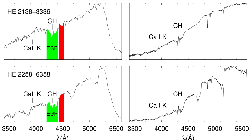
Figure 1.— Comparison between the low-resolution HES spectra (left panels) and GEMINI medium-resolution spectra (right panels). The green and red bands show, respectively, the line band and side band of the EGP index, defined by Placco et al. (2011).

Figure 1 shows a comparison between the low-resolution HES and the medium-resolution GMOS spectra of our stars. Even at low resolution, the CH G-band is clearly seen, and its strength is captured by the EGP index. In addition, these stars exhibit a weak Ca ii K line, indicating low metallicity. The medium-resolution GMOS spectra are of sufficient quality to determine estimates of the stellar parameters for the observed stars (see Section 3.1 for further details), and to determine the metallicity and carbon abundance ratio.

2.2. High-Resolution Spectroscopy

The final observational step was to obtain high-resolution spectroscopy of the most promising targets based on the results of the medium-resolution spectral analysis. These data were gathered using the MIKE instrument (Bernstein et al., 2003) on the Magellan-Clay Telescope at Las Campanas Observatory. We used the 0$\farcs$7 slit with 2$\times$2 on-chip binning, yielding a nominal resolving power of R $\sim 35,000$ in the blue and $\sim 28,000$ in the red region, with an average S/N $\sim 85$ at 5200 Å. MIKE spectra have nearly full optical wavelength coverage from $\sim$3500-9000 Å. Table 1 lists the details of the high-resolution observations for each star. These data were reduced using a data reduction pipeline developed for MIKE spectra.

3. Stellar Parameters

The stellar parameters ($T_{\rm eff}$ , log $g$ , [Fe/H]) were estimated first from the medium-resolution spectra, using the procedures described below. These values were used as first estimates for the determinations based on the high-resolution spectra.

3.1. Stellar Parameters from Medium-Resolution Spectra

Stellar parameters were determined using the n-SSPP, a modified version of the SEGUE Stellar Parameter Pipeline (SSPP; see Lee et al., 2008a, b; Allende Prieto et al., 2008; Lee et al., 2011; Smolinski et al., 2011, for a detailed description of the procedures used). The n-SSPP is a collection of routines for the analysis of non-SDSS/SEGUE data that employs both spectroscopic and photometric ($B_{0}$, $(B-V)_{0}$, $(U-B)_{0}$, $J_{0}$ and $(J-K)_{0}$) information as inputs, to make a series of estimates for each stellar parameter. Then, using $\chi^{2}$ minimization in dense grids of synthetic spectra, and averaging with other techniques as available, the best set of values is adopted. The internal errors for the stellar parameters are: 125 $K$ for $T_{\rm eff}$ , 0.25 dex for log $g$ , and 0.20 dex for [Fe/H]. External errors are of a similar size.

3.2. Stellar Parameters from MIKE Spectra

The determination of stellar physical parameters from high-resolution spectroscopy relies on the behavior of the abundances of individual absorption lines as a function of: (i) the excitation potential, $\chi$, of the lines from which the abundances are derived (effective temperature); (ii) the balance between two ionization stages of the same element (surface gravity) and; (iii) the reduced equivalent width of the lines measured (microturbulent velocity). The adopted parameters are the ones that minimize the trend between the line abundances, derived from the equivalent width of the atomic Fe I absorption lines, and the quantities (i), (ii), and (iii). Generally, elemental abundances are obtained by analysis of both equivalent widths and spectral synthesis. Equivalent widths are obtained by fitting Gaussian profiles to the observed atomic lines. For this purpose, we used a line list based on the compilation of Roederer et al. (2010b), as well as data retrieved from the VALD database (Kupka et al., 1999). Table 3 shows the lines used in this work, with their measured equivalent widths and abundances.

Figure 2.— Fe I abundances as a function of the excitation potential (left panels), and the reduced equivalent width (right panels). The solid lines mark the average abundance and the dashed lines represent linear functions fitted to the data. No clear trends exist, indicating well-determined estimates of the effective temperature, $T_{eff}$, and microtubulent velocity, $\xi$.

As seen in Figure 2 (left panels), over the range in $\chi$ from 0.0 to $\sim 4.5$ eV, the adopted temperatures ($T_{eff}=$ 5850 K for HE 2138$-$3336 and $T_{eff}=$ 4900 K for HE 2258$-$6358) do not present any significant trend of Fe I abundances. Likewise, the right panels of Figure 2 show no trends on the behavior of the derived Fe I abundances as a function of the reduced equivalent width, indicating appropriate values for the microturbulent velocity. The same applies for estimates of log $g$ , since the average values of Fe I and Fe II agree within to within 0.02 dex for both of our stars.

The final stellar parameters, from both medium- and high-resolution analysis, are summarized in Table 2. The uncertainties for the medium-resolution parameters were taken from the n-SSPP, and the uncertainties for the high-resolution determinations are discussed in detail in Section 4.6. It is worth noting the good agreement between the [Fe/H] and $T_{\rm eff}$  values for the medium- and high-resolution spectra. Differences in the log $g$  values arise mainly due to the difficulty of making this estimate from the medium-resolution spectra, in particular in the presence of strong carbon features. The derived effective temperatures and surface gravities from the high-resolution analysis are shown in Figure 3, compared with 12 Gyr Yale-Yonsei Isochrones (Demarque et al., 2004) for [Fe/H]=$-$3.0, $-$2.5, and $-$2.0.

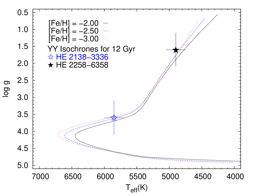
Figure 3.— The program stars shown in an H-R-Diagram, based on the stellar parameters determined from the high-resolution spectra (see Table 2). Overplotted are the Yale-Yonsei isochrones (Demarque et al., 2004), for ages of 12 Gyr and three different values of [Fe/H].

4. Abundance Analysis

Abundances for individual lines, derived from equivalent widths as well as from spectral synthesis of some features, are shown in Table 3. Line abundances obtained through spectral synthesis are marked with syn on the equivalent width column. Our chemical abundances (or upper limits) for 34 elements, derived from the MIKE spectra, are presented in Table 4. A description of our abundance analysis is given below.

4.1. Techniques

Our abundance analysis utilizes one-dimensional plane-parallel Kurucz model atmospheres with no overshooting (Castelli & Kurucz, 2004). They are computed under the assumption of local thermodynamic equilibrium (LTE). We use the 2011 version of the MOOG synthesis code (Sneden, 1973) for this analysis. Scattering in this MOOG version is treated with the implementation of a source function that sums both absorption and scattering components, rather than treating continuous scattering as true absorption (see Sobeck et al., 2011, for further details).

Our final abundance ratios, [X/Fe], are given with respect to the solar abundances of Asplund et al. (2009). Upper limits for elements for which no absorption lines were detected provide additional information for the interpretation of the overall abundance pattern of the stars. Based on the S/N ratio in the spectral region of the line, and employing the formula given in Frebel et al. (2006b), we derive 3 $\sigma$ upper limits for a few elements. All our abundances have been derived with LTE models, and where appropriate non-LTE corrections were applied A summary of the elemental abundances for our targets is given in Table 4.

4.2. Carbon, Nitrogen, and Oxygen

Carbon abundances were derived from both CH ($\lambda$4228 Å, $\lambda$4230 Å, and $\lambda$4250 Å) and C₂ ($\lambda$4737 Å, $\lambda$5165 Å, and $\lambda$5635 Å) molecular features. Figure 4 shows the C₂ band and the Mg I triplet for both targets, compared with the spectrum of HD 140283 ([Fe/H]=$-$2.2, $T_{\rm eff}$ =5725 K; Sobeck et al., 2007). In carbon-rich stars, continuum placement is a large source of uncertainty, since the many strong carbon features compromise its accurate determination. Figure 5 shows two of the features used for the carbon-abundance determinations for HE 2138$-$3336 and HE 2258$-$6358. CH $A-X$ band features are detected between 4240 Å and 4330 Å in HE 2138$-$3336, but were saturated for the cooler HE 2258$-$6358. As seen in Table 3, abundances derived from CH and C₂ features are in good agreement for both stars, with average values of [C/Fe]=$+$2.43 for HE 2138$-$3336 and [C/Fe]=$+$2.42 for HE 2258$-$6358.

Figure 4.— Examples of the spectral region around the C₂ molecular band at 5165 Å in our stars, compared with HD 140283. Also shown is the Mg I triplet.

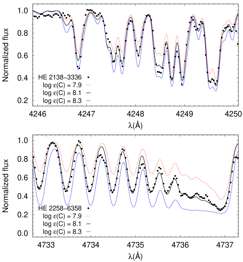
Figure 5.— Example of a CH band used for carbon-abundance determination for HE 2138$-$3336 (upper panel), and a C₂ band for HE 2258$-$6358. The dots represent the observed spectra, the solid line is the best abundance fit, and the dotted and dashed line are the lower and upper abundance limits, used to estimate the uncertainty.

Nitrogen abundances were determined from spectral synthesis of the CN band at $\lambda$3883 Å. For this purpose we used a fixed carbon abundance, based on the average of the individual abundances determined. Figure 6 shows the spectral synthesis for this region for both targets. In the case of HE 2138$-$3336, the observed spectra agrees well with the synthetic spectra within 0.2 dex. For HE 2258$-$6358, the band head appears to be saturated. Even so, it is possible to obtain an estimate of the nitrogen abundance to within 0.4 dex.

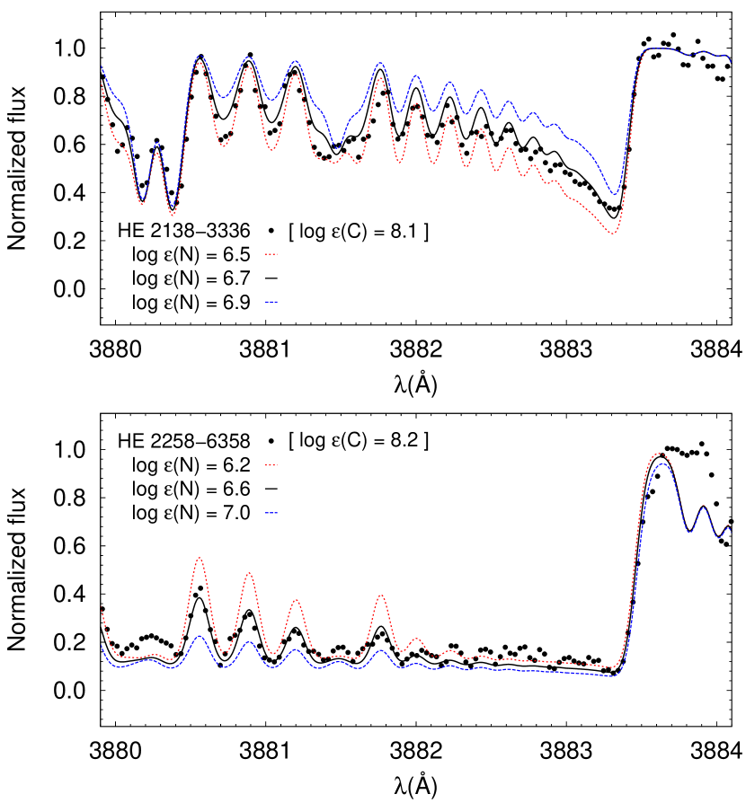
Figure 6.— Spectral synthesis of the CN band for nitrogen abundance determination. The dots represent the observed spectra, the solid line is the best abundance fit, and the dotted and dashed line are the lower and upper abundance limits, used to estimate the uncertainty.

The ¹²C/¹³C isotopic ratio is a sensitive indicator of the extent of mixing processes in cool red-giant stars. The comparison between the observed and synthetic spectra used for the determination of the ¹²C/¹³C isotopic ratio is shown in Figure 7. Using a fixed elemental carbon abundance, derived from the molecular features mentioned above, spectra employing three different values of ¹²C/¹³C = 19, 10, and 4 were compared to CH features around 4200 Å.

We find that a ratio of about 10 agrees well with the observed spectra for both HE 2138$-$3336 and HE 2258$-$6358. This ratio is consistent with other metal-poor CEMP stars (Sivarani et al., 2006) but is difficult to explain with current stellar evolutionary models, which predict much higher ratios for ¹²C/¹³C (e.g., see yields in Karakas, 2010a; Lugaro et al., 2012). The low ¹²C/¹³C ratios suggest substantial processing of ¹²C into ¹³C, where ¹²C is accreted from the donor AGB star and is the dominant isotope produced in the He-burning shells of the AGB stars. The mechanism for the processing in the donor star is unknown, although rotational mixing (Lagarde et al., 2012) and/or thermohaline mixing (Eggleton et al., 2008; Charbonnel & Zahn, 2007; Stancliffe, 2009, 2010), gravity waves (Denissenkov & Tout, 2000), and magnetic fields (Nordhaus et al., 2008; Busso et al., 2007; Palmerini et al., 2009) have been proposed as potential candidates.

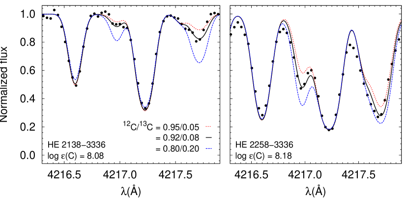
Figure 7.— Determination of the carbon isotopic ratio ¹²C/¹³C of our targets. The dots represent the observed spectra, the solid line is the best abundance fit, and the dotted and dashed line are the lower and upper abundance limits, used to estimate the uncertainty.

Figure 8 shows the distribution of the carbon and nitrogen (upper panels) and oxygen (lower panels) abundances for our stars, compared with literature data collected by Frebel (2010). The oxygen abundance for HE 2258$-$6358 was determined from the equivalent width of the $\lambda$6300 Å) forbidden line. For HE 2138$-$3336 , no usable oxygen lines were detected. The carbon and nitrogen abundances in Figure 8 are in agreement with other stars in the CEMP regime, and the oxygen abundance for HE 2258$-$6358 is also among typical values for CEMP stars in the literature. Interestingly, when comparing the behavior of the [C/O] ratio as a function of the carbon abundance for CEMP stars with [Ba/Fe] $\geq$ 0.0 (CEMP-s) and [Ba/Fe] $<$ 0.0 (CEMP-no), one finds that all stars with [C/O] $>$ 0.0 are classified as CEMP-s.

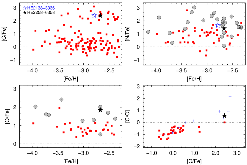
Figure 8.— Carbon abundances, as a function of the metallicity (upper panel), for the observed targets, shown as open and filled stars, and for literature determinations. The lower panels show [O/Fe] vs. [Fe/H]  and [C/O] vs. [C/Fe]  for HE 2258$-$6358. Filled squares are data collected by Frebel (2010) ([Fe/H]$<-$2.3), filled circles represent stars from the same database with [C/Fe]$>+$1.0, and blue crosses show stars with [Ba/Fe] $>+$1.0.

4.3. From Na to Zn

Abundances for Na, Mg, Al, Si, Ca, Sc, Ti, Cr, Mn, Co, and Ni were determined from equivalent width analysis for both stars, with the exception of Al and Si for HE 2258$-$6358. For Zn, only upper limits could be determined. Figure 9 shows the distribution of the light- element abundances as a function of metallicity, compared to literature data (Frebel, 2010). There is no significant difference in the behavior of the stars from this work and other CEMP stars in this metallicity range (filled gray circles). This is expected, assuming the gas which gave birth to the stars was preferentially enriched by massive SNII (Woosley & Weaver, 1995), in addition to the latter pollution by AGB companions.

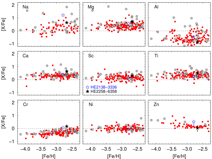
Figure 9.— Abundance ratios, [X/Fe], as a function of metallicity, for selected elements from Na to Zn. Filled squares are data collected by Frebel (2010) ([Fe/H]$<-$2.3), and filled circles represent stars from the same database with [C/Fe]$>+$1.0.

4.4. Neutron-Capture Elements

The chemical abundances for the neutron-capture elements were determined via spectral synthesis. Figure 10 shows the spectra of our two stars around the $\lambda$4554 Å Ba line, in comparison with HD 140283. The synthesis of neutron-capture absorption lines in the blue spectral region, particularly those close to molecular carbon features, were often hampered by the strong CH or CN features, and had to be excluded from the analysis. The results of the abundance determinations for individual elements and comments on specific features are given below.

Figure 10.— Examples of the spectral region around the Ba $\lambda$4554 Å line, compared with HD 140283.

Strontium, Yttrium, Zirconium

These three elements belong to the first peak of the $s$-process. Their abundances are mostly determined from absorption lines in blue spectral regions, which are affected by the presence of carbon features. The Sr $\lambda$4077 Å and $\lambda$4215 Å lines were saturated in the spectrum of HE 2258$-$6358, so the abundance was determined from the $\lambda$4607 Å line. Three Y lines were found at $\lambda>4800$ Å for HE 2258$-$6358, but were not detectable for HE 2138$-$3336, which had its Y abundance derived from the $\lambda$3774 Å line. Only one Zr line ($\lambda$4050 Å for HE 2258$-$6358  and $\lambda$4208 Å for HE 2138$-$3336) could be synthesized for each star. Other Zr features were either too weak or embedded in carbon molecular bands. The final [X/Fe] ratios for Sr, Y, and Zr are slightly overabundant ($>$ +0.3) in both stars, with respect to the solar values.

Barium, Lanthanum

These elements are representative of the second peak of the $s$-process. Ba is strongly overabundant in both stars. Figure 11 shows the spectral synthesis for the $\lambda$6496 Å line. Besides the $\lambda$4554 Å and $\lambda$4934 Å features (saturated for HE 2258$-$6358), additional abundances were calculated using the $\lambda$5853 Å and $\lambda$6141 Ålines. Final abundances are [Ba/Fe]$=$ +1.91 for HE 2138$-$3336  and [Ba/Fe]$=$ +2.23 for HE 2258$-$6358. Lanthanum is also overabundant in both stars; [La/Fe]$=$ +1.60 for HE 2138$-$3336  and [La/Fe]$=$ +1.91 for HE 2258$-$6358. There are a number of lines ranging from 4000-6000 Å suitable for spectral synthesis. Three lines ($\lambda$3995 Å, $\lambda$4086 Å, and $\lambda$4123 Å) were fitted with the same abundances for HE 2138$-$3336. Five other features were synthesized for HE 2258$-$6358, and the values determined from these lines agree within 0.1 dex.

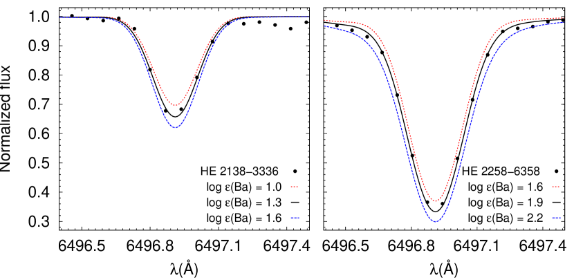
Figure 11.— Spectral synthesis for the $\lambda$6496 Å Ba line for HE 2138$-$3336  and HE 2258$-$6358. The dots represent the observed spectra, the solid line is the best abundance fit, and the dotted and dashed line are the lower and upper abundance limits, used to estimate the uncertainty.

Cerium, Praseodymium, Neodymium, Samarium

With the exception of Pr for HE 2138$-$3336, atomic lines for these species were found in the high-resolution spectra. Cerium and Sm abundances were determined from lines with $\lambda<4600$ Å. Even with many lines available for synthesis, most were weak and blended with carbon features. Only two Nd features could be synthesized for HE 2138$-$3336, while 9 suitable lines were found for HE 2258$-$6358. Figure 12 shows, on the right panels, the spectral synthesis for the $\lambda$4061 Å Nd line.

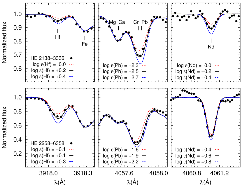
Figure 12.— Spectral synthesis of selected neutron-capture elements. The dots represent the observed spectra, the solid line is the best abundance fit, and the dotted and dashed line are the lower and upper abundance limits, used to estimate the uncertainty.

Europium

Eu is a well known indicator of $r$-process nucleosynthesis, and its abundance helps distinguish the r-only, r/s and s-only abundance regimes for CEMP stars. There are three lines ($\lambda$3724 Å, $\lambda$3907 Å and $\lambda$6645 Å) with abundances in reasonable agreement for HE 2258$-$6358  (average [Eu/Fe]= +1.68). In the case of HE 2138$-$3336, only an upper limit could be determined ([Eu/Fe]$<$ +1.09), based on the $\lambda$4129 Å and $\lambda$4205 Å features.

Gadolinium, Terbium, Dysprosium, Erbium

Abundances for these lanthanoids could only be determined for HE 2258$-$6358, and all features used have $\lambda<4200$ Å. One Tb feature was found at $\lambda$3702 Å, while at least two were found for Gd, Dy and Er, with the individual line abundances agreeing within 0.2 dex.

Thulium, Ytterbium, Hafnium, Osmium

This set of elements has many suitable features for spectral synthesis at $\lambda<4200$ Å. No Yb lines were found for HE 2258$-$6358, while one feature at $\lambda$3694 Å was found for HE 2138$-$3336. Figure 12 shows the spectral synthesis for the $\lambda$3918 Å Hf line (left panels).

Lead

This third-peak element is expected to be largely produced by the $s$-process (Travaglio et al., 2001). Abundances were determined using two features, $\lambda$3683 Å and $\lambda$4057 Å. For each star, these two lines yielded the same abundances values ([Pb/Fe] = +3.54 for HE 2138$-$3336 and [Pb/Fe] = +2.82 for HE 2258$-$6358). Figure 12 shows the spectral synthesis for the $\lambda$4057 Å line (middle panel). If the Pb abundance is determined from its neutral species (there are only neutral species available in the spectrum), than the abundance is strongly affected by non-local thermodynamic equilibrium (NLTE) effects. Hence, we adopt positive corrections for Pb abundances of 0.3 dex for HE 2138$-$3336 ([Pb/Fe] = +3.84) and 0.5 dex for HE 2258$-$6358 ([Pb/Fe] = +3.32), following Mashonkina et al. (2012). We also searched for possible NLTE corrections for other neutron-capture elements, such as Sr, Ba (Andrievsky et al., 2011; Bergemann et al., 2012) and Eu (Mashonkina et al., 2012). However, these measurements are based on ionized species (e.g. Sr II, Ba II, Eu II). In those cases, NLTE effects are expected to be much smaller than the effects found for neutral species. Indeed, in all cases, the corrections did not exceed the quoted uncertainties (0.07-0.15 $dex$) of the abundances, so no corrections were applied.

4.5. Comparisons with Other Very Metal-Poor Stars

Figure 13 shows the distribution of the abundances of selected neutron-capture elements for our program stars as a function of the metallicity, and compared to the literature data. Upper limits on abundances were excluded, and the stars with [C/Fe]$>+$1.0 are marked as filled circles. No significant differences are found between the abundances of our targets and the values from literature CEMP-s stars, for the elements of the first $s$-process peak (Sr, Y, and Zr), as well as between the second $s$-process (Ba and La) and $r$-process (Eu) peaks and literature values.

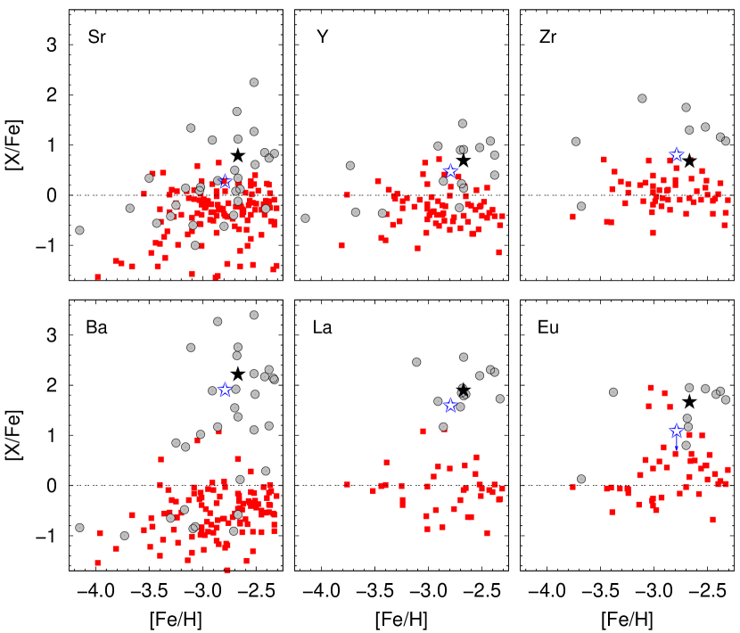
Figure 13.— Abundance ratios, [X/Fe], as a function of metallicity, for selected neutron-capture elements. Filled squares are data collected by Frebel (2010) ([Fe/H]$<-$2.3), and filled circles represent stars from the same database with [C/Fe]$>+$1.0.

The differences in the behavior of the abundances of elements formed by the $s$-process and $r$-process are useful to place constraints on possible formation scenarios for CEMP stars. Figure 14 presents a [Ba/Fe] vs. [Eu/Fe] diagram for the stars with [Fe/H]$<-$ 2.3 from the literature. Both targets from this work lie in the same location as other CEMP stars (filled circles). HE 2258$-$6358  is close to the limit set for the r/s regime, while the Eu upper limit for HE 2138$-$3336  places it in the s-only regime. More details are provided in Section 5.2.

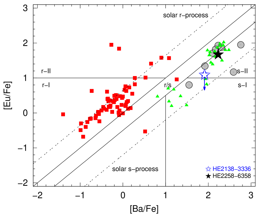
Figure 14.— [Eu/Fe] vs. [Ba/Fe] for the observed targets, compared with other neutron-capture-element enhanced stars. The solid lines represent the limits for the CEMP  classes defined by Beers & Christlieb (2005), and the dashed lines represent the solar $s$-process and $r$-process predictions for the [Ba/Eu] ratio, based on the fractions of Burris et al. (2000). Filled squares are data collected by Frebel (2010) ([Fe/H]$<-$2.3), filled circles represent stars from the same database with [C/Fe]$>+$1.0, and filled triangles are data from the CEMP stars listed in Table 6 (See Section 5.2 for more details).

At low metallicity, the $s$-process produces large amounts of Pb, and high [Pb/Fe] or [Pb/Eu] ratios are observational signatures of the $s$-process operating in metal-poor stars. Based on models of $s$-process nucleosynthesis in intermediate-mass stars on the AGB, the minimum $s$-process ratios predicted ([Pb/Eu] = +0.3) can be used to set a lower limit on the operation of the $s$-process (Roederer et al., 2010a).

Figure 15 shows the [Pb/Fe] (left panel) and [Pb/Eu] (right panel) ratios of our targets as a function of metallicity. Also shown are the NLTE corrections explained above. The lead abundances are within the range presented by other CEMP-s stars. Notably, the value for HE 2138$-$3336 ([Pb/Fe]= +3.54; +3.84 with NLTE correction) is the highest found to date in metal-poor stars. Also, the [Pb/Eu] ratio for both targets ([Pb/Eu] $=$ +2.45 for HE 2138$-$3336 and [Pb/Eu] = +1.14 for HE 2258$-$6358) are consistent with the limit set by Roederer et al. (2010a), which indicates that the Pb abundances for these stars come from the $s$-process nucleosynthesis that occured in their AGB companions.

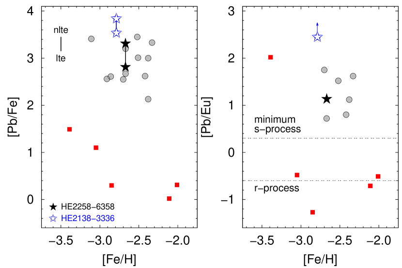
Figure 15.— [Pb/Fe] abundance (left panel) and [Pb/Eu] ratio (right panel) for the observed tagets. Filled squares are data from Cowan et al. (2002); Hill et al. (2002); Sneden et al. (2003); Masseron et al. (2006); Ivans et al. (2006), and filled circles represent stars with [C/Fe]$>+$1.0 from Aoki et al. (2002); Lucatello et al. (2003); Ivans et al. (2005); Barbuy et al. (2005); Cohen et al. (2006); Jonsell et al. (2006); Aoki et al. (2008). Dashed horizontal lines represent limits set by Roederer et al. (2010a).

4.6. Uncertainties

To determine the random uncertainties in our abundance estimates, we calculate the standard error of the individual line abundances for each ionization state of each element measured. For any abundance determined from equivalent-width measurements for less than 10 lines, we determined an appropriate small-sample adjustment for the standard error (Keeping, 1962). In the case of any abundance uncertainty that was calculated to be less than the uncertainty in the Fe I lines, we adopted the value from Fe I for that particular element. Typically, the Fe I standard error is $\sim 0.05$ dex.

For those lines with abundances determined via spectral synthesis, continuum placement is the greatest source of uncertainty, and it depends on the S/N of the region containing the particular line. Because of this, standard errors were determined with two procedures: (i) the uncertainty was taken directly from the spectral synthesis (e.g., Figure 12). Assuming a best value for the abundance of a given line, lower and upper abundance values were set so they would enclose the entire spectral feature; (ii) for the elements with two or more measured abundances, the uncertainties were calculated for small samples. For those elements with only one line, we adopt 0.1 dex as the minimum uncertainty for the abundance. Comparing the two values, the larger was taken as the standard error for the chemical abundances.

To obtain the systematic uncertainties in the abundance estimates, we redetermined abundances by individually varying the stellar parameters by their adopted uncertainties. We chose a nominal value of 150 K for the uncertainty in the effective temperature, as this value is similar to the random and systematic uncertainties in the determination of the atmospheric parameters. The same procedure was also applied for log $g$  (0.5 dex) and $\xi$ (0.3 km/s); results are shown in Table 5. Uncertainties in the effective temperature contribute the most to the abundance uncertainties. Uncertainties in the surface gravity are somewhat less important for the abundance determination of most species. For elements with particularly strong lines, especially those whose abundances are determined with spectral synthesis, the microturbulence can be an important source of uncertainty.

5. Abundance Patterns and Model Comparisons

Our overall aim is to compare the observed elemental abundances of our CEMP-s stars with the yields from AGB models. This way, constraints on the mass and metallicity of each progenitor can be obtained, allowing us to learn about the astrophysical sites of the first/early AGB nucleosynthesis events and the operation of the $s$-process.

In search of the progenitors of our observed neutron-capture elements a variety of stars or classes of stars could have been responsible. In general one first needs to distinguish whether the observed material was already present in the birth gas cloud or instead reflects a later-time external enrichment event. Our CEMP-s stars belong to the latter class, as their strong carbon overabundance in combination with neutron-capture overabundances associated with the s-process (as indicated by characteristic abundance ratios, such as Ba/Eu) are a tell-tale sign of a mass transfer event from a AGB star across a binary system.

The detailed study of such individual events (see below) greatly helps to piece together how the chemical evolution of neutron capture elements proceeded in the early universe. With few excpetions all metal-poor stars display some amount of neutron-capture elements in their surface which can be assumed to reflect the composition of their birth clouds. At the earliest times, these elements could have originated from massive, short-lived stars exploding as supernova. Presumably, some of these supernovae yielded neutron-capture elements made in the $r$-process. Next-generation stars then formed from r-process enriched gas. Indeed, most strongly r-process enhanced stars have a low metallicity of $\mbox{[Fe/H]}\sim-3.0$. In addition, massive stars that experience strong rotation could have also produced neutron-capture elements, but through the $s$-process elements. These stars would, however, produce $s$-process with a different distribution compared to low-mass AGB stars. Observations of “normal” metal-poor stars with $\mbox{[Fe/H]}\sim-3.0$ have help to disentangle these contributions from the different progenitors.

Later in the evolution of the Galaxy, lower-mass, longer-lived AGB stars began to dominate the production of neutron-capture elements, by producing $s$-process elements. Accordingly, metal-poor stars born after the onset of AGB enrichment formed from gas that was predominently enriched by the s-process. This evolution is somewhat reflected in the metallicities of metal-poor stars. Simmerer et al. (2004) suggests that the $s$-process may be fully active at [Fe/H]= $-$2.6, but this limit can be as low as [Fe/H]= $-$2.8, according to Sivarani et al. (2004) and in individual cases even lower. Furthermore, Roederer (2009) finds both pure $r$-process and pure $s$-process enrichment patterns extending over a wide metallicity range of $-3.0<$ [Fe/H] $<-0.4$.

Our target stars have [Fe/H]$>-$2.6 which canonically places them at a time when the general s-process production by AGB stars was already operating. However, in addition to that, our stars show the external s-process signature that allows us to reconstruct one of those s-process events occuring in AGB stars. We note here that models for the s-process in massive stars do not produce large amounts of Pb. Hence, massive stars cannot be responsible for the abundance patterns of our CEMP-s stars (e.g., see yields and discussion by Frischknecht et al., 2012).

We test this whole scenario by first comparing the observed abundances of our CEMP stars with the scaled Solar System $r$-process pattern (which is believed to be universal, according to e.g., Sneden et al., 2008). However, the abundances do not match this pattern, ruling out an $r$-process origin of the observed neutron-capture elements. We then compared the observed abundances with Solar System $s$-process predictions. The abundance do not match the $s$-process patten across for all elements, especially for the first-peak elements (Sr, Y, and Zr) as well as Pb. In particular, the model Pb abundances are underestimated by roughly 1.5 dex. This is not too surprising because we are working with old, metal-poor stars and the solar $s$-process pattern represents the integrated yields of AGB nucleosynthesis over billions of years up to the formation of the Sun. This natural disagreement, which is found for all CEMP-s and CEMP-r/s stars, is thought to occur because the $s$-process operates more efficiently at low metallicities. Owing to the high neutron-to-seed ratio, this leads to the production of a lot of Pb at early times in Galactic evolution (Gallino et al., 1998). Thus, a comparison of the observed abundances of our CEMP-s stars with $s$-process model predictions for low-metallicity AGB stars is required.

In this section we first present the results of new AGB models at the appropriate metallicities for our targets. Then, a detailed comparison between the yields of the models and the observed abundance patterns is presented for each star.

5.1. AGB Nucleosynthesis Models

If the observed metal-poor stars have been polluted from material from a previous AGB companion, then the observed abundances should reveal information about the efficiency of mixing events and chemical processing that took place during previous evolutionary phases, the mass-loss rate during the AGB phase, and the nature of the binary interaction that took place to pollute the observed star. Furthermore, non-standard mixing processes, such as thermohaline mixing, may act on the observed star and alter the accreted composition (e.g., Stancliffe & Glebbeek, 2008; Stancliffe, 2010). In light of this complex history, is it possible to explain the observed abundances using theoretical models of AGB stars?

Briefly, during the TP-AGB phase the He-burning shell becomes thermally unstable every $\approx 10^{5}$ years. The energy from the thermal pulse drives a convective pocket in the He-rich intershell, which mixes the products of He-nucleosynthesis within this region. The energy provided by the pulse expands the entire star, pushing the H-shell out to cooler regions where it is almost extinguished, and subsequently allowing the convective envelope to move inwards (in mass) to regions previously mixed by the flash-driven convective pocket. This inward movement of the convective envelope is known as the third dredge-up (TDU), and is responsible for enriching the surface in ¹²C and other products of He-burning, as well as heavy elements produced by the $s$-process. Following the TDU, the star contracts and the H-shell is re-ignited, providing most of the surface luminosity for the next interpulse period (see Busso et al., 1999; Herwig, 2005; Straniero et al., 2006, for reviews of AGB evolution and nucleosynthesis).

Details of the TDU phase are notoriously difficult to calculate in theoretical stellar evolution models (see e.g., Frost & Lattanzio, 1996; Mowlavi, 1999). Detailed stellar models suggest that the efficiency or depth of the TDU increases at low metallicity, which indicates that low-mass metal-poor AGB stars should be efficient producers of carbon and $s$-process elements (e.g., Karakas et al., 2002; Campbell & Lattanzio, 2008; Karakas, 2010a). Note that theoretical models of stars more massive than about 3$M_{\odot}$ at metallicities of [Fe/H] $\lesssim-2.3$ show the signature of hot bottom burning, when the convective envelope is subject to proton-capture nucleosynthesis via the CN cycle, leading to nitrogen-rich stars, where [N/C] $>+1$ (Johnson et al., 2007; Pols et al., 2012). Studies by Izzard et al. (2009), Bisterzo et al. (2012), and Lugaro et al. (2012) have indeed confirmed that many of the CEMP-s stars should exhibit the signature of low-mass AGB pollution, where the mass of the polluters is $1.2\lesssim M/M_{\odot}\lesssim 2.5$. Note that the latter two studies disagree on the origin of other types of CEMP stars, such as CEMP-r/s, which show enrichment by both the $r$- and $s$-process (see Beers & Christlieb, 2005, for definitions).

The derived elemental abundances for our newly-observed CEMP-s stars were compared with new predictions from a 1.3$M_{\odot}$ theoretical model with [Fe/H] = $-2.5$ (with a global metallicity of $Z=5\times 10^{-5}$). The AGB evolutionary model was calculated using the Mount Stromlo Stellar Evolutionary code (Karakas et al., 2010, and references therein), which uses the Vassiliadis & Wood (1993) mass-loss rate on the AGB, and a mixing-length parameter $\alpha=1.86$. The new AGB models presented here use updated molecular opacity tables compafred to those published in Karakas et al. (2010). We now use the C- and N-rich low temperature opacity tables from Marigo & Aringer (2009).

The model was evolved from the zero age main sequence, through the core helium flash and core helium burning, to the tip of the AGB. During the AGB, the model experienced 92 thermal pulses, and evolved to a final core mass of 0.82$M_{\odot}$. Out of those 92, 85 have experienced TDU episodes, with a total of 0.231$M_{\odot}$ of material dredged into the envelope. This large number of thermal pulses experiencing TDU is quite exceptional for a low-mass model, when for example the $M\approx 1.25M_{\odot}$ model of [Fe/H] $=-$2.3 presented in Karakas (2010b) only has 16 thermal pulses. Figure 16 shows the evolution of the radius with time for this new AGB model. The jump in the radius at $2.775\times 10^{9}$ years occurs after the first TDU event, which causes the star to become carbon rich, and consequently changes its internal structure. Note that the gap between thermal pulses shortens considerably.

Figure 16.— Evolution of the stellar radius as a function of time during the TP-AGB for the $1.3M_{\odot}$ AGB model presented in this section.

While the behavior of the new 1.3$M_{\odot}$ model during the AGB is unsual in that it reaches a high final core mass and experiences many thermal pulses, it is consistent and similar to other low-mass models of very low metallicity published in the literature. For example, the 0.9 or 1.0$M_{\odot}$ models of [Fe/H]$\approx-2.3$ (see discussions in Karakas, 2010a; Lugaro et al., 2012), end with relatively high final core masses ($M_{\rm core}>$ 0.7$M_{\odot}$). The 0.85$M_{\odot}$ model of $Z=0$ published by Campbell & Lattanzio (2008) also experiences a rapid rate of core growth (as discussed in detail in his PhD thesis; Campbell, 2007).

The final core mass is set by the competition between mass loss and core growth. The rate of core growth observed in the new 1.3$M_{\odot}$ model is rapid toward the end of the AGB. This is because the H-shell temperature is a function of the chemical composition and the core mass, and as the core mass increases so does the H-shell temperature and the rate of H-shell burning. A higher core growth rate in turn leads to a shortening of the interpulse phase, as the quicker build up of H-shell ashes leads to conditions suitable for a TP.

That the core is allowed to reach such high values is mostly as a result of the mass-loss rate used on the AGB. We use the Vassiliadis & Wood (1993) mass-loss prescription, which is a semi-empirical formula derived for stars with metallicities of the LMC, SMC, and Galaxy. That is, for stars with much higher Z than we are modeling and this adds a significant uncertainty into our calculations. The Vassiliadis & Wood (1993) formula depend on the radius, luminosity and mass so there is an implicit metallicity dependence included. The new 1.3$M_{\odot}$ model is more compact and consequently has a higher effective temperature (by 30%) compared to the 1.25$M_{\odot}$ model of [Fe/H]= $-2.3$. This is the reason for the large number of TPs. The model star lost a total of 0.50$M_{\odot}$ during the AGB (see Figure 17), which is only marginally smaller than the amount of mass lost by the 1.25$M_{\odot}$ of [Fe/H]= $-2.3$, which loses about 0.58$M_{\odot}$ (Karakas, 2010a). Furthermore, because the effective temperature never drops below 4,000 K that the effect of the updated low-temperature molecular opacity tables is minimal (e.g., Marigo, 2002).

Figure 17.— Evolution of the stellar radius as a function of mass (in units of $M_{\odot}$) during the TP-AGB for the $1.3M_{\odot}$ AGB model presented in this section.

One of the most significant uncertainties affecting the AGB lifetime of very low-metallicity AGB models is the interplay between the mass-loss rate and the surface composition. While these stars have very low iron abundances, the surface C abundance quickly reaches solar values after $\approx 10$ thermal pulses, owing to efficient TDU. There is observational evidence that carbon-enrichment leads to an increase in the mass-loss rate in cool evolved stars. For example, the near-infrared colors of carbon stars in the Magallanic Clouds are systematically redder than those of oxygen-rich stars (e.g., as seen in LMC surveys such as DENIS and 2MASS Cioni et al., 2000; Nikolaev & Weinberg, 2000). At the very low metallicities of the CEMP stars in the halo there are no direct observations of the mass-loss process in action. Instead, comparisons between CEMP stars and model predictions may provide some clues. Furthermore, it is possible that binary interactions terminate evolution along the AGB after the star becomes signficantly carbon rich. This could occur because carbon enrichment leads to an increase in the opacity, and hence an increase in the radius that causes the primary AGB star to overflow its Roche lobe.

The $s$-process abundance predictions were calculated using the post-processing nucleosynthesis code and full network of 320 species described in Lugaro et al. (2012), with reaction rates taken from the JINA REACLIB library (Cyburt et al., 2010). For the initial composition we used the solar distribution of abundances from Asplund et al. (2009), scaled down to [Fe/H] = $-$2.5. We use the same assumptions about the initial abundances as outlined in Alves-Brito et al. (2011). We did not consider an initial enhancement for the $\alpha$-elements. The inclusion of an initial enrichment of $\alpha$-elements does not affect the production of carbon or neutron-capture elements (e.g. Lugaro et al., 2012), which are the elements we used to determine a good fit between the model AGB star and the observed metal-poor stars. We also calculate one nucleosynthesis model where we scaled the iron abundance down to [Fe/H] = $-$2.8, using the stellar evolutionary sequence described above as input. This method is not entirely self-consistent, but it provides an indication of the $s$-process distribution expected at that metallicity (where a similar method is used by Bisterzo et al., 2010).

Low-mass AGB models of very low metallicity can also experience mild proton-ingestion episodes during the first few TPs and this can shape the initial s-process distribution (see discussion in Lugaro et al., 2012). We also find proton-ingestion in the 1.3$M_{\odot}$, [Fe/H] = $-2.5$ during the first TP but because the TDU does not begin until much later, the effect on the final s-process distribution and on the best fit to the CEMP star abundance distribution is minimal. Note that for the first $\approx 10$TPs, the ¹³C pockets burn under convective conditions (Regime 3 described in Lugaro et al., 2012).

While proton ingestion episodes are found with many evolution codes, the exact mass and metallicity range over which they occur is not agreed upon (compare the models of Campbell & Lattanzio, 2008; Lau et al., 2009; Suda & Fujimoto, 2010). The issue is further complicated by the fact that both evolutionary and nucleosynthetic predictions for these events may be inaccurate as there are many uncertainties associated with them. The development of hydrodynamical models for this phase of evolution (e.g. Herwig et al., 2011; Stancliffe et al., 2011) may eventually lead to an improvement in our understanding of such episodes.

In low-mass AGB stars the main neutron source is the ¹³C($\alpha$, n)¹⁶O reaction, which is activated in the He-intershell region between thermal pulses at temperatures of $T\gtrsim 90\times 10^{6}$K. Observational and theoretical evidence has shown that the ¹³C($\alpha$,n)¹⁶O reaction is the main neutron source in low-mass AGB stars of $\approx 1-3M_{\odot}$ (Gallino et al., 1998; Abia et al., 2002). In order to obtain an enrichment of $s$-process elements, we artificially introduce some protons into the top of the He-intershell region. This has become standard practice for such models, for the simple reason that there is insufficient ¹³C in the H-burning ashes of AGB stars to make it an efficient neutron source. We apply the assumption that the proton abundance in the intershell decreases monotonically from the envelope value of $\simeq$ 0.7 to a minimum value of 10^-4 at a given point in mass, located at “M_mix” below the base of the envelope (Goriely & Mowlavi, 2000). Protons are inserted at the deepest extent of each TDU episode, where the methodology is exactly the same as in e.g., Kamath et al. (2012) and Lugaro et al. (2012), which we refer to for a detailed discussion of the uncertainties. The mass of the proton profile is a free parameter, which we set to a constant mass of M${}_{\rm mix}=2\times 10^{-3}M_{\odot}$. The protons are captured by the abundant ¹²C in the He-intershell to form a ¹³C-rich region in the top 1/10^th of the intershell. Neutrons are then released by the ¹³C($\alpha$,n) ¹⁶O reaction during the interpulse period under mostly radiative conditions (Straniero et al., 1995).

5.2. Comparison with AGB Models

We compared the observed abundances of our CEMP stars with abundance predictions from the model described in Section 5.1 (1.3$M_{\odot}$ and $Z=5\times 10^{-5}$), as well as for 67 different AGB models from Karakas (2010a) and Lugaro et al. (2012). These models are in a range of masses of 0.9$M_{\odot}$ to 6.0$M_{\odot}$ and metallicity $Z=10^{-4}$, including models with $s$- and $r$-process enhancements in their initial abundance patterns prior to the AGB evolution. The data include yields for every thermal pulse of each model.

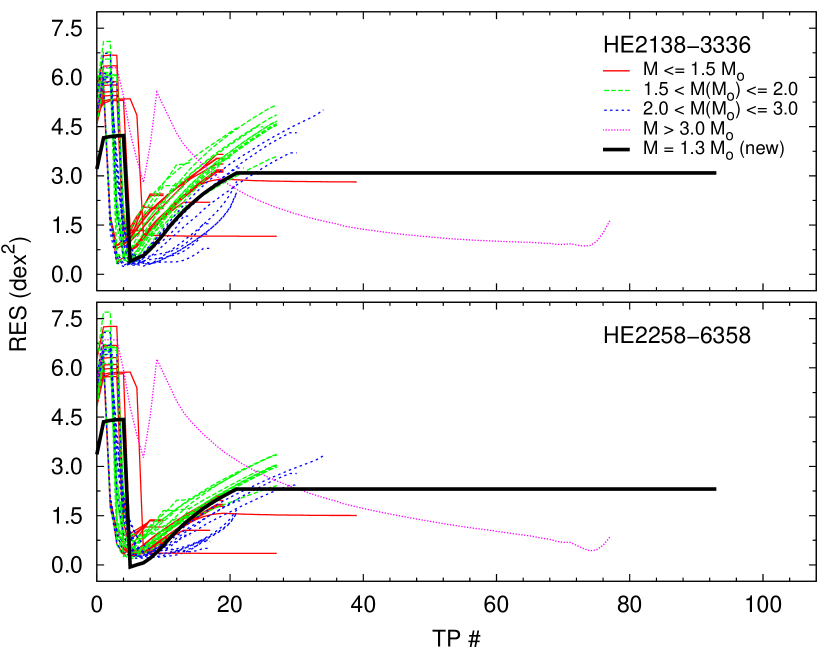
Figure 18.— Residual values of the model presented in Section 5.1, and other models from the literature, as a function of the thermal pulse number, TP#.

To identify the model (and thermal pulse) which best describes the observed abundances, a residual-like measurement was made. We took the sum of the squared differences between the abundances of each thermal pulse of a given model and the observed values, divided by the number of measured abundances, including all neutron-capture elements and carbon. Figure 18 shows the behavior of this quantity (RES), as a function of the thermal pulse number, for the model presented in this work (labeled $new$) and a series of models taken from the literature. With the exception of models with M $>3.0~{}M_{\odot}$, the lowest residual value is usually reached early in the evolution of the AGB star, for both HE 2138$-$3336 and HE 2258$-$6358.

Also in Figure 18 it is possible to note that, for HE 2258$-$6358, the lowest residual value is related to the new low-metallicity model described in Section 5.1. On the other hand, for HE 2138$-$3336, there seems to be a number of models with masses between 1.5$M_{\odot}$ and 3.0$M_{\odot}$ that yield lower residual values than the new model. Inspection of the individual abundances for each of these models reveals that the residuals are usually lowered by the good agreement for the elements between Ba and Eu. However, as stated above, those models fail to reproduce the abundances of the first s-process peak (Sr, Y, and Zr) and Pb.

The interpretation of the abundances in former mass-transfer systems is complicated by the fate of material accreted from the primary AGB star. Mass transfer is most likely to occur while the secondary is on the main sequence, but the secondary can have evolved substantially since then. If the star develops a deep convective envelope, the accreted material can become significantly diluted with pristine material from the stellar interior. The effect of dilution on the surface abundances will then be determined by the depth of the convective region and the mass of material that was accreted. The former can easily be supplied by stellar-evolution calculations, but we are forced to make some assumptions about the latter.

The above picture applies if convection is the only means by which accreted material can be mixed with the stellar interior. However, accreted material has undergone nuclear burning, and has a higher mean molecular weight than the pristine material of the secondary on which it now lies. This situation is unstable to the process of thermohaline mixing, and the accreted material can end up being mixed throughout a large portion of the secondary (see Stancliffe et al., 2007, for example). The extent of mixing depends upon the amount of accreted material and also on its composition. However, the depth to which thermohaline mixing reaches can be determined by a stellar-evolution code (Stancliffe & Glebbeek, 2008).

We note that, to calculate the residuals, our model abundances were not scaled to any of the observed abundance of each star. This procedure (scaling abundances to, e.g., Ba and Eu) is commonly used as an attempt to reproduce the relative $s$- and $r$-process contributions of each element to the observed abundance pattern, and cannot be used to quantitatively trace the enrichment episodes experienced by the object. On the contrary, the use of absolute abundances allows for an assessment of the effects of dilution across the binary system on the predicted abundance pattern. This can give clues to differences arising from the interaction between the AGB donor star and the receiving star.

We can compute the surface abundance of the secondary for a given element, $X$, using the equation:

$$X={M_{\mathrm{acc}}X_{\mathrm{acc}}+M_{\mathrm{i}}X_{\mathrm{i}}\over M_{\mathrm{mix}}},$$ (1)

where $M_{\mathrm{acc}}$ is the mass of material accreted, $M_{\mathrm{mix}}$ is the total mass over which material is mixed (inlcuding the accreted layer), $M_{\mathrm{i}}$ is the mass of pristine material which will become mixed (i.e., $M_{\mathrm{i}}=M_{\mathrm{mix}}-M_{\mathrm{acc}}$), and $X_{\mathrm{acc}}$ and $X_{\mathrm{i}}$ represent the accreted and initial compositions of the element. $M_{\mathrm{i}}$ can be determined from stellar models, and depends both on the evolutionary state of the object and the nature of the mixing mechanisms being considered.

Typical values for the quantities above were taken from Lugaro et al. (2008). We assume the masses of our metal-poor stars to be 0.8 M_⊙. When such a star is on its giant branch, its envelope reaches its maximum depth, so the outermost 60% of the star is convective. On the other hand, when the star is a subgiant/dwarf, this depth can be as low as 5%. The free parameters are $M_{acc}$, and the details of the AGB evolution, nucleosynthesis and mass transfer. Lugaro et al. (2008) find that, for their particular case, the currently observed fluorine-rich CEMP-s star should have accreted between 0.05 M_⊙ and 0.12 M_⊙ from its AGB companion, so a value of 0.10 M_⊙ was adopted in our case. In addition, the initial abundance pattern of the receiver star is taken to be the same as that of the donor prior to its AGB evolution, which is the solar distribution of abundances from Asplund et al. (2009), scaled down to [Fe/H]=$-$2.5.

It should be stressed that the assumption of 0.1 M_⊙ of accreted material may not be truly representative. The fluorine-rich star discussed in Lugaro et al. (2008) is an unusual object whose high level of fluorine enrichment requires a large mass of AGB ejecta to have been accreted (see also Stancliffe, 2009). In fact, the population synthesis modeling of Izzard et al. (2009) suggests that many systems accrete very little material. However, these models are based upon the use of a Bondi-Hoyle prescription for wind accretion, and a better treatment of the wind may lead to more accretion; it may be possible to accrete as much as 0.4 M_⊙ in exceptional circumstances (see Abate et al., 2013, for details).

In applying the above equation, we must take care that we correctly identify the depth of mixing. If we include only the action of convection, then when the star reaches the subgiant branch its convective envelope is not yet deep enough, and still lies within the accreted layer. No dilution of accreted material will have taken place so far. However, if thermohaline mixing is taken into account, accreted material will have mixed to a depth of around 0.5 M_⊙ from the surface (Stancliffe & Glebbeek, 2008). Thus, we distinguish two cases for HE 2138$-$3336  (log $g$ = 3.6): one with no dilution of accreted material, and one where we use $M_{\mathrm{mix}}=0.5$ and $M_{\mathrm{i}}=0.4$ in our dilution equation.

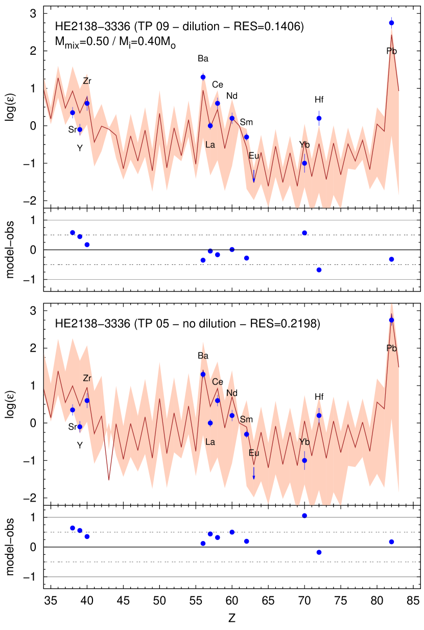
Figure 19.— Abundance pattern of HE 2138$-$3336, compared with the $M_{\mathrm{mix}}=0.5$ M_⊙ dilution case (top) and the non-dilution case (bottom). The model used is the one described in Section 5.1. The shaded area covers the model prediction ranges from the initial to the final abundances, and the solid line shows the abundance pattern for the thermal pulse having the lowest residual. The residual is calculated by the sum of the squared differences between the abundances of the thermal pulse and the observed values, divided by the number of measured abundances.

Figure 19 shows the abundance pattern of HE 2138$-$3336 in two cases. The top panel compares the observed abundances with the model described in Section 5.1, including dilution according to Equation 1; this case corresponds to the dilution of material by the action of thermohaline mixing. The lower panel shows the same comparison without dilution, i.e., for the case where only standard convection is considered. The shaded area covers the model prediction ranges from the initial to the final abundances, and the solid line shows the abundance pattern for the thermal pulse having the lowest residual. Indicated in each panel are the number of the best-matching thermal pulse and the value of the residual. It is worth noticing the agreement (within $\sim 2\sigma$) between the observed abundance pattern and the model including dilution. In this case, the values agree within around 0.5 dex, with the exception of Hf. For the model without dilution, nearly all the residuals are positive, suggesting an overproduction of all the heavy elements.

Figure 20 shows the residuals calculated for each thermal pulse, including dilution, compared with the residuals for the case without dilution included. For HE 2138$-$3336, the best residual is at TP#9 in the dilution case, whereas it is at TP#5 for the non-dilution case. The residual is significantly lower for the case with dilution.

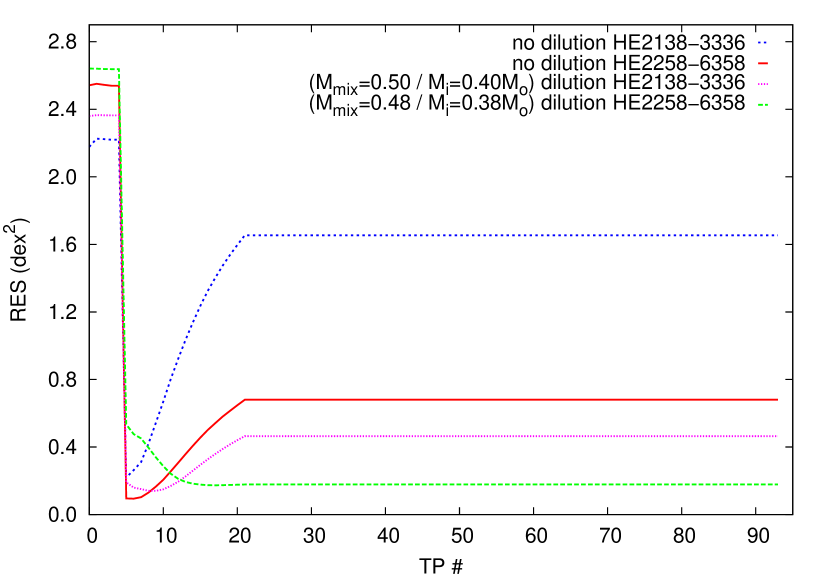
Figure 20.— Residual values, as a function of the thermal pulse number, for HE 2138$-$3336 and HE 2258$-$6358, with and without dilution.

The fact that our best fit, including dilution, happens at a relatively early pulse may point to the fact that the mass transfer in this system took place before the donor star was able to complete its full AGB evolution. Note that the AGB model used here enriches itself with carbon and s-elements between pulses 5 to 21. There are two possible reasons for the AGB star to transition to either a post-AGB star or directly into a white dwarf – either the mass transfer happened earlier as a result of binary interaction, or the mass-loss rates used in the model are not high enough. The fact that radial velocity variation is detected in this object may tentatively support the former hypothesis, as this suggests this system may be a close binary. However, we cannot rule out the possibility that the heavy element distribution could be better fit by a different mass of AGB donor, or if the s-process distribution is affected by uncertainties in the ¹³C pocket (see e.g. Bisterzo et al., 2010; Lugaro et al., 2012).

For the case of HE 2258-6358 (log $g=1.8$), the situation is somewhat simpler, because the star has undergone first dredge-up, which takes place between $2.3<\log g<3.2$ (e.g. Stancliffe et al., 2009). Any accreted material must have become mixed by convection at this point, even if it was unaffected by any other physical process while on the main sequence. The convective envelope reaches a depth of around 0.48 M_⊙. This is comparable to the depth of thermohaline mixing, so we can examine the two cases with a single calculation, namely $M_{\mathrm{mix}}=0.48M_{\odot}$, $M_{\mathrm{acc}}=0.1M_{\odot}$ and $M_{\mathrm{i}}=0.38M_{\odot}$.

The abundance pattern of HE 2258$-$6358 is shown in Figure 21. The best residual behavior occurs from TP#17 to the final abundance, assuming a mixing depth of $M_{\mathrm{mix}}=0.48$ M_⊙. However, in this case the residual value is worse than in the case of non-dilution (see Figure 20), with the non-dilution case having its best fit at TP#6. This result is problematic because HE 2258$-$6358  is a post-first dredge-up object. Any accreted material would have been mixed by the deepening of the convective envelope, if it had not previously been mixed by some other non-convective process. Although the dilution case yields higher residuals than the case with no dilution included, this behavior could be due to the possible r/s origin of HE 2258$-$6358, as seen in Figure 14. The observed values, especially for the elements from the second $r$-process peak, are consistently above the dilution model values. However, this does not apply for the Pb abundance, which is mainly formed by the $s$-process. This could be due to an underestimated initial abundances of the receiver star, which may have formed from a previously $r$-process enriched cloud. This previous enrichment could account for the differences between the observed abundances and the model values.

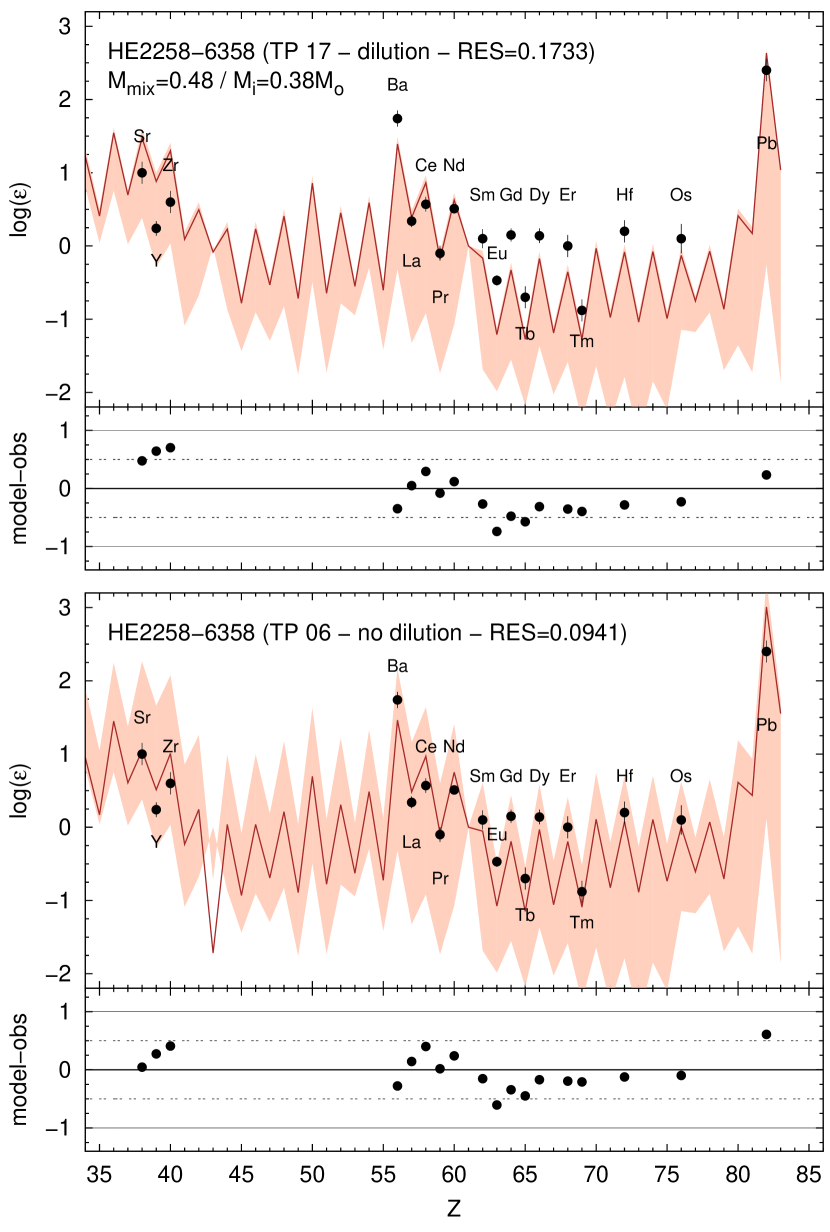
Figure 21.— Abundance pattern of HE 2258$-$6358, compared with the 60% depth dilution case (top) and the non-dilution case (bottom). The lines and symbols are the same as Figure 19.

Jonsell et al. (2006) lists several scenarios for CEMP-r/s production, including a binary system formed from an $r$-process-rich interstellar medium along with AGB pollution. They argue that the probability of forming a star from a pre-enriched $r$-process cloud, independent of AGB enrichment from a companion, is negligible, and suggest that the formation of the binary could be triggered by a supernova capable of producing $r$-process elements. In any case, in order to support this hypothesis, the nature of the binary (assuming it is such) for HE 2258$-$6358 must be determined by radial velocity monitoring.

To investigate this issue further, this analysis was extended to known CEMP-s and CEMP-r/s stars from the literature, and results are presented in Table 6. The stars selected have at least 7 abundances determined, including neutron-capture elements (up to 21 different species) and carbon. For the 26 stars in the table, the residuals were calculated for two cases: no dilution of accreted material, and the dilution over a mass range of 0.48 M_⊙ (corresponding to the case of dilution by either the convective envelope in the case of giants and by thermohaline mixing in the case of less evolved objects). The assumption of dilution does indeed present better residuals for log $g$ $<$ 2.5, while the no dilution case tends to give better fits in the case of objects with higher log $g$ . In the cases where no dilution gives the best fit, just over half the objects have their lowest residual at higher pulse numbers. For the dilution cases, three quarters of them have the their lowest residuals for pulse numbers of 10 or lower.

The reasons why low surface gravity objects can be fit by neutron-capture abundances of AGB stars having undergone few thermal pulses is not easy to explain. An early truncation of the AGB phase due to the presence of a companion should be rare, as few CEMP stars are found in close binary systems (Lucatello et al., 2003). In addition, the fate of the AGB donor should be independent of the present-day state of CEMP star, as mass transfer likely happened many gigayears ago. Clearly there is still further work needed in order to understand the nature of these systems. One note of caution should be added. We have only tried to fit the abundances from a single AGB star, and we have considered only one mass width for the partially-mixed zone that gives rise to the ¹³C pocket in the AGB nucleosynthesis calculation. It remains to be seen whether other choices of these parameters would result in improved fits.

Finally, by comparing the abundance patterns of HE 2258$-$6358 and the CEMP-r/s stars listed in Table 6 (green filled triangles in Figure 14), it is possible to note that all the CEMP-r/s analyzed show the same overproduction of the second peak $r$-process elements when compared with the AGB model presented in this work. This behavior is in agreement with recent studies (Bisterzo et al., 2012; Lugaro et al., 2012), which suggest that one possible scenario for the formation of the CEMP-r/s is a binary system formed in a molecular cloud pre-enriched with $r$-process elements. Moreover, 12 out of the 13 r/s stars in Table 6 present their lowest residual value for the non-dilution case, similar to the behavior of HE 2258$-$6358.

6. Conclusions

In this paper we have analyzed two newly-discovered CEMP stars, and compared their abundance patterns with yields from a low-mass, metal-poor AGB model, including the effects of dilution across a binary system.

Our targets were initially selected due to the presence of characteristic carbon-enhancement features in low- and medium-resolution spectra (Placco et al., 2010, 2011). The high-resolution follow-up spectra reported here allowed the determination of abundances (or upper limits) for 34 elements; light elements ($Z<30$) are in agreement with those of other typical halo stars, but their neutron-capture element abundances indicate these stars should be CEMP-s stars, enriched by the $s$-process. One of our targets, HE 2138$-$3336, exhibits a remarkably high Pb abundance ratio, supporting the hypothesis of relative lead overproduction in AGB stars at low metallicities. Both stars exhibit $s$-process signatures in their abundance patterns at metallicities [Fe/H]= $-$2.7 and $-$2.8, agreeing with statements that the onset of the s-process can be as early as [Fe/H]= $-$2.8 (Sivarani et al., 2004). We also confirm the CEMP-s classification of HE 2138$-$3336, through its abundance pattern and observed changes in radial velocity over the period of one year, and argue for the possible CEMP-r/s classification of HE 2258$-$6358, because no $s$-process model agrees well with the observed abundance pattern, likely due to a contribution of these elements by the $r$-process.

We compared our derived abundances with low-metallicity $s$-process models, assuming mass transfer across a binary system. We also took into account the effects of dilution in the binary system. The use of non-scaled abundances (e.g. with respect to Ba and Eu), when comparing the observations with yields from AGB models, opens a new opportunity for determining the characteristics of the progenitors of CEMP-s stars, allowing the study of dilution effects on the surface abundances of the AGB star. Extension of this analysis to other CEMP-s and CEMP-r/s stars found in the literature shows how complex the interaction in a binary system can be, and places constraints on the timescales and conditions which allow the mass transfer to take place, and generate the abundance pattern observed today.

Table 1Observationally Data for the Observed Candidates

	HE 2138$-$3336	HE 2258$-$6358
$\alpha$ (J2000)	21:41:20.4	23:01:48.6
$\delta$ (J2000)	$-$33:22:29.0	$-$63:42:24.0
V (mag)	15.0	14.5
(J$-$K)0	0.43	0.58
GPE ( Å)	41.7	56.9
EGP (mag)	$-$0.49	$-$0.28
Medium Resolution – Gemini/GMOS
Date	2011 07 20	2011 09 03
UT	08:25:40	07:03:49
Exptime (s)	800	960
vr(km/s)	63.9	103.6
High Resolution – Magellan/MIKE
Date	2011 11 03	2011 11 03
UT	02:55:33	00:44:53
Exptime (s)	3000	1800
vr(km/s)	56.1	102.1
S/N (4000 Å)	40	32
S/N (4500 Å)	58	47
S/N (5200 Å)	60	100
Date	2012 09 09	$\cdots$
UT	07:13:14	$\cdots$
Exptime (s)	860	$\cdots$
vr(km/s)	29.8	$\cdots$

Table 2 Derived Stellar Parameters

	Medium Resolution				High Resolution
	$T_{\rm eff}$ (K)	log $g$ (cgs)	[Fe/H]		$T_{\rm eff}$ (K)	log $g$ (cgs)	$\xi$(km/s)	[Fe/H]
HE 2138$-$3336	6036 (125)	2.62 (0.25)	$-$2.53 (0.20)		5850 (150)	3.60 (0.50)	1.60 (0.30)	$-$2.79 (0.01)
HE 2258$-$6358	4753 (125)	0.81 (0.25)	$-$2.94 (0.20)		4900 (150)	1.60 (0.50)	2.00 (0.30)	$-$2.67 (0.03)

Table 3 Equivalent Width Measurements

				HE 2138$-$3336		HE 2258$-$6358
Ion	$\lambda$	$\chi$	$\log\,gf$	$W$	$\log\epsilon$ (X)	$W$	$\log\epsilon$ (X)
	(Å)	(eV)		(mÅ)		(mÅ)
C CH	4228.00	$\cdots$	$\cdots$	syn	8.1	$\cdots$	$\cdots$
C CH	4230.00	$\cdots$	$\cdots$	syn	8.1	$\cdots$	$\cdots$
C CH	4250.00	$\cdots$	$\cdots$	syn	8.1	syn	8.0
C C2	4737.00	$\cdots$	$\cdots$	$\cdots$	$\cdots$	syn	8.1
C C2	5165.00	$\cdots$	$\cdots$	$\cdots$	$\cdots$	syn	8.4
C C2	5635.00	$\cdots$	$\cdots$	$\cdots$	$\cdots$	syn	8.2
N CN	3883.00	$\cdots$	$\cdots$	syn	6.7	syn	6.6
O I	6300.30	0.00	$-$9.82	$\cdots$	$\cdots$	32.4	7.9
Na I	5889.95	0.00	0.11	194.0	4.8	192.8	4.2
Na I	5895.92	0.00	$-$0.19	143.9	4.6	169.2	4.2
Mg I	4702.99	4.33	$-$0.38	49.2	5.3	$\cdots$	$\cdots$
Mg I	5172.68	2.71	$-$0.45	160.7	5.4	202.7	5.4
Mg I	5183.60	2.72	$-$0.24	$\cdots$	$\cdots$	326.7	5.9
Mg I	5528.40	4.34	$-$0.50	47.1	5.4	$\cdots$	$\cdots$
Al I	3961.52	0.01	$-$0.34	87.7	3.2	syn	2.9
Si I	4102.94	1.90	$-$3.14	$\cdots$	$\cdots$	syn	5.2
Ca I	4454.78	1.90	0.26	55.3	4.1	$\cdots$	$\cdots$
Ca I	5588.76	2.52	0.21	17.8	3.9	59.8	4.2
Ca I	5594.47	2.52	0.10	$\cdots$	$\cdots$	69.7	4.5
Ca I	6162.17	1.90	$-$0.09	35.8	4.0	89.1	4.3
Ca I	6439.07	2.52	0.47	21.8	3.8	$\cdots$	$\cdots$
Sc II	4246.82	0.32	0.24	syn	0.2	$\cdots$	$\cdots$
Sc II	5641.00	1.50	$-$1.13	$\cdots$	$\cdots$	10.9	0.8
Sc II	5657.91	1.51	$-$0.60	$\cdots$	$\cdots$	26.3	0.8
Ti I	5210.39	0.05	$-$0.83	$\cdots$	$\cdots$	61.5	3.0
Ti II	3759.29	0.61	0.28	98.5	2.3	$\cdots$	$\cdots$
Ti II	3913.46	1.12	$-$0.42	55.7	2.4	$\cdots$	$\cdots$
Ti II	4443.80	1.08	$-$0.72	43.7	2.3	$\cdots$	$\cdots$
Ti II	4468.52	1.13	$-$0.60	53.5	2.5	$\cdots$	$\cdots$
Ti II	4501.27	1.12	$-$0.77	36.8	2.3	$\cdots$	$\cdots$
Ti II	4533.96	1.24	$-$0.53	52.0	2.5	$\cdots$	$\cdots$
Ti II	4563.77	1.22	$-$0.96	37.1	2.6	$\cdots$	$\cdots$
Ti II	4571.97	1.57	$-$0.32	46.1	2.5	$\cdots$	$\cdots$
Ti II	5185.90	1.89	$-$1.49	$\cdots$	$\cdots$	38.7	2.7
Ti II	5226.54	1.57	$-$1.26	$\cdots$	$\cdots$	87.6	3.0
Ti II	5381.02	1.57	$-$1.92	$\cdots$	$\cdots$	43.1	2.9
Cr I	4254.33	0.00	$-$0.11	67.2	2.8	$\cdots$	$\cdots$
Cr I	5206.04	0.94	0.02	23.8	2.6	95.3	3.0
Cr I	5208.42	0.94	0.16	40.2	2.8	$\cdots$	$\cdots$
Cr I	5345.80	1.00	$-$0.95	$\cdots$	$\cdots$	53.0	3.3
Mn I	4030.75	0.00	$-$0.48	72.6	2.8	$\cdots$	$\cdots$
Mn I	4033.06	0.00	$-$0.62	49.8	2.4	$\cdots$	$\cdots$
Fe I	3565.38	0.96	$-$0.13	104.4	4.7	$\cdots$	$\cdots$
Fe I	3608.86	1.01	$-$0.09	104.3	4.7	$\cdots$	$\cdots$
Fe I	3727.62	0.96	$-$0.61	90.3	4.7	$\cdots$	$\cdots$
Fe I	3743.36	0.99	$-$0.79	85.6	4.7	$\cdots$	$\cdots$
Fe I	3753.61	2.18	$-$0.89	32.8	4.8	$\cdots$	$\cdots$
Fe I	3767.19	1.01	$-$0.39	103.1	4.8	$\cdots$	$\cdots$
Fe I	3786.68	1.01	$-$2.19	20.9	4.6	$\cdots$	$\cdots$
Fe I	3805.34	3.30	0.31	40.9	4.8	$\cdots$	$\cdots$
Fe I	3827.82	1.56	0.09	99.3	4.7	$\cdots$	$\cdots$
Fe I	3856.37	0.05	$-$1.28	103.2	4.7	$\cdots$	$\cdots$
Fe I	3902.95	1.56	$-$0.44	78.9	4.7	$\cdots$	$\cdots$
Fe I	3917.18	0.99	$-$2.15	31.5	4.8	$\cdots$	$\cdots$
Fe I	3940.88	0.96	$-$2.60	19.1	4.9	$\cdots$	$\cdots$
Fe I	4005.24	1.56	$-$0.58	75.2	4.7	$\cdots$	$\cdots$
Fe I	4014.53	3.05	$-$0.59	15.7	4.8	$\cdots$	$\cdots$
Fe I	4045.81	1.49	0.28	116.0	4.7	$\cdots$	$\cdots$
Fe I	4063.59	1.56	0.06	103.7	4.7	$\cdots$	$\cdots$
Fe I	4071.74	1.61	$-$0.01	94.0	4.7	$\cdots$	$\cdots$
Fe I	4132.06	1.61	$-$0.68	64.2	4.6	$\cdots$	$\cdots$
Fe I	4143.41	3.05	$-$0.20	33.0	4.9	$\cdots$	$\cdots$
Fe I	4143.87	1.56	$-$0.51	72.4	4.6	$\cdots$	$\cdots$
Fe I	4191.43	2.47	$-$0.67	33.5	4.8	$\cdots$	$\cdots$
Fe I	4202.03	1.49	$-$0.69	69.4	4.6	$\cdots$	$\cdots$
Fe I	4227.43	3.33	0.27	34.4	4.7	$\cdots$	$\cdots$
Fe I	4250.79	1.56	$-$0.71	69.3	4.7	$\cdots$	$\cdots$
Fe I	4260.47	2.40	0.08	71.2	4.7	$\cdots$	$\cdots$
Fe I	4404.75	1.56	$-$0.15	96.5	4.7	$\cdots$	$\cdots$
Fe I	4461.65	0.09	$-$3.19	28.1	4.8	$\cdots$	$\cdots$
Fe I	4466.55	2.83	$-$0.60	28.2	4.9	$\cdots$	$\cdots$
Fe I	4494.56	2.20	$-$1.14	24.4	4.8	$\cdots$	$\cdots$
Fe I	4528.61	2.18	$-$0.82	34.9	4.7	$\cdots$	$\cdots$
Fe I	4871.32	2.87	$-$0.36	26.8	4.7	$\cdots$	$\cdots$
Fe I	4872.14	2.88	$-$0.57	20.3	4.7	$\cdots$	$\cdots$
Fe I	4890.76	2.88	$-$0.39	32.1	4.8	$\cdots$	$\cdots$
Fe I	4891.49	2.85	$-$0.11	47.8	4.8	$\cdots$	$\cdots$
Fe I	4918.99	2.85	$-$0.34	24.4	4.6	$\cdots$	$\cdots$
Fe I	4920.50	2.83	0.07	42.7	4.5	$\cdots$	$\cdots$
Fe I	5166.28	0.00	$-$4.12	$\cdots$	$\cdots$	61.3	4.9
Fe I	5171.60	1.49	$-$1.72	34.4	4.8	92.6	4.8
Fe I	5192.34	3.00	$-$0.42	19.5	4.7	$\cdots$	$\cdots$
Fe I	5194.94	1.56	$-$2.02	$\cdots$	$\cdots$	75.4	4.9
Fe I	5198.71	2.22	$-$2.09	$\cdots$	$\cdots$	23.0	4.8
Fe I	5202.34	2.18	$-$1.87	$\cdots$	$\cdots$	52.4	5.0
Fe I	5216.27	1.61	$-$2.08	$\cdots$	$\cdots$	66.6	4.8
Fe I	5217.39	3.21	$-$1.16	$\cdots$	$\cdots$	31.0	5.1
Fe I	5232.94	2.94	$-$0.06	44.3	4.8	72.9	4.5
Fe I	5254.96	0.11	$-$4.76	$\cdots$	$\cdots$	21.4	4.9
Fe I	5266.56	3.00	$-$0.39	21.2	4.7	66.0	4.7
Fe I	5269.54	0.86	$-$1.33	81.7	4.8	153.5	4.9
Fe I	5281.79	3.04	$-$0.83	$\cdots$	$\cdots$	38.6	4.8
Fe I	5283.62	3.24	$-$0.52	$\cdots$	$\cdots$	50.3	4.9
Fe I	5324.18	3.21	$-$0.10	30.4	4.8	72.2	4.8
Fe I	5328.04	0.92	$-$1.47	64.6	4.6	128.8	4.7
Fe I	5328.53	1.56	$-$1.85	16.2	4.6	84.7	4.8
Fe I	5371.49	0.96	$-$1.64	61.8	4.8	142.9	5.2
Fe I	5397.13	0.92	$-$1.98	45.3	4.7	116.0	4.9
Fe I	5405.77	0.99	$-$1.85	47.4	4.7	100.4	4.5
Fe I	5415.20	4.39	0.64	$\cdots$	$\cdots$	43.0	4.9
Fe I	5429.70	0.96	$-$1.88	48.2	4.7	106.9	4.6
Fe I	5434.52	1.01	$-$2.13	28.1	4.6	$\cdots$	$\cdots$
Fe I	5446.92	0.99	$-$1.91	45.3	4.7	$\cdots$	$\cdots$
Fe I	5586.76	3.37	$-$0.14	21.7	4.8	57.9	4.8
Fe I	5615.64	3.33	0.05	21.2	4.5	$\cdots$	$\cdots$
Fe I	5658.82	3.40	$-$0.79	$\cdots$	$\cdots$	19.7	4.7
Fe I	6065.48	2.61	$-$1.41	$\cdots$	$\cdots$	30.0	4.6
Fe I	6136.61	2.45	$-$1.41	$\cdots$	$\cdots$	51.3	4.8
Fe I	6137.69	2.59	$-$1.35	$\cdots$	$\cdots$	44.7	4.8
Fe I	6219.28	2.20	$-$2.45	$\cdots$	$\cdots$	24.8	5.1
Fe I	6230.72	2.56	$-$1.28	$\cdots$	$\cdots$	43.8	4.7
Fe I	6252.56	2.40	$-$1.69	$\cdots$	$\cdots$	29.8	4.7
Fe I	6393.60	2.43	$-$1.58	$\cdots$	$\cdots$	57.2	5.0
Fe I	6400.00	3.60	$-$0.29	$\cdots$	$\cdots$	49.0	5.0
Fe I	6421.35	2.28	$-$2.01	$\cdots$	$\cdots$	28.8	4.8
Fe I	6430.85	2.18	$-$1.95	$\cdots$	$\cdots$	43.4	4.9
Fe I	6494.98	2.40	$-$1.24	$\cdots$	$\cdots$	60.3	4.7
Fe I	6677.99	2.69	$-$1.42	$\cdots$	$\cdots$	52.0	5.1
Fe II	4233.17	2.58	$-$1.97	35.8	4.8	$\cdots$	$\cdots$
Fe II	4522.63	2.84	$-$2.25	18.8	5.0	$\cdots$	$\cdots$
Fe II	4583.84	2.81	$-$1.93	18.2	4.6	$\cdots$	$\cdots$
Fe II	4923.93	2.89	$-$1.32	38.7	4.5	$\cdots$	$\cdots$
Fe II	5018.45	2.89	$-$1.22	50.6	4.7	$\cdots$	$\cdots$
Fe II	5234.63	3.22	$-$2.18	$\cdots$	$\cdots$	37.2	4.8
Fe II	5276.00	3.20	$-$2.01	$\cdots$	$\cdots$	49.3	4.9
Co I	3845.47	0.92	0.01	60.0	3.0	$\cdots$	$\cdots$
Co I	4121.32	0.92	$-$0.32	24.5	2.6	$\cdots$	$\cdots$
Ni I	3807.14	0.42	$-$1.22	47.7	3.3	$\cdots$	$\cdots$
Ni I	3858.30	0.42	$-$0.95	65.0	3.5	$\cdots$	$\cdots$
Zn I	4722.15	4.03	$-$0.39	6.5	2.5	$\cdots$	$\cdots$
Zn I	4810.53	4.08	$-$0.14	4.4	2.1	13.3	1.9
Sr II	4077.00	0.00	$-$1.26	syn	0.4	$\cdots$	$\cdots$
Sr II	4215.00	0.00	$-$1.32	syn	0.3	$\cdots$	$\cdots$
Sr II	4607.33	0.00	$-$0.57	$\cdots$	$\cdots$	syn	1.0
Y II	3774.33	0.13	0.21	syn	$-$0.1	$\cdots$	$\cdots$
Y II	4854.87	0.99	$-$0.38	$\cdots$	$\cdots$	syn	0.2
Y II	5200.41	0.99	$-$0.57	$\cdots$	$\cdots$	syn	0.2
Y II	5205.73	1.03	$-$0.34	$\cdots$	$\cdots$	syn	0.3
Zr II	4050.33	0.71	$-$1.00	$\cdots$	$\cdots$	syn	0.6
Zr II	4208.99	0.71	$-$0.46	syn	0.6	$\cdots$	$\cdots$
Ba II	4554.03	0.00	0.14	syn	1.3	$\cdots$	$\cdots$
Ba II	4934.10	0.00	$-$0.16	syn	1.4	$\cdots$	$\cdots$
Ba II	5853.68	0.60	$-$2.56	syn	1.3	syn	1.6
Ba II	6141.71	0.70	$-$0.08	syn	1.2	syn	1.7
Ba II	6496.91	0.60	$-$0.38	syn	1.3	syn	1.9
La II	3995.74	0.17	$-$0.06	syn	0.0	$\cdots$	$\cdots$
La II	4086.71	0.00	$-$0.07	syn	0.0	$\cdots$	$\cdots$
La II	4123.22	0.32	0.13	syn	0.0	$\cdots$	$\cdots$
La II	4526.12	0.77	$-$0.59	$\cdots$	$\cdots$	syn	0.3
La II	4921.79	0.24	$-$0.45	$\cdots$	$\cdots$	syn	0.3
La II	5290.84	0.00	$-$1.65	$\cdots$	$\cdots$	syn	0.3
La II	5303.53	0.32	$-$1.35	$\cdots$	$\cdots$	syn	0.4
La II	5797.57	0.24	$-$1.36	$\cdots$	$\cdots$	syn	0.4
Ce II	4053.50	0.00	$-$0.71	syn	0.7	$\cdots$	$\cdots$
Ce II	4083.22	0.70	0.27	syn	0.5	$\cdots$	$\cdots$
Ce II	4127.36	0.68	0.31	$\cdots$	$\cdots$	syn	0.5
Ce II	4222.64	0.79	$-$1.31	$\cdots$	$\cdots$	syn	0.5
Ce II	4562.36	0.48	0.23	syn	0.6	syn	0.7
Pr II	3964.82	0.06	0.12	$\cdots$	$\cdots$	syn	$-$0.3
Pr II	3965.26	0.20	0.14	$\cdots$	$\cdots$	syn	$-$0.1
Pr II	5220.01	0.79	0.30	$\cdots$	$\cdots$	syn	0.0
Pr II	5292.61	0.65	$-$0.26	$\cdots$	$\cdots$	syn	0.0
Nd II	4004.00	0.06	$-$0.57	$\cdots$	$\cdots$	syn	0.5
Nd II	4011.06	0.47	$-$0.76	$\cdots$	$\cdots$	syn	0.5
Nd II	4012.70	0.00	$-$0.60	$\cdots$	$\cdots$	syn	0.5
Nd II	4013.22	0.18	$-$1.10	$\cdots$	$\cdots$	syn	0.5
Nd II	4021.33	0.32	$-$0.10	syn	0.2	syn	0.3
Nd II	4043.59	0.32	$-$0.71	$\cdots$	$\cdots$	syn	0.5
Nd II	4061.08	0.47	0.55	syn	0.2	syn	0.6
Nd II	4069.26	0.06	$-$0.57	$\cdots$	$\cdots$	syn	0.6
Nd II	5249.58	0.97	0.20	$\cdots$	$\cdots$	syn	0.6
Sm II	4318.93	0.28	$-$0.25	syn	$-$0.3	$\cdots$	$\cdots$
Sm II	4434.32	0.38	$-$0.07	$\cdots$	$\cdots$	syn	0.0
Sm II	4467.34	0.66	0.15	syn	$-$0.3	$\cdots$	$\cdots$
Sm II	4499.48	0.25	$-$0.87	$\cdots$	$\cdots$	syn	0.2
Eu II	3724.93	0.00	$-$0.09	$\cdots$	$\cdots$	syn	$-$0.4
Eu II	3907.11	0.21	0.17	$\cdots$	$\cdots$	syn	$-$0.6
Eu II	4129.72	0.00	0.22	8.6	$-$1.1	$\cdots$	$\cdots$
Eu II	4205.04	0.00	0.21	6.5	$-$1.3	$\cdots$	$\cdots$
Eu II	6645.06	1.38	0.12	$\cdots$	$\cdots$	syn	$-$0.4
Gd II	3481.80	0.49	0.11	$\cdots$	$\cdots$	syn	0.1
Gd II	4251.73	0.38	$-$0.22	$\cdots$	$\cdots$	syn	0.2
Tb II	3702.85	0.13	0.44	$\cdots$	$\cdots$	syn	$-$0.7
Dy II	3445.57	0.00	$-$0.15	$\cdots$	$\cdots$	syn	0.2
Dy II	3531.71	0.00	0.77	$\cdots$	$\cdots$	syn	0.2
Dy II	4103.31	0.10	$-$0.38	$\cdots$	$\cdots$	syn	0.0
Er II	3729.52	0.00	$-$0.59	$\cdots$	$\cdots$	syn	0.0
Er II	3938.63	0.00	$-$0.52	$\cdots$	$\cdots$	syn	0.0
Tm II	3700.26	0.03	$-$0.38	$\cdots$	$\cdots$	syn	$-$0.9
Tm II	3701.36	0.00	$-$0.54	$\cdots$	$\cdots$	syn	$-$0.8
Yb II	3694.37	0.00	$-$0.30	syn	$-$1.0	$\cdots$	$\cdots$
Hf II	3918.08	0.45	$-$1.01	syn	0.2	syn	0.1
Hf II	4093.15	0.45	$-$1.15	$\cdots$	$\cdots$	syn	0.3
Os I	4260.80	0.00	$-$1.44	$\cdots$	$\cdots$	syn	0.1
Pb I	3683.46	0.97	$-$0.46	syn	2.5	syn	1.9
Pb I	4057.81	1.32	$-$0.17	syn	2.5	syn	1.9

Table 4 Abundances

			HE 2138$-$3336						HE 2258$-$6358
Element	Ion	$\log\epsilon$ (X)⊙	$\log\epsilon$ (X)	[X/H]	[X/Fe]	$\sigma$	$N_{\rm lines}$		$\log\epsilon$ (X)	[X/H]	[X/Fe]	$\sigma$	$N_{\rm lines}$
C	$\cdots$	8.43	8.08	$-$0.36	2.43	0.05	4		8.18	$-$0.25	2.42	0.09	4
N	$\cdots$	7.83	6.70	$-$1.13	1.66	0.20	1		6.60	$-$1.23	1.44	0.25	1
O	1	8.69	$\cdots$	$\cdots$	$\cdots$	$\cdots$	$\cdots$		7.87	$-$0.82	1.85	0.10	1
Na	1	6.24	4.67	$-$1.57	1.22	0.10	2		4.22	$-$2.02	0.65	0.10	2
Mg	1	7.60	5.38	$-$2.22	0.57	0.12	3		5.65	$-$1.95	0.72	0.30	2
Al	1	6.45	3.21	$-$3.24	$-$0.45	0.10	1		2.90	$-$3.55	$-$0.88	0.10	1
Si	1	7.51	$\cdots$	$\cdots$	$\cdots$	$\cdots$	$\cdots$		5.20	$-$2.31	0.38	0.10	1
Ca	1	6.34	3.94	$-$2.40	0.39	0.09	4		4.32	$-$2.02	0.65	0.09	3
Sc	2	3.15	1.23	$-$1.92	0.87	0.10	1		0.79	$-$2.36	0.31	0.05	2
Ti	1	4.95	$\cdots$	$\cdots$	$\cdots$	$\cdots$	$\cdots$		2.79	$-$2.16	0.51	0.10	1
Ti	2	4.95	2.40	$-$2.55	0.24	0.04	8		2.84	$-$2.11	0.56	0.08	3
Cr	1	5.64	2.76	$-$2.88	$-$0.09	0.07	3		3.14	$-$2.50	0.17	0.16	2
Mn	1	5.43	2.56	$-$2.87	$-$0.08	0.24	2		$\cdots$	$\cdots$	$\cdots$	$\cdots$	$\cdots$
Fe	1	7.50	4.71	$-$2.79	0.00	0.01	53		4.83	$-$2.67	0.00	0.03	35
Fe	2	7.50	4.71	$-$2.79	0.00	0.13	5		4.85	$-$2.65	0.02	0.03	2
Co	1	4.99	2.81	$-$2.18	0.61	0.29	2		$\cdots$	$\cdots$	$\cdots$	$\cdots$	$\cdots$
Ni	1	6.22	3.40	$-$2.82	$-$0.03	0.08	2		$\cdots$	$\cdots$	$\cdots$	$\cdots$	$\cdots$
Zn	1	4.56	2.30	$-$2.26	$<$0.53	$\cdots$	2		1.94	$-$2.62	$<$0.05	$\cdots$	1
Sr	2	2.87	0.35	$-$2.52	0.27	0.15	2		1.00	$-$1.87	0.80	0.15	1
Y	2	2.21	$-$0.10	$-$2.31	0.48	0.15	1		0.24	$-$1.97	0.70	0.10	3
Zr	2	2.58	0.60	$-$1.98	0.81	0.20	1		0.60	$-$1.98	0.69	0.15	1
Ba	2	2.18	1.30	$-$0.88	1.91	0.07	5		1.74	$-$0.44	2.23	0.11	3
La	2	1.10	0.00	$-$1.10	1.60	0.10	3		0.34	$-$0.76	1.91	0.09	5
Ce	2	1.58	0.60	$-$0.98	1.81	0.12	3		0.57	$-$1.01	1.66	0.10	3
Pr	2	0.72	$\cdots$	$\cdots$	$\cdots$	$\cdots$	$\cdots$		$-$0.10	$-$0.82	1.85	0.10	4
Nd	2	1.42	0.20	$-$1.22	1.57	0.15	2		0.51	$-$0.91	1.76	0.04	9
Sm	2	0.96	$-$0.30	$-$1.26	1.53	0.10	2		0.10	$-$0.86	1.81	0.13	2
Eu	2	0.52	$-$1.18	$-$1.70	$<$1.09	$\cdots$	2		$-$0.47	$-$0.99	1.68	0.07	3
Gd	2	1.07	$\cdots$	$\cdots$	$\cdots$	$\cdots$	$\cdots$		0.15	$-$0.92	1.75	0.09	2
Tb	2	0.30	$\cdots$	$\cdots$	$\cdots$	$\cdots$	$\cdots$		$-$0.70	$-$1.00	1.67	0.15	1
Dy	2	1.10	$\cdots$	$\cdots$	$\cdots$	$\cdots$	$\cdots$		0.03	$-$1.07	1.60	0.10	4
Er	2	0.92	$\cdots$	$\cdots$	$\cdots$	$\cdots$	$\cdots$		0.00	$-$0.92	1.75	0.15	2
Tm	2	0.10	$\cdots$	$\cdots$	$\cdots$	$\cdots$	$\cdots$		$-$0.88	$-$0.98	1.69	0.15	2
Yb	2	0.84	$-$1.00	$-$1.84	0.95	0.25	1		$\cdots$	$\cdots$	$\cdots$	$\cdots$	$\cdots$
Hf	2	0.85	0.20	$-$0.65	2.14	0.20	1		0.20	$-$0.65	2.02	0.15	2
Os	1	1.40	$\cdots$	$\cdots$	$\cdots$	$\cdots$	$\cdots$		0.10	$-$1.30	1.37	0.20	1
Pb	1	1.75	2.50	0.75	3.54	0.15	2		1.90	0.15	2.82	0.15	2

Table 5Example Systematic Abundance Uncertainties for HE 2138$-$3336

Elem	$\Delta$$T_{\rm eff}$	$\Delta$log $g$	$\Delta\xi$
	$+$150 K	$+$0.5 dex	$+$0.3 km/s
Na I	0.19	0.24	0.07
Mg I	0.11	0.10	0.03
Al I	0.15	0.09	0.09
Ca I	0.09	0.02	0.02
Sc II	0.11	$-$0.13	0.18
Ti II	0.07	$-$0.16	0.07
Cr I	0.15	0.02	0.05
Mn I	0.18	0.03	0.10
Fe I	0.15	0.04	0.07
Fe II	0.02	$-$0.18	0.03
Co I	0.15	0.00	0.05
Ni I	0.17	0.01	0.09
Sr II	0.14	$-$0.04	0.22
Ba II	0.16	0.03	0.14

Table 6Data for Literature Stars

Star	Type	[Fe/H]	$T_{\rm eff}$	log $g$	N	$M_{\mathrm{i}}~{}(M_{\odot})$=0.00			$M_{\mathrm{i}}~{}(M_{\odot})$=0.38		Ref.
		(dex)	(K)	(cgs)		TP#	RES		TP#	RES
CS 22183-015	s	-3.00	5200	2.50	11	5	0.39		6	0.09	1
CS 22898-027	r/s	-2.25	6250	3.70	12	15	0.25		21	0.57	2
CS 22942-019	s	-2.64	5000	2.40	11	8	0.54		15	0.31	2
CS 22947-187	s	-2.47	5160	1.30	10	5	0.57		5	0.16	3
CS 22948-027	r/s	-2.47	4800	1.80	11	10	0.15		21	0.21	4
CS 22964-161	s	-2.39	6050	3.70	11	5	0.32		8	0.06	5
CS 29497-030	r/s	-2.57	7000	4.10	19	15	0.37		21	0.70	6
CS 29497-034	r/s	-2.90	4800	1.80	11	5	0.09		13	0.07	5
CS 29526-110	r/s	-2.38	6500	3.20	9	10	0.11		21	0.22	2
CS 30301-015	s	-2.64	4750	0.80	11	5	0.75		5	0.12	2
CS 31062-012	r/s	-2.55	6250	4.50	9	5	0.16		13	0.26	2
CS 31062-050	r/s	-2.31	5500	2.70	21	14	0.20		21	0.47	7
HD 196944	s	-2.25	5250	1.80	13	5	0.27		9	0.08	2
HE 0058-0244	r/s	-2.75	5730	3.50	9	5	0.18		9	0.20	8
HE 0131-3953	r/s	-2.50	6322	3.85	7	5	0.07		14	0.16	9
HE 0143-0441	s	-2.31	6240	3.70	10	9	0.12		21	0.21	8
HE 0202-2204	s	-1.98	5621	3.47	10	5	0.09		14	0.12	9
HE 0338-3945	r/s	-2.43	6160	4.13	21	21	0.46		21	0.90	10
HE 1031-0020	s	-2.86	5080	2.20	9	5	0.61		5	0.07	8
HE 1105+0027	r/s	-2.42	6121	3.75	7	8	0.25		21	0.39	9
HE 1135+0139	s	-2.31	5736	3.55	9	5	0.28		8	0.07	9
HE 1509-0806	s	-2.91	5185	2.50	9	5	0.22		9	0.08	8
HE 2148-1247	r/s	-2.37	6380	3.90	14	14	0.30		21	0.60	11
HE 2158-0348	s	-2.70	5215	2.50	11	5	0.24		11	0.21	8
HKII 17435-00532	s	-2.23	5200	2.15	11	5	0.28		8	0.12	12
LP 625-44	r/s	-2.71	5500	2.80	17	11	0.23		21	0.34	2

References

- Abate et al. (2013) Abate, C., Pols, O. R., Izzard, R. G., Mohamed, S. S., & de Mink, S. E., 2013, A&A, 552, 26
- Abia et al. (2002) Abia, C., Domínguez, I., Gallino, R., et al. 2002, ApJ, 579, 817
- Allende Prieto et al. (2008) Allende Prieto, C., Sivarani, T., Beers, T. C., et al. 2008, AJ, 136, 2070
- Alves-Brito et al. (2011) Alves-Brito, A., Karakas, A., Yong, D., Meléndez, J., & Vásquez, S. 2011, A&A, 536, A40
- Andrievsky et al. (2011) Andrievsky, S. M., Spite, F., Korotin, S. A., et al. 2011, A&A, 530, A105
- Aoki et al. (2007) Aoki, W., Beers, T. C., Christlieb, N., et al. 2007, ApJ, 655, 492
- Aoki et al. (2008) Aoki, W., Beers, T. C., Sivarani, T., et al. 2008, ApJ, 678, 1351
- Aoki et al. (2006) Aoki, W., Frebel, A., Christlieb, N., et al. 2006, ApJ, 639, 897
- Aoki et al. (2002) Aoki, W., Norris, J. E., Ryan, S. G., Beers, T. C., & Ando, H. 2002, ApJ, 567, 1166
- Asplund et al. (2009) Asplund, M., Grevesse, N., Sauval, A. J., & Scott, P. 2009, ARA&A, 47, 481
- Barbuy et al. (2005) Barbuy, B., Spite, M., Spite, F., et al. 2005, A&A, 429, 1031
- Barklem et al. (2005) Barklem, P. S., Christlieb, N., Beers, T. C., et al. 2005, A&A, 439, 129
- Beers & Christlieb (2005) Beers, T. C., & Christlieb, N. 2005, ARA&A, 43, 531
- Bergemann et al. (2012) Bergemann, M., Hansen, C. J., Bautista, M., & Ruchti, G. 2012, A&A, 546, A90
- Bernstein et al. (2003) Bernstein, R., Shectman, S. A., Gunnels, S. M., Mochnacki, S., & Athey, A. E. 2003, in Society of Photo-Optical Instrumentation Engineers (SPIE) Conference Series, Vol. 4841, Society of Photo-Optical Instrumentation Engineers (SPIE) Conference Series, ed. M. Iye & A. F. M. Moorwood, 1694–1704
- Bisterzo et al. (2009) Bisterzo, S., Gallino, R., Straniero, O., & Aoki, W. 2009, PASA, 26, 314
- Bisterzo et al. (2010) Bisterzo, S., Gallino, R., Straniero, O., Cristallo, S., & Käppeler, F. 2010, MNRAS, 404, 1529
- Bisterzo et al. (2012) —. 2012, MNRAS, 422, 849
- Burbidge et al. (1957) Burbidge, E. M., Burbidge, G. R., Fowler, W. A., & Hoyle, F. 1957, Reviews of Modern Physics, 29, 547
- Burris et al. (2000) Burris, D. L., Pilachowski, C. A., Armandroff, T. E., et al. 2000, ApJ, 544, 302
- Busso et al. (2001) Busso, M., Gallino, R., Lambert, D. L., Travaglio, C., & Smith, V. V. 2001, ApJ, 557, 802
- Busso et al. (1999) Busso, M., Gallino, R., & Wasserburg, G. J. 1999, ARA&A, 37, 239
- Busso et al. (2007) Busso, M., Wasserburg, G. J., Nollett, K. M., & Calandra, A. 2007, ApJ, 671, 802
- Campbell (2007) Campbell, S. W. 2007, PhD thesis, Monash University
- Campbell & Lattanzio (2008) Campbell, S. W., & Lattanzio, J. C. 2008, A&A, 490, 769
- Castelli & Kurucz (2004) Castelli, F., & Kurucz, R. L. 2004, arXiv:astro-ph/0405087
- Charbonnel & Zahn (2007) Charbonnel, C., & Zahn, J.-P. 2007, A&A, 467, L15
- Christlieb (2003) Christlieb, N. 2003, in Reviews in Modern Astronomy, Vol. 16, Reviews in Modern Astronomy, ed. R. E. Schielicke, 191
- Christlieb et al. (2005) Christlieb, N., Beers, T. C., Thom, C., et al. 2005, A&A, 431, 143
- Christlieb et al. (2002) Christlieb, N., Bessell, M. S., Beers, T. C., et al. 2002, Nature, 419, 904
- Christlieb et al. (2001) Christlieb, N., Green, P. J., Wisotzki, L., & Reimers, D. 2001, A&A, 375, 366
- Cioni et al. (2000) Cioni, M.-R., Loup, C., Habing, H. J., et al. 2000, A&AS, 144, 235
- Cohen et al. (2003) Cohen, J. G., Christlieb, N., Qian, Y.-Z., & Wasserburg, G. J. 2003, ApJ, 588, 1082
- Cohen et al. (2006) Cohen, J. G., McWilliam, A., Shectman, S., et al. 2006, AJ, 132, 137
- Cowan et al. (2002) Cowan, J. J., Sneden, C., Burles, S., et al. 2002, ApJ, 572, 861
- Cristallo et al. (2009) Cristallo, S., Straniero, O., Gallino, R., et al. 2009, ApJ, 696, 797
- Cyburt et al. (2010) Cyburt, R. H., Amthor, A. M., Ferguson, R., et al. 2010, 189, 240
- Demarque et al. (2004) Demarque, P., Woo, J.-H., Kim, Y.-C., & Yi, S. K. 2004, ApJS, 155, 667
- Denissenkov & Tout (2000) Denissenkov, P. A., & Tout, C. A. 2000, MNRAS, 316, 395
- Eggleton et al. (2008) Eggleton, P. P., Dearborn, D. S. P., & Lattanzio, J. C. 2008, ApJ, 677, 581
- Frebel (2010) Frebel, A. 2010, Astronomische Nachrichten, 331, 474
- Frebel et al. (2005) Frebel, A., Aoki, W., Christlieb, N., et al. 2005, Nature, 434, 871
- Frebel et al. (2006a) Frebel, A., Christlieb, N., Norris, J. E., et al. 2006a, ApJ, 652, 1585
- Frebel et al. (2006b) Frebel, A., Christlieb, N., Norris, J. E., Aoki, W., & Asplund, M. 2006b, ApJ, 638, L17
- Frischknecht et al. (2012) Frischknecht, U., Hirschi, R., & Thielemann, F.-K. 2012, A&A, 538, L2
- Frost & Lattanzio (1996) Frost, C. A., & Lattanzio, J. C. 1996, 473, 383
- Gallino et al. (1998) Gallino, R., Arlandini, C., Busso, M., et al. 1998, 497, 388
- Goriely & Mowlavi (2000) Goriely, S., & Mowlavi, N. 2000, 362, 599
- Herwig (2005) Herwig, F. 2005, ARA&A, 43, 435
- Herwig et al. (2011) Herwig, F., Pignatari, M., Woodward, P. R., et al. 2011, ApJ, 727, 89
- Hill et al. (2002) Hill, V., Plez, B., Cayrel, R., et al. 2002, A&A, 387, 560
- Hirschi (2007) Hirschi, R. 2007, A&A, 461, 571
- Ivans et al. (2006) Ivans, I. I., Simmerer, J., Sneden, C., et al. 2006, ApJ, 645, 613
- Ivans et al. (2005) Ivans, I. I., Sneden, C., Gallino, R., Cowan, J. J., & Preston, G. W. 2005, ApJ, 627, L145
- Izzard et al. (2009) Izzard, R. G., Glebbeek, E., Stancliffe, R. J., & Pols, O. R. 2009, 508, 1359
- Johnson & Bolte (2002) Johnson, J. A., & Bolte, M. 2002, ApJ, 579, L87
- Johnson & Bolte (2004) —. 2004, ApJ, 605, 462
- Johnson et al. (2007) Johnson, J. A., Herwig, F., Beers, T. C., & Christlieb, N. 2007, ApJ, 658, 1203
- Jonsell et al. (2006) Jonsell, K., Barklem, P. S., Gustafsson, B., et al. 2006, A&A, 451, 651
- Kamath et al. (2012) Kamath, D., Karakas, A. I., & Wood, P. R. 2012, ApJ, 746, 20
- Karakas (2010a) Karakas, A. I. 2010a, MNRAS, 403, 1413
- Karakas (2010b) —. 2010b, 403, 1413
- Karakas et al. (2010) Karakas, A. I., Campbell, S. W., & Stancliffe, R. J. 2010, ApJ, 713, 374
- Karakas et al. (2002) Karakas, A. I., Lattanzio, J. C., & Pols, O. R. 2002, PASA, 19, 515
- Keeping (1962) Keeping, E. S. 1962, Introduction to Statistical Inference (Princeton,N.J.: Van Nostrand)
- Kupka et al. (1999) Kupka, F., Piskunov, N., Ryabchikova, T. A., Stempels, H. C., & Weiss, W. W. 1999, A&AS, 138, 119
- Lagarde et al. (2012) Lagarde, N., Romano, D., Charbonnel, C., et al. 2012, A&A, 542, A62
- Lau et al. (2009) Lau, H. H. B., Stancliffe, R. J., & Tout, C. A. 2009, MNRAS, 396, 1046
- Lee et al. (2011) Lee, Y. S., Beers, T. C., Allende Prieto, C., et al. 2011, AJ, 141, 90
- Lee et al. (2008a) Lee, Y. S., Beers, T. C., Sivarani, T., et al. 2008a, AJ, 136, 2022
- Lee et al. (2008b) —. 2008b, AJ, 136, 2050
- Lucatello et al. (2003) Lucatello, S., Gratton, R., Cohen, J. G., et al. 2003, AJ, 125, 875
- Lugaro et al. (2008) Lugaro, M., de Mink, S. E., Izzard, R. G., et al. 2008, A&A, 484, L27
- Lugaro et al. (2012) Lugaro, M., Karakas, A. I., Stancliffe, R. J., & Rijs, C. 2012, ApJ, 747, 2
- Marigo (2002) Marigo, P. 2002, å,387, 507
- Marigo & Aringer (2009) Marigo, P., & Aringer, B. 2009, å, 508, 1539
- Mashonkina et al. (2012) Mashonkina, L., Ryabtsev, A., & Frebel, A. 2012, A&A, 540, A98
- Masseron et al. (2006) Masseron, T., van Eck, S., Famaey, B., et al. 2006, A&A, 455, 1059
- McWilliam et al. (1995) McWilliam, A., Preston, G. W., Sneden, C., & Searle, L. 1995, AJ, 109, 2757
- Mowlavi (1999) Mowlavi, N. 1999, 344, 617
- Nikolaev & Weinberg (2000) Nikolaev, S., & Weinberg, M. D. 2000, ApJ, 542, 804
- Nomoto et al. (2006) Nomoto, K., Tominaga, N., Umeda, H., Kobayashi, C., & Maeda, K. 2006, Nuclear Physics A, 777, 424
- Nordhaus et al. (2008) Nordhaus, J., Busso, M., Wasserburg, G. J., Blackman, E. G., & Palmerini, S. 2008, ApJ, 684, L29
- Palmerini et al. (2009) Palmerini, S., Busso, M., Maiorca, E., & Guandalini, R. 2009, Publications of the Astronomical Society of Australia, 26, 161
- Pignatari et al. (2010) Pignatari, M., Gallino, R., Heil, M., et al. 2010, ApJ, 710, 1557
- Placco et al. (2011) Placco, V. M., Kennedy, C. R., Beers, T. C., et al. 2011, AJ, 142, 188
- Placco et al. (2010) Placco, V. M., Kennedy, C. R., Rossi, S., et al. 2010, AJ, 139, 1051
- Pols et al. (2012) Pols, O. R., Izzard, R. G., Stancliffe, R. J., & Glebbeek, E. 2012, A&A, 547, A76
- Reimers (1990) Reimers, D. 1990, The Messenger, 60, 13
- Roederer (2009) Roederer, I. U. 2009, AJ, 137, 272
- Roederer et al. (2010a) Roederer, I. U., Cowan, J. J., Karakas, A. I., et al. 2010a, ApJ, 724, 975
- Roederer et al. (2008) Roederer, I. U., Frebel, A., Shetrone, M. D., et al. 2008, ApJ, 679, 1549
- Roederer et al. (2010b) Roederer, I. U., Sneden, C., Thompson, I. B., Preston, G. W., & Shectman, S. A. 2010b, ApJ, 711, 573
- Simmerer et al. (2004) Simmerer, J., Sneden, C., Cowan, J. J., et al. 2004, ApJ, 617, 1091
- Sivarani et al. (2006) Sivarani, T., Beers, T. C., Bonifacio, P., et al. 2006, A&A, 459, 125
- Sivarani et al. (2004) Sivarani, T., Bonifacio, P., Molaro, P., et al. 2004, A&A, 413, 1073
- Smith & Lambert (1990) Smith, V. V., & Lambert, D. L. 1990, ApJS, 72, 387
- Smith et al. (1987) Smith, V. V., Lambert, D. L., & McWilliam, A. 1987, ApJ, 320, 862
- Smolinski et al. (2011) Smolinski, J. P., Lee, Y. S., Beers, T. C., et al. 2011, AJ, 141, 89
- Sneden et al. (2008) Sneden, C., Cowan, J. J., & Gallino, R. 2008, ARA&A, 46, 241
- Sneden et al. (2003) Sneden, C., Cowan, J. J., Lawler, J. E., et al. 2003, ApJ, 591, 936
- Sneden (1973) Sneden, C. A. 1973, PhD thesis, The University of Texas at Austin.
- Sobeck et al. (2011) Sobeck, J. S., Kraft, R. P., Sneden, C., et al. 2011, AJ, 141, 175
- Sobeck et al. (2007) Sobeck, J. S., Lawler, J. E., & Sneden, C. 2007, ApJ, 667, 1267
- Stancliffe (2010) Stancliffe, R. J., 2010, MNRAS, 403, 505
- Stancliffe et al. (2009) Stancliffe, R. J., Church, R. P., Angelou, G. C., & Lattanzio J. C., 2009, MNRAS, 396, 2313
- Stancliffe et al. (2011) Stancliffe, R. J., Dearborn, D. S. P., Lattanzio, J. C., Heap, S. A., & Campbell, S. W. 2011, ApJ, 742, 121
- Stancliffe (2009) Stancliffe, R. J., 2009, MNRAS, 394, 1051
- Stancliffe & Glebbeek (2008) Stancliffe, R. J., & Glebbeek, E. 2008, MNRAS, 389, 1828
- Stancliffe et al. (2007) Stancliffe, R. J., Glebbeek, E., Izzard, R. G., & Pols, R. P., 2007, A&A, 464, L57
- Straniero et al. (1995) Straniero, O., Gallino, R., Busso, M., et al. 1995, 440, L85
- Straniero et al. (2006) Straniero, O., Gallino, R., & Cristallo, S. 2006, Nuclear Physics A, 777, 311
- Suda & Fujimoto (2010) Suda, T., & Fujimoto, M. Y. 2010, MNRAS, 405, 177
- Thompson et al. (2008) Thompson, I. B., Ivans, I. I., Bisterzo, S., et al. 2008, ApJ, 677, 556
- Travaglio et al. (2001) Travaglio, C., Gallino, R., Busso, M., & Gratton, R. 2001, ApJ, 549, 346
- Vassiliadis & Wood (1993) Vassiliadis, E., & Wood, P. R. 1993, 413, 641
- Wisotzki et al. (2000) Wisotzki, L., Christlieb, N., Bade, N., et al. 2000, A&A, 358, 77
- Woosley & Weaver (1995) Woosley, S. E., & Weaver, T. A. 1995, ApJS, 101, 181