Weighted density Lattice Boltzmann approach to fluids under confinement

Abstract

The Enskog-like kinetic approach, recently introduced by us to study strongly inhomogeneous fluids, is reconsidered in order to improve the description of the transport coefficients. The approach is based on a separation of the interaction between hydrodynamic and non-hydrodynamic parts. The latter is treated within a simple relaxation approximation. We show that, by considering the non-hydrodynamic part via a weighted density approximation, we obtain a better prediction of the transport coefficients. By virtue of the simplicity of the kinetic equation we are able to solve numerically the phase space distribution in the presence of inhomogeneities, such as confining surfaces, via a Lattice Boltzmann method. Analytical estimates of the importance of these corrections to the transport coefficients in bulk conditions is provided. Poiseuille flow of the hard-sphere fluid confined between two parallel smooth walls is studied and their pore-averaged properties are determined.

I Introduction

The technological and industrial relevance of processes where molecular fluids flow through channels of nanometric diameter require to develop methods to control and predict such phenomena Squires ; Schoch ; Bruus ; Kirby ; Bocquet ; Bhatia . Among the various techniques available today, one can mention continuum-based computational fluid dynamics methods, finite-element methods for Navier-Stokes equations Karniadakis , Molecular Dynamics BocquetBarrat ; Hartkamp , Kinetic theory Pozhar Dynamic Boltzmann free-energy functional theory Espanol , and Dynamical Density Functional theory for dense atomic liquids Archer ; Melchionna2007 . In these methods, one studies either the evolution of the local particle density $n({\bf r},t)$ or the evolution of the one-particle phase-space density distribution function.

The strategy based on the solution of the phase-space distribution function is known as the Lattice Boltzmann method LBgeneral ; vergassolabenzisucci and is based on a discretized version of the Boltzmann transport equation, originally conceived to solve at a reduced computational cost the fluid dynamics equations. It can deal with complicated geometries and is numerically robust but, conversely, is typically based on top-down strategy: the phenomenological parameters, such as the viscosity and the thermal conductivity, are utilized as lumped parameter whose values are provided by some experiment or macroscopic model. Since the underlying microscopic level is unexplored, in principle one cannot infer the nature of the atomic constituents. In addition, since the phenomenological transport coefficients are fixed from bulk measurements, it is awkward to control how they change under inhomogeneous conditions, such as those due to confinement in narrow spaces.

In a series of papers we have considered an alternative approach Melchionna2008 ; Melchionna2009 ; UMBM2011 , that does not require the a priori knowledge of the transport coefficients, nor the equation of state, but directly tackles the Boltzmann equation corresponding to a well defined microscopic model. A convenient route is to consider a system of hard-spheres and possibily adding attractive potential tails. The Hamiltonian determines the cross-section entering the Boltzmann-Enskog (BE) equation, thus establishing a link between microscopic and macroscopic properties. Using such bottom-up approach, it is possible to determine all transport coefficients and the equation of state from the BE equation, without introducing empirical ingredients. Such a strategy was pioneered by Luo, who carried out a systematic derivation of the Lattice Boltzmann equation starting from the Enskog equation. He obtained the equation of state for non-ideal gases together with thermodynamic consistency Luo .

The present method not only takes into account the non-local nature of the collision operator and leads to a non-ideal gas equation of state, but also reproduces the dependence of the transport coefficients on the density. The approximation scheme utilizes concepts inspired by the Density Functional Theory in the weighted density approximation (WDA) version Tarazonawda ; Evanswda , as regards to the use of a smoothed density field and the equilibrium pair distribution function as key quantities. At equilibrium our approach gives the same equations of the WDA and for such a reason we name it Weighted Density Lattice Boltzmann method (WDLB). Finally, the method is employed to derive a practical numerical scheme to study liquids flowing in confined geometries.

The purpose of this article is also to improve the WDLB by considering corrections to the viscosity and to the thermal conductivity. Such corrections are already present in the Enskog theory and, since they arise from the coupling between kinetic and collisional modes, they are named cross-over contributions to the transport coefficients and depend linearly with the fluid density. To this aim, we follow the clever approximation introduced by Dufty, Santos and Brey (DSB) DSB to simplify the revised Enskog theory (RET) equation Beijeren , without spoiling its good features. In particular, this approach preserves the non-locality of interactions, it accounts for the static pair correlations in a realistic way and provides a reasonable equation of state. In essence, Brey and coworkers proposed to replace the complex collision kernel featuring in the original RET (see eq. (24) below) by a more tractable object.

The idea behind this proposal is to separate the relevant slow hydrodynamic modes from the fast evolving and less relevant kinetic modes. The first ones are then carefully handled, whereas the latter are treated by resorting to a simple relaxation time approximation, thus avoiding the effort of computing difficult integrals involving high velocity momenta of the collision operator. The resulting approximated collision operator consists of two pieces, one acting on the hydrodynamic modes and the second determining the relaxation towards equilibrium of the kinetic modes through the simplest approximation of the Boltzmann equation, the Bhatnagar-Gross-Krook (BGK) kernel BGK .

Through this simplification, one obtains a representation where a set of effective fields describes the effect of intermolecular interactions in a self-consistent fashion, and the resulting transport equation is amenable to numerical solution. In a series of papers Lausanne2009 ; JCP2011 ; JCP2011B we have numerically implemented this approach DSB by developing a numerical algorithm in the framework of the Lattice Boltzmann method. Here, we consider the effect of a more refined treatment of the relaxation term, as proposed by Santos, Montanero, Dufty and Brey (SMDB) SMDB in order to account for the cross-over contributions to the transport coefficients.

This paper is organized as follows: in section II we briefly review the employed kinetic method in order to present the extension of the WDLB approach, and motivate the introduction of the new terms into the equation of evolution used in numerical applications. In section III we give the explicit representation of the collision operator in the case of hard spheres and compute the effective fields. In section IV we present results for the transport coefficients. Finally, in section V we present the numerical test of the new approximation. In section VI we make some concluding remarks.

II Model

The evolution of the phase-space one-particle distribution $f({\bf r},{\bf v},t)$ is represented by the following transport equation Kreuzer ; DeGroot ; McLennan :

$$\partial_{t}f({\bf r},{\bf v},t)+v_{i}\partial_{i}f({\bf r},{\bf v},t)+\frac{F_{i}({\bf r})}{m}\frac{\partial}{\partial v_{i}}f({\bf r},{\bf v},t)=\Omega[f]({\bf r},{\bf v},t)$$ (1)

where ${\bf F}$ is an external force and $\Omega[f]$ represents the effect of the interactions among the fluid particles which we shall specify later. We adopt the Einstein summation convention that repeated indices are implicitly summed over and the notation $\partial_{i}$ to indicate the partial derivative w.r.t. the i-th component of the vector ${\bf r}$ and $\partial_{t}$ to indicate the partial derivative w.r.t. time.

In principle, after giving an explicit representation of $\Omega$ according to the underlying microscopic model, equation (1) can be solved numerically. The case of non-local functionals $\Omega$, such as the RET, is computationally demanding. Alternatively, one can consider very simple forms of $\Omega$, the BGK being the simplest ad hoc choice. Our strategy considers a non-local functional $\Omega$, but factorizes the velocity dependence in terms of a local Maxwellian distribution times Hermite tensor polynomials Lausanne2009 . In addition, since one is chiefly interested in the evolution of the hydrodynamic variables it is possible to further simplify the form of $\Omega$ without altering the local transfer of momentum and energy.

In this framework we implicitly assume that after few molecular collisions the system reaches a state of local thermodynamic equilibrium characterized by the hydrodynamic variables $n({\bf r},t),{\bf u}({\bf r},t),T({\bf r},t)$, being the number density, local fluid velocity and local temperature respectively. We further assume that the phase space distribution depends on space and time only through these fields and their gradients.

The five hydrodynamic fields can be obtained from $f({\bf r},{\bf v},t)$ through the relations

$$\left(\begin{array}[]{ccc}n({\bf r},t)\\ n({\bf r},t){\bf u}({\bf r},t)\\ \frac{3}{2}k_{B}n({\bf r},t)T({\bf r},t)\end{array}\right)=\int d{\bf v}\left(\begin{array}[]{ccc}1\\ {\bf v}\\ \frac{m({\bf v}-{\bf u}({\bf r},t))^{2}}{2}\end{array}\right)f({\bf r},{\bf v},t).$$ (2)

where $k_{B}$ is the Boltzmann constant.

We also introduce the corresponding moments of the collision operator

$$\left(\begin{array}[]{ccc}0\\ {\bf C}({\bf r},t)\\ Q({\bf r},t)\end{array}\right)=\int d{\bf v}\left(\begin{array}[]{ccc}1\\ m{\bf v}\\ \frac{m({\bf v}-{\bf u}({\bf r},t))^{2}}{2}\end{array}\right)\Omega({\bf r},{\bf v},t).$$ (3)

By multiplying both sides of eq. (1) by the lowest Hermite tensorial polynomials (that is, $1,$ ${\bf v}$, and $m({\bf v}-{\bf u})^{2}/2$) and integrating w.r.t. ${\bf v}$ we obtain the following set of balance equations for the five hydrodynamic variables:

$$\partial_{t}n({\bf r},t)+\partial_{i}(n({\bf r},t)u_{i}({\bf r},t))=0\,,$$ (4)

$$mn({\bf r},t)[\partial_{t}u_{j}({\bf r},t)+u_{i}({\bf r},t)\partial_{i}u_{j}({\bf r},t)]+\partial_{i}\tilde{P}_{ij}({\bf r},t)-F_{j}({\bf r})n({\bf r},t)-C_{j}({\bf r},t)=0,$$ (5)

and

$$\frac{3}{2}n({\bf r},t)k_{B}[\partial_{t}T({\bf r},t)+u_{i}({\bf r},t)\partial_{i}T({\bf r},t)]+\tilde{P}_{ij}({\bf r},t)\partial_{i}u_{j}({\bf r},t)+\partial_{i}\tilde{q}_{i}({\bf r},t)-Q({\bf r},t)=0$$ (6)

The momentum and temperature equations (5) and (6) contain two additional quantities, a pressure term

$$\tilde{P}_{ij}({\bf r},t)=m\int d{\bf v}f({\bf r},{\bf v},t)({\bf v}-{\bf u})_{i}({\bf v}-{\bf u})_{j}$$ (7)

and a heat flux term:

$$\tilde{q}_{i}({\bf r},t)=\frac{m}{2}\int d{\bf v}f({\bf r},{\bf v},t)({\bf v}-{\bf u})^{2}({\bf v}-{\bf u})_{i}$$ (8)

which in the $n\to 0$ limit can be identified with the kinetic components of the pressure tensor and heat flux, respectively. As we shall see in section III, these two quantities also contain contributions which are neither purely kinetic nor purely collisional.

One can also identify the last term in equation (5) with the gradient of the collisional contribution to the pressure tensor, $P_{ji}^{c}$,

$$C_{i}({\bf r},t) = -\frac{1}{m}\partial_{j}P_{ji}^{c}({\bf r},t)$$ (9)

and $Q$ with a combination of the gradient of the collisional contribution to the heat flux vector $q_{i}^{c}$ and the pressure tensor times the strain rate:

$$Q({\bf r},t) = -\frac{1}{m}[\partial_{j}q_{j}^{c}({\bf r},t)+P_{ji}^{c}({\bf r},t)\partial_{j}u_{i}({\bf r},t)].$$

The second equality in eqs. (9) and (LABEL:gradienth) identifies the effective fields $C_{i}$ and $B$ with the thermodynamic fields.

Formally, we have derived a set of equations for the five hydrodynamic variables, but these do not form a closed system, because we still need either to specify the non-equilibrium distribution function $f$ or to assume some phenomenological constitutive relations between the gradients of $P_{ij}$ and $q$ (the sums of the kinetic and collisional parts) and the fluxes. Using the latter strategy one obtains the Navier-Stokes equations Batchelor .

The alternative route is to focus on the evolution of $f$, with the collision operator $\Omega$ being in general a non-linear functional of $f$, so that any kind of analytic work results hard. The simplest and crudest way to proceed is to approximate $\Omega$ by the following relaxation ansatz as done by BGK BGK

$$\Omega^{BGK}({\bf r},{\bf v},t)=-\omega_{0}[f({\bf r},{\bf v},t)-n({\bf r},t)\phi_{M}({\bf r},{\bf v},t)],$$ (11)

where

$$\phi_{M}({\bf r},{\bf v},t)=[\frac{m}{2\pi k_{B}T({\bf r},t)}]^{3/2}\exp\left(-\frac{m({\bf v}-{\bf u})^{2}}{2k_{B}T({\bf r},t)}\right)$$

is the local Maxwellian. The BGK recipe for $\Omega$ preserves the number of particles, the momentum and the kinetic energy, in other words it fulfills the physical symmetries and conservation laws of the fluid. Finally it gives a quite uninteresting thermodynamic behavior corresponding to an ideal gas. Instead, it gives non vanishing values of the transport coefficients, which turn out to be functions of phenomenological parameter $\omega_{0}$ BGK .

In view of the interest for the non-ideal gas behavior one seek for a better approximation capable of predicting a non-trivial equation of state and transport coefficients. The Boltzmann equation for hard spheres has non-trivial transport coefficients but lacks a satisfactory equation of state. The RET form of $\Omega$ has the sought features, but is hardly tractable in numerical work Beijeren .

An interesting and practical reduction of the RET collision operator has been devised by Dufty et al. DSB . Their idea is to separate the contributions of $\Omega$ to the hydrodynamic equations from those affecting the evolution of the non-hydrodynamic modes, by projecting the collision term onto the hydrodynamic subspace spanned by the functions $\{1,{\bf v},v^{2}\}$ and onto the complementary kinetic subspace:

$$\Omega={\cal P}_{hydro}\Omega+(I-{\cal P}_{hydro})\Omega$$ (12)

with

$${\cal P}_{hydro}\Omega=\frac{1}{k_{B}T({\bf r},t)}\phi_{M}({\bf r},t)\Bigl{[}({\bf v}-{\bf u})\cdot{\bf C}({\bf r},t)+[\frac{m({\bf v}-{\bf u}({\bf r},t))^{2}}{3k_{B}T}-1]Q({\bf r},t)\Bigr{]}.$$ (13)

The second term, $\Omega_{\perp}\equiv(I-{\cal P}_{hydro})\Omega$ is further approximated as:

$$\Omega_{\perp}\approx-\omega_{0}[f({\bf r},{\bf v},t)-n({\bf r},t)\phi_{M}({\bf r},{\bf v},t)]$$ (14)

and (1) by a simpler equation, where the complicated interaction between non hydrodynamic modes is approximated via a BGK-like relaxation term with $\omega_{0}$ being a phenomenological collision frequency chosen as to reproduce the kinetic contribution to the viscosity.

It was pointed out by Santos et al. SMDB that better results for the transport properties could be obtained upon modifying the BGK relaxation term in (14) as to allow the relaxation time to depend on the spatial inhomogeneities of the local equilibrium state. This effect depends on the collisional transfer mechanism associated with the difference in position of the colliding particles. To achieve this goal, following Santos, Montanero, Dufty and Brey SMDB , we complement the relaxation term in eq. (14) in the following way:

$$\Omega_{\perp}^{SMDB}({\bf r},t) = -\omega_{0}[f({\bf r},{\bf v},t)-n({\bf r},t)\phi_{M}({\bf r},{\bf v},t)]+(m\beta)^{2}\phi_{M}({\bf r},{\bf v},t)\times$$ (15)

$$\Bigl{\{}\left[({\bf v}-{\bf u})_{i}({\bf v}-{\bf u})_{j}-\frac{1}{3}({\bf v}-{\bf u})^{2}\delta_{ij}\right]\frac{1}{2}A_{ij}({\bf r},t)+$$

$$+\left[\frac{m\beta({\bf v}-{\bf u})^{2}}{2}-\frac{5}{2}\right]({\bf v}-{\bf u})_{i}\frac{1}{5}B_{i}({\bf r},t)\Bigr{\}}$$

The extra terms in eq. (15) give a better representation of the decays towards equilibrium as discussed in ref. SMDB . The first term is proportional to $\omega_{0}$, which assumes a constant value throughout the system, whereas the second term may depend on the spatial inhomogeneities of the velocity and of the temperature fields. Such a dependence occurs through the functions $A_{ij}({\bf r},t)$ and $B_{i}({\bf r},t)$ and thus is modulated by the spatial structure of the fluid. In the case of a uniform system the relaxation process may occur only via the term proportional to $\omega_{0}$, when the distribution function $f$ is different from the local equilibrium distribution. The inclusion of these terms also yields a quantitative improvement of the transport coefficients with respect the simpler theory discussed previously.

The new terms can be obtained by computing the following projections of the collision operator:

$$A_{ij}({\bf r},t)=\int d{\bf v}[({\bf v}-{\bf u})_{i}({\bf v}-{\bf u})_{j}-\frac{1}{3}({\bf v}-{\bf u})^{2}\delta_{ij}]\,\Omega({\bf v},{\bf r},t)$$ (16)

and

$$B_{i}({\bf r},t)=\int d{\bf v}[({\bf v}-{\bf u})^{2}-5\frac{k_{B}T}{m}]({\bf v}-{\bf u})_{i}\,\Omega({\bf v},{\bf r},t)$$ (17)

By construction, the new terms do not affect the structure of the continuity equation (4), momentum balance (5) and energy balance equations (6). The SMDB equation can be cast in the form:

$$\partial_{t}f({\bf r},{\bf v},t) + v_{i}\partial_{i}f({\bf r},{\bf v},t)+\frac{F_{i}({\bf r})}{m}\frac{\partial}{\partial v_{i}}f({\bf r},{\bf v},t)=\Omega_{\perp}^{SMDB}({\bf r},t)$$ (18)

$$+ m\beta\phi_{M}({\bf r},{\bf v},t)\Bigl{\{}({\bf v}-{\bf u})\cdot{\bf C}({\bf r},t)+(\frac{m\beta({\bf v}-{\bf u})^{2}}{3}-1)Q({\bf r},t)\Bigr{\}}$$

where $\beta=1/k_{B}T({\bf r},t)$. A simple calculation allows to compute the deviation $\delta f$ of the distribution function $f({\bf r},{\bf v},t)$ form its local equilibrium value $f_{loc}=n({\bf r},t)\phi_{M}({\bf r},t)$. We replace $f\to f_{loc}$ in the left hand side of eq. (18) and obtain:

$$\Bigl{\{}\bigl{[}\partial_{t}n+\partial_{i}(nu_{i})\bigr{]}+\bigl{[}n\partial_{t}u_{k}+nu_{i}\partial_{i}(nu_{k})+\partial_{k}(nT)-\frac{F_{k}}{m}-C_{k}\bigr{]}\frac{m(v_{k}-u_{k})}{k_{B}T}$$

$$+\frac{n}{2T}\bigl{[}\partial_{t}T+u_{i}\partial_{i}T+\frac{2}{3}T\partial_{i}u_{i}-\frac{2}{3n}Q\bigr{]}(\frac{m({\bf v}-{\bf u})^{2}}{k_{B}T}-3)+[\frac{n}{T}\partial_{i}T-\frac{m\beta}{5}B_{i}]\bigl{(}m\frac{({\bf v}-{\bf u})^{2}}{2k_{B}T}-\frac{5}{2}\bigr{)}(v_{i}-u_{i})$$

$$+m\beta\,[n\,\partial_{i}u_{k}-\frac{m\beta}{2}A_{ik}]\Bigl{(}(v_{i}-u_{i})(v_{k}-u_{k})-\frac{({\bf v}-{\bf u})^{2}}{3}\delta_{ij}\Bigr{)}\Bigr{\}}\phi_{M}({\bf r},{\bf v},t)=-\omega_{0}\delta f({\bf r},{\bf v},t)$$ (19)

Since the projections of $\delta f$ over ($1,(v_{i}-u_{i}),m({\bf v}-{\bf u})^{2}/(k_{B}T)-3)$) vanish , we impose that also the first three terms in the l.h.s. vanish. These are the so-called solvability conditions and are precisely the balance equations (4), (5) and (6). We thus obtain the following explicit representation of $\delta f$

$$\delta f = -\frac{1}{\omega_{0}}\phi_{M}({\bf r},{\bf v},t)\Bigl{\{}\Bigl{[}\frac{n({\bf r},t)}{T}\partial_{i}T({\bf r},t)-\frac{(m\beta)^{2}}{5}B_{i}\Bigr{]}\Bigl{(}\frac{m}{2}\frac{({\bf v}-{\bf u})^{2}}{k_{B}T({\bf r},t)}-\frac{5}{2}\Bigr{)}(v_{i}-u_{i})$$ (20)

$$+ m\beta\,\Bigr{[}n({\bf r},t)\,\partial_{i}u_{k}({\bf r},t)-\frac{m\beta}{2}A_{ik}\Bigr{]}\left((v_{i}-u_{i})(v_{k}-u_{k})-\frac{({\bf v}-{\bf u})^{2}}{3}\delta_{ik}\right)\Bigr{\}}$$

The fields $A_{ij}$ and $B_{i}$ represent a measure of the distortion of $f({\bf r},{\bf v},t)$ with respect to the local equilibrium $f_{loc}({\bf r},{\bf v},t)$. Using such an approximation for $\delta f$, we can now estimate how the distortion affects the components of the pressure tensor (7):

$$\tilde{P}_{ij}({\bf r},t)=k_{B}T({\bf r},t)n({\bf r},t)\Bigl{\{}\delta_{ij}-\frac{1}{\omega_{0}}\Bigl{(}(\partial_{i}u_{j}({\bf r},t)+\partial_{j}u_{i}({\bf r},t))-\frac{2}{3}\delta_{ij}\sum_{k}\partial_{k}u_{k}({\bf r},t)\Bigr{)}\Bigl{\}}+\delta P_{ij}({\bf r},t)$$ (21)

where the first term is the BGK result and

$$\delta P_{ij}({\bf r},t)=\frac{m}{\omega_{0}}\Bigl{[}A_{ij}({\bf r},t)+A_{ji}({\bf r},t)-\frac{2}{3}\delta_{ij}\sum_{k}A_{kk}({\bf r},t)\Bigr{]}$$ (22)

stems from the $A_{ij}$ contribution. The heat flux is obtained by substituting $\delta f$ in eq.(8)

$$\tilde{q}_{i}({\bf r},t)=-\frac{5}{2}\frac{1}{m\omega_{0}}n({\bf r},t)k_{B}^{2}T({\bf r},t)\partial_{i}T({\bf r},t)+\delta q_{i}({\bf r},t)$$ (23)

with $\delta q_{i}({\bf r},t)=\frac{1}{\omega_{0}}\frac{m}{2}B_{i}.$

It is worth noting that Luo LuoPRE compared the approaches derived from the Enskog equation with those based on the simplifying assumption that the intermolecular forces are assimilated to a forcing self-consistent term. He concluded that the latter are plagued by an inconsistency. In fact, the pressure featuring in the momentum equation must also feature in the energy equation, a condition which is not satisfied if one treats the interactions in a mean-field fashion ShanChen ; Swift . In this respect the present treatment has the correct form, since eq. (6) contains the viscous dissipation term representing the irreversible transformation of kinetic energy into heat.

III Hard sphere model

At this stage we are interested in obtaining an explicit representation of the fields $(C_{i},Q,A_{ij},B_{i})$ in order to determine the viscosity and thermal conductivity, and to implement the numerical solution of the evolution equation (18) by lattice methods. To this purpose we use as a benchmark the prototypical model of dense fluids, namely the hard-sphere system at moderate packing fractions. The RET collision operator involves only the single-particle phase space distribution and accounts for static pair correlations, but not velocity correlations. At high density it becomes more inaccurate because it disregards the occurrence of correlated collisions. Nevertheless, the RET approach is very accurate for our purposes and has the interesting feature of taking into account the instantaneous transfer of energy and momentum between particles whose distance equals the hard sphere diameter. For this reason even to a spatially uniform state corresponds a non-ideal gas pressure.

The RET collision operator reads Beijeren :

$$\Omega^{RET}({\bf r},{\bf v}_{1},t) = \sigma^{d-1}\int d{\bf v}_{2}\int d\hat{k}\Theta(\hat{{\bf k}}\cdot{\bf v}_{12})(\hat{{\bf k}}\cdot{\bf v}_{12})\times$$ (24)

$$\left\{g_{2}({\bf r},{\bf r}-\hat{{\bf k}}\sigma,t)f({\bf r},{\bf v}_{1}^{\prime},t)f({\bf r}-\hat{{\bf k}}\sigma,{\bf v}_{2}^{\prime},t)-\right.$$

$$\left.g_{2}({\bf r},{\bf r}+\hat{{\bf k}}\sigma,t)f({\bf r},{\bf v}_{1},t)f({\bf r}+\hat{{\bf k}}\sigma,{\bf v}_{2},t)\right\}$$

where ${\bf v}_{1}^{\prime}$ and ${\bf v}_{2}^{\prime}$ are scattered velocities determined from ${\bf v}_{1}^{\prime}={\bf v}_{1}-(\hat{{\bf k}}\cdot{\bf v}_{12})\hat{{{\bf k}}}$ and ${\bf v}_{2}^{\prime}={\bf v}_{2}+(\hat{{\bf k}}\cdot{\bf v}_{12})\hat{{\bf k}}$, $\sigma$ is the hard-sphere diameter, $\hat{{\bf k}}$ is the unit vector directed from one particle to another, $\Theta$ is the Heaviside function, and $g_{2}({\bf r}_{1},{\bf r}_{2},t)$ is the pair correlation function evaluated at contact distance $|{\bf r}-{\bf r}^{\prime}|=\sigma$. It describes the positional pair correlations corresponding to the inhomogeneous single particle density profile $n({\bf r},t)$. There is no velocity dependence in the two particle correlation.

Following Ref. MarconiTarazona we assume that $g_{2}$ at time $t$ is the same as the one corresponding to the same system having a density profile equal to $n({\bf r},t)$ at thermodynamic equilibrium, an assumption often referred to as the adiabatic approximation. Moreover, since the exact inhomogeneous form of $g_{2}$ is unknown, we resort to the Fischer-Methfessel prescription FischerMethfessel , stating that $g_{2}({\bf r}_{1},{\bf r}_{2},t)$ is given by the pair correlation function at contact of an homogeneous system evaluated replacing $n$ by the following smeared density:

$$\bar{n}({\bf r},t)\equiv\frac{6}{\pi\sigma^{3}}\int_{|{\bf r}^{\prime}|<\sigma/2}d{\bf r}^{\prime}n({\bf r}+{\bf r}^{\prime})\,.$$ (25)

Because we have access only to the first lower velocity moments of $f$, we cannot solve the full problem (1) using such a collision operator. The DSB and SMDB recipes represent viable options. Recently we have used the SDB equation in conjunction with the Lattice Boltzmann method to study one component, two component and ternary mixtures with interesting applications also to electrolyte solutions EPL2011 ; Lee2012 . Hereafter, we want to test the SMDB equation implemented by an appropriate LB method and compare the results.

The expressions of ${\bf C},B$ have been obtained before Melchionna2009 and read

$$C_{i}({\bf r},t)=-k_{B}T({\bf r},t)n({\bf r},t)\sigma^{2}\int d\hat{k}k_{i}g_{2}({\bf r},{\bf r}+\sigma\hat{{\bf k}},t|n)n({\bf r}+\sigma\hat{{\bf k}},t)$$

$$\bigg{[}1-\frac{2}{\sqrt{\pi k_{B}T({\bf r},t)/m}}\hat{k}\cdot[{\bf u}({\bf r}+\sigma\hat{k},t)-{\bf u}({\bf r},t)]+\frac{T({\bf r}+\sigma\hat{k},t)-T({\bf r},t)}{2T({\bf r},t)}\bigg{]}$$ (26)

and

$$Q({\bf r},t)={k_{B}T({\bf r},t)}n({\bf r},t)\sigma^{2}\int d\hat{k}g_{2}({\bf r},{\bf r}+\sigma\hat{{\bf k}},t|n)n({\bf r}+\sigma\hat{{\bf k}},t)$$

$$\bigg{[}-\frac{\hat{k}\cdot[{\bf u}({\bf r}+{\boldsymbol{\sigma}}\hat{k},t)-{\bf u}({\bf r},t)]}{2}+\frac{1}{\sqrt{\pi}}\sqrt{\frac{k_{B}T({\bf r},t)}{m}}\frac{T({\bf r}+\sigma\hat{k},t)-T({\bf r},t)}{T({\bf r},t)}\bigg{]}$$ (27)

A similar calculation was performed to evaluate $A_{ij}$ and $B_{i}$ using (16) and (17), respectively, under the approximation that $\Omega^{RET}[f,f]$ featuring in these two equations was replaced by $\Omega^{RET}[f_{loc},f_{loc}]$ Melchionna2007 ; Longuet . We find:

$$A_{ij}({\bf r},t)=-\frac{k_{B}T({\bf r},t)}{5m}n({\bf r},t)\sigma^{2}\int d\hat{k}g_{2}({\bf r},{\bf r}+\sigma\hat{{\bf k}},t|n)n({\bf r}+\sigma\hat{{\bf k}},t)$$

$$\bigg{[}\hat{k}_{j}[u_{i}({\bf r}+\sigma\hat{{\bf k}},t)-u_{i}({\bf r},t)]+\hat{k}_{i}[u_{j}({\bf r}+\sigma\hat{{\bf k}},t)-u_{j}({\bf r},t)]\bigg{]}.$$ (28)

Similarly, we derive the correction to the heat flux vector

$$B_{i}({\bf r},t)=-2\frac{k_{B}^{2}}{m^{2}}T({\bf r},t)n({\bf r},t)\sigma^{2}\int d\hat{k}\hat{k}_{i}g_{2}({\bf r},{\bf r}+\sigma\hat{{\bf k}},t|n)n({\bf r}+\sigma\hat{{\bf k}},t)\bigg{[}T({\bf r}+\sigma\hat{{\bf k}},t)-T({\bf r},t)\bigg{]}.$$ (29)

As shown in ref. JCP2011 a useful representation of the term (26) is obtained by decomposing it in the following way: ${\bf C}({\bf r},t)=n({\bf r},t)\left({\bf F}^{mf}({\bf r},t)+{\bf F}^{viscous}({\bf r},t)\right)$, where we can identify a force acting on the particle at position ${\bf r}$ as due to the influence of all remaining particles in the system, the so called potential of mean force HansenMcDonald :

$$F_{i}^{mf}({\bf r},t)=-k_{B}T\sigma^{2}\int d\hat{k}k_{i}g_{2}({\bf r},{\bf r}+\sigma{\bf k},t)n({\bf r}+\sigma{\bf k},t)$$ (30)

and a viscous term

$$F_{i}^{viscous}({\bf r},t)=2\sigma^{2}\sqrt{\frac{mk_{B}T}{\pi}}\int d\hat{k}k_{i}k_{j}g_{2}({\bf r},{\bf r}+\sigma{\bf k},t)n({\bf r}+\sigma{\bf k},t)(u_{j}({\bf r}+\sigma{\bf k})-u_{j}({\bf r}))$$ (31)

and a force due to the presence of thermal gradients

$$F_{i}^{T}({\bf r},t)=-\frac{\sigma^{2}}{2}\int d\hat{k}k_{i}g_{2}({\bf r},{\bf r}+\sigma{\bf k},t)n({\bf r}+\sigma{\bf k},t)k_{B}[T({\bf r}+\sigma{\bf k},t)-T({\bf r},t)],$$ (32)

One can see that the form of the fields $C_{i},Q,A_{ij},B_{i}$ depends on density, velocity profile and temperature. Only one contribution to $C_{i}$ inherits the property of the density functional theory of being fully determined by the density only. The other terms require the knowledge of the hydrodynamic fields even in the present approximation, since they are not slaved to the density field as it occurs in Dynamical Density Functional theory.

IV Analytic estimate of the bulk transport coefficients from WDLB

Let us consider the limit of small velocity gradients and constant density and temperature, so that:

$$A_{ij}({\bf r},t)\simeq-\frac{k_{B}T}{m}n^{2}g_{2}(\sigma^{+})\frac{4\pi}{15}\sigma^{3}\bigg{[}\partial_{j}u_{i}+\partial_{i}u_{j}\bigg{]}$$ (33)

and, using eq.(22):

$$\delta P_{ij}({\bf r},t)=-\frac{1}{\omega_{0}}k_{B}Tn^{2}g_{2}(\sigma^{+})\frac{8\pi}{15}\sigma^{3}\bigg{[}\partial_{j}u_{i}+\partial_{i}u_{j}-\frac{2}{3}\delta_{ij}\sum_{k}\partial_{k}u_{k}\bigg{]}$$ (34)

Let us consider a system of uniform density and temperature, and a small sinusoidal velocity perturbation varying in a direction normal to the streamlines:

$${\bf u}(x,t)=(0,u_{y}(0,t)\,e^{iq_{x}x},0)$$ (35)

By neglecting the non-linear term, we obtain from eq. (5)

$$\frac{\partial}{\partial t}u_{y}(x,t)=-\frac{\partial}{\partial x}\tilde{P}_{xy}(x,t)+C_{y}(x,t)$$ (36)

and, substituting the expressions for $C_{y}$ and $\tilde{P}_{xy}$,

$$n\frac{\partial}{\partial t}u_{y}(x,t)=\Bigl{[}\frac{1}{\omega_{0}}k_{B}Tn\left(1+\frac{8\pi}{15}n\sigma^{3}g_{2}(\sigma^{+})\right)+\frac{4}{15}\sqrt{m\pi k_{B}T}n\sigma^{4}g_{2}(\sigma^{+})\Bigr{]}\frac{\partial^{2}u_{y}(x,t)}{\partial x^{2}}$$ (37)

The solutions have exponential form, $u_{y}(x,t)=u_{y}(0,t)e^{iq_{x}x}e^{-(\eta/n)q_{x}^{2}t}$, where the shear viscosity $\eta$ is given by the expression inside square brackets in the r.h.s. of eq. (37).

The first term arises from the reduction of the velocity gradients due to the displacement of particles from a region characterized by a higher fluid velocity ${\bf u}$ to a region of lower velocity and vice versa. The third term takes into account the fact that neighboring volume elements moving at different velocities can exchange momentum due to the interaction of their surface molecules without involving particle displacement. The second term $\eta^{(1)}$, called cross-over term, has a mixed nature ChapmanCowling . Finally, we set the collision frequency to the value $\omega_{0}=\frac{16}{5}n\sigma^{2}g_{2}(\sigma)\sqrt{\pi k_{B}T/m}$ SMDB giving the correct low density shear viscosity of hard spheres of diameter $\sigma$

$$\eta=\frac{nk_{B}T}{\omega_{0}}\bigl{[}1+\frac{8\pi}{15}n\sigma^{3}g_{2}(\sigma^{+})\bigl{]}+\frac{4}{15}\sqrt{m\pi k_{B}T}n\sigma^{4}g_{2}(\sigma^{+}).$$ (38)

IV.1 Bulk viscosity

In order to derive the expression for the bulk viscosity, $\eta_{b}$, we consider a velocity field of the form ${\bf u}=(u_{x}(x,t),0,0)$, use the macroscopic relation

$$\frac{\partial P_{xx}(x,t)}{\partial x}=-(\eta_{b}+\frac{4}{3}\eta)\frac{\partial^{2}u_{x}(x,t)}{\partial x^{2}}$$ (39)

to define $\eta_{b}$ and obtain after a simple calculation

$$\frac{\partial P_{xx}(x,t)}{\partial x}=-\Bigl{[}\frac{4}{3}\frac{1}{\omega_{0}}k_{B}Tn\left(1+\frac{8\pi}{15}n\sigma^{3}g_{2}(\sigma^{+})\right)+\frac{4}{5}\sqrt{\pi}\sqrt{mk_{B}T}n\sigma^{4}g_{2}(\sigma^{+})\Bigr{]}\frac{\partial^{2}u_{x}(x,t)}{\partial x^{2}}.$$ (40)

By comparing, the two expressions for the derivative of the pressure tensor, we find $\eta_{b}=\frac{5}{3}\eta$ and conclude that $\eta_{b}$ is purely collisional with no kinetic and cross contributions.

IV.2 Thermal conductivity

The heat flux correction $B_{i}$ for small gradients can be approximated as

$$\delta\tilde{q}_{x}({\bf r},t)\simeq-\frac{1}{\omega_{0}}\frac{k_{B}^{2}}{m}T({\bf r},t)n^{2}g_{2}(\sigma^{+})\frac{4\pi}{6}\sigma^{3}\frac{\partial T}{\partial x}$$ (41)

Let us consider the heat flux in a system at rest and of uniform density. According to equation (6)

$$\frac{3}{2}k_{B}n({\bf r},t)\partial_{t}T({\bf r},t)=\Bigl{\{}\frac{5}{2}\frac{1}{m\omega_{0}}n({\bf r},t)k_{B}^{2}T\Bigl{[}1+ng_{2}(\sigma^{+})\frac{4\pi}{15}\sigma^{3}\Bigr{]}+\frac{2}{3}\sqrt{m\pi k_{B}T}g_{2}(\sigma^{+})n^{2}\sigma^{4}\frac{k_{B}}{m}\Bigl{\}}\frac{\partial^{2}T}{\partial x^{2}}$$ (42)

yielding the thermal conductivity, $\lambda$, as the sum of the three terms inside the parenthesis in the r.h.s. of (42). These are the kinetic, cross-over and collisional contributions to $\lambda$, respectively. For the sake of comparison the Enskog formulae ChapmanCowling are

$$\eta_{E}=\eta^{(0)}[1.016/g_{2}(\sigma^{+})+0.8bn+0.761g_{2}(\sigma^{+})b^{2}n^{2}]$$ (43)

and

$$\lambda_{E}=\lambda^{(0)}[1.025/g_{2}(\sigma^{+})+1.230\,bn+0.7764g_{2}(\sigma^{+})b^{2}n^{2}]$$ (44)

where $b=2\pi/3\sigma^{3}$ and $\eta^{(0)}=\frac{5}{16\sigma^{2}}\sqrt{\frac{mk_{B}T}{\pi}}$ and $\lambda^{(0)}=\frac{75}{64\sigma^{2}}\sqrt{\frac{k_{B}^{3}T}{m\pi}}$.

We shall derive such corrections and compute numerically their effect by using the SMDB approach.

V Numerical results

By using the results derived above, with the effective fields given by (26), (27), (28) and (29), we construct the corresponding Lattice Boltzmann algorithm to solve the kinetic equation (18) on a three-dimensional cubic lattice with lattice constant $a$, assumed to be a fraction of the hard sphere diameter $\sigma$.

The continuous dependence of $f({\bf r},{\bf v},t)$ on its argument ${\bf r}$ is replaced by a finite set of nodes of coordinates ${\bf r}_{i}$ of a regular lattice spanning the physical space available to the particles. The ${\bf v}$ dependence is given by spanning $f$ over an orthonormal basis formed by a finite number of tensorial Hermite polynomials. We consider the so-called D3Q19 version, where the ${\bf v}$-space is characterized by $19$ discrete velocities. The state of the system is specified by the discrete set of distribution functions $f_{\alpha}({\bf r}_{i},t)$ and for the sake of simplicity, we only consider isothermal systems and neglect the evolution of the $T$ field. The finer details of the method have been described in refs. Melchionna2008 ; Melchionna2009 and will not be repeated here. In the present implementation, the method only contains the two additional terms proportional to $A_{ij}$ and $B_{i}$.

The LB algorithm performs the following basic operations for every mesh node:

1. the discretized distribution is initialized by specifying the local values of the density and fluid velocity;

2. the values of the fields $A_{ij},B_{i},C_{i},Q$ are computed via eqs. (26)-(29) using the fields ${\bf u}$ and $n$;

3. the distribution is evolved in time though the collision and streaming steps via an explicit trapezoidal rule;

4. the new fields $n({\bf r},t)$ and ${\bf u}({\bf r},t)$ are computed using the evolved distribution function;

5. the cycle is repeated starting from step (2).

In this scheme, one relevant question pertains the choice of the BGK relaxation frequency $\omega_{0}$. According to the Enskog picture, the kinetic contribution to viscosity should be set equal to $\eta_{K}=\frac{5}{16\sigma^{2}}\sqrt{\frac{mk_{B}T}{\pi}}$ and therefore $\omega_{0}=\frac{nk_{B}T}{\eta_{K}}$. In addition, the low-density regime should be characterized by a constant dynamic viscosity, as first observed by Maxwell and, as $n\rightarrow 0$, the viscosity should go to zero. This rather large baseline for viscosity necessarily implies a strong departure from the local equilibrium. Such a condition is numerically critical, as it corresponds to a mean free path of the order of $\sigma$, whereas numerical stability imposes that the mean free path should be of the order of the mesh spacing $a$. In this case, in fact, the BGK term becomes effective in tethering the distribution close to the local equilibrium form, coherently with the small-Knudsen conditions employed in the theory developed so far. For this reason, we choose a smaller value of the kinetic viscosity. It is important to remember that also the cross-over term depends on $\omega_{0}$, but nevertheless we can still determine its effect on the global viscosity.

In the numerical benchmark, we evaluate the effect of the cross-over contributions to shear viscosity stemming from eq. (15). In this test we choose a hard-sphere diameter $\sigma=8a$ and the packing fraction $\chi=\frac{\pi\sigma^{3}n}{6}$ ranges from dilute gas to dense liquid conditions ($\chi\simeq 0.40$). In Fig. 1 we report the shear viscosity in bulk conditions as a function of the packing fraction $\chi$. The measurements were performed by initially perturbing a uniform quiescient state by a sine wave of the type $u_{z}^{0}\sin(q_{x}x)$ and monitored that its relaxation occurred with a characteristic time $\tau(q_{x})=\frac{\eta}{n_{0}}q_{x}^{2}$, where $\eta$ is the shear viscosity and $n_{0}$ the density of the uniform fluid. The data are overall smooth up the highest packing fraction and we observe that the correction to viscosity is relevant. The presence of the crossover term determines a larger viscosity over the entire range of packing fractions studied with respect to the one obtained in the absence of it.

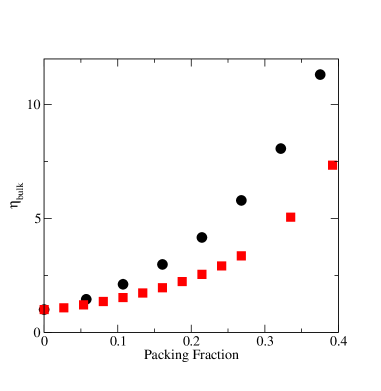
Figure 1: Shear viscosity computed in bulk conditions $\eta_{bulk}$ as a function of the packing fraction (this quantity should not be confused with the bulk viscosity of Section 4.1). Circles and squares are with and without the cross-over correction to viscosity, respectively.

Next, we address the classical question regarding how the confinement in a narrow space affects the viscosity of the fluid TravisGubbins ; Todd1 ; Todd2 . In our numerical tests, we consider the flow of a hard-sphere fluid between two parallel plates and observe the density and velocity profile. Since this a direct test of the viscosity of the fluid we expect a change with respect to the previous version where the terms $A_{ij}$ and $B_{i}$ were not taken into account. As shown in Fig.2 the measured viscosity converges for quite large channels of the order of $200$ lattice units towards the predicted bulk value, whereas for small values of the width $W$ is consistently lower, thus indicating that the walls strongly affect the motion of the adjacent layers.

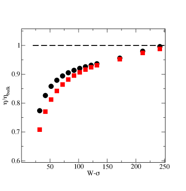
Figure 2: Normalized shear viscosity as a function of the effective slab width $(W-\sigma)$ expressed in lattice units. Circles and squares correspond to packing fractions of $0.11$ and $0.32$, respectively.

VI Conclusions

In this study we have considered the corrections to the transport coefficients which determine the cross terms between kinetic and collisional contributions. At the price of including a couple of extra contributions in the term describing the relaxation of fast modes, that is by lifting the BGK approximation for these modes, we have obtained a new estimate for the transport properties. After deriving an explicit expression for these quantities, we have evaluated the correction to viscosity via numerical simulations. It is interesting to remark that the range of validity of the presented LB algorithm does not extend to very low densities. The reason being that, if one assumes a constant relaxation frequency $\omega_{0}$, the value of the kinematic viscosity is too small and the small Knudsen number assumption breaks down.

The resulting form of the expression for the viscosity has similarities with the one derived within the local average density model (LADM) by Davis and coworkers Davis . They assumed that the functional dependence of transport coefficients on density can be computed via the corresponding expressions in the Enskog theory of hard-sphere fluids, by replacing the actual density $n({\bf r},t)$ by the coarse grained density, $\bar{n}({\bf r},t)$. An approximation very similar to the LADM can be derived within our method by using the explicit form of $\Omega$. Such a recipe is in the same spirit as the early weighted density density functional theories of equilibrium systems where the local free energy density was assumed to be a function of $\bar{n}({\bf r})$. Moreover, as pointed out by Hoang and Galliero in a Molecular Dynamics study Galliero , the LADM underestimates the importance of the local density as far as the kinetic term is concerned. The present theory, does not suffer from such a problem since it treats on a separate basis kinetic and potential terms.

Finally, the presence of attractive interactions can be accommodated in a mean field fashion by adding a Random Phase term in the evolution equation. However, while representing a very important contribution to the equation of state, such a modification does not modify the transport coefficients (with the notable exception of the interspecies diffusion coefficient in mixtures, see refs. KarkheckStell ; JCP2011B ). The reason for this shortcoming is that in the Enskog-like equation the details of the potential enter only through the cross-section.

Acknowledgments

U.M.B.M. acknowledges the support of the Project COFIN-MIUR 2009.

References

- (1) T.M. Squires and S.R. Quake, Rev.Mod.Phys. 77, 977 (2005).
- (2) R.B. Schoch, J.Han, P. Renaud, Rev.Mod.Phys. 80, 839 (2008).
- (3) H. Bruus, Theoretical Microfluidics, Oxford University Pres., New York, (2008).
- (4) B. J. Kirby, Micro and Nanoscale Fluid Mechanics, Cambridge University Press (2010).
- (5) L. Bocquet and E. Charlaix, Chem. Soc. Rev. 39, 1073, (2009).
- (6) S. K. Bhatia, M. R. Bonilla, and D. Nicholson, Phys. Chem. Chem. Phys. 13, 15350 (2011).
- (7) G. Karniadakis, A. Beskok, N. Aluru, Microflows and nanoflows, Springer, New York (2005).
- (8) L. Bocquet and J. L. Barrat, Phys. Rev. E 49, 3079 (1994).
- (9) R. Hartkamp, A. Ghosh, T. Weinhart, and S. Luding, J.Chem.Phys. 137, 044711 (2012)
- (10) L. A. Pohzar and K. E. Gubbins, J. Chem. Phys. 99, 8970 (1993).
- (11) J. G. Anero and P. Español, Europhys. Lett. 78, 50005 (2007).
- (12) A.J. Archer , J. Phys.: Condens. Matter 18, 5617 (2006).
- (13) U. Marini Bettolo Marconi and S.Melchionna, J. Chem. Phys. 126, 184109 (2007).
- (14) S. Succi, The lattice Boltzmann equation for fluid dynamics and beyond, 1th edition , Oxford University Press, (2001).
- (15) R. Benzi, S. Succi, M.Vergassola, Phys. Rep. 222, 145 (1992).
- (16) S. Melchionna and U. Marini Bettolo Marconi, Europhys. Lett. 81, 34001 (2008).
- (17) U. Marini Bettolo Marconi and S.Melchionna, J. Chem. Phys. 131, 014105 (2009).
- (18) U. Marini Bettolo Marconi, Mol. Phys. 109, 1265 (2011).
- (19) L.-S. Luo, Phys. Rev. Lett. 62, 1618, (1998).
- (20) P. Tarazona, Phys. Rev. A 31 2672 (1985).
- (21) See, e.g., R. Evans 1992 Fundamentals of Inhomogeneous Fluids ed. by D. Henderson (New York: Dekker)
- (22) W. Dufty, A. Santos, and J. Brey, Phys. Rev. Lett. 77, 1270 (1996).
- (23) H. van Beijeren and M.H. Ernst, Physica A, 68, 437 (1973), 70, 225 (1973).
- (24) P. L. Bhatnagar, E. P. Gross, and M. Krook, Phys. Rev. 94, 511 (1954).
- (25) U. Marini Bettolo Marconi and S. Melchionna, J. Phys.: Cond. Matt. 22, 364110 (2010).
- (26) U. Marini Bettolo Marconi and S. Melchionna, J. Chem. Phys. 134, 064118 (2011).
- (27) U. Marini Bettolo Marconi and S.Melchionna, J. Chem. Phys 135, 044104 (2011).
- (28) A. Santos, J.M. Montanero, J.W. Dufty and J.J. Brey, Phys. Rev. E 57, 1644 (1998).
- (29) H.J. Kreuzer, Non-equilibrium Thermodynamics and its Statistical Foundations Oxford University Press, New York (1981).
- (30) S.R. de Groot and P. Mazur, Non-equilibrium Thermodynamics Dover, New York (1984).
- (31) J.A. McLennan, Introduction to Non Equilibrium Statistical Mechanics, Prentice Hall, Indiana, (1988).
- (32) G. K. Batchelor An Introduction to Fluid Dynamics, Cambridge University Press, Cambridge (1967).
- (33) L.-S. Luo, Phys.Rev. E 81, 4982, (2000).
- (34) X. Shan and H. Chen, Phys. Rev. E 47, 1815 (1993).
- (35) M.R. Swift, W.R. Osborn, and J.M. Yeomans, Phys. Rev. Lett. 75, 830, 1995).
- (36) U. Marini Bettolo Marconi and P. Tarazona, J. Chem. Phys. 110, 8032 (1999) and J.Phys.: Condens. Matter 12, 413 (2000).
- (37) J. Fischer and M. Methfessel, Phys. Rev. A 22, 2836 (1980).
- (38) S. Melchionna and U. Marini Bettolo Marconi, Europhys.Lett 95, 44002 (2011).
- (39) S. Melchionna and U. Marini Bettolo Marconi, Phys. Rev. E, 85 036707 (2012).
- (40) H.C. Longuet-Higgins and J.A. Pople, J.Chem.Phys. 25, 884 (1956).
- (41) J-P. Hansen and I.R. McDonald, Theory of Simple Liquids, 3rd ed., Academic Press, London (2006).
- (42) S. Chapman and T.G. Cowling The mathematical Theory of Non-uniform Gases 3rd ed. Cambridge University Press, Cambridge (1970).
- (43) P. Travis and K. E. Gubbins, J. Chem. Phys. 112, 1984 (2000).
- (44) D. Todd, J. S. Hansen, and P. J. Daivis, Phys. Rev. Lett. 100, 195901 (2008).
- (45) D. Todd and J. S. Hansen, Phys. Rev. E 78, 051202 (2008).
- (46) I. Bitsanis, T.K. Vanderlick, M. Tirrell M., H.T. Davis, J. Chem. Phys. 89, 3152 (1988).
- (47) H. Hoang and G.Galliero J. Chem. Phys. 136, 124902 (2012).
- (48) J. Karkheck, E. Martina and G. Stell, Phys.Rev. A 25, 3328 (1982).