Primordial Non-Gaussianity and Reionization

Abstract

The statistical properties of the primordial perturbations contain clues about the origins of those fluctuations. Although the Planck collaboration has recently obtained tight constraints on primordial non-gaussianity from cosmic microwave background measurements, it is still worthwhile to mine upcoming data sets in effort to place independent or competitive limits. The ionized bubbles that formed at redshift $z\sim 6-20$ during the Epoch of Reionization are seeded by primordial overdensities, and so the statistics of the ionization field at high redshift are related to the statistics of the primordial field. Here we model the effect of primordial non-gaussianity on the reionization field. The epoch and duration of reionization are affected as are the sizes of the ionized bubbles, but these changes are degenerate with variations in the properties of the ionizing sources and the surrounding intergalactic medium. A more promising signature is the power spectrum of the spatial fluctuations in the ionization field, which may be probed by upcoming 21 cm surveys. This has the expected $1/k^{2}$ dependence on large scales, characteristic of a biased tracer of the matter field. We project how well upcoming 21 cm observations will be able to disentangle this signal from foreground contamination. Although foreground cleaning inevitably removes the large-scale modes most impacted by primordial non-gaussianity, we find that primordial non-gaussianity can be separated from foreground contamination for a narrow range of length scales. In principle, futuristic redshifted 21 cm surveys may allow constraints competitive with Planck.

I Introduction

The standard cosmological model makes predictions that have been confirmed in a variety of arenas, from the cosmic microwave background to large surveys of galaxies. The model contains three mysteries, elements that are not part of the Standard Model of particle physics: dark matter, dark energy, and inflation. Inflation currently plays the role of providing the seeds of structure, and the simplest inflationary models predict that the perturbations responsible for this structure were drawn from a gaussian distribution. Evidence for primordial non-gaussianity then would speak to either a more complex inflation model or an alternative in which early acceleration does not occur. Either would be fascinating and probe physics operating at the earliest moments in the history of our Universe.

The Planck Collaboration Ade:2013ydc has, however, recently – as we were completing this work – placed stringent constraints on primordial non-gaussianity, by determining a robust upper limit to the 3-point function of the cosmic microwave background Komatsu:2002db ; Creminelli:2005hu ; Smith:2009jr . These results provide support for the simplest models of inflation with gaussian primordial fluctuations; nature may not provide us with this potential handle on the physics of inflation and alternatives. Given the enormous significance of a detection of primordial non-gaussianity, it is nonetheless worth pursuing additional observational constraints. Since the cosmic microwave background is relatively unscathed by gravitational, non-linear effects, it will be challenging to improve on the Planck constraint or to confirm it independently. The two-point function of biased tracers (galaxies, clusters, etc.) Dalal:2007cu may, however, be able to provide competitive constraints.

While galaxy surveys have been the premier method of studying the large scale structure of the Universe, upcoming 21 cm surveys will map the distribution of neutral hydrogen and therefore provide another handle. Ultimately the large number of Fourier modes potentially accessible to 21 cm surveys, may allow even more stringent constraints than possible with galaxy surveys and the cosmic microwave background Loeb:2003ya . In principle, an extremely futuristic redshifted 21 cm survey could even detect the level of non-gaussianity expected from the simplest single field models of slow-roll inflation Cooray:2006km . The first aim of redshifted 21 cm surveys is, however, to map out the details of the reionization process at $z\sim 6-20$. Motivated in part by the ultimate promise of the redshifted 21 cm line as a probe of primordial non-gaussianity, we examine here whether measurements during the reionization epoch might themselves provide a useful probe. During reionization, initial halo formation triggered early star formation that produced radiation sufficient to ionize large bubbles. An important realization from the past decade of theoretical work is that regions with large scale over-densities are ionized before typical regions (e.g., Barkana:2003qk ; Furlanetto:2004nh ; Iliev:2005sz ; Zahn:2006sg ). This results because small scale halo formation is biased: halos preferentially form in large scale over-densities. Given that primordial non-gaussianity affects this biasing Dalal:2007cu , it is interesting to study the impact of non-gaussianity on reionization.

There have been several related studies in the past Crociani:2008dt ; Joudaki:2011sv ; Tashiro:2012wr ; Chongchitnan:2013oxa . Our work has most overlap with Ref. Joudaki:2011sv . These authors focused on the scale-dependent clustering of the ionized regions, while we additionally quantify the impact of primordial non-gaussianity on the timing of reionization and the size distribution of ionized regions, and compare with analytic predictions for the scale-dependent biasing signature. Furthermore, we consider the impact of foreground cleaning in more detail than previous authors. This may ultimately provide the largest obstacle for obtaining precise constraints on primordial non-gaussianity from redshifted 21 cm observations, and so we estimate its impact carefully here.

The outline of this paper is as follows. We study non-gaussianity and reionization here by combining the technologies developed by Furlanetto et al. Furlanetto:2004nh to model reionization and the path integral formalism of Ref. Maggiore:2009rx to quantify the impact of non-gaussianity. In §II, we review the Furlanetto model and explain how non-gaussianity impacts the collapse fraction and therefore the over-density threshold above which a large scale region will be considered ionized. Then, we carry out semi-numerical simulations in §III and show results for the bubble size and ionization history in non-gaussian models. Then, in §IV, we compute the two-point function of the ionization field in the simulations and demonstrate that the power spectrum rises on large scales. Finally, we conclude in §V by projecting how well upcoming 21 cm surveys will be able to measure this feature in the power spectrum in the presence of astrophysical foregrounds that pollute the large scale spectrum. We conclude in §VI.

II The FZH model and Non-Gaussianity

In effort to understand the impact of primordial non-gaussianity on the reionization process, we will extend the analytic reionization model of Ref. Furlanetto:2004nh (hereafter ‘FZH’) to the case of non-gaussian initial conditions. In order for this work to be self-contained we briefly summarize the FZH model here, but refer the reader to the original paper for a complete treatment. The crux of FZH is that galaxies form first in large scale overdense regions and that these regions hence reionize before typical parts of the Universe. Extended Press-Schechter (EPS) theory and the excursion set formalism Bond:1990iw describe how halo formation – and by extension galaxy formation – is enhanced in large scale overdense regions, and so we can apply EPS to model reionization. This technique most faithfully captures large scale variations in the timing of reionization; we anticipate that primordial non-gaussianity will have its most dramatic impact on precisely these large scale variations. Furthermore, upcoming redshifted 21 cm surveys will measure only the large scale features of reionization (e.g. Furlanetto:2006jb ; Lidz:2007az ). For these reasons, the FZH model is well-suited for our present purposes.

In order for a region to be reionized, the number of photons emitted by sources in the region must at least exceed the number of hydrogen atoms contained within the region. Since ionized atoms can recombine, it takes more than one photon per atom to reionize a patch of the Universe: recent simulations suggest that a few photons per atom should suffice (e.g. 2009MNRAS.394.1812P ). In the simplest variant of FZH that we follow here, one supposes that each galaxy, with total host halo mass $M_{\rm gal}$, can ionize a mass of hydrogen (accounting for some average number of recombinations) proportional to its host halo mass,

$$M_{\rm ion}=\zeta M_{\rm gal}.$$ (1)

Here $\zeta$ is an ionizing efficiency parameter that depends on the fraction of galactic baryons that are converted into stars, the number of ionizing photons that are produced per baryon converted into stars, the fraction of ionizing photons that escape galactic host halos and make it into the surrounding IGM, the average recombination rate in the IGM, and other factors. Plausible values for these quantities yield $\zeta\sim 10$, although with substantial uncertainties (e.g. Furlanetto:2006jb ).

We further assume that every dark matter halo above some minimum (total, i.e., dark matter plus baryons) mass, $M_{\rm min}$, hosts a galaxy. Throughout we assume that $M_{\rm min}$ is set by the mass scale at which the virial temperature is $10^{4}$ K, above which gas can dissipate thermal energy by emitting atomic lines, condense into the center of the halo, and eventually form stars. It provides a plausible lower limit for the host halo mass of a galaxy. At high redshifts where $\Omega_{m}(z)\approx 1$, the corresponding atomic cooling mass scale is Barkana:2000fd :

$$M_{\rm min}=1.2\times 10^{8}M_{\odot}\left(\frac{9}{1+z}\right)^{3/2}\left(\frac{T_{\rm vir}}{10^{4}K}\right)^{3/2}\left(\frac{0.27}{\Omega_{\rm m}}\right)^{1/2}.$$

(2)

Given these assumptions about the ionizing sources and recombinations in the IGM, FZH consider spheres of varying radius around every point in the IGM. Each gas parcel in the IGM is approximated to be either completely ionized or completely neutral. According to Equations 1 and 2, if a sufficiently large fraction of the matter contained in a given sphere is collapsed into galaxy-hosting halos, the region should be ionized by the sources within. In particular, suppose a region has overdensity $\delta_{m}$ when the linear density field is smoothed with a (real space) spherical top-hat of co-moving radius $R_{m}$, enclosing a Lagrangian mass $M_{m}=\langle\rho_{\rm m}\rangle 4\pi R_{m}^{3}/3$, with $\langle\rho_{\rm m}\rangle$ indicating the co-moving cosmic mean matter density. Let us further denote the variance of the linear density field on this smoothing scale by $S_{m}$, and the variance smoothed on mass scale $M_{\rm min}$ by $S_{n}$. The condition for the region to be ionized is then:

$$\zeta f_{\rm coll}(S_{n}|\delta_{m},S_{m})\geq 1.$$ (3)

Here the symbol $f_{\rm coll}$ refers to the collapse fraction in the region, i.e., to the fraction of matter in the region that is in halos of mass larger than $M_{\rm min}$. The minimum overdensity for which this condition is satisfied is given the label $\delta_{m}=\delta_{X}$. A given point in the IGM is considered to be part of an ionized region of size $R_{m}$ when $R_{m}$ is the largest smoothing scale for which this condition is satisfied. In the event that there is no smoothing scale around a given point for which this criterion is satisfied, the point is considered to be completely neutral.

With these assumptions, FZH treat reionization – in the language of excursion set theory – as a ‘barrier-crossing’ problem. In the excursion set formalism one considers the behavior of the smoothed field about a point, $\delta_{m}$, as a function of decreasing smoothing scale or equivalently increasing $S_{m}$; each realization of $\delta_{m}$ with increasing variance, $S_{m}$, is said to follow a ‘trajectory’. The statistical properties of the ionized regions then follow from considering the probability distribution that trajectories cross the barrier condition of Equation 3 at various smoothing scales.

In order to extend this treatment to the case of non-gaussian initial conditions, two steps are hence involved. First, we need to calculate the conditional collapse fraction in an overdense region, $f_{\rm coll}(S_{n}|\delta_{m},S_{m})$, for non-gaussian models. This in turn defines the reionization barrier – $\delta_{X}(S_{m})$ – through Equation 3. Second, we need to consider non-gaussian modifications to the probability distribution for trajectories to cross this barrier. A technical challenge with both of these steps is that non-gaussianity induces distinctive correlations between $\delta_{m}$ at different smoothing scales, which must be incorporated into these calculations. This complicates things considerably in comparison to the case considered by FZH. In the usual FZH model, barrier crossing probability distributions are calculated using a top-hat smoothing filter in $k$-space and assuming gaussian initial conditions. With these assumptions, different steps in a trajectory are uncorrelated: the future evolution of a trajectory with increasing variance is independent of its past history. This is the defining characteristic of a Markov process. Fortunately, Maggiore, Riotto and De Simone Maggiore:2009rv ; Maggiore:2009rw ; Maggiore:2009rx ; DeSimone:2010mu ; DeSimone:2011dn developed a path integral formulation of excursion set theory which allows one to study departures from the Markov case, including the mode-couplings induced by primordial non-gaussianity (see also the related works D'Amico:2010ta ; Paranjape:2011ak ; Musso:2012ch ; Musso:2012qk ).

II.1 Non-gaussian Models

Throughout the present work, we specify to the special case of local models of primordial non-gaussianity. In these models, the primordial curvature perturbation (on scales smaller than the horizon) is parametrized by:

$$\Phi({\mathchoice{{\hbox{\BFd x}}}{{\hbox{\BFt x}}}{{\hbox{\BFs x}}}{{\hbox{\BFss x}}}})=\phi_{G}({\mathchoice{{\hbox{\BFd x}}}{{\hbox{\BFt x}}}{{\hbox{\BFs x}}}{{\hbox{\BFss x}}}})+f_{\rm NL}\left[\phi_{G}^{2}({\mathchoice{{\hbox{\BFd x}}}{{\hbox{\BFt x}}}{{\hbox{\BFs x}}}{{\hbox{\BFss x}}}})-\langle\phi_{G}^{2}({\mathchoice{{\hbox{\BFd x}}}{{\hbox{\BFt x}}}{{\hbox{\BFs x}}}{{\hbox{\BFss x}}}})\rangle\right].$$ (4)

Here $\phi_{G}(x)$ is a gaussian random field and $f_{\rm NL}$ characterizes the strength of the non-gaussianity. This form produces a bispectrum that is peaked for squeezed triangles – i.e., for $k$-space triangles in which one wavevector has much smaller magnitude than the other two. Although the above form of primordial non-gaussianity is only one of many possibilities, it is the most well-studied, and is expected for a wide range of different scenarios, such as multi-field inflationary models. Recent Planck results provide tight constraints on these models, finding $f_{\rm NL}^{\rm local}=2.7\pm 5.8$ at $68\%$ confidence level Ade:2013ydc . We will nonetheless consider significantly larger values for $f_{\rm NL}$ in order to best illustrate the effects of primordial non-gaussianity on reionization. In addition to the local-type non-gaussianity considered here, it is also common to consider equilateral type non-gaussianity, which peaks for triangles with $k_{1}\approx k_{2}\approx k_{3}$, as well ‘folded’ and ‘orthognal’ triangle configurations (see e.g. Ade:2013ydc ). It may also be possible to improve on the Planck collabroation’s current $68\%$ confidence constraints on these other types of non-gaussianity, $f_{\rm NL}^{\rm equil}=42\pm 75$, and $f_{\rm NL}^{\rm ortho}=-25\pm 39$ Ade:2013ydc , but we don’t consider this explicitly here (although see Chongchitnan:2013oxa ).

II.2 The Reionization Barrier in Non-gaussian Models

We first consider how the reionization barrier is modified in models with primordial non-gaussianity. Adshead et al. Adshead:2012hs and D’Aloisio et al. DAloisiobias calculate the conditional collapse fraction in models with primordial non-gaussianity using a top-hat filter in k-space and the path integral formulation of the excursion set formalism from Maggiore:2009rx . For the special case of spherical collapse, Adshead et al.’s Equation (46) Adshead:2012hs gives an approximate form for the collapse fraction in a region of large-scale overdensity $\delta_{m}$. Retaining a few terms, dropped in the large scale limit that was taken in Adshead et al. Equation (46), we have:

$$f_{\rm coll}(S_{n}|\delta_{m},S_{m})\approx{\rm erfc}\left[\frac{\delta_{c}(z)-\delta_{m}}{\sqrt{2(S_{n}-S_{m})}}\right]$$

$$+\Bigg{\{}\frac{\langle\delta_{n}^{3}\rangle-\langle\delta_{m}^{3}\rangle+3\langle\delta_{m}^{2}\delta_{n}\rangle-3\langle\delta_{n}^{2}\delta_{m}\rangle}{3\sqrt{2\pi}(S_{n}-S_{m})^{3/2}}\left[\frac{(\delta_{c}(z)-\delta_{m})^{2}}{S_{n}-S_{m}}-1\right]$$

$$+\left(\langle\delta_{n}^{2}\delta_{m}\rangle+\langle\delta_{m}^{3}\rangle-2\langle\delta_{m}^{2}\delta_{n}\rangle\right)\frac{\delta_{m}}{S_{m}}\frac{\delta_{c}(z)-\delta_{m}}{\sqrt{2\pi(S_{n}-S_{m})^{3}}}\Bigg{\}}$$

$$\times{\rm exp}\left[-\frac{(\delta_{c}(z)-\delta_{m})^{2}}{2(S_{n}-S_{m})}\right].$$ (5)

Here $\delta_{c}(z)=1.686D(0)/D(z)$ is the critical overdensity for spherical collapse scaled to $z=0$ and $D(z)$ is the linear growth factor. The quantity $S_{n}$ is the variance of the linear density field, when the density field is smoothed on the scale $M_{\rm min}$, $S_{m}$ is the linear variance smoothed on large scale ($M_{m}$), and $\langle\delta_{n}^{3}\rangle$ is the skewness at smoothing scale $M_{\rm min}$. Similarly, $\langle\delta_{m}^{3}\rangle$ is the skewness smoothed on the large scale $M_{m}$, while $\langle\delta_{n}^{2}\delta_{m}\rangle$ and $\langle\delta_{m}^{2}\delta_{n}\rangle$ are cross terms that also arise in non-gaussian models. Each of these quantities is linearly evolved to the present day ($z=0$). The first term is the usual result for gaussian initial conditions from Press-Schechter theory, while the second and third terms are approximate modifications for a Universe with non-gaussian initial conditions. As detailed in Ref. Adshead:2012hs , the non-gaussian corrections – i.e., the second and third terms above – are derived assuming $\delta_{c}^{2}(z)\gg S_{m}$ and including only dominant three-point correlator terms. This expression is equivalent to D’Aloisio et al.’s Equation (32) DAloisiobias in the limit $\delta_{c}^{2}(z)\gg S_{m}$, $\delta_{c}(z)\gg\delta_{m}$, and ignoring their last term (i.e., the last line of their Equation (32), proportional to their ‘$\mathcal{C}$’), which is negligible for the case considered here.

For positive $f_{\rm NL}$, the conditional collapse fraction of Equation 5 is enhanced compared to the case of gaussian initial conditions. This results because positive $f_{\rm NL}$ enhances the high density tail of the probability distribution function and thereby boosts the chance of being above the collapse threshold, $\delta_{c}(z)$. In the large scale limit, where $S_{n}\gg S_{m}$, the correlators $\langle\delta_{m}^{3}\rangle$ and $\langle\delta_{m}^{2}\delta_{n}\rangle$ are small compared to $\langle\delta_{n}^{3}\rangle$ and $\langle\delta_{n}^{2}\delta_{m}\rangle$, and so the corresponding terms in Equation 5 are only significant close to the minimum mass scale, $M_{\rm min}$ ($S_{n}$). Furthermore, note that in the very large scale limit, $\langle\delta_{n}^{2}\delta_{m}\rangle/S_{m}\propto\sqrt{1/S_{m}}\rightarrow\infty$, i.e., this term diverges towards large scales. This divergence is not a concern since the density contrast, $\delta_{m}$, is itself tending towards zero on large scales. The $\langle\delta_{n}^{2}\delta_{m}\rangle$ correlator in the expression here describes the mode-coupling between large and small scales and it is this term that ultimately leads to the scale-dependent halo clustering signature (e.g., Adshead:2012hs ). Presently, we are interested in the impact of this term on the reionization barrier. Since it causes the conditional collapse fraction to blow-up on large smoothing scales (for positive $f_{\rm NL}$), it leads to a down-turn in the reionization barrier at small $S_{m}$. In the case of negative $f_{\rm NL}$, the sign of this effect is reversed and the reionization barrier turns-up at small $S_{m}$. We caution that approximations made in Equation 5 may influence the shape of the barrier on the largest scales here, and so we caution against taking this too literally. The behavior of the barrier on these scales does not, however, impact our results.

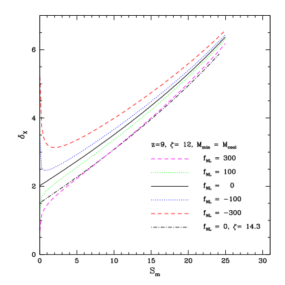
Figure 1: FZH reionization barrier for various $f_{\rm NL}$ models. The lines show the critical overdensity for a region to be ionized as a function of the linear variance when the density field is smoothed on the scale of the region (with both quantities linearly extrapolated to $z=0$). Each curve is for $z=9$, and assumes that galaxies form in halos above the atomic cooling mass, $M_{\rm cool}$, with an ionizing efficiency parameter of $\zeta=12$. For $f_{\rm NL}=0$, the volume-averaged ionization fraction is $\langle x_{i}\rangle=0.48$ at this redshift. The collapse fraction in a region of large-scale overdensity increases with increasing $f_{\rm NL}$ and so the critical overdensity for a region to be ionized, $\delta_{X}$ decreases with increasing $f_{\rm NL}$. The black dot-dashed line is a $f_{\rm NL}=0$ model with $\zeta$ adjusted to match the volume-averaged ionization fraction in the $f_{\rm NL}=300$ model (see text).

In order to quantify the impact of $f_{\rm NL}$ on the shape of the reionization barrier, we invert Equations 3 and 5 to find $\delta_{X}$ as a function of $S_{m}$ for several $f_{\rm NL}$ models. Here we generally consider $z=9$, $\zeta=12$, and set $M_{\rm min}$ to the atomic cooling mass corresponding to a virial temperature of $T_{\rm vir}=10^{4}K$, as specified by Equation 2. For $f_{\rm NL}=0$ these parameters give $\langle x_{i}\rangle=0.48$, and so we are considering roughly the ‘mid-point’ of reionization, where half of the volume of the Universe is ionized. The results of these calculations are shown in Figure 1 for models with $f_{\rm NL}=(-300,-100,0,100,300)$. The barrier decreases with increasing $f_{\rm NL}$: positive $f_{\rm NL}$ boosts the conditional collapse fraction in overdense regions, and hence a lower critical overdensity $\delta_{X}$ is required for a region to be ionized in a non-gaussian model. The barrier turns down (up) significantly on large scales for positive (negative) $f_{\rm NL}$ because the collapse fraction blows up towards large scales, as mentioned earlier. Even for values as large as $|f_{\rm NL}|\sim 100$ – now strongly disfavored by the Planck constraints Ade:2013ydc – this down-turn (up-turn) occurs on rather large scales, where the barrier-crossing probability should be very small. In general, $f_{\rm NL}$ leads to only small changes in the barrier height and shape. For instance, $\delta_{X}$ is $\sim 8\%$ smaller at $R=3$ Mpc/$h$ ($S_{m}\approx 3$) and $\sim 15\%$ smaller at $R=10$ Mpc/$h$ ($S_{m}\approx 0.5$) in the $f_{\rm NL}=100$ model compared to the gaussian, $f_{\rm NL}=0$, case. The scale $R=3$ Mpc/$h$ mentioned here corresponds to the peak in the analytic bubble size distribution for the $f_{\rm NL}=0$ model, computed as in Furlanetto:2004nh , while $\sim 99\%$ of bubbles in this model have $R\leq 10$ Mpc/$h$, the second scale considered here. These numbers hence give some indication of which scales typically cross the reionization barrier in these models.

In addition, the impact of $f_{\rm NL}$ on the reionization barrier at a given redshift is largely degenerate with the effect of varying $\zeta$. This is illustrated by the black dot-dashed line in Figure 1, which shows an $f_{\rm NL}=0$ model with $\zeta$ enhanced (from $\zeta=12$ to $\zeta=14.3$) to match the volume-averaged ionization fraction in the $f_{\rm NL}=300$ model at this redshift. The shapes of the barriers are somewhat different; the barrier in the $f_{\rm NL}$ model has the large scale down-turn and rises more steeply on small smoothing scales. The non-gaussian model should have slightly more large bubbles and slightly fewer small bubbles than a gaussian model with the same volume-averaged ionization fraction (see §III for further details). However, from a similar bubble-size distribution calculation to the one mentioned above, we expect $\sim 99\%$ of random walks in the $f_{\rm NL}=0$, $\zeta=14.3$ model (that is largely degenerate with the $f_{\rm NL}=300$ model) to cross the barrier at $S_{m}\gtrsim 0.4$. This suggests that the most prominent differences between the two barriers, on large smoothing scales, will have little impact on the resulting bubble-size distributions since few random walks cross the barrier on such large scales, at least near the middle of reionization. Hence it seems that varying $\zeta$ should largely compensate for $f_{\rm NL}$ induced changes in the reionization barrier. In addition, we should keep in mind that the values of $f_{\rm NL}$ considered here are already strongly disfavored by existing data, and so the degeneracy is even more important than in this illustrative case.

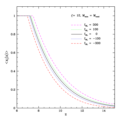
Figure 2: Volume-averaged ionization fraction vs. redshift for various $f_{\rm NL}$ models. The curves show the impact of $f_{\rm NL}$ on the reionization history of the Universe in models with $M_{\rm min}=M_{\rm cool}$ and $\zeta=12$. The reionization process is accelerated in a Universe with positive $f_{\rm NL}$, while it is delayed in a Universe with negative $f_{\rm NL}$.

A similar calculation determines the volume-averaged ionization fraction as a function of redshift in the FZH model. Specifically, this is given by:

$$\langle x_{i}\rangle=\zeta f_{\rm coll}(S_{n})$$

$$=\zeta{\rm erfc}\left[\frac{\delta_{c}(z)}{\sqrt{2S_{n}}}\right]+\zeta\frac{\langle\delta_{n}^{3}\rangle}{3\sqrt{2\pi}S_{n}^{3/2}}\left[\frac{\delta_{c}^{2}(z)}{S_{n}}-1\right]{\rm exp}\left[-\frac{\delta_{c}^{2}(z)}{2S_{n}}\right].$$ (6)

This equation holds for redshifts above which the ionized fraction, $\langle x_{i}\rangle$, becomes unity. Here $f_{\rm coll}(S_{n})$ is the (non-conditional) collapse fraction for halos above the minimum mass at any given redshift. This is specified by Equation 5 in the limit that $M_{m}\rightarrow\infty$, $\delta_{m}\rightarrow 0$. Since the collapse fraction is enhanced in models with positive $f_{\rm NL}$, so is the volume-averaged ionization fraction. This is quantified in Figure 2, which shows the volume-averaged ionization fraction as a function of redshift in the $f_{\rm NL}$ models of Figure 1. As before, we fix $\zeta=12$ in each model and the minimum host halo mass at the atomic cooling mass. Reionization starts and finishes earlier (later) in models with positive (negative) $f_{\rm NL}$ compared to models with gaussian initial conditions. However the effects are small: for instance, the ionization fraction near $\langle x_{i}\rangle=0.5$ is boosted by $\lesssim 10\%$ for $f_{\rm NL}=100$.

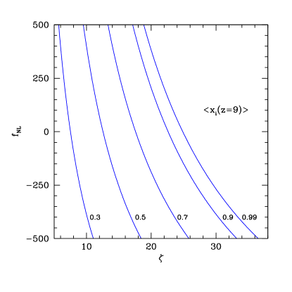
Figure 3: Contours of constant ionized fraction in the $\zeta-f_{\rm NL}$ plane. The blue lines are lines of constant ionized fraction, with $\langle x_{i}(z=9)\rangle=0.3,0.5,0.7,0.9$ and $0.99$ respectively, illustrating the degeneracy between $f_{\rm NL}$ and $\zeta$.

The impact of $f_{\rm NL}$ on the volume-averaged ionization fraction is, however, degenerate with uncertainties in the ionizing efficiency and the minimum host halo mass, which are unknown and in any case provide only a rough model for $\langle x_{i}\rangle(z)$. We illustrate this degeneracy in Figure 3, which shows contours of constant $\langle x_{i}(z=9)\rangle$. The plot spans a very large range in $f_{\rm NL}$, including models that are already strongly disfavored by existing data for illustration. The steepness of the contours indicates that relatively small variations in $\zeta$ can compensate for $f_{\rm NL}$-induced changes, even over the large range in $f_{\rm NL}$ shown. In Figure 1 we found that the reionization barrier in an $f_{\rm NL}$ model nearly matches that in a gaussian model, once we adjust $\zeta$ to fix $\langle x_{i}\rangle$ across models. This suggests that the bubble size distribution will mostly share this degeneracy: in other words, the contours of fixed $\langle x_{i}\rangle$ in Figure 3 should resemble contours of fixed bubble-size distribution as well. We will explore more distinctive and unique imprints of primordial non-gaussianity subsequently.

III Semi-Numeric Simulations and Non-gaussianity

In order to calculate the statistics of the ionized regions, such as their size distribution, we need to consider the probability that trajectories cross the barrier of Equation 3 at various smoothing scales. Here we will handle this numerically, using the so-called ‘semi-numeric’ simulation technique developed in Zahn:2006sg . This simulation technique is essentially a (three dimensional) Monte-Carlo implementation of the FZH model. The Monte-Carlo implementation has the advantage that it partly captures asphericity in the shapes of the ionized regions, (which we will sometimes refer to as ‘ionized bubbles’). Furthermore, it provides mock reionization data cubes that are convenient for measuring the statistical properties of the epoch of reionization, and for visualizations. In comparison to radiative transfer simulations of reionization, the semi-numeric Zahn:2006sg technique has the advantage that it is extremely fast, while still capturing the large scale features of the reionization process fairly accurately Zahn:2006sg ; Zahn:2010yw .

In order to use this technique to study reionization in an $f_{\rm NL}$ model, we need to first generate a non-gaussian realization of the linear density field in the model of interest. We do this in the usual manner, briefly described here for completeness. Specifically, we start by generating a gaussian random realization of the gaussian field $\phi_{G}({\mathchoice{{\hbox{\BFd x}}}{{\hbox{\BFt x}}}{{\hbox{\BFs x}}}{{\hbox{\BFss x}}}})$. In generating this realization, we assume that $\phi_{G}({\mathchoice{{\hbox{\BFd x}}}{{\hbox{\BFt x}}}{{\hbox{\BFs x}}}{{\hbox{\BFss x}}}})$ has a scale invariant power spectrum of the form $\Delta^{2}_{\phi}(k)=k^{3}P_{\phi}(k)/(2\pi^{2})=8.71\times 10^{-10}$. From $\phi_{G}({\mathchoice{{\hbox{\BFd x}}}{{\hbox{\BFt x}}}{{\hbox{\BFs x}}}{{\hbox{\BFss x}}}})$, we generate the primordial curvature perturbation assuming the local model described by Equation 4. The density field then follows from the potential perturbation by Poisson’s Equation, which may be written (and applied) in Fourier space as:

$$\delta({\mathchoice{{\hbox{\BFd k}}}{{\hbox{\BFt k}}}{{\hbox{\BFs k}}}{{\hbox{\BFss k}}}},z)=\frac{2c^{2}k^{2}T(k)D(z)\Phi({\mathchoice{{\hbox{\BFd k}}}{{\hbox{\BFt k}}}{{\hbox{\BFs k}}}{{\hbox{\BFss k}}}})}{3H_{0}^{2}\Omega_{\rm m}}.$$ (7)

Finally, we Fourier-transform the resulting density field into real space. In each model considered, the same set of random numbers are used to generate the underlying gaussian random potential field, $\phi_{G}({\mathchoice{{\hbox{\BFd x}}}{{\hbox{\BFt x}}}{{\hbox{\BFs x}}}{{\hbox{\BFss x}}}})$. This lessens the impact of sample variance when comparing different models, and isolates the impact of primordial non-gaussianity.

We generate models with $f_{\rm NL}=-100,-50,0,50,100,300$ in two different simulation volumes. The first simulation volume has a co-moving side length of $L_{\rm box}=150$ Mpc/$h$, while the second simulation has $L_{\rm box}=2$ Gpc/$h$. In each case, the density and ionization fields are tabulated on a $512^{3}$ Cartesian grid. The smaller simulation box captures small reionization bubbles, while the larger volume runs are essential for examining the large scale clustering of the ionized regions, especially the distinctive scale-dependent signatures induced by primordial non-gaussianity.

In order to construct the ionization field from a realization of the linear density field, we use the procedure of FZH and Zahn:2006sg . We smooth the linear density field on a range of scales, starting from large scales and gradually stepping down to the size of the simulation pixels. A pixel is marked as ionized if it crosses the barrier of Equations 3 and 5 on some smoothing scale, while pixels that fail to cross the barrier on any smoothing scale are marked neutral. Since we have proper non-gaussian realizations of the density field, the enhanced probability of crossing the reionization barrier in $f_{\rm NL}$ models is naturally accounted for in this step.

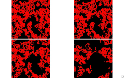
Figure 4: Slices through semi-numeric simulations of reionization models with primordial non-gaussianity. In each model, $\zeta=12,z=8$. The slices are $150$ co-moving Mpc/$h$ on a side, and are $0.29$ Mpc/$h$ thick. Top Left: $f_{\rm NL}=-100$, Top Right: $f_{\rm NL}=0$, Bottom Left: $f_{\rm NL}=100$, Bottom Right: $f_{\rm NL}=300$. The black regions show ionized bubbles, while the red regions are neutral gas. As $f_{\rm NL}$ increases, reionization is more progressed (for fixed ionizing efficiency, $\zeta$, and redshift, $z$), and the bubbles are larger.

We show example slices through $150$ Mpc/$h$ semi-numeric reionization simulations with $\zeta=12$ and $z=8$ in Figure 4. Since each simulation is generated with the same underlying gaussian random part of the potential field, $\phi_{G}({\mathchoice{{\hbox{\BFd x}}}{{\hbox{\BFt x}}}{{\hbox{\BFs x}}}{{\hbox{\BFss x}}}})$, we can compare the slices directly, region-by-region. As expected, reionization has progressed further, and the ionized regions are larger, in the models with primordial non-gaussianity. In the $f_{\rm NL}=\pm 100$ model, however, the differences with the case of gaussian initial conditions are somewhat subtle. Note that we are comparing the different models at fixed $\zeta$ and $z$, and so the models have varying volume-averaged ionization fractions, which increase with $f_{\rm NL}$. Specifically, the model with $f_{\rm NL}=0$ has $\langle x_{i}\rangle=0.45$ at $z=8$, while $\langle x_{i}\rangle=(0.40,0.50,0.63)$ for $f_{\rm NL}=(-100,100,300)$ at $z=8$. A caveat here is that these values are smaller than expected from the analytic curves in Figure 2, and the difference with the expected value decreases with increasing $|f_{\rm NL}|$. The smaller values result for two reasons: first, there are some ionized bubbles that are smaller than the size of our simulation grid and hence not captured. This effect is more important at small $|f_{\rm NL}|$ since the bubbles are smaller in these models. Second, our collapse-fraction expressions are derived using a top-hat filter in $k$-space but applied with a real-space filter: as discussed in the Appendix of Zahn:2006sg , this leads to departures from the expected global ionized fraction. Since the departure decreases with increasing $f_{\rm NL}$, our semi-numeric simulations likely overestimate the impact of $f_{\rm NL}$ on the ionized fractions and bubble-sizes, but they still serve to illustrate the main effects of non-gaussianity on reionization.

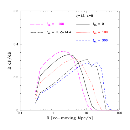
Figure 5: Bubble-size distribution for various $f_{\rm NL}$ models. The curves show the probability distribution of the sizes of the ionized regions for $x_{\rm th}=0.9$ (see text). The models are at $z=8$ and most assume $\zeta=12$, $M_{\rm min}=M_{\rm cool}$, for various values of $f_{\rm NL}$ as labeled. The black dot-dashed model is for an $f_{\rm NL}=0$ model with $\zeta$ adjusted to match the mean ionized fraction ($\langle x_{i}\rangle$) in the $f_{\rm NL}=300$ model. This illustrates that the variations in bubble size with $f_{\rm NL}$ at fixed $\langle x_{i}\rangle$ are much smaller than at fixed $\zeta$.

In order to quantify the visual impressions of Figure 4, we calculate the probability distribution of the sizes of the ionized regions for each $f_{\rm NL}$ model. This depends somewhat on one’s definition for the size of the complex, aspherical ionized regions in the simulation. Here we define the size of the simulated ionized regions as in Zahn:2006sg . Briefly, we spherically average the ionization field on various scales $R$, starting from large scales, stepping downward in size until we eventually get to the size of our simulation pixels. At each smoothing scale, we compare the spherically averaged ionization field to a threshold ionization value, $x_{\rm th}$. A simulation pixel is considered ‘ionized’ and belonging to a bubble of radius $R$, when $R$ is the largest smoothing radius at which the smoothed ionization field crosses the threshold. Pixels that do not cross the threshold on any smoothing scale are considered neutral. This procedure is of course similar to the way in which the ionization field is constructed in the first place.

The resulting probability distribution function (PDF), for $x_{\rm th}=0.9$, is shown for our various $f_{\rm NL}$ models with $\zeta=12$, $z=8$ in Figure 5. Note that each PDF is normalized to $1$ rather than to the ionized fraction: the PDFs show the fraction of bubbles that have a radius between $R$ and $R+dR$. To mention one quantitative description of these results, we examine by how much the characteristic size of ionized bubbles – which we identify with the peak in the bubble size PDFs of Figure 5 – varies with $f_{\rm NL}$ for the present values of $\zeta,z$. Compared to a model with gaussian initial conditions, the characteristic bubble size increases by a factor of $1.4$ for $f_{\rm NL}=100$, a factor of $3.7$ for $f_{\rm NL}=300$, while it decreases by a factor of $1.5$ for $f_{\rm NL}=-100$. As anticipated in the previous section, the bubble-sized distribution is degenerate with $\zeta$. The black dot-dashed line shows that an $f_{\rm NL}=0$ model with $\zeta$ adjusted upward to match the ionized fraction in the $f_{\rm NL}=300$ model. The resulting bubble-size distributions are quite similar, although the bubbles are a little bit larger in the $f_{\rm NL}$ model. This is expected from Figure 1; the main difference between the $f_{\rm NL}$ barrier and the gaussian barrier at fixed $\langle x_{i}\rangle$ is that the $f_{\rm NL}$ barrier is a little lower on larger scales (smaller $S_{m}$) allowing slightly larger ionized regions to form.

One might wonder whether random walks can start to cross the reionization barrier at very low $S_{m}$ in non-gaussian models, where the barrier has this distinctive downturn. In principle, this might lead to a bi-modality in the bubble size distribution: perhaps the downturn allows some trajectories to cross the barrier on very large scales that would be prohibited from crossing otherwise. On smaller smoothing scales, the trajectory-crossing probability might shrink as the smoothing scale becomes smaller than the down-turn scale and the barrier increases, until trajectories catch up again close to the scale of the usual peak in the bubble size distribution. This might imprint a distinctive large-scale bump in the bubble size distribution. It is possible that this is even the origin of the kink in the high-$R$ tail of the $f_{\rm NL}=300$ model in Figure 5. This effect might be more realizable at the end of reionization, when random walks start crossing the reionization barrier on progressively larger scales. However, this effect is unlikely important for the much smaller values of $f_{\rm NL}$ presently allowed, and so we don’t investigate it further here. It also may be an artifact of approximations made in deriving Equation 5, as mentioned earlier.

IV Scale-dependent Bias

The previous results describe the general impact of primordial non-gaussianity on reionization. However, the most promising approach for obtaining observational constraints on non-gaussianity from reionization studies is to measure the scale dependent clustering of the ionized regions. This is directly analogous to the case of the clustering of dark matter halos. In the case of halo clustering, Dalal et al. Dalal:2007cu showed that local non-gaussian models give rise to a scale-dependent clustering signature. If a similar signature arises in the clustering of ionized regions, this may provide a distinctive indicator and allow constraints on $f_{\rm NL}$ from the epoch of reionization, despite uncertainties in the properties of the ionizing sources, and the surrounding IGM.

Indeed, we would expect the ionized regions to have a similar scale-dependent clustering signature to that of the dark matter halos. In terms of excursion set modeling, the reionization case is different than halo clustering only in that the reionization barrier (Equation 3) has a different shape than the halo collapse barrier. Otherwise the physics underlying the scale dependent clustering is similar. In particular, a positive value of $f_{\rm NL}$ implies that the variance of the density field is enhanced in large scale regions with above average potential perturbation (which are overdense on large scales as quantified by the Poisson Equation, Equation 7.) The enhanced variance boosts the collapse fraction in such regions, and increases the tendency for these regions to be ionized before typical regions. In the context of the FZH model, the extra variance in large scale overdense regions boosts the rate at which trajectories cross the barrier of Equation 3 just as it increases the rate of crossing the spherical collapse barrier in the case of halo clustering. In both cases the form of Equation 7 then implies a distinctive scale-dependent clustering term, $\propto 1/(k^{2}T(k))$ Dalal:2007cu . Moreover, we Adshead:2012hs (see also DAloisiobias ) showed that this general form is expected for an arbitrary barrier crossing problem in the presence of primordial non-gaussianity with a non-zero squeezed limit. One caveat in the reionization case is that we expect this to apply only on scales much larger than the size of the ionized regions. On smaller scales, the ionization field will decorrelate from the underlying density field since small scale regions are either highly ionized or completely neutral irrespective of the precise value of the density field.

Our aim here is to quantify the scale-dependent clustering of the ionized regions. In order to capture the large scale Fourier modes where the scale-dependent clustering signature should dominate, we use $2$ Gpc/$h$ semi-numeric reionization simulations. As before, we construct simulations for several values of $f_{\rm NL}$; here we simulate $f_{\rm NL}=0,\pm 50,\pm 100$. We further calculate the power spectrum of the ionization field in each model, $P_{x,x}(k)$. We also calculate the ionization-density cross power spectrum, $P_{x,\delta_{\rho}}(k)$ and the density power spectrum, $P_{\delta_{\rho},\delta_{\rho}}(k)$. We then estimate the bias of the ionization field from the ratio of the ionization-density cross power spectrum and the density power spectrum,

$$b_{x}(k)=P_{x,\delta_{\rho}}(k)/P_{\delta_{\rho},\delta_{\rho}}(k).$$ (8)

As discussed previously, we expect primordial non-gaussianity to slightly lower the collapse barrier of Equation 3 (for positive $f_{\rm NL}$, as illustrated in Figure 1), and for the enhanced high density tail in these models to increase the probability of crossing the reionization barrier. The latter effect, and the coupling between large and small scale modes, is responsible for the scale dependent clustering enhancements. However, each of these two effects modifies the bias of the ionized regions, $b_{x}(k)$. Since $f_{\rm NL}$ is known to be small, we can consider each effect as a small correction in a Taylor expansion around $f_{\rm NL}=0$, and calculate the two effects separately. The change in bias from the reduced barrier height in a positive $f_{\rm NL}$ model is mainly due to the fact that the ionization fraction is larger (than gaussian). For small changes in $f_{\rm NL}$, and on scales much larger than the ionized regions, this leads to a roughly scale-independent change in $b_{x}(k)$. We find that this scale-independent term is fairly well matched by considering the change in bias in an $f_{\rm NL}=0$ model after adjusting $\zeta$ to match the enhanced $\langle x_{i}\rangle$ in the corresponding $f_{\rm NL}$ model (see Figure 6 for an illustration).

The second effect – increased probability of barrier crossing in a non-gaussian model – produces a distinctive scale-dependent clustering enhancement of the Dalal:2007cu form:

$$\Delta b_{x}(k)=\frac{3H^{2}_{0}\Omega_{\rm m}f_{\rm NL}(b_{x}^{G}-1)}{c^{2}k^{2}T(k)D(z)}\delta_{B}.$$ (9)

Here $\Delta b_{x}(k)$ denotes the change in bias with wavenumber $k$ owing to $f_{\rm NL}$, and the above equation describes only the scale dependent contribution. The quantity $b_{x}^{G}$ is the bias of the ionization field in a gaussian model, and $T(k)$ is the transfer function. Here $\delta_{B}$ is a proportionality constant related to the height of the reionization barrier. Note that $b_{x}^{G}$ and $\delta_{B}$ depend on both redshift/ionization fraction and the reionization model. The growth factor here, $D(z)$, is the linear growth factor normalized to $1/(1+z)$ during the matter-dominated era.

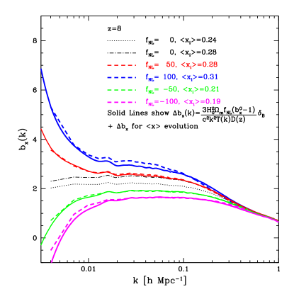
Figure 6: Scale-dependent bias of ionization field. The dashed lines show measurements of $b_{x}(k)$ (Equation 8) from semi-numeric simulations for $z=8$ and fixed $\zeta=12$. The solid lines show (by eye) fits to the simulation results. The fits consist of two terms. The first term is a scale dependent enhancement in the form of Equation 9, with the proportionality constant, $\delta_{B}$, adjusted to (roughly) match the $f_{\rm NL}=50$ measurement. The second term is predicted by varying $\zeta$ in a gaussian model to match the $\langle x_{i}\rangle$ value in the corresponding $f_{\rm NL}$ model. As an illustrative example, the dot-dashed line shows $b_{x}(k)$ for an $f_{\rm NL}=0$ model with the same $\langle x_{i}\rangle$ as for $f_{\rm NL}=50$. The difference between the dashed and dot-dashed lines hence reflects the roughly scale-independent (on large scales) correction to the bias for $f_{\rm NL}=50$, while the enhancement at $k\lesssim 0.02h$ Mpc^-1 is dominated by the scale-dependent contribution.

Our numerical results mostly perform this perturbative analysis, as shown in Figure 6 for $z=8$ and $\zeta=12$. We adjust the single parameter $\delta_{B}$ in Equation 9 above to match the simulation results, and calculate the scale-independent correction to the bias as described above. The result is shown by the solid curves in Figure 6. The fit is a fairly good overall match to the simulation results, although some differences are evident. Most importantly, one can see the scale-dependent enhancement of the Dalal et al. Dalal:2007cu type on large scales, and that this term is linear in $f_{\rm NL}$, as expected. (Note that the ‘fit’ curves share noisy features with the simulation results, because the scale independent correction is calculated directly from the simulated power spectra.)

The fits, however, seem to slightly underproduce the large scale enhancement for $f_{\rm NL}=100$, and slightly overproduce the effect at $f_{\rm NL}=-100$. The departure from the fits at large $f_{\rm NL}$ likely results because the change in the scale-independent bias in these models is becoming significant and is not perfectly captured by matching to a fixed $\langle x_{i}\rangle$. After all, the reionization barrier and bubble size distribution still differ slightly after matching to a fixed $\langle x_{i}\rangle$ (see Figure 1). Along these lines, we find a better fit if, in calculating the scale-independent correction, we boost $\zeta$ a bit beyond that required to match the enhanced $\langle x_{i}\rangle$ in the non-Gaussian model (although this improvement is not shown in the figure here). Quantitatively, we find $(b_{x}^{G}-1)\delta_{B}\approx 0.49$ for the redshift and ionization fraction considered here. This coefficient also depends on the particular reionization model considered here, e.g., the assumption that the ionizing efficiency in Equation 1 is itself independent of mass. Note that we considered the scale-dependent bias of $x_{i}$ here, if we had instead considered the field $\delta_{x}=(x_{i}-\langle x_{i}\rangle)/\langle x_{i}\rangle$ the scale dependent bias coefficient would be $\approx 2$.

The relatively good match emboldens us to use the simple fitting formula of Equation 9 in §V to project how well future 21 cm surveys will be able to extract $f_{\rm NL}$. The imperfect fit does, however, suggest that more theoretical work will be needed to extract the exact value of $f_{\rm NL}$ from the data.

Note that the scale dependent enhancement dominates over the variation from the enhanced $\langle x\rangle$ only on very large scales (small $k$), $k\lesssim 0.02h$ Mpc^-1. Unfortunately, these scales will likely be challenging to observe (see §V). In practice, the efficiency of the ionizing sources and their host halo masses will not be known a priori and so we will likely need to perform a joint fit for the scale independent and scale dependent bias contributions. If $\langle x_{i}\rangle(z)$ can be determined from independent observations, this would be helpful in separating out the scale dependent enhancement.

We also investigated how the results depend on the particular stage of the reionization process, by considering an additional model in which $\zeta$ is enhanced beyond our fiducial values of $\zeta=12$. In the alternate case considered, $\langle x_{i}\rangle=0.51$ at $z=8$ (for $f_{\rm NL}=0$) and so it describes the impact of non-gaussianity near reionization’s midpoint. In this case, we find a similar fit works, especially if we allow a slight boost to the scale-independent term, beyond that required to match to a fixed $\langle x_{i}\rangle$. At this stage of reionization, we find $(b_{x}^{G}-1)\delta_{B}\approx 0.35$. The proportionality constant in the fit of Equation 9 hence varies with $\zeta$, but this is to be expected since the proportionality constant should depend on the barrier height, which itself depends on $\zeta$. In principle, one can also consider later stages in reionization, but we expect this to be less useful. First, the signal drops off towards the end of reionization (e.g. Lidz:2007az ). Second, note that the ionization and density fields decorrelate on scales less than the size of the ionized regions. As the ionized bubbles grow, only larger and larger scales are useful for the scale-dependent clustering signature.

It is also possible to compute the scale-dependent bias coefficient, $(b_{x}^{G}-1)\delta_{B}$, analytically. The analytic calculations allow one to quickly explore many $f_{\rm NL}$ models for a wide range of ionized-fractions, $\langle x_{i}\rangle$, and redshifts. Ref. Adshead:2012hs has derived expressions for the scale-independent bias and scale-dependent bias coefficient that are applicable to any collapse barrier using a path integral approach developed by Maggiore:2010I ; Maggiore:2010II ; Maggiore:2010III . Following Adshead:2012hs , we define $\mathcal{P}_{0}(S_{m})$ as an expansion in the barrier:

$$\mathcal{P}_{0}(S_{m})=\sum_{p=1}^{5}\frac{-S_{m}^{p}}{p!}\frac{d^{p}}{dS_{m}^{p}}\delta_{X}(S_{m}).$$ (10)

The scale-independent part of the bias can then be written as

$$b_{x}^{G}(S_{m})=1+\frac{\delta_{X}(S_{m})D(0)}{D(z)S_{m}}-\frac{D(0)}{D(z)(\delta_{X}(S_{m})+P_{0}(S_{m}))}$$

which reduces to the standard expression from e.g. McQuinn:2005 in the limit that the barrier is linear. Since $\delta_{X}(S_{m})$ and $S_{m}$ are linearly extrapolated to $z=0$, the growth factor enters here in calculating the bias at redshift $z$. For an $f_{\rm NL}$ cosmology the scale-dependent bias can be written Adshead:2012hs

$$b^{\rm SD}(k)=\frac{2f_{\rm NL}}{\mathcal{M}(k)}c(S_{m})$$ (12)

where the coefficient $c(S_{m})$ is defined

$$c(S_{m}) = \delta_{X}(S_{m})(b_{x}^{G}-1)\frac{D(z)}{D(0)}-\frac{3\mathcal{P}_{0}(S_{m})}{\delta_{X}(S_{m})+\mathcal{P}_{0}(S_{m})}$$ (13)

$$+\left(2\sqrt{\frac{2\pi}{S_{m}}}\frac{\mathcal{P}^{2}_{0}(S_{m})}{(\delta_{X}(S_{m})+\mathcal{P}_{0}(S_{m}))}\right)$$

$$\times\text{exp}\left[\frac{\delta_{X}^{2}(S_{m})}{2S_{m}}\right]\text{erfc}\left[\frac{\delta_{X}(S_{m})}{\sqrt{2S_{m}}}\right].$$

and

$$\mathcal{M}(k)=\frac{2}{3}\frac{c^{2}k^{2}T(k)D(z)}{\Omega_{m}H_{0}^{2}}$$ (14)

In the limit that barrier is flat, i.e. $\delta_{X}(S_{m})=\delta_{c}$, then $\mathcal{P}_{0}(S_{m})=0$ and the above expression reduces to the standard prediction $c(S_{m})=\delta_{c}(b_{x}^{G}-1)D(z)/D(0)$, which has been derived in e.g. Dalal:2007cu .

To compare these analytic expressions for the bias with the results of the semi-numeric simulations presented above, we must calculate the volume-weighted average of $b_{x}^{G}(S_{m})$ and $c(S_{m})$ over all ionized bubbles. This averaging is accomplished by integrating over the bubble size distribution:

$$\bar{b}_{x}^{G} = \langle x_{i}\rangle^{-1}\int dm\,b_{x}^{G}(S(m))\frac{dn}{dm}V(m)$$ (15)

$$\bar{c} = \langle x_{i}\rangle^{-1}\int dm\,c(S(m))\frac{dn}{dm}V(m)$$ (16)

where

$$\langle x_{i}\rangle=\int dm\frac{dn}{dm}V(m)$$ (17)

and $V(m)=m/\bar{\rho}$ is the volume of a region of mass $m$. The mass function $dn/dm$ can be computed analytically from the excursion set formalism:

$$\frac{dn}{dm}=\frac{1}{m}\frac{\bar{\rho}}{m}\left|\frac{d\ln S(m)}{d\ln m}\right|S(m)\mathcal{F}(S(m))$$ (18)

where $\mathcal{F}$ is the so-called unconditioned crossing rate discussed in Adshead:2012hs .

The results of our calculation of the volume averaged scale-independent bias and volume average scale-dependent bias coefficient are shown in Figures 7 and 8. In these figures we have multiplied $\bar{b}_{x}^{G}$ by $\langle x_{i}(z)\rangle$ to obtain the bias of $x_{i}$ rather than the field $\delta_{x}=(x_{i}-\langle x_{i}\rangle)/\langle x_{i}\rangle$; this allows for direct comparison to the semi-numerical simulation results presented above. Figure 7 shows the result of calculating the bias for three different collapse barriers: a linear fit to the gaussian barrier (black solid curve), the true gaussian barrier (red dashed curve), and the barrier with the effects of non-gaussianity included at the level of $f_{\rm{NL}}=100$ (blue dotted curve). The first of these barriers corresponds to the calculation of the bias presented in Furlanetto:2004nh . We see that the effects of non-gaussianity at the level of $f_{NL}=100$ on the mean scale-independent bias are comparable in magnitude to the effects of approximating the barrier as a linear function of the variance.

Figure 8 shows three different approaches for calculating the scale-dependent bias coefficient. The black (solid) and red (dashed) curves compute this coefficient using only the first term of Equation 13 (i.e. the standard result) for a linear barrier and the true barrier, respectively. The blue (dotted) curve, on the other hand, includes all of the terms in Equation 13. Including only the first term, the linear and true barrier calculations give very similar results. Including all of the terms, however, gives a significantly larger scale-dependent bias; this difference grows with decreasing redshift as reionization proceeds. We find that the first term approximation gives better agreement with the simulation results. In Adshead:2012hs , we found related differences between the first term approximation and including all of terms for the case of an ellipsoidal collapse barrier (see Figure 3 of Adshead:2012hs ). In that paper, it was speculated that approximations used in deriving Eq. 13 – in particular, approximating 3-point functions by their end-point values – may lead to an artificial rise in the scale-dependent bias coefficient when all of the terms in Equation 13 are included. A similar effect may make this coefficient spuriously large here.

The analytic calculations roughly agree with our numerical results, provided the first-term approximation is more robust and so we compare with it and adopt this approximation in what follows. The scale-independent bias is roughly $1.5$ and the scale dependent bias coefficient – denoted by $\bar{c}\langle x_{i}\rangle$ in the analytic calculation of Equation 13 – is roughly $(b_{x}^{G}-1)\delta_{B}\approx 0.5$ over the range of $z$ that we consider. This is close to the simulated values at similar ionized fractions (see Figure 6). There are several reasons why the analytic calculation might not agree exactly with the simulation results. For one, the analytic calculation assumes that the ionized regions are spherical, while it is clear from Figure 4 that this is not the case. Second, the analytic results are based on the first-term approximation to Equation 13. In order to robustly calculate the corrections here, it may be necessary to move beyond approximating the 3-point functions at their end-point values, as mentioned above. Next, the simulations here do not resolve the smallest bubbles, and do not produce precisely the expected $\langle x_{i}\rangle$, as discussed previously. Asides for these caveats, we find the agreement between the analytic and numerical calculations encouraging and will therefore use the analytic calculations to estimate the prospects for constraining $f_{\rm NL}$ with future surveys (§V).

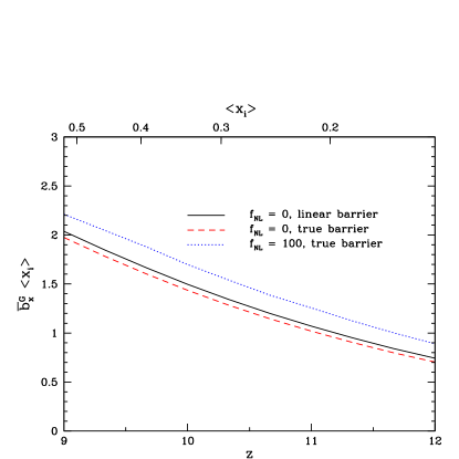
Figure 7: The volume averaged scale-independent bias.

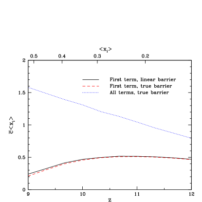
Figure 8: The volume averaged coefficient of the scale-dependent bias.

Our semi-numeric results regarding scale-dependent biasing also agree broadly with Joudaki et al. Joudaki:2011sv , who first identified the scale-dependent clustering enhancement in the ionization field. These authors approximated, however, the reionization barrier as fixed, while we further included the impact of primordial non-gaussianity on the reionization barrier itself. As a result, they did not include the scale-independent enhancement discussed here. However, we have verified that this is not a big obstacle, and that the scale-dependent signature can still be easily discerned. We expect this to be even more the case for smaller values of $f_{\rm NL}$ than considered here; given the tight constraints from Planck data, smaller values of $f_{\rm NL}\sim\pm 10$ span the currently interesting regime.

V Is it Measurable?

Now that we have characterized the impact of primordial non-gaussianity on reionization and quantified its signature in the scale-dependent clustering of ionized regions, we turn to consider whether these signatures may be observable in upcoming reionization surveys. The most promising approach is to use the scale-dependent bias, since the other effects are likely degenerate with uncertainties in the properties of the ionizing sources and the surrounding IGM. Three main types of observations have been discussed in the literature that can potentially probe or constrain the scale-dependent clustering of the ionized regions: narrow-band surveys for Ly-$\alpha$ emitting galaxies during reionization (e.g. Furlanetto:2005ir ; McQuinn:2007dy ), measurements of the small-scale CMB anisotropies induced by the patchy kinetic Sunyaev-Zel’dovich effect (e.g. Zahn:2011vp ; Mesinger:2011aa ), and measurements of the redshifted 21 cm line from the epoch of reionization (EoR) (e.g. Furlanetto:2006jb ). The latter measurement is the most direct probe of spatial fluctuations in the ionized fraction during reionization, and so we focus on these measurements here.

The main quantity of interest for the redshifted 21 cm measurements is the 21 cm brightness temperature contrast between a neutral hydrogen cloud at redshift $z$ and the CMB. We work in the limit that the spin temperature of the 21 cm line is much larger than the CMB temperature throughout all space, and further, we ignore redshift-space distortions from peculiar velocities. These are expected to be good approximations during most of the EoR (e.g. Ciardi:2003hg ; Mesinger:2010ne ; Mao:2011xp ). With these approximations, the brightness temperature contrast is:

$$T_{\rm 21}=T_{0}x_{\rm HI}(1+\delta_{\rho}).$$ (19)

The constant $T_{0}$ is $T_{0}=28\left[(1+z)/10\right]^{1/2}$ mK for our cosmological parameters Furlanetto:2006jb . Here $x_{\rm HI}$ is the neutral fraction, and $\delta_{\rho}$ is the density contrast. Each of $T_{\rm 21}$, $x_{\rm HI}$, and $\delta_{\rho}$ vary spatially and with redshift, but we have suppressed this dependence in our notation here.

The power spectrum of 21 cm brightness temperature fluctuations is related to the spatial fluctuations in the ionization field we considered earlier. If we expand to first order in fluctuations in the density contrast and to first order in neutral fraction fluctuations (neglecting redshift space distortion and spin temperature fluctuations), we expect:

$$\Delta^{2}_{\rm 21,21}(k) \approx T_{0}^{2}\left[b_{x}^{2}-2(1-\langle x_{i}\rangle)b_{x}+(1-\langle x_{i}\rangle)^{2}\right]$$ (20)

$$\times\Delta^{2}_{\delta_{\rho},\delta_{\rho}}(k).$$

Here $b_{x}$ is defined as in Equation 8: it is the linear bias factor of the ionization field, rather than the bias of the fluctuations in the ionization field that is sometimes considered. The bias factor we consider here is equal to the bias factor of the ionization fluctuations, multiplied by a factor of $\langle x_{i}\rangle$. In general, working to first order in $\delta_{x}$ can be problematic since the ionized regions are expected to be large during most of the EoR. The large spatial fluctuations in the ionization fraction imply that additional terms, dropped in Equation 20, can be important even on large spatial scales Lidz:2006vj . Since we are interested here only in the very large scale clustering signature, that applies on scales much larger than the size of the ionized regions, the approximation of Equation 20 should nonetheless be adequate. In this approximation, Equation 20 relates the bias factor of the 21 cm fluctuations to the bias factor measured in the previous section.

A challenge for measuring the scale-dependent clustering signature with future 21 cm measurements is that primordial non-gaussianity significantly impacts clustering only on rather large scales. On these large scales foreground contamination in the redshifted 21 cm data may be prohibitive. At the frequencies of interest, foreground contamination from galactic emission and extragalactic point sources is expected to have a mean brightness temperature that is roughly four orders of magnitude larger than the average redshifted 21 cm signal from the epoch of reionization. Fortunately, the foreground contamination is expected to be spectrally smooth and distinguishable from the redshifted 21 cm signal which should have significant frequency structure (e.g. McQuinn:2005hk ). Nevertheless, cleaning this contamination will prohibit measuring the signal for long wavelength modes along the line of sight, and weaken the ability to measure the large-scale power spectrum, precisely where primordial non-gaussianity should have its most pronounced effects.

The impact of foreground cleaning depends on the bandwidth over which the contamination is estimated, and the precise algorithm used to separate or subtract the slowing varying line of sight modes (e.g. McQuinn:2005hk ; 2011MNRAS.413.2103P ). One commonly discussed approach is to fit a low order polynomial in frequency to each interferometric pixel in the Fourier $(u,v)$ plane. The optimal choice for this method is to use the lowest order polynomial for which the residual foreground power is well beneath the signal power. Higher order polynomials are required to fit the foregrounds if the fitting is done over larger bandwidths. Previous work suggests that a cubic polynomial, described by $N=4$ coefficients, is adequate for fitting foregrounds over a bandwidth of $32$ Mhz Bowman:2008mk . For reference, the co-moving length scale corresponding to $32$ Mhz of bandwidth is

$$L_{\rm band}=390\,{\rm Mpc}/h\left[\frac{B}{32\,{\rm Mhz}}\right]\left[\frac{0.27}{\Omega_{\rm m}}\right]^{1/2}\left[\frac{1+z}{9}\right]^{1/2}.$$

(21)

A simple estimate is that a polynomial of order $N$ has $N-1$ nodes, and hence removing a polynomial fit of this order removes modes with line-of-sight wavenumber $|k_{\parallel,\rm min}|<N\pi/L_{\rm band}$ 2012Natur.487…70V . This suggests that the minimum measurable wavenumber, $k^{2}=k_{\parallel}^{2}+k_{\perp}^{2}$, after foreground cleaning is $k_{\rm min}=|k_{\parallel,\rm min}|=N\pi/L_{\rm band}$. If $N=4$ and $B=32$ Mhz, $k_{\rm min}=0.032h$ Mpc^-1. Comparing with Figure 6, it appears that adequate foreground cleaning will remove the Fourier modes where primordial non-gaussianity has its largest impact $k\lesssim 0.02h$ Mpc^-1. This rough estimate illustrates the challenge of detecting or constraining primordial non-gaussianity with redshifted 21 cm measurements, but more detailed calculations are required for a quantitative forecast. In particular, there may still be a ‘window’ of scales where the distinctive scale-dependent bias signature can be separated from foreground contamination.

V.1 Fisher Forecasts

In order to quantify the prospects for constraining $f_{\rm NL}$ in the presence of foreground contamination in more detail, we use the Fisher matrix formalism.

V.1.1 No foregrounds

We first consider the constraints that can be achieved in the absence of foregrounds; the effects of foreground subtraction will be dealt with below. We calculate constraints in the two-dimensional parameter space $\vec{p}=\left(f_{\rm{NL}},b_{x}^{G}\right)$, where $b_{x}^{G}$ is the gaussian bias. In general, $\langle x_{i}\rangle$ – and additional scale-independent clustering enhancement terms – might be included as additional parameters. For simplicity, we instead fix $\langle x_{i}\rangle$ and stick to this two parameter model here, since we expect variations in $b_{x}^{G}$ to be more important. The Fisher matrix is given by

$$\mathcal{F}_{\alpha\beta} = \frac{1}{2}\mathrm{Tr}\left[C_{,\alpha}C^{-1}C_{,\beta}C^{-1}\right],$$ (22)

where $C$ is the covariance matrix of the observed data, and $\alpha$, $\beta$ index the components of $\vec{p}$. The parameter covariance matrix, $C^{p}_{\alpha\beta}=\langle p_{\alpha}p_{\beta}\rangle$, (where the average is over many cosmological realizations) can then be obtained from $\mathcal{F}$, assuming gaussian statistics, by

$$\left(C^{p}\right)^{-1}=\mathcal{F},$$ (23)

where we have used the superscript $p$ to distinguish between the parameter covariance matrix and the covariance matrix of the observed data. Constraints on $f_{\rm{NL}}$ and $b_{x}^{G}$ can then be extracted from $C^{p}$ in the usual way.

To compute the covariance matrix of the observed data, $C$, we define a data vector, $\vec{\delta}$, whose components $\delta_{i}$ represent the observed 21 cm brightness temperature fluctuations in the voxels of the experiment. The data covariance matrix is related to the observable vector by $C_{ij}=\langle\delta_{i}\delta_{j}\rangle$, where again the average is over many cosmological realizations. The covariance matrix $C_{ij}$ can be written as a sum of a part due to the signal, $C_{S}$ and a part due to noise, $C_{N}$.

To simplify the calculation of the signal covariance matrix, we ignore any anisotropy of the power spectrum (due, for instance, to redshift space distortions), which should be a good approximation during most of reionization. We divide the total survey volume into sub-surveys with line of sight depth corresponding to a bandwidth of 30 MHz (as we will discuss in a moment, foreground subtraction will be performed separately in each sub-survey). For simplicity we neglect evolution across the line of sight depth of each sub-survey. Although this is an imperfect approximation, it should be adequate for our purposes since foreground cleaning removes the long wavelength modes along the line of sight where evolution should be most important. Given these assumptions, the signal covariance matrix in a single sub-survey can be written as

$$\left[C_{S}\right]_{ij} = T_{0}(z_{i})T_{0}(z_{j})\left(\frac{D(z)}{D(0)}\right)^{2}$$

$$\times\int\frac{d^{3}k}{(2\pi)^{3}}\left[P_{\delta_{\rho},\delta_{\rho}}(k)\left(b_{\rm 21}(k,z)\right)^{2}\right]\tilde{\psi}_{i}(\vec{k})\tilde{\psi}^{*}_{j}(\vec{k}),$$

where we have defined

$$b_{\rm 21}(k,z)=-b_{x}^{G}(z)-\frac{3(b_{x}^{G}(z)-1)f_{\mathrm{NL}}\Omega_{\rm m}H_{0}^{2}\delta_{B}}{c^{2}D(z)k^{2}T(k)}+(1-\langle x_{i}\rangle).$$

In this equation, $b_{\rm 21}(k,z)$ is the bias factor that converts fluctuations in the underlying density field to fluctuations in a 21-cm map. The form here follows from the term in the square brackets of Equation 20. The 21 cm bias is negative because large scale overdense regions are preferentially ionized during reionization – and consequently dim in 21 cm – while large scale underdensities remain neutral and are hence bright in 21 cm. The $T_{0}(z)$ factors are dimensionful functions that perform the unit conversions into 21-cm brightness temperature as in Equation 19. $D(z)$ is the linear growth function, $P_{\delta_{\rho},\delta_{\rho}}$ is the linear matter power spectrum at present day, and $\psi_{i}(k)$ are the Fourier transforms of the voxel window functions. Here $\delta_{B}$ is related to the reionization barrier. The precise value of $b_{x}^{G}(z)$ and $\delta_{B}$ vary with the stage of reionization (especially with $\langle x_{i}\rangle$) and the reionization model. For simplicity, we ignore redshift evolution and use fiducial values of $b_{x}^{G}(z)=1.5$, $\langle x_{i}\rangle=0.3$ and $\delta_{B}=1.0$ which are in good agreement with both the analytic and numerical results presented above.

We further assume that our voxels are spherical top hats of radius $\Delta r$. In detail, 21 cm surveys will have higher frequency resolution than angular resolution, but primordial non-gaussianity impacts only large scale fluctuations, and so the higher frequency resolution will not help here. This justifies our use of spherical voxels. This leads to

$$\tilde{\psi}_{i}(\vec{k}) = \frac{1}{(4/3)\pi(\Delta r)^{3}}\int_{|\vec{x}|<\Delta r}d^{3}xe^{-i\vec{k}\cdot(\vec{x}-\vec{x}_{i})}$$ (26)

$$= 3e^{-i\vec{k}\cdot\vec{x}_{i}}\left(\frac{j_{1}(k_{r}\Delta r)}{k_{r}\Delta r}\right),$$ (27)

where voxel $i$ is located at comoving coordinate $\vec{x}_{i}$, $k_{r}$ is the radial component of $\vec{k}$ and $j_{1}$ is the spherical Bessel function of the first kind. Substituting into Eq. V.1.1 we find

$$\left[C_{S}\right]_{ij}=9T_{0}(z_{i})T_{0}(z_{j})\left(\frac{D(z)}{D(0)}\right)^{2}\int d\ln k$$

$$\left[\frac{k^{3}}{2\pi^{2}}P_{\delta_{\rho},\delta_{\rho}}(k)\left(b_{\rm 21}(k,z)\right)^{2}\right]j_{0}\left(k|\vec{x}_{i}-\vec{x}_{j}|\right)\left(\frac{j_{1}(k\Delta r)}{k\Delta r}\right)^{2}.$$ (28)

In principle, we need to include contributions from noise, but we instead consider only $C_{s}$ here, i.e., we work in the cosmic variance limit. Presently, our main aim is to explore the fundamental limit imposed by foreground cleaning, and so it is appropriate to ignore instrumental noise here. In this limit, the normalization factor $T_{0}(z)$ drops out, and we then have all the ingredients necessary to compute $\mathcal{F}$ in the absence of foregrounds. Below we consider the effects of foreground subtraction on the Fisher matrix.

V.1.2 Effects of Foreground Subtraction

One way to incorporate the effects of foreground subtraction into the Fisher formalism is to add a large amount of noise to those modes that are affected by foreground removal (i.e. that are most contaminated by foregrounds). See McQuinn:2005hk and Liu:2011hh for related approaches. Since foregrounds are expected to be smooth along the line of sight (in the frequency direction) the modes that we consider here are low-order polynomials along the line of sight and each mode is non-zero in only a single angular pixel. In effect, this means that we are assuming the foregrounds are uncorrelated between different angular pixels (a conservative assumption). We will define $m^{a}(\vec{\theta}_{i},z_{j})$ to be the value of the $a$th mode in the $i$th angular pixel and the $j$th redshift bin. So, for instance, the constant mode in the angular pixel labeled by $\alpha$ is

$$m^{constant}(\vec{\theta}_{i},z_{j})=\begin{cases}1,&\text{for all $j$ if $i=\alpha$},\\ 0,&\text{for all $j$ if $i\neq\alpha$}.\end{cases}$$ (29)

Higher order modes correspond to higher order polynomials in $z_{j}$.

To incorporate mode subtraction into the Fisher formalism, we define a constraint matrix

$$C_{con}\left(\vec{\theta}_{i},z_{j},\vec{\theta}_{i^{\prime}},z_{j^{\prime}}\right)=\kappa\sum_{a=1}^{N_{\rm{modes}}}m^{a}(\vec{\theta}_{i},z_{j})m^{a}(\vec{\theta}_{i^{\prime}},z_{j^{\prime}}),$$

where $m^{a}_{i}$ is the value of the $a$th mode in the $i$th voxel and $\kappa$ is some large number. The data covariance matrix is then adjusted by the constraint matrix:

$$C=C_{S}+C_{con},$$ (31)

and the computation of the Fisher matrix proceeds as before.

Ref. Bowman:2008mk has suggested that foregrounds can be fit with a cubic polynomial over a bandwidth of $\sim 30$ MHz. We therefore consider the effects of foreground subtraction separately in each subsurvey. We explore the effects of foreground subtraction at this level, and also vary the number of foreground modes (using higher order polynomials) to better understand the robustness of constraints on $f_{\rm{NL}}$ to foreground subtraction.

V.1.3 Fisher Results

In order to quantify the constraints on $f_{\rm NL}$ that can be obtained in the future using the technique presented here, we consider the case of a full-sky survey that covers a frequency range from 120 Mhz to 210 Mhz. This survey covers redshifts between $z=5.8$ and $z=10.8$, centered on $\langle z\rangle=8.3$. Both the survey area and the large bandwidth of our hypothetical survey are optimistic, but this is appropriate for exploring the ultimate limits on $f_{\rm NL}$ constraints from the reionization-era 21 cm signal. As discussed above, the survey volume is divided along the line of sight into three subvolumes, each with depth 30 Mhz. We divide the survey region into voxels measuring $\frac{1}{3}^{\circ}\times\frac{1}{3}^{\circ}$ across the sky and 3 Mhz in the frequency direction. The resulting voxels are roughly cubical with side length (diameter) 50 Mpc so that our spherical voxel assumption is not a bad approximation. The effects of using finer voxelizations are explored below.

As our fiducial survey has several million voxels, the resulting covariance matrix is very large. Rather than attempt to invert this large matrix, we compute the Fisher matrix for a $5^{\circ}\times 5^{\circ}$ region (with equivalently sized voxels), and scale the resulting Fisher matrix to account for greater sky coverage. Computing the Fisher matrix in this way assumes that no information is contributed by pairs of voxels separated by more than $5^{\circ}$. This is a conservative assumption and we expect it to be a reasonable approximation. We assume that foreground removal is performed separately for each line of sight and for each of the three subvolumes of the full survey.

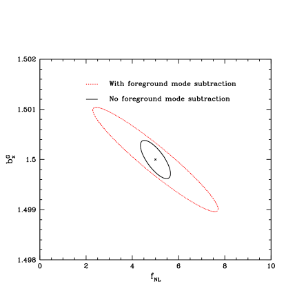
Figure 9: Fisher projections for the error on $f_{\mathrm{NL}}$ and $b_{x}^{G}$ with and without foreground mode subtraction in the two dimensional parameter space defined by $f_{\rm{NL}}$ and $b_{G}$. The cross shows our fiducial parameter values. The survey considered here is a futuristic, full-sky, cosmic-variance limited 21 cm survey covering 120-210 Mhz.

Figure 9 shows the projected constraints for the survey described above in the two dimensional parameter space defined by $\vec{p}=\left(f_{\rm{NL}},b_{x}^{G}\right)$. Fiducial values of $f_{\mathrm{NL}}$ and $b_{x}^{G}$ are marked with a cross-hair; they are $(f_{\mathrm{NL}},b_{x}^{G})=(5,1.5)$. We show both the constraints obtained in the absence of foregrounds (red, dotted curves) and those obtained when foreground subtraction is implemented in the manner described above (black, solid curve). Although the foregrounds degrade the detection, it seems that significant constraints are still reasonable even after foregrounds are subtracted. Specifically, the 1-$\sigma$ constraints on $f_{\rm NL}$ after marginalizing over $b_{x}^{G}$ are 0.43 and 1.8 before and after removing foreground contaminated modes, respectively.

To get a better sense of the range of scales that contribute most to the predicted constraint on $f_{\rm{NL}}$ in the presence of foregrounds, we now consider the effects of varying the number of voxels used in the experiment and also the number of foreground modes that are subtracted. Decreasing the number of voxels effectively decreases $k_{max}$, the maximum wavenumber used in the constraint, while increasing the number of foreground modes effectively increases $k_{min}$. Here, rather than consider an experiment across the full bandwidth, we consider one of the sub-surveys, ranging from 120 Mhz to 150 Mhz.

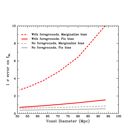
Figure 10: Fisher projections for the error on $f_{\mathrm{NL}}$ and $b_{x}^{G}$ with and without foreground mode subtraction as a function of the voxel radius of the experiment. The projections here are for a survey with 30 Mhz bandwidth rather than the 90 Mhz bandwidth assumed in Fig. 9.

Figure 10 shows the projected errors on $f_{\mathrm{NL}}$ as a function of the voxel size of the survey. In generating this figure we have assumed the same fiducial values of $f_{\rm{NL}}$ and $b_{x}^{G}$ as above: $(f_{\mathrm{NL}},b_{x}^{G})=(5,1.5)$. It is clear that the $1\sigma$ error on $f_{\rm{NL}}$ declines rapidly with decreasing voxel size until the voxel diameter is roughly 50 Mpc; little information is gained by using smaller voxels. This means that most of the information on $f_{\rm NL}$ is coming from large scales, as anticipated.

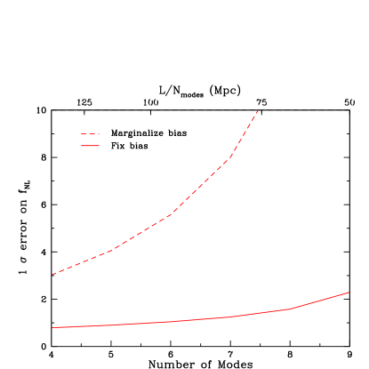
Figure 11: Fisher projections for the $1\sigma$ error on $f_{\mathrm{NL}}$ as a function of the number of foreground modes that are subtracted (over a bandwidth of 30 MHz, with 50 Mpc diameter voxels). Each foreground mode is a polynomial so that e.g. subtracting 6 modes corresponds to fitting a 5th order polynomial across the bandwidth of the experiment. Based on previous studies $N=4$ is expected to be sufficient to clean foregrounds.

We can get a handle on the maximum scale that contributes to the $f_{\rm{NL}}$ constraint after foreground cleaning by varying the number of foregrounds modes that are subtracted. Figure 11 shows the projected errors on $f_{\mathrm{NL}}$ as a function of foreground modes that we subtract across the 30 Mhz bandwidth. The upper x-axis shows the corresponding maximum scale that can be constrained by the data, given by $L/N_{\rm{modes}}$, where $N_{\rm{modes}}$ is the number of foreground modes subtracted, and $L$ is the dimension of the survey. Based on previous studies (e.g. Bowman:2008mk ), we expect $N=4$ modes to be sufficient to remove foregrounds over the bandwidth considered. Provided this is indeed sufficient, there should be a narrow range of scales that are impacted significantly by $f_{\rm NL}$, yet survive foreground cleaning. In particular, Figures 10 and 11, demonstrate that the constraint on $f_{\rm NL}$ comes mostly from the narrow range of scales between 50 Mpc to 125 Mpc, corresponding to roughly $k\sim 0.01-0.03~{}h\rm{Mpc}^{-1}$. The ability to tightly constrain $f_{\rm NL}$, in spite of this limited dynamic range in scale, is driven by the large volume of our futuristic survey. This survey samples many modes on the scales of interest and thereby provides small statistical errors on the power spectrum. It is encouraging that this may, in principle, allow constraints that are competitive with – or even slightly better than – Planck (as seen in Figure 9). The 1-$\sigma$ error in Figure 9 is $1.8$, which compares favorably to the existing 1-$\sigma$ error from Planck of $5.8$ Ade:2013ydc . However, because of foreground cleaning, the $1/(k^{2}T(k))$ signature will not be observed over a large range in scales and will imprint only a slight excess power in the largest scale modes. In effort to ensure that this signature is robust to foreground cleaning, one might test sensitivity to the number of foreground modes that are projected-out, along the lines of Figure 11.

VI Discussion and Conclusions

In this work we have investigated the effect of primordial non-gaussianity on the bias of ionized regions during reionization. We have extended the analytic model of Furlanetto et. al. Furlanetto:2004nh to the case of non-gaussian initial conditions and demonstrated that ionized regions will exhibit a scale dependent bias. Semi-numeric simulations confirm these results.

We have investigated the constraints that measurements of the power spectrum of fluctuations in the 21 cm radiation from the Epoch of Reionization may place on the gaussianity of the initial conditions. We find that futuristic redshifted 21 cm surveys might allow constraints that are competitive with Planck, in spite of foreground cleaning. This is still going to be a challenging endeavor, since interesting values of $f_{\rm NL}$ lead to only small changes in the power spectrum for the modes that survive foreground cleaning. Future galaxy surveys will also face severe systematic challenges in order to robustly measure the large scale galaxy power spectrum and constrain $f_{\rm NL}$ (e.g. Ross:2012sx ). The future prospects also need to be considered in the context of the recent Planck constraints, which almost close the door on the prospects of detecting primordial non-gaussianity, and using this to probe the physics of inflation. Nevertheless, upcoming galaxy surveys and redshifted 21 cm measurements will survey tremendous volumes, and can measure the large scale power spectrum with high statistical precision. These upcoming measurements are interesting in their own right, and will proceed regardless of searches for primordial non-gaussianity. They still deserve careful scrutiny since they should be precise enough to reveal subtle signatures from small levels of primordial non-gaussianity. Galaxy and 21 cm surveys suffer from different systematic concerns, and their combination may still provide a powerful test of primordial non-gaussianity in the post-Planck era.

- (1) P. Ade et al., “Planck 2013 Results. XXIV. Constraints on primordial non-Gaussianity,” 2013, 1303.5084.
- (2) E. Komatsu, “The pursuit of non-gaussian fluctuations in the cosmic microwave background,” 2002, astro-ph/0206039.
- (3) P. Creminelli, A. Nicolis, L. Senatore, M. Tegmark, and M. Zaldarriaga, “Limits on non-gaussianities from wmap data,” JCAP, vol. 0605, p. 004, 2006, astro-ph/0509029.
- (4) K. M. Smith, L. Senatore, and M. Zaldarriaga, “Optimal limits on fNLlocal from WMAP 5-year data,” JCAP, vol. 0909, p. 006, 2009, 0901.2572.
- (5) N. Dalal, O. Dore, D. Huterer, and A. Shirokov, “The imprints of primordial non-gaussianities on large-scale structure: scale dependent bias and abundance of virialized objects,” Phys.Rev., vol. D77, p. 123514, 2008, 0710.4560.
- (6) A. Loeb and M. Zaldarriaga, “Measuring the small - scale power spectrum of cosmic density fluctuations through 21 cm tomography prior to the epoch of structure formation,” Phys.Rev.Lett., vol. 92, p. 211301, 2004, astro-ph/0312134.
- (7) A. Cooray, “21-cm Background Anisotropies Can Discern Primordial Non-Gaussianity,” Phys.Rev.Lett., vol. 97, p. 261301, 2006, astro-ph/0610257.
- (8) S. Furlanetto, M. Zaldarriaga, and L. Hernquist, “The Growth of HII regions during reionization,” Astrophys.J., vol. 613, pp. 1–15, 2004, astro-ph/0403697.
- (9) O. Zahn, A. Lidz, M. McQuinn, S. Dutta, L. Hernquist, et al., “Simulations and Analytic Calculations of Bubble Growth During Hydrogen Reionization,” Astrophys.J., vol. 654, pp. 12–26, 2006, astro-ph/0604177.
- (10) R. Barkana and A. Loeb, “Unusually large fluctuations in the statistics of galaxy formation at high redshift,” Astrophys.J., vol. 609, pp. 474–481, 2004, astro-ph/0310338.
- (11) I. T. Iliev, G. Mellema, U.-L. Pen, H. Merz, P. R. Shapiro, et al., “Simulating cosmic reionization at large scales. 1. the geometry of reionization,” Mon.Not.Roy.Astron.Soc., vol. 369, pp. 1625–1638, 2006, astro-ph/0512187.
- (12) D. Crociani, L. Moscardini, M. Viel, and S. Matarrese, “The effects of primordial non-Gaussianity on the cosmological reionization,” Mon.Not.Roy.Astron.Soc., vol. 394, pp. 133–141, 2009, 0809.3909.
- (13) S. Joudaki, O. Dore, L. Ferramacho, M. Kaplinghat, and M. G. Santos, “Primordial non-Gaussianity from the 21 cm Power Spectrum during the Epoch of Reionization,” Phys.Rev.Lett., vol. 107, p. 131304, 2011, 1105.1773.
- (14) H. Tashiro and S. Ho, “Constraining primordial non-Gaussianity with CMB-21cm cross-correlations?,” 2012, 1205.0563.
- (15) S. Chongchitnan, “The 21cm Power Spectrum and the Shapes of Non-Gaussianity,” JCAP, vol. 1303, p. 037, 2013, 1303.4387.
- (16) M. Maggiore and A. Riotto, “The Halo mass function from excursion set theory. III. Non-Gaussian fluctuations,” Astrophys.J., vol. 717, pp. 526–541, 2010, 0903.1251.
- (17) J. Bond, S. Cole, G. Efstathiou, and N. Kaiser, “Excursion set mass functions for hierarchical Gaussian fluctuations,” Astrophys.J., vol. 379, p. 440, 1991.
- (18) S. Furlanetto, S. P. Oh, and F. Briggs, “Cosmology at Low Frequencies: The 21 cm Transition and the High-Redshift Universe,” Phys.Rept., vol. 433, pp. 181–301, 2006, astro-ph/0608032.
- (19) A. Lidz, O. Zahn, M. McQuinn, M. Zaldarriaga, and L. Hernquist, “Detecting the Rise and Fall of 21 cm Fluctuations with the Murchison Widefield Array,” Astrophys.J., vol. 680, pp. 962–974, 2008, 0711.4373.
- (20) A. H. Pawlik, J. Schaye, and E. van Scherpenzeel, “Keeping the Universe ionized: photoheating and the clumping factor of the high-redshift intergalactic medium,” MNRAS, vol. 394, pp. 1812–1824, Apr. 2009, 0807.3963.
- (21) R. Barkana and A. Loeb, “In the beginning: The First sources of light and the reionization of the Universe,” Phys.Rept., vol. 349, pp. 125–238, 2001, astro-ph/0010468.
- (22) M. Maggiore and A. Riotto, “The Halo Mass Function from Excursion Set Theory. I. Gaussian fluctuations with non-Markovian dependence on the smoothing scale,” Astrophys.J., vol. 711, pp. 907–927, 2010, 0903.1249.
- (23) M. Maggiore and A. Riotto, “The Halo mass function from excursion set theory. II. The diffusing barrier,” Astrophys.J., vol. 717, pp. 515–525, 2010, 0903.1250.
- (24) A. De Simone, M. Maggiore, and A. Riotto, “Excursion Set Theory for generic moving barriers and non-Gaussian initial conditions,” Mon.Not.Roy.Astron.Soc., vol. 412, p. 2587, 2011, 1007.1903.
- (25) A. De Simone, M. Maggiore, and A. Riotto, “Conditional Probabilities in the Excursion Set Theory. Generic Barriers and non-Gaussian Initial Conditions,” Mon.Not.Roy.Astron.Soc., vol. 418, p. 2403, 2011, 1102.0046.
- (26) A. Paranjape and R. K. Sheth, “Halo bias in the excursion set approach with correlated steps,” Mon.Not.Roy.Astron.Soc., vol. 419, p. 132, 2012, 1105.2261.
- (27) M. Musso, A. Paranjape, and R. K. Sheth, “Scale dependent halo bias in the excursion set approach,” Mon.Not.Roy.Astron.Soc., vol. 427, pp. 3145–3158, 2012, 1205.3401.
- (28) M. Musso and R. K. Sheth, “One step beyond: The excursion set approach with correlated steps,” Mon.Not.Roy.Astron.Soc., vol. 423, pp. L102–L106, 2012, 1201.3876.
- (29) G. D’Amico, M. Musso, J. Norena, and A. Paranjape, “An Improved Calculation of the Non-Gaussian Halo Mass Function,” JCAP, vol. 1102, p. 001, 2011, 1005.1203.
- (30) P. Adshead, E. J. Baxter, S. Dodelson, and A. Lidz, “Non-Gaussianity and Excursion Set Theory: Halo Bias,” Phys.Rev., vol. D86, p. 063526, 2012, 1206.3306.
- (31) A. D’Aloisio, J. Zhang, D. Jeong, and P. Shapiro, “Halo statistics in non-Gaussian cosmologies: the collapsed fraction, conditional mass function, and halo bias from the path-integral excursion set method,” 2012, 1206.3305.
- (32) D. Wands and A. Slosar, “Scale-dependent bias from primordial non-Gaussianity in general relativity,” Phys.Rev., vol. D79, p. 123507, 2009, 0902.1084.
- (33) O. Zahn, A. Mesinger, M. McQuinn, H. Trac, R. Cen, et al., “Comparison Of Reionization Models: Radiative Transfer Simulations And Approximate, Semi-Numeric Models,” 2010, 1003.3455.
- (34) C. Bennett, D. Larson, J. Weiland, N. Jarosik, G. Hinshaw, et al., “Nine-Year Wilkinson Microwave Anisotropy Probe (WMAP) Observations: Final Maps and Results,” 2012, 1212.5225.
- (35) A. D’Aloisio, J. Zhang, P. R. Shapiro and Y. Mao, “The scale-dependent signature of primordial non-Gaussianity in the large-scale structure of cosmic reionization,” arXiv:1304.6411 [astro-ph.CO].
- (36) M. Maggiore and A. Riotto, “The Halo Mass Function from Excursion Set Theory. I. Gaussian Fluctuations with Non-Markovian Dependence on the Smoothing Scale,” Astrophys. J. , vol. 711, pp. 907–927, Mar. 2010, 0903.1249.
- (37) M. Maggiore and A. Riotto, “The Halo mass function from Excursion Set Theory. II. The Diffusing Barrier,” Astrophys. J. , vol. 717, pp. 515–525, July 2010, 0903.1250.
- (38) M. Maggiore and A. Riotto, “The Halo Mass Function from Excursion Set Theory. III. Non-Gaussian Fluctuations,” Astrophys. J. , vol. 717, pp. 526–541, July 2010, 0903.1251.
- (39) M. McQuinn, S. R. Furlanetto, L. Hernquist, O. Zahn, and M. Zaldarriaga, “The Kinetic Sunyaev-Zel’dovich Effect from Reionization,” Astrophys. J. , vol. 630, pp. 643–656, Sept. 2005, arXiv:astro-ph/0504189.
- (40) S. R. Furlanetto, M. Zaldarriaga, and L. Hernquist, “The Effects of reionization on Lyman-alpha galaxy surveys,” Mon.Not.Roy.Astron.Soc., vol. 365, pp. 1012–1020, 2006, astro-ph/0507266.
- (41) M. McQuinn, L. Hernquist, M. Zaldarriaga, and S. Dutta, “Studying Reionization with Ly-alpha Emitters,” Mon.Not.Roy.Astron.Soc., vol. 381, pp. 75–96, 2007, 0704.2239.
- (42) O. Zahn, C. Reichardt, L. Shaw, A. Lidz, K. Aird, et al., “Cosmic microwave background constraints on the duration and timing of reionization from the South Pole Telescope,” 2011, 1111.6386.
- (43) A. Mesinger, M. McQuinn, and D. Spergel, “The kinetic Sunyaev-Zel’dovich signal from inhomogeneous reionization: a parameter space study,” Mon.Not.Roy.Astron.Soc., vol. 422, pp. 1403–1417, 2012, 1112.1820.
- (44) B. Ciardi and P. Madau, “Probing beyond the epoch of hydrogen reionization with 21 centimeter radiation,” Astrophys.J., vol. 596, pp. 1–8, 2003, astro-ph/0303249.
- (45) A. Mesinger, S. Furlanetto, and R. Cen, “21cmFAST: A Fast, Semi-Numerical Simulation of the High-Redshift 21-cm Signal,” 2010, 1003.3878.
- (46) Y. Mao, P. R. Shapiro, G. Mellema, I. T. Iliev, J. Koda, et al., “Redshift Space Distortion of the 21cm Background from the Epoch of Reionization I: Methodology Re-examined,” Mon.Not.Roy.Astron.Soc., vol. 422, pp. 926–954, 2012, 1104.2094.
- (47) A. Lidz, O. Zahn, M. McQuinn, M. Zaldarriaga, and S. Dutta, “Higher Order Contributions to the 21 cm Power Spectrum,” Astrophys.J., vol. 659, pp. 865–876, 2007, astro-ph/0610054.
- (48) M. McQuinn, O. Zahn, M. Zaldarriaga, L. Hernquist, and S. R. Furlanetto, “Cosmological parameter estimation using 21 cm radiation from the epoch of reionization,” Astrophys.J., vol. 653, pp. 815–830, 2006, astro-ph/0512263.
- (49) N. Petrovic and S. P. Oh, “Systematic effects of foreground removal in 21-cm surveys of reionization,” MNRAS, vol. 413, pp. 2103–2120, May 2011, 1010.4109.
- (50) J. D. Bowman, M. F. Morales, and J. N. Hewitt, “Foreground Contamination in Interferometric Measurements of the Redshifted 21 cm Power Spectrum,” Astrophys.J., vol. 695, pp. 183–199, 2009, 0807.3956.
- (51) E. Visbal, R. Barkana, A. Fialkov, D. Tseliakhovich, and C. M. Hirata, “The signature of the first stars in atomic hydrogen at redshift 20,” Nature, vol. 487, pp. 70–73, July 2012, 1201.1005.
- (52) A. Liu and M. Tegmark, “A Method for 21cm Power Spectrum Estimation in the Presence of Foregrounds,” Phys.Rev., vol. D83, p. 103006, 2011, 1103.0281.
- (53) A. J. Ross, W. J. Percival, A. Carnero, G.-b. Zhao, M. Manera, et al., “The Clustering of Galaxies in SDSS-III DR9 Baryon Oscillation Spectroscopic Survey: Constraints on Primordial Non-Gaussianity,” 2012, 1208.1491.