Nurturing Lyman Break Galaxies: Observed link between environment and spectroscopic features

Abstract

We examine the effects of magnitude, colour, and Ly$\alpha$ equivalent width (EW) on the spatial distribution of $z\sim 3$ Lyman break galaxies (LBGs) and report significant differences in the two-point auto-correlation functions. The results are obtained using samples of $\sim$10,000–57,000 LBGs from the Canada-France-Hawaii Telescope Legacy Survey Deep fields. We find that magnitude has a larger effect on the auto-correlation function amplitude on small scales ($\lesssim$1 $h^{-1}_{70}$ Mpc, the one-halo term) and that colour is more influential on large scales ($\gtrsim$1 $h^{-1}_{70}$ Mpc, the two-halo term). We find the most significant differences between auto-correlation functions for LBGs with dominant net Ly$\alpha$ EW in absorption (aLBGs) and dominant net Ly$\alpha$ EW in emission (eLBGs) determined from $\gtrsim$95% pure samples of each population using a photometric technique calibrated from $\sim$1000 spectra. The aLBG auto-correlation function has a higher two-halo amplitude than the full LBG sample and has a one-halo term departure from a power law fit near $\sim$1 $h^{-1}_{70}$ Mpc, corresponding to the virial radii of $M_{DM}\sim$10${}^{13}M_{\odot}$ dark matter haloes. In contrast, the eLBG auto-correlation function has a one-halo term departure at $\sim$0.12 $h^{-1}_{70}$ Mpc, suggesting parent haloes of $M_{DM}\sim$10${}^{11}M_{\odot}$, and a two-halo term that exhibits a curious “hump” on intermediate scales that we localize to the faintest, bluest members. The aLBG-eLBG cross-correlation function exhibits an anti-correlation component that reinforces different physical locations for a significant fraction of aLBGs and eLBGs. We introduce a “shell” model for the eLBG auto-correlation function and find that the form can be reproduced assuming a significant fraction of eLBGs have a shell-like spatial distribution. Based on the analysis of all LBG sub-samples, and considering the natural asymmetric distribution of LBGs on the colour-magnitude diagram, we conclude that aLBGs are more likely to reside in group-like environments hosting multiple luminous ($i^{\prime}<$ 26.4) LBGs whereas eLBGs are more likely to be found on group outskirts and in the field. Because Ly$\alpha$ is a tracer of several intrinsic properties, including morphology, the results presented here imply that the mechanisms behind the morphology-density relation at low redshift are in place at $z\sim 3$ and that Ly$\alpha$ EW may be a key environment diagnostic. Finally, our results show that the LBG auto-correlation function amplitude is lower than the true average as a result of the spatial anti-correlation of the spectral types. This results holds broad consequences for all auto-correlation functions measured for any population that contains members residing in different environments as the average amplitude, and hence the inferred average dark matter mass, will always be underestimated.

1 INTRODUCTION

Lyman break galaxies (LBGs) are star forming galaxies at high redshift detected by their strong ultraviolet (UV) continua and drop in flux blueward of the Lyman limit (Steidel et al., 1996). Although searches for galaxies using other selection criteria and wavelengths have been successful in finding various populations (e.g., van Dokkum et al., 2003; Daddi et al., 2004; Chapman et al., 2005), LBGs are considered to comprise the bulk of star forming galaxies at high redshift (Reddy et al., 2005; Marchesini et al., 2007).

The spatial clustering of LBGs reveal that they reside in overdense regions of the universe (e.g., Steidel et al., 1998; Foucaud et al., 2003; Adelberger et al., 2005; Cooke et al., 2006; Hildebrandt et al., 2009; Bielby et al., 2011). The clustering is typically quantified by the two-point correlation function which is observed to closely follow a power law at large scales (greater than $\sim$200 $h^{-1}_{70}$ kpc, physical), the so-called ‘two-halo’ term, that probe the separations of parent dark matter haloes. Surveys that probe the correlation function down to small scales ($\lesssim$50 $h^{-1}_{70}$ kpc, physical; Ouchi et al., 2005; Lee et al., 2006), the so-called ‘one-halo’ term, find a departure from a power law that provides insight into the distribution of luminous galaxies (or luminous sub-haloes) within parent dark matter haloes.

Relationships between the spatial distribution and magnitude of LBGs has been reported in previous surveys and indicate that more luminous LBGs are more strongly clustered (Giavalisco & Dickinson, 2001; Ouchi et al., 2004; Kashikawa et al., 2006). Here, we explore the spatial distribution of LBGs divided into independent subsets based on their magnitude, colour, and spectroscopic features and measure the two-point auto-correlation and cross-correlation functions across both the one-halo and two-halo scales.

Investigation into a relationship between clustering and spectroscopic features is motivated by (1) the trend in magnitude with Ly$\alpha$ equivalent width (EW) and the relationships between Ly$\alpha$ EW and other ultraviolet spectroscopic and morphological properties and (2) the observed relationship between Ly$\alpha$ EW and LBG pair separation. Shapley et al. (2003) examine the spectra of $\sim$800 $z\sim 3$ LBGs and find an average luminosity increase with decreasing Ly$\alpha$ EW. In addition, that work uncovers strong relationships between Ly$\alpha$ EW and other properties such as UV continua slope, star formation rate, low- and high-ionization ISM absorption line EWs, and line velocity offsets with respect to systemic redshifts (a potential outflow signature). In addition, Cooke (2009) investigate the behaviour of Ly$\alpha$ EW on the colour-magnitude diagram and find a separation and asymmetric distribution of Ly$\alpha$ EW with colour and magnitude. Red LBGs typically exhibit dominant Ly$\alpha$ in absorption and blue LBGs typically show dominant Ly$\alpha$ in emission. The bulk of luminous LBGs are redder systems exhibiting dominant Ly$\alpha$ in absorption, i.e., there are few luminous blue LBGs and fewer bright LBGs with dominant Ly$\alpha$ in emission. Faint LBGs may consist of LBGs of both types, however, spectroscopically confirmed faint LBGs are dominated by blue systems that display Ly$\alpha$ in emission.

The spectroscopic and spectroscopic/photometric close pairs studied in Cooke et al. (2010) reveal that $z\sim 3$ LBGs within $\lesssim 20$ $h^{-1}_{70}$ kpc, physical, of another LBG exhibit dominant Ly$\alpha$ in emission. This fraction decreases with increasing separation and drops to $\sim$50–60% at $\gtrsim$50 $h^{-1}_{70}$ kpc, equivalent to the fraction measured for the full $z\sim 3$ population. In addition, that work introduced trends in morphology with Ly$\alpha$ EW as interpreted from Hubble Space Telescope (HST) restframe UV images and the non-parametric analysis of Law et al. (2007). Specifically, LBGs with dominant Ly$\alpha$ in absorption are more often diffuse, extended (lower Gini coefficients), and typically exhibit multiple star forming clumps whereas LBGs with dominant Ly$\alpha$ in emission are typically compact (higher Gini coefficients) with an apparent single, typically strong, star forming component (or two). These trends are reinforced by results of Law et al. (2012) that analyse LBGs in HST restframe optical images where morphology is better understood. Consequently, an exploration of the large and small-scale correlation functions of LBGs based on Ly$\alpha$ EW, and thus their UV spectral properties and morphology, provides a powerful means to investigate the interplay between environment and galaxy properties at high redshift.

The auto-correlation function measures the clustering strength for a galaxy population which can provide the bias of luminous galaxies with respect to the underlying dark matter to infer average halo masses and, when modeled with halo occupation distribution models, can provide an estimate of the average number of luminous galaxies hosted by the parent haloes. In contrast, the cross-correlation function is sensitive to differences in the spatial distributions of two populations indicating whether or not the compared populations reside in the same physical regions of the Universe. In order to measure the correlation functions over the range of separations necessary to sample both the one- and two-halo regimes (a few kpc to tens of Mpc) in a statistically meaningful way requires large ($\gtrsim 10^{4}$), wide-field samples. Thus, examining LBGs based on their spectroscopic properties requires an equivalent number of deep spectra which is difficult to obtain using existing facilities. Instead, we apply the $z\sim 3$ LBG spectral-type selection approach of Cooke (2009, hereafter C09) to the four square-degree Deep fields of the Canada-France-Hawaii Telescope Legacy Survey (CFHTLS) images, that enables us to achieve the necessary large samples. The photometric spectral-type criteria are found to cleanly isolate two LBG subsets, one with dominant Ly$\alpha$ in absorption and the other with dominant Ly$\alpha$ in emission and their respective UV spectral properties with $\gtrsim$95% purity as determined from $\sim$1000 $z\sim 3$ spectra. Here we use $\sim$70 Keck spectra of the $z\sim 3$ LBGs used here as a confirmation of the criteria selection and purity (§2).

The magnitude, colour, and spectral type auto-correlation functions presented here unearth fundamental differences in their behaviour, with the largest effect seen for the spectral types. The spectral type cross-correlation function exhibits an anti-correlation component which indicates that a significant fraction of the two populations do not reside in similar physical locations. The results and tests presented here point to a strong connection between the observed internal properties of LBGs and external group and field environments. Our analysis helps to provide order to the complex UV morphology of LBGs and may provide links between LBG spectral properties, environment, and kinematics to be investigated in a forthcoming paper.

This paper is organised as follows. We discuss the observations in $\S\ref{obs}$ and define our $z\sim 3$ LBG galaxy selection and LBG sub-samples in $\S\ref{z3colors}$. Correlation functions and tests are presented in $\S\ref{results}$ and are analysed over the colour-magnitude diagram and by spectral type in §5, which includes a model the results. Finally, we provide a summary in $\S\ref{conc}$. All magnitudes are in the AB (Fukugita et al., 1996) magnitude system unless otherwise noted. We assume an $H=$ 70, $\Omega_{M}=$ 0.3, $\Omega_{\Lambda}=$ 0.7 cosmology. LBG separations stated in $h^{-1}_{70}$ kpc refer to physical scales and those stated in $h^{-1}_{70}$ Mpc are in comoving coordinates, unless otherwise noted.

2 OBSERVATIONS

The Deep fields of the CFHTLS are used for the photometry in this work and consist of four widely separated square-degree MegaCam pointings imaged in five filters ($u^{*}g^{\prime}r^{\prime}i^{\prime}z^{\prime}$) during the years 2003 - 2008. We combine the highest quality data (seeing $<0.75"$ FWHM) from the first four years (with consistent $i^{\prime}$-band data) and generate deep, m${}_{lim}\sim$ 27, stacked images for each of the five filters. Further details on the data reduction and stacking process can be found in Cooke et al. (2009, Supplementary Information).

Sources are detected using the SExtractor (Bertin & Arnouts, 1996) software v.2.8.6 down to the limiting magnitude of the stacked images in each field. Detections in the $i^{\prime}$-band images (restframe $\sim$1900Å) are used to define the LBG catalogues for each field. The limiting magnitudes are defined as the magnitudes in which we retrieve 50% of fake point-like ($z\sim 3$ LBG-like) sources placed in the images. We compare the results per field with the number counts of real detections per magnitude interval and find that the two methods are consistent and that SExtractor may overestimate the limiting magnitude when using 0.198 mag (5$\sigma$) uncertainties. The limiting magnitudes vary between field and filter, with $i^{\prime}$-band limiting magnitudes ranging from $i_{lim}=$ 26.4 - 26.8 mag and $u^{*}g^{\prime}r^{\prime}$ limiting magnitudes ranging from m${}_{lim}\sim$ 27.0 - 27.5 mag. As such, we refer to the full LBG sample for the four Deep fields as the “$i^{\prime}\lesssim$ 26.4” sample hereafter, as this is the limiting $i^{\prime}$-band magnitude for identifying LBGs in the shallowest field. We note that, although other fields probe to deeper $i^{\prime}$-band magnitudes, this value is representative of our $z\sim 3$ LBG sample magnitude limit because of the need for deeper imaging in the $u^{*}$ and $g^{\prime}$ filters for colour selection and for spectral-type colour-magnitude selection as described in §3.

Follow-up spectroscopy of CFHTLS $z\sim 3$ LBG colour selected sources were acquired from 24 January 2009 through 10 March 2011 using the Low Resolution Imaging Spectrometer (LRIS; Oke et al., 1995; Steidel et al., 2004, Appendix) on the Keck I telescope. These data were obtained using either the 400/3400 or the 300/5000 grism on the blue arm and the 400/8500 grating on the red arm. Seeing ranged from $\sim$0.6 - 1.1 arcsec, FWHM, and individual integrations were 1200s. Because the data were gathered in conjunction with other research, the total exposure times per multi-object slitmask ranged from $2400-8400$s.

We targeted LBGs from m${}_{r^{\prime}}\sim$ 22 - 27 and thus obtained continuum a signal-to-noise ratios (S/N) near restframe 1700Å from a S/N $\sim$ 10 to essentially non-detection for Ly$\alpha$ emitting objects. We note that $z\sim 3$ LBGs can be reliably identified in continuum spectra with a S/N of only a few from their strong UV ISM features (e.g., Steidel et al., 1998, 2003, 2004; Shapley et al., 2003; Cooke et al., 2006) and from Ly$\alpha$ emission, when present, which is detected at higher significance. All objects meet the $z\sim 3$ colour-selection criteria and the few spectra that display a single emission line but have continua too faint to reliably identify ISM absorption features, the emission is assumed here to be Ly$\alpha$.

From 178 targeted spectra, 68 have high enough continuum S/N or Ly$\alpha$ S/N for confident identification. We categorise the remaining spectra as ‘unknown’ as a result of their low S/N caused mainly by shortened total slitmask integration times due to primary science programme constraints or as a result of weather. Of the identified spectra, two are $z<$ 2 sources, two are $z\sim 3$ LBGs with evidence of AGN activity, and three are $z\sim 3$ LBGs with evidence of double Ly$\alpha$ peaks and potentially two closely spaced continua in the 2-D spectra and two flux peaks in the images (i.e., potential interactions). These seven objects were omitted from the Ly$\alpha$ EW analysis.

The spectral-type criteria, spectrophotometry, and relevant tests presented here use the larger spectroscopic dataset ($\sim$800 $z\sim 3$ LBGs) of Steidel et al. (2003, hereafter S03) and composite spectra of Shapley et al. (2003).

3 LYMAN BREAK GALAXY SELECTION

We design the colour selection criteria for the CFHTLS to identify $z\sim 3$ LBGs over the same redshift path as S03 to aid in direct comparison to the results of C09. We determine the criteria using (1) the color evolution of galaxy templates, (2) spectrophotometry using $z\sim 3$ LBG composite spectra, and (3) the identified LBG spectra in the fields.

Firstly, we convolve seven star forming, one QSO, and two early-type galaxy templates with the throughput of the $u^{*}g^{\prime}r^{\prime}i^{\prime}z^{\prime}$ filters, MegaCam detector quantum efficiency, and the atmospheric extinction of Mauna Kea and then evolve the templates from $z=$ 0–3.5 in multiple colour-colour planes. We vary the amount of absorption caused by optically thick systems in the line of sight (D_A) and include a star forming template that brackets 0.2–2.0 times the value measured for average LBGs at $z\sim 3$.

Secondly, we compute the spectrophotometric colors for four $z\sim 3$ LBG composite spectra. Shapley et al. (2003) separated 794 $z\sim 3$ LBG spectra into quartiles based on Ly$\alpha$ EW. The composite spectra are formed from these data and consist of $\sim$200 LBGs from each quartile. As such, the composite spectra reflect a consistent increase in net Ly$\alpha$ EW and decrease in reddening, ISM line widths, and star formation rates. We randomly pull from the observed redshift and $\cal{R}$ magnitude distributions for each quartile to compute $\cal{R}$-band fluxes for each composite spectrum. We perform this analysis 1000 times while measuring the corresponding flux in the $U_{n}$ and $G$ bandpasses to determine the colors for each spectrum.

Figure 1: Colour-colour plot for the data of Steidel et al. (2003). The various curves trace the colour-colour evolution of 10 galaxy templates from $z=$ 0–3.5. Star-forming templates and a QSO template are indicated by the dashed (blue) curves for $z=$ 0–2.5 and the solid (maroon) curves for $z=$ 2.5–3.5. Dotted (green) curves trace the evolution of early-type galaxies from $z=$ 0–1 (thick) and $z=$ 1–3.5 (thin) for completeness but are less reliable beyond $z\sim$ 1. The four tracks shown by the blue, green, yellow, and red crosses indicate the evolution of LBG composite spectra with decreasing Ly$\alpha$ EW, respectively, over the redshift path of the Steidel et al. (2003) sample ($z\sim$ 2.5–3.5). The $z\sim 3$ LBG colour-selection region is bounded by the thick lines. Squares denote spectroscopically confirmed LBGs.

We test our spectrophotometry in the ($U_{n}-G$) vs. ($G-\cal{R}$) color plane and on the colour-magnitude diagram (CMD). The latter is discussed in §3.1.2. These tests reveal that the composite spectra are very representative of the average spectrum in each quartile and thus accurately trace the colour-colour evolution and colour-magnitude distribution of each quartile and the full population when combined. The colour-colour evolution tracks for the composite spectra over the exact redshifts of the S03 survey, $\langle z\rangle=$ 2.96 $\pm$0.26, are traced by the crosses in Figure 1.

Confident that our spectrophotometry duplicates the $U_{n}G\cal{R}$ colour selection, we determine the colour evolution of the composite spectra when passed through the CFHTLS filters. By doing so, we are “observing” the S03 objects with the $u^{*}g^{\prime}r^{\prime}i^{\prime}z^{\prime}$ filters. Both the template evolution and composite spectrophotometry are studied in all permutations of colour-colour space, however, because the $z^{\prime}$-band data is shallower than the other bands and has accompanying larger photometric errors, we do not include these data when determining the colour-selection criteria. The colour evolution of the composite spectra and the star forming templates can be seen in the three colour-colour planes shown in Figure 2.

The general LBG colour-selection criteria shown by the dot-dash line in Figure 2 is typical of $z\sim 3$ colour selection regions designed to probe a similar redshift path as that of S03. These criteria avoid the low redshift tail for some templates and composite spectra where the density of objects in the field is high (cf. the darkest contour in each panel of Figure 2). Our spectra confirm that the colour-selection criteria are highly effective and yield the same redshift distribution as S03 (see §3.1.4). In an effort to improve the LBG purity of the colour-selection criteria, we make conservative cuts (solid lines in Figure 2) just inside the general colour-selection regions to account for photometric uncertainties that result in $\sim$0.1 mag scatter in the colour-colour plane and to further remove LBG selection from the central high density region of low redshift field objects and the regime of lower redshift reddened elliptical galaxies and the stellar locus.

We define the following selection criteria with the aim of selecting a clean sample of $\langle z\rangle=$ 3.0 $\pm$0.3 LBGs for the work presented here.

$$(u-g)>0.7$$ (1)

$$(u-g)>1.2*(g-r)+0.9$$ (2)

$$-1.0<(g-r)<1.0$$ (3)

$$(u-g)>(g-i)+0.7$$ (4)

$$-1.0<(g-i)<1.3$$ (5)

$$(r-i)<0.4$$ (6)

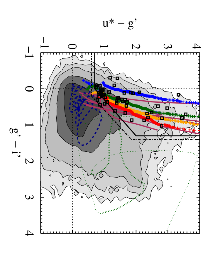
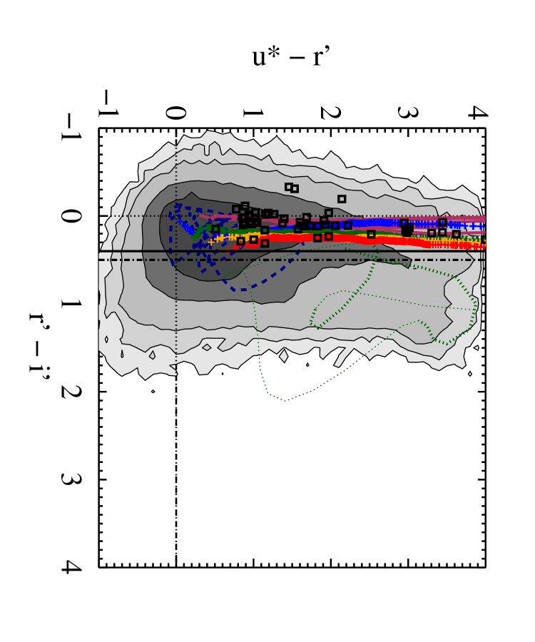
Figure 2: Colour-colour plots for the CFHTLS survey Deep fields plotted similarly to Figure 1. Grey contours trace the $\sim$2 million sources detected in the stacked images for the four square-degree fields with each level reflecting a 4$\times$ greater number density than the previous lighter shaded contour. Black solid lines mark the boundaries of the conservative colour selection regions used in this work whereas the dot-dash lines mark the regions for a more standard criteria.

Applying equations 1 - 6 to the stacked images of the four square-degree CFHTLS fields identifies 57,382 $z\sim 3$ LBGs for our m${}_{i^{\prime}}\sim$ 26.4 sample.

To further assess the efficiency of our criteria and the make-up of the selected populations, we analyse the follow-up Keck spectroscopy. We find that two of the 68 spectra (3%) are low redshift objects with colors that mimic $z\sim 3$ LBGs. This low fraction helps confirm the effectiveness of our criteria. As mentioned in §2, two objects show signs of AGN activity and this fraction is consistent with that found in the larger spectroscopic samples of S03 and Cooke et al. (2006). Finally, three objects appear to be interacting systems which is consistent with the fraction found in Cooke et al. (2010). We conclude that our criteria is highly efficient and produces samples that are representative of the full LBG population.

3.1 Lyman Break Galaxy Sub-Samples

3.1.1 Colour and Magnitude

As described in §4.2, we use simple divisions of the ($g^{\prime}-i^{\prime}$) versus $i^{\prime}$ CMD to test the effects of colour and magnitude on the various LBG ACF sub-samples. We split the CMD in half horizontally, in observed ($g^{\prime}-i^{\prime}$), to produce samples to test colour effects. Similarly, we split the CMD in half vertically, in observed $i^{\prime}$, to test magnitude effects. Below, we first detail the more complicated process to divide the CMD into regions that contain pure samples of LBG spectral types, those having different net Ly$\alpha$ EW. Finally, we test the effects of colour and magnitude on the LBG spectral type samples in §4.2.2.

3.1.2 Spectral types

LBGs display Ly$\alpha$ in absorption, emission, or a combination of both. The net Ly$\alpha$ EW distribution for LBGs at $z\sim 3$ has a wide range, from net Ly$\alpha$ EW $\lesssim$ -50Å to $\gtrsim$ 200Å, with an asymmetric peak near zero (Shapley et al., 2003). As mentioned earlier, there is a strong relationship between Ly$\alpha$ EW and other spectroscopic properties. LBGs with net Ly$\alpha$ EW in absorption show redder UV continua (see Figure 3), higher star formation rates, stronger/broader ISM absorption lines, and larger line velocity offsets with respect to systemic redshifts as compared to LBGs with net Ly$\alpha$ EW in emission. Thus, net Ly$\alpha$ EW is a direct indicator of multiple spectroscopic features and LBG properties that are directly relevant to this work.

Although Ly$\alpha$ is the dominant spectroscopic feature of LBGs, the relatively low S/N of many of the spectra affects our ability to make a precise measure of the net EW. We find that the Ly$\alpha$ forest and absorption features near Ly$\alpha$ make an accurate determination of the continuum level difficult and result in a net Ly$\alpha$ EW uncertainty of $\sim$ 25% for Ly$\alpha$ emission features and $\sim$25 - 50% for Ly$\alpha$ absorption features. Consequently, we treat our LBG spectra in a similar manner as C09. We divide the spectra into two groups with net Ly$\alpha$ EW significantly removed from net Ly$\alpha$ EW $=$ 0, relative to the uncertainties, to classify LBGs with dominant Ly$\alpha$ in absorption, termed ‘aLBGs’ and Ly$\alpha$ in emission, termed ‘eLBGs’. We adopt net Ly$\alpha$ EW $<$ -10Å for aLBGs and net Ly$\alpha$ EW $>$ 20Å for eLBGs based on the range of net Ly$\alpha$ EW for quartile 1 LBGs (strongest net Ly$\alpha$ EW in absorption) and quartile 4 LBGs (strongest net Ly$\alpha$ EW in emission) of Shapley et al. (2003) and from similar net Ly$\alpha$ EW results of our spectroscopic sample. All other LBGs are classified as “grey area” LBGs, or ‘gLBGs’, with net Ly$\alpha$ EW near zero. As a note, the Ly$\alpha$ EW cut places most eLBGs under conventional definitions of Ly$\alpha$ emitters (LAEs) detectable in deep narrow-band surveys.

3.1.3 Spectral type photometric selection criteria

C09 identifies a natural segregation of the aLBG and eLBG net Ly$\alpha$ EW distributions on the CMD and uses that property to isolate highly pure samples of the two sub-populations. The criteria were determined using the S03 data set which contains $\sim$800 $U_{n}G\cal{R}$-selected spectra. The spectral type selection technique exploits the inverse relationship between the the UV continuum near $\sim$1700Å and the combination of continuum, Ly$\alpha$ feature, and Ly$\alpha$ forest near $\sim$1200Å. As a result, using broadband information alone, $>95$% pure samples of each LBG spectral type can be confidently isolated.

The four-year stacked images of the CFHTLS Deep fields enable LBG detections over $\sim$$10\times$ the area and $\sim$1–1.5 mags deeper than the S03 survey data considered in the C09 analysis. The CFHTLS data provide the necessary large samples of the LBG spectral types to perform the first detailed study of their spatial distribution. However, to properly apply the results of C09 to the data here, we need to correct for the differences between the MegaCam and S03 filters.

The relevant filters are shown in Figure 3. The sensitivities for the CFHT $g^{\prime}$ filter (4872/1455; central wavelength/bandwidth in Å) and S03 $G$ filter (4780/1100) are similar, with the $g^{\prime}$ filter being somewhat broader and redder. The S03 $\cal{R}$ filter sensitivity (6830/1250) falls between those of the CFHT $r^{\prime}$ (6282/1219) and $i^{\prime}$ (7776/1508) filters. Because LBG continua are relatively flat over the wavelength ranges probed by the $r^{\prime}$, $\cal{R}$, and $i^{\prime}$ filters, and because of the similarity between the $g^{\prime}$ and $G$ filters, we expect the corrections to the criteria used in C09 to be relatively small. We quantify the corrections using a spectrophotometric analysis and by using the distributions of our Keck CFHTLS spectra.

Figure 3: Lyman break galaxy (LBG) spectral regions sampled by the filters studied here. Solid curves show the Steidel et al. (2003) $U_{n},G,\cal{R}$ filters and the dashed curves show the CFHTLS $u^{*},g^{\prime},r^{\prime},$ and $i^{\prime}$ filters. Overlaid are composite $z\sim 3$ LBG galaxy spectra shifted to $z=$ 3; an aLBG (dominant Ly$\alpha$ in absorption) in red and an eLBG (dominant Ly$\alpha$ in emission) in blue. Although $\cal{R}<$25.5 LBGs with dominant Ly$\alpha$ in absorption are $\sim$0.4 mag more luminous on average (Shapley et al., 2003), the templates shown here are normalised in the $\cal{R}$ filter to help illustrate the flux differences between the $G$ and $\cal{R}$ filters that segregate the spectral types on a colour-magnitude diagram. The $g^{\prime}$ and $i^{\prime}$ filters produce similar flux differences.

The spectrophotometry of the LBG composite spectra as described above accurately reproduces the magnitude and colour means and dispersions on the $G$ vs. $G-\cal{R}$ CMD for each of the four quartiles (Table 1), as well as the full CMD distribution of S03 when combined. The exception is quartile 4 containing the strongest Ly$\alpha$ emission (eLBGs) which has an offset in the colour mean by -0.12 mag. The contribution to the average Ly$\alpha$ EW from a small number of strong Ly$\alpha$ emitters results in a bias of the composite spectrum colour as compared to the entire quartile sample. Because we do not have access to the individual spectra, we were not able to directly correct for this effect. Instead we applied a +0.1 mag correction to the $g^{\prime}$-band values of the composite spectrum to counter the bias.

Regarding the correction, it is important to note three points: (1) the correction is small, (2) there is no effect on the magnitude mean or dispersion ($i^{\prime}$-band based), and (3) without the correction the eLBG mean would move in a direction away from the aLBG mean. As can be seen below, the correction provides a more conservative estimate of the true aLBG and eLBG colour distribution separations. This is because the selection of the spectral types is based on a fixed separation from the distribution means. Because the correction moves the means of the two distributions closer, the fixed separation probes further from the respective spectral type mean, resulting in purer spectral-type samples at the cost of reducing the total number of objects. We conclude that, although the colors and magnitudes of individual spectra vary within each quartile, the composite spectra can be used to compute net Ly$\alpha$ EW means and dispersions on the CMD for the purposes here in lieu of individual spectra.

We then use the composite spectra to ‘observe’ the LBGs of S03 with the MegaCam filters. We use the redshift and $\cal{R}$ magnitude distributions of the S03 data to compute the $i^{\prime}$ magnitude and ($g^{\prime}-i^{\prime}$) colour distributions for each LBG when passing the composite spectra through the $g^{\prime}$ and $i^{\prime}$ filters. We do this for the magnitude range of the S03 data and extend this $\sim$1 magnitude fainter to estimate the values for the full CFHTLS sample. The results are listed in Table 2 and shown in Figures 4 and 5. The composite spectra do a good job in duplicating the overall form of the distributions on the $i^{\prime}$ vs. ($g^{\prime}-i^{\prime}$) CMDs. The broader form of the distributions in the bluer regions of the CMDs, i.e., the small extension of bright, blue LBGs, is nearly identical to the composite spectra distribution on the $G$ vs. $G-\cal{R}$ CMD and the tests with the S03 sample informs us that the CFHTLS means and dispersions are similarly accurate.

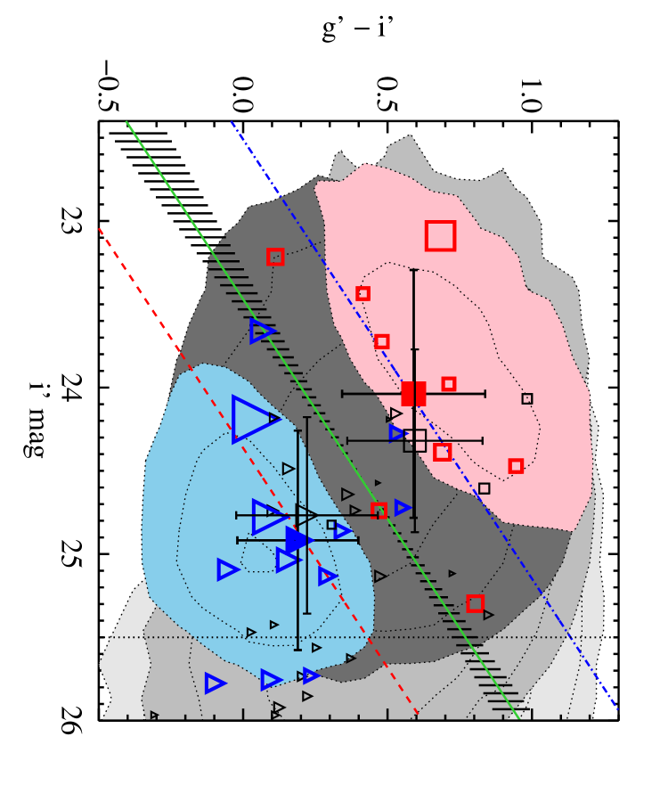
Figure 4: Colour-magnitude diagram of $z\sim 3$ Lyman break galaxy (LBG) spectral type distributions in the CFHTLS Deep fields. Shown in contours are the SExtractor 5$\sigma$ detections (light grey), the $i^{\prime}\lesssim$ 26.4 LBG sample (medium grey), and the composite spectra matched to the survey depth (m${}_{\cal{R}}\lesssim$ 25.5; vertical dotted line) of Steidel et al. (2003, dark grey). Each inner contour ridge represents 4$\times$ the number density of the previous. CFHTLS spectroscopically confirmed LBGs are shown as open squares and triangles with the symbol size reflecting the relative net Ly$\alpha$ EW strength with respect to zero such that larger squares have stronger absorption and larger triangles have stronger emission. Coloured symbols are objects that meet our aLBG/eLBG Ly$\alpha$ EW criteria whereas smaller black symbols are consistent with zero net Ly$\alpha$ EW. The error crosses with solid symbols mark the respective (m${}_{i^{\prime}}\lesssim$ 25.5) means and 1$\sigma$ dispersions of the spectra, whereas the open symbols denote the spectrophotometric means and 1$\sigma$ dispersions. The solid (green) line divides the two spectrophotometric distributions and the dashed (red) and dot-dashed (blue) lines denote $\gtrsim$2.5$\sigma$ from either distribution mean. The hatched region denotes the range of slopes from the spectra and the spectrophotometric analysis. The pink and light blue regions represent spectrophotometric $U_{n}G{\cal R}$ aLBGs and eLBGs, respectively, meeting the spectral-type criteria in Cooke (2009) transformed into the $g^{\prime}$ and $i^{\prime}$ colour-magnitude space.

Next, we compute the ($g^{\prime}-i^{\prime}$) and $i^{\prime}$ aLBG and eLBG means and dispersions for our confirmed Keck spectra. We determine the values with $i^{\prime}\lesssim$ 25.5 to compare directly with the S03 data and those for the $i^{\prime}\lesssim$ 26.4 sample. The results are listed in Table 2 and illustrated in Figures 4 and 5. The means and dispersions of the $i^{\prime}\lesssim$ 25.5 spectra and spectrophotometry are consistent, supporting the analysis of the LBG composite spectra with the CFHTLS filters.

We repeated this analysis for $z\sim 3$ LBG ($g^{\prime}-r^{\prime}$) colour and $r^{\prime}$ magnitude distributions. The results of this investigation show that, as expected from the wavelengths probed by each of the filters, the aLBG and eLBG ($g^{\prime}-r^{\prime}$) and $r^{\prime}$ distributions are closer together on the CMD and have more overlap than distributions using $G$ and $\cal{R}$ or $g^{\prime}$ and $i^{\prime}$ filters. LBG spectral types are separated in part by the slope of their continua longward of restframe $\sim$$1500$Å, with increasing differences with increasing wavelength (cf. Figure 3). As such, we find that the larger differences provided by the $g^{\prime}$ and $i^{\prime}$ filters are more effective in separating the distributions on the CMD as compared to the $g^{\prime}$ and $r^{\prime}$ filters for the redshift path probed.

For the $i^{\prime}\lesssim$ 25.5 sample, we follow the spectral-type approach of C09 and define a primary cut that statistically divides the two distributions (solid green line in Figure 4). The aLBG region is then determined as the area to the upper left of (brighter and redder than) a line placed 1.5$\sigma$ redward of the primary cut, away from the eLBG distribution mean, with the same slope. Similarly, the eLBG spectral-type region is the area to the lower right of (fainter and bluer than) a line placed $\sim$1.5$\sigma$ away from the primary cut and blueward of the aLBG distribution mean. As a result, each spectral type region is $\gtrsim$2.5$\sigma$ (2.5$\sigma$ at its closest) from the other spectral type distribution mean. The number of aLBG and eLBG Keck spectra is relatively small to accurately determine the slope of the primary cut alone but yield means and dispersions similar to the spectrophotometric values. Because the position and slope of the primary cut from the spectrophotometric analysis is similar to that determined by the spectra (hatched region in Figure 4), we use the average of the two values.

Redshift identifications and Ly$\alpha$ EW measurements of faint, $i^{\prime}\gtrsim$ 25.5 spectra can only be efficiently determined for LBGs with Ly$\alpha$ in emission, therefore we only estimate the $i^{\prime}\gtrsim$ 25.5 eLBG distribution. Although we have identified objects with dominant Ly$\alpha$ emission to $i^{\prime}\sim$ 27, interestingly, we find none in the region bounded by $i^{\prime}\gtrsim$ 25.5 and $(g^{\prime}-i^{\prime})>$ 0.5. Given that LBGs meeting the colour-selection criteria are detected with $i^{\prime}\gtrsim$ 25.5 and $(g^{\prime}-i^{\prime})>$ 0.5, the region contains either (1) aLBGs with a similar level of purity as the $i^{\prime}\lesssim$ 25.5 sample (i.e., no change in color with magnitude), (2) LBGs with net Ly$\alpha$ EW $\sim$ 0 (i.e., gLBGs) only, or (3) a combination of the two. The $i^{\prime}\lesssim$ 26.4 spectrophotometric analysis makes no assumptions of a colour trend for $i^{\prime}\sim$ 25.5–26.4 objects and therefore the distributions differ from the $i^{\prime}\lesssim$ 25.5 distributions in magnitude only. As a result, the spectrophotometric aLBG analysis provides an estimate of scenario (1). Because we are not able to confidently identify our $i^{\prime}\gtrsim$ 25.5 spectra as aLBGs, and the lack of eLBGs, results in the $i^{\prime}\lesssim$ 26.4 aLBG mean being unaffected from the $i^{\prime}\lesssim$ 25.5 value, thus providing an estimate of scenario (2). As a result, the two colour and magnitude mean and distribution estimates bracket the range of values for the $i^{\prime}\lesssim$ 26.4 aLBG sample for all three scenarios.

Table 1:

Colour and magnitude means and dispersions Spectral type^a $G-\cal{R}$ $G-\cal{R}$ $\cal{R}$ mag $\cal{R}$ mag $\cal{R}$ mag mean 1$\sigma$ mean 1$\sigma$ limit^b S03 q1 data 0.75 0.25 24.44 0.53 25.5 S03 q1 composite 0.77 0.25 24.44 0.55 25.5 S03 q2 data 0.68 0.26 24.51 0.50 25.5 S03 q2 composite 0.70 0.25 24.52 0.52 25.5 S03 q3 data 0.60 0.25 24.68 0.52 25.5 S03 q3 composite 0.60 0.25 24.68 0.53 25.5 S03 q4 data 0.45 0.30 24.84 0.58 25.5 S03 q4 composite 0.33 0.29 24.85 0.59 25.5

^aq1 - q4 are abbreviations for quartiles 1 - 4 of Shapley et al. (2003) ^bOne field (of 17) has a limiting magnitude of $\cal{R}\sim$ 26.0 and is accounted for in the composite spectrum analysis.

Increasing the 1.5$\sigma$ displacement from the $i^{\prime}\lesssim$ 25.5 primary cut to 2.0$\sigma$ is expected to produce pure $i^{\prime}\lesssim$ 26.4 samples while considering all three scenarios and the uncertainty of the full census of $i^{\prime}\gtrsim$ 25.5 LBGs. For aLBGs, the increase to 2.0$\sigma$ avoids including gLBGs and the tail of the eLBG distribution but sacrifices the total number of aLBGs. For eLBGs, a 2.0$\sigma$ displacement similarly helps to omit the far tail of the aLBG distribution and simply avoids the $i^{\prime}\gtrsim$ 25.5 and $(g^{\prime}-i^{\prime})>$ 0.5 region over the extent of our $i^{\prime}\lesssim$ 26.4 sample.

The choice of a 2.0$\sigma$ cut comes at the cost of the total number of aLBGs and eLBGs used for our correlation function analysis, but the large numbers available from the four CFHTLS fields gives us the option to attack this problem conservatively. We vary the spectral type cut parameters (slope and displacement) over a practical range and find that there is no significant change in the overall behavior of the correlation functions of the two spectral types. Thus, the main results of this paper are insensitive to moderate departures from the spectral-type criteria defined below.

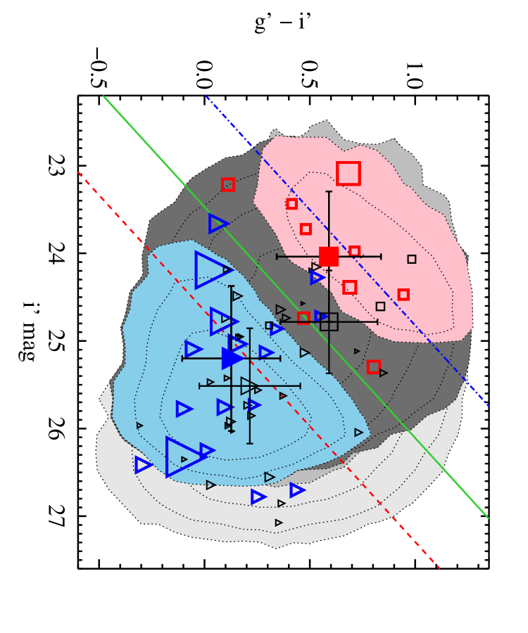
Figure 5: Similar to Figure 4, but reflecting the $i^{\prime}\lesssim$ 26.4 spectrophotometric analysis to match our higher significance sample (medium grey). The blue dot-dashed and red dashed lines define the conservative spectra-type cuts used here (see text). The cuts provide highly pure samples of each spectral type such that $\gtrsim$95% of eLBGs are below the blue dot-dashed line and $\gtrsim$95% of aLBGs are above the red dashed line.

We define the $i^{\prime}\lesssim$ 26.4 sample spectral-type criteria as

$$\mbox{aLBGs: }~{}(g^{\prime}-i^{\prime})\geq 0.38\cdot i^{\prime}-8.9+2.0\sigma_{E}$$ (7)

$$\mbox{eLBGs: }~{}(g^{\prime}-i^{\prime})\leq 0.38\cdot i^{\prime}-8.9-2.0\sigma_{A}$$ (8)

where $\sigma_{E}$=0.25 and $\sigma_{A}$=0.23 and refer to the colour dispersions for the eLBG and aLBG distributions, respectively. Note that the eLBG distribution ($\sigma_{E}$) is used to determine the aLBG spectral-type cut and vice-versa. In §4.2, we present the results from tests of other LBG sub-samples that provide insight into the effects caused by the choice of more general slope and sample criteria and the dependence of the correlation function on colour and magnitude.

Applying the spectral-type criteria to the $i^{\prime}<$ 26.4 sample in the four CFHTLS Deep fields produces 9648 aLBGs and 11567 eLBGs. Objects in the aLBG region reside $\sim 2\sigma$ from the primary cut and $\gtrsim$3.0$\sigma$ from the eLBG distribution mean and vice-versa for the objects in the eLBG region. The spectrophotometric analysis finds 3% eLBG contamination in the aLBG sample and 1% aLBG contamination in the eLBG sample. Moreover, there is zero contamination of the Keck spectra in either samples.

All LBGs that do not meet these criteria, i.e., those in-between the two cuts forming a swath through the middle of the CMD, are classified as gLBGs, formally defined as

$$\begin{split}\mbox{gLBGs: }~{}(g^{\prime}-i^{\prime})\leq 0.38\cdot i^{\prime}-8.9+2.0\sigma_{E}\\ \mbox{and}~{}(g^{\prime}-i^{\prime})\geq 0.38\cdot i^{\prime}-8.9-2.0\sigma_{A}\end{split}$$ (9)

where $\sigma_{E}$ and $\sigma_{A}$ are as defined in equations 7 and 8. These objects are comprised of a blend of aLBGs and eLBGs, with a large fraction consisting of LBGs with net Ly$\alpha$ EW $\sim$ 0. We also study this population for completeness and for added insight into the behaviour of the aLBG and eLBG correlation functions. Finally, we note that no spectroscopically confirmed aLBGs are found in either the $(g^{\prime}-i^{\prime})$ versus $i^{\prime}$ eLBG region or the equivalent ($G-\cal{R}$) versus $\cal{R}$ eLBG region using a 2.0$\sigma$ cut for the CFHTLS Keck spectra or the larger S03 spectroscopic sample. These highly pure eLBG samples reinforce the use of simple broadband criteria as an efficient means to amass large numbers of $z\sim 3$ LAEs and Ly$\alpha$ absorbers (LAAs) quickly and inexpensively, relative to conventional narrow-band or blind spectroscopic surveys.

Table 2:

CFHTLS colour and magnitude means and dispersions Type $g^{\prime}-i^{\prime}$ $g^{\prime}-i^{\prime}$ $i^{\prime}$ mag $i^{\prime}$ mag $i^{\prime}$ mag mean 1$\sigma$ mean 1$\sigma$ limit^a aLBG data 0.59 0.25 24.04 0.74 25.5 aLBG sim. 0.59 0.23 24.32 0.55 25.5 eLBG data 0.19 0.21 24.92 0.66 25.5 eLBG sim. 0.22 0.24 24.76 0.59 25.5 aLBG data 0.59 0.25 24.04 0.74 26.4 aLBG sim. 0.59 0.23 24.78 0.58 26.4 eLBG data 0.13 0.23 25.20 0.83 26.4 eLBG sim. 0.20 0.24 25.49 0.66 26.4

^aApproximate (see text). The magnitude limit of the CFHTLS $i^{\prime}\lesssim$ 26.4 sample is only relevant to eLBGs.

3.1.4 Redshift Distributions

As discussed above, our CFHTLS $z\sim 3$ LBG colour selection criteria was designed to probe the same redshift path as the S03 $U_{n}G\cal{R}$ colour-selection criteria. S03 reports $\langle z\rangle$ = 2.96, $\sigma$ = 0.29 and we find $\langle z\rangle$ = 2.99, $\sigma$ = 0.28 for our $i^{\prime}\lesssim$ 25.5 spectra and $\langle z\rangle$ = 2.97, $\sigma$ = 0.31 for the full sample. Similar to the C09 results, we find a difference in the aLBG and eLBG redshift distributions as a consequence of the separation of the two samples on the CMD. The difference occurs because higher redshift objects produce larger ($g^{\prime}$ - $i^{\prime}$) values and a standard candle is fainter by $\sim$0.6 mag when redshifted from $z=$ 2.5 to $z=$ 3.5. However the situation becomes more complicated as aLBGs are offset in colour (redder) as compared to eLBGs for a given redshift and the values have considerable scatter. In C09, we find redshift distributions $\langle z\rangle=3.05,\sigma=0.25$ and $\langle z\rangle=2.88,\sigma=0.24$, respectively, for the S03 aLBGs and eLBGs used in that analysis. Only a few of our Keck spectra meet the $i^{\prime}\lesssim$ 25.5 aLBG and eLBG criteria to estimate the CFHTLS redshift distributions, but the data appear to have a similar behaviour with $\langle z\rangle=3.05,\sigma=0.18$ (aLBG) and $\langle z\rangle=2.82,\sigma=0.23$ (eLBG) for the 1.5$\sigma$ cut. The redshift distributions for the C09 analysis and the CFHTLS data are shown in the upper panel of Figure 6.

We find similar distributions for the $i^{\prime}\sim$ 26.4 spectra meeting aLBG and eLBG criteria using the 2$\sigma$ cuts. However, more relevant to this work are the redshift distributions of all objects in the aLBG and eLBG regions, i.e., those with no net Ly$\alpha$ EW constraints, since all objects in these regions are used to compute the spectral-type correlation functions. From the Keck spectra, we find $\langle z\rangle=3.18,\sigma=0.23$ for all objects in the aLBG region regardless of spectral type and $\langle z\rangle=2.86,\sigma=0.33$ for all objects in the eLBG region. In addition, we find a redshift distribution $\langle z\rangle=3.00,\sigma=0.28$ for the gLBG sample. Redshift histograms for the three sub-samples are shown in the lower panel of Figure 6. Overlaid are Gaussian fits to the distributions normalised to the total number of objects in each sample.

Figure 6: Lyman break galaxy spectral type redshift distributions. Upper panel: The dashed (blue) and solid (red) empty histograms indicate the eLBG and aLBG redshift distributions, respectively, for the $U_{n}G\cal{R}$-selected, $\cal{R}\lesssim$ 25.5, data set of Steidel et al. (2003) as analysed in Cooke (2009). Overlaid are the eLBG and aLBG redshifts of the CFHTLS $u^{*}g^{\prime}r^{\prime}i^{\prime}$-selected, $i^{\prime}\lesssim$ 25.5 spectra denoted by the backward hatch (blue) and forward hatch (red) histograms, respectively. Lower panel: The redshift distributions for all spectra (no net Ly$\alpha$ EW restrictions) that meet the $i^{\prime}\lesssim$ 26.4 aLBG (red forward hatch), eLBG (blue backward hatch), and gLBG (grey horizontal hatch) spectral-type selection. In each panel, Gaussian fits to the redshift distributions normalised to the relative total number of objects in each sample are shown by the solid curves.

Although the two spectral-type samples have a mean redshift offsets, they have significant redshift overlap, important to the cross-correlation function results. Fitting Gaussian functions to the two distributions in C09 finds $\sim$73% overlap and similar overall redshift ranges. A similar result is found for the small number of CFHTLS $i^{\prime}\lesssim$ 25.5 spectra.

The fainter spectra in the CFHTLS $i\lesssim$ 26.4 sample favor confirmation of eLBGs given the observational program constraints (§2). Gaussian fits to the spectra in hand suggest a $\sim$53% redshift distribution overlap. The overlapping redshift path appears to be largely dictated by the aLBG redshift range, roughly 2.5 $\lesssim z\lesssim$ 3.8. It is important to note that poorer representation for a given redshift, i.e., the tails of the distributions, results only in noisier data but does not affect the amplitude of the cross-correlation function for a given $\Delta z$.

We note that the spectra from different populations need only probe the same redshift paths for the cross-correlation function to be representative of the commonality of their spatial distribution. The random catalogs in the correlation functions help to minimise the effect of projected pairs and the random projections of similar-sized clustered regions should introduce a similar bias on all separation scales. The redshift path probed by our colour selection ($\sim$2.5–3.5) secures that the clustering scales are the same. The four square-degree fields of the CFHTLS include a large number of LBG clustered regions to evenly distribute clustered regions on all scales. We explore the effect of redshift on the correlation functions in more detail in §4.2.

4 CORRELATION FUNCTIONS

We compute the correlation functions on a field-by-field basis using the auto-correlation function estimator $\omega(\theta)=(DD-2DR+RR)/RR$ (Landy & Szalay, 1993) and the corresponding cross-correlation estimator $\omega_{1,2}(\theta)=(D_{1}D_{2}-D_{1}R_{2}-D_{2}R_{1}+R_{1}R_{2})/R_{1}R_{2}$, where $DD$, $DR$, and $RR$ are the data-data, data-random, and random-random galaxy separations catalogues and the subscripts in the cross-correlation estimator refer to the two sub-samples. Random catalogues are constructed to match the field dimensions probed by the data with bright stars masked out and number densities several times the observed values and normalised. The correlation functions are determined from the average of $100$ realizations and the uncertainties are determined using $100$ jackknife error realizations, each omitting a different $1/100$th the field area. We determine the integral constraint, IC, using the approach detailed in Lee et al. (2006) and apply a value of IC = 0.012 to the data. The final results average the values for the four CFHTLS fields. Finally, we note that the square-degree fields of the CFHTLS probe well beyond the $z\sim 3$ LBG clustering correlation length ($\sim$4 $h^{-1}_{70}$ Mpc) and the multiple fields help to minimise the effect of cosmic variance.

Figure 7 presents the auto-correlation function (ACF) for the full CFHTLS $z\sim 3$ LBG sample. The $z\sim 3$ LBG ACF of Adelberger et al. (2005) derived from the $17$ smaller fields of S03 and the $z\sim 4$ results of Ouchi et al. (2005) are overlaid for comparison. We fit a power law of the form $\omega(\theta)=A\theta^{\gamma}$ to the well-sampled two-halo regime of the ACF from $\sim$1–20 $h^{-1}_{70}$ Mpc, yielding $\gamma=$ -0.612 and consistent with values given in the literature. The ACF departs monotonically from a power law at $\sim$0.12 $h^{-1}_{70}$ Mpc, comoving, similar to that found at $z\sim 4$ by Ouchi et al. (2005) probing galaxies with similar luminosities and over similar scales. The departure occurs near the viral radius for $\sim$10${}^{11}M_{\odot}$ dark matter haloes at $z\sim 3$ and is interpreted to be caused by multiple luminous sub-halo galaxies within the parent dark matter haloes and/or an effect of galaxy luminosity enhancement as a result of interactions (Ouchi et al., 2005; Berrier & Cooke, 2012).

Figure 7: LBG angular correlation functions (ACFs). The CFHTLS $z\sim 3$ LBG ACF from this work is shown as filled circles. For comparison, the $z\sim 3$ LBG ACF from Adelberger et al. (2005) and $z\sim 4$ LBG ACF from Ouchi et al. (2005, scaled to $z\sim 3$) are overlaid. The solid line is a power law fit to the CFHTLS ACF between $\sim$1–20 $h^{-1}_{70}$ Mpc separations, comoving. The ACF shows a departure from a power law at small scales ($\sim$0.12 $h^{-1}_{70}$ Mpc, comoving), a regime that probes individual dark matter haloes (the one-halo term). The two smallest bins for our data (hollow circles) and the data of Ouchi et al. (2005) (hollow squares) are potentially subject to image deblending effects.

4.1 Spectral Type Correlation Functions

In this section, we present the ACFs and cross-correlation functions (CCFs) for the spectral-type subsets. The aLBG, eLBG, and gLBG ACFs are computed as described above and shown in Figure 8 along with the full LBG ACF for comparison. We omit the two smallest bins where close galaxy pairs can be difficult to separate as a result of the seeing and SExtractor deconvolution. In addition, we compute the virial radii of $10^{10-14}M_{\odot}$ dark matter haloes using R${}_{VIR}=[(G\cdot M_{VIR})/(100\cdot H^{2}(z)]^{1/3}$ (e.g., Ferguson et al., 2004) and plot the values on Figure 8 for reference. Here, we only point out the salient features and provide a more extended examination of all ACFs features in §5. We defer a more detailed analysis of the individual correlation functions to a future paper.

The two main features of the aLBG ACF that stand out from the full LBG ACF is stronger one-halo term amplitude that extends to $\sim$1 $h^{-1}_{70}$ Mpc, comoving, ($\sim$200 kpc, physical) and the higher clustering amplitude on large scales. The strong and extended small-scale clustering reflects more massive parent dark matter haloes and multiple detected luminous (m${}_{i^{\prime}}<$ 26.4) galaxies having equal and larger separations per parent dark matter halo on average as compared to the LBG ACF. The one-halo term break in the aLBG ACF corresponds to the virial radii of $\sim$10${}^{13}M_{\odot}$ parent haloes at $z\sim 3$ and is consistent with the higher large-scale clustering amplitude.

In contrast, the eLBG and gLBG ACFs show one-halo term breaks at $\sim$120 $h^{-1}_{70}$ Mpc, comoving ($\sim$30 kpc, physical), on the same scale as the full LBG sample, and imply parent halo masses of $\sim$10${}^{11}M_{\odot}$. In fact, the gLBG ACF closely follows the full LBG ACF on all scales. Although the eLBG ACF traces the LBG ACF reasonably well, we see an enhancement, or ‘hump’ in the eLBG ACF on intermediate scales, $\sim$0.5–5 $h^{-1}_{70}$ Mpc.

We note that the LBG subset ACFs show an equivalent, or higher, amplitude than the full LBG ACF and, thus, the average LBG ACF (the combination of the three subsets) is less than the sum of its parts. This result has important implications on the values determined via correlation function measurements for potentially all galaxy populations. We explore the cause of this effect further via the spectral type CCFs below and in §5.

Figure 9 presents the aLBG–eLBG, gLBG–aLBG, and gLBG–eLBG CCFs. Bin values of the CCF amplitude that are weaker than the corresponding ACFs represent an anti-correlation and indicate different physical spatial distributions. An anti-correlation occurs when some fraction of one population does not reside in the same region of the Universe as the other, such as a location preference for groups and clusters as opposed to the field and/or as a result of non-overlapping redshift paths. The aLBG–eLBG CCF exhibits some level of anti-correlation at all scales, except the largest separation bins, and has negative values for three bins within the one-halo regime (denoted by the arrows in Figure 9). In contrast, the gLBG–aLBG and gLBG–eLBG CCFs show no anti-correlation. Both CCFs follow the gLBG ACF and the full LBG ACF within the uncertainties.

The spectral type criteria defined in this work are devised to generate sub-samples containing a high purity of aLBGs and eLBGs at the cost of containing all aLBGs and eLBGs. As a result, the aLBG and eLBG distributions extend into the gLBG region as is witnessed by our Keck spectra. However, for the gLBG–aLBG CCF (gLBG–eLBG CCF) to show no appreciable anti-correlation implies that the fraction of eLBGs (aLBGs) in the gLBG region that meet our criteria is relatively small as compared to the whole and that gLBGs (net Ly$\alpha$ EW $\sim$ 0) are found in all environments.

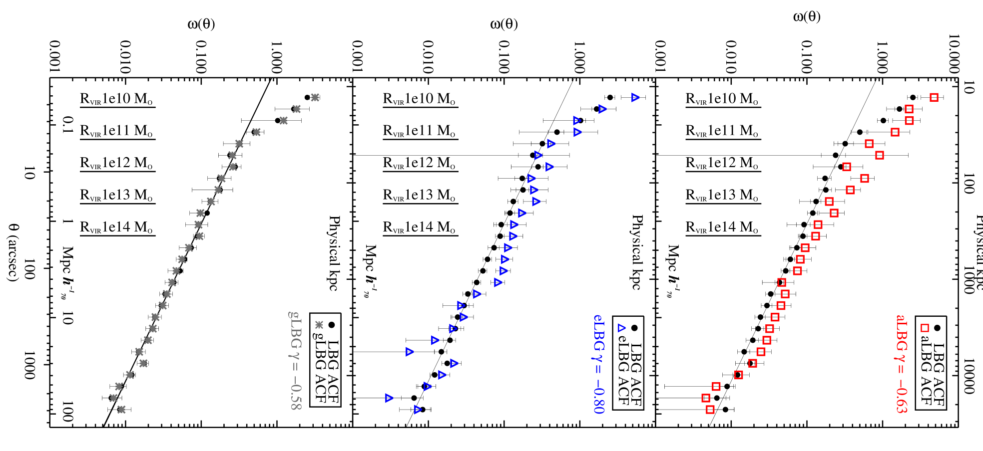
Figure 8: Auto-correlation functions (ACFs) of CFHTLS Deep field LBGs spectral-type sub-samples. The ACF for the full LBG sample (filled circles) is shown in each plot for comparison. The solid line denotes the power law fit to the full LBG ACF (see text and Figure 7). The virial radii, R_VIR, for $10^{10-14}M_{\odot}$ haloes are indicated by the short vertical lines and are labelled accordingly. The slope ($\gamma$) for the power law fit to the spectral type ACFs from $\sim$1–20 $h^{-1}_{70}$ Mpc is denoted below each legend. Upper panel: The aLBG ACF departs from a power law near $\sim$1 $h^{-1}_{70}$ Mpc, comoving, and displays a higher amplitude than the full LBG population on all scales. Center panel: The eLBG ACF behaves similar to the full LBG ACF and shows a potential higher amplitude on intermediate scales ($\sim$0.5–5 /Mpc). Bottom panel: The gLBG ACF closely follows the full LBG ACF.

Figure 9: Cross-correlation functions (CCFs) plotted similarly to Figure 8. Upper panel: The aLBG–eLBG CCF (diamonds) with the aLBG ACF (squares), eLBG ACF (triangles), and LBG ACF (solid circles) overlaid without errors for clarity. The CCF exhibits an anti-correlation (an amplitude less than the aLBG and eLBG ACF) indicating that a significant fraction of the two populations have different physical spatial distributions. Negative values for the CCF are indicated with arrows. Lower panel: The gLBG–aLBG CCF (squares) and gLBG–eLBG CCF (triangles) with the gLBG ACF (asterisks) and full LBG ACF (filled circles) are overlaid without errors for clarity. The gLBG–aLBG and gLBG–eLBG CCF do not show an appreciable anti-correlation and follow the behaviour of the full LBG population.

4.2 Magnitude and Colour Correlation Functions

One of the main objectives of this work is to examine the behaviour of LBG sub-sample ACFs based on their spectral type as is motivated by the observed relationships between Ly$\alpha$ and other LBG properties. As discussed above, the spectral type primary cut makes a diagonal slice through the CMD that statistically splits the peaks of the aLBG and eLBG distributions. Hence, each spectral type includes the effects of both magnitude and colour. However, it is equally important, and highly informative, to examine any effect that magnitude and colour make on the behaviour of LBG ACFs and to test the effects of different CMD primary cut slopes. Here, we divide LBGs into sub-samples in magnitude and colour to investigate the fundamental drivers behind various ACF features and, in a coarse sense, the colour and/or magnitude contribution to the observed differences in the aLBG and eLBG ACFs.

4.2.1 Split magnitude and colour correlation functions

As a general examination of the effect that magnitude and colour may have on the correlation functions, we divide the $(g^{\prime}-i^{\prime})$ vs. $i^{\prime}$ CMD in half at the mean magnitude of the $i^{\prime}<$ 26.4 LBG sample. In this manner, we generate “split mag” catalogues containing objects from the brightest and faintest half of the full LBG sample to directly test any magnitude effect with a simple non-biased cut. Similarly, we divide the CMD into “split colour” catalogues containing the reddest and bluest halves of the CMD based on the mean colour of the full sample. We compute the ACFs and CCFs for the “split” catalogues and present the results in Figure 10. The sample sizes are large and the correlation functions can be determined to high accuracy. However, each sample contains varying fractions of each spectral type and, in particular, are dominated in number by gLBGs that may dilute the contributions from aLBGs and eLBGs.

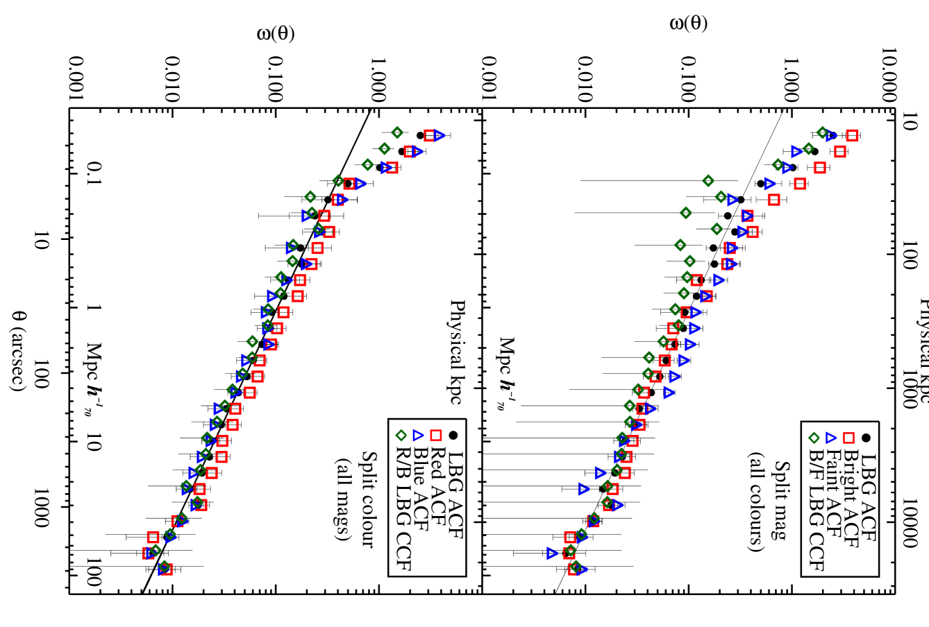
Figure 10: Auto-correlation functions (ACFs) and cross-correlation functions (CCFs) using split magnitude and split colour samples that divide the CMD in half (see text) plotted similarly to Figures 8 & 9. The large catalogues enable accurate correlation functions but contain mixed fractions of the different spectral types. Upper panel: The split magnitude ‘Bright’ and ‘Faint’ LBG ACFs. The ‘Bright’ ACF shows a strong one-halo term amplitude but roughly agrees with the full LBG ACF over the two-halo regime whereas the ‘Faint’ ACF behaves more like the eLBG ACF (see Figure 8) and exhibits a similar enhancement, or “hump”, around $\sim$0.5–5 $h^{-1}_{70}$ Mpc. The ‘Bright–Faint’ CCF shows a small anti-correlation component that is more significant at intermediate and small scales. Lower panel: The split color ‘Red’ and ‘Blue’ LBG ACFs. Both ACFs show similar behaviour and are nearly identical to the full LBG ACF. However, the ‘Red’ ACF is consistently higher than the ‘Blue’ ACF over intermediate to large scales. Neither ACF exhibits the eLBG ACF-like “hump”. The ‘Red–Blue’ CCF indicates that the two samples largely co-exist in space, but shows a anti-correlation component on small scales.

The mean magnitude of the $i^{\prime}<$ 26.4 sample is $i^{\prime}=$ 25.10$\pm 0.10$, 1$\sigma$ field-to-field scatter. When reviewing the CMD, we see that the split magnitude brighter half, or ‘Bright’ LBG sample, contains essentially all of the aLBGs, half of the gLBGs (blue and bright), and the brightest eLBGs. The ‘Bright’ ACF shows an enhancement in amplitude over the one-halo term corresponding to haloes of $M_{DM}\sim$10${}^{12}M_{\odot}$, but weakens to the roughly the amplitude of the full LBG ACF at larger separations. The split magnitude fainter half, or ‘Faint’ LBG sample, contains essentially no aLBGs, half of the gLBGs (red and faint), and essentially all eLBGs. The ‘Faint’ ACF follows the full LBG ACF at small scales but then follows the behaviour of the eLBG ACF at intermediate and large scales, similarly exhibiting a “hump” around $\sim$0.5–5 $h^{-1}_{70}$ Mpc. Although the ‘Bright’ ACF follows the full LBG ACF at large scales, interestingly, it is weakest over the range of the “hump”.

The ‘Bright–Faint’ CCF shows a level of anti-correlation, especially near the elbow of the one-halo, two-halo terms. The strongest anti-correlation coincides with the range of separations in which the aLBG ACF maintains an enhancement over the ‘Bright’ ACF. In addition, the ‘Bright’ and ‘Faint’ LBG samples are quite heterogeneous and a sufficient fraction of aLBGs and eLBGs, and their extremes, in the two samples may exist to produce a net anti-correlation.

The mean colour for the $i^{\prime}<$ 26.4 LBG sample is $(g^{\prime}-i^{\prime})=$ 0.54$\pm$0.01. Thus, the split color redder half, or the ‘Red’ LBG sample, contains the bulk of the aLBGs (the reddest), half of the gLBGs (red and faint), and essentially no eLBGs. The split color bluer half, or the ‘Blue’ LBG sample, contains a small fraction of aLBGs (the brightest and bluest), half of the gLBGs (blue and bright), and essentially all of the eLBGs. The ‘Blue’ LBG sample contains fewer bright objects as compared to the ‘Red’ LBG sample, as seen in the natural CMD asymmetry. The ACFs for both samples closely follow the full LBG ACF, with the two-halo term amplitude of the ‘Red’ ACF consistently higher than full LBG ACF and the ‘Blue’ ACF similar to, or lower than, the full LBG ACF. Neither ACF appears to show a “hump”-like feature similar to the eLBG ACF and the ‘Faint’ ACF. The ‘Red–Blue’ CCF is nearly identical to the full LBG ACF with an anti-correlation component that becomes significant in the one-halo term regime.

Interestingly, the split mag samples probe similar redshift paths (‘Bright’; $\langle z\rangle=3.02,1\sigma=0.25$, ‘Faint’; $\langle z\rangle=2.93,1\sigma=0.35$) as determined by the Keck spectra, yet show some large scale anti-correlation in the CCF. The redshift paths of the split colour samples differ much more (‘Red’; $\langle z\rangle=3.23,1\sigma=0.28$, ‘Blue’; $\langle z\rangle=2.92,1\sigma=0.29$), yet the anti-correlation in the two-halo regime is small. The CCFs suggest that the actual redshift paths probed by the samples are similar enough to only weakly affect the cross-correlation. The slope of our spectral-type cut is relatively flat and bisects the CMD near the mean colour, thus the apparent small, or lack of, redshift path difference contribution to the anti-correlation in the split colour CCF is similarly expected for the aLBG–eLBG CCF.

None of the split samples produce the high amplitude and extent of the aLBG ACF and the strength of the aLBG–eLBG CCF anti-correlation. This result shows that the regions defined by net Ly$\alpha$ EW trace the LBGs that are generating the extremes.

4.2.2 Equal magnitude and colour correlation functions

As a complementary test to the split LBG samples and to help assess the colour and magnitude contributions to the aLBG and eLBG ACFs, we generate samples with equal magnitudes and colours. This test carries the caveat that the data are coarsely binned as a result of the small samples.

We randomly pull equal distributions of aLBGs and eLBGs from the small regions where these two spectral types overlap in $i^{\prime}$ magnitude to construct ‘equal mag’ samples and in $(g^{\prime}-i^{\prime})$ colour to construct ‘equal colour’ samples. The ‘equal mag’ samples contain some of the reddest aLBGs and some of the bluest eLBGs and, as such, we note that the ‘equal mag’ samples provide a test of the effects of colour on the ACFs. The distributions are centered at $i^{\prime}=$ 25.0, $(g^{\prime}-i^{\prime})=$ 1.1 for the ‘equal mag’ aLBGs and $i^{\prime}=$ 25.0, $(g^{\prime}-i^{\prime})=$ 0.0 for the ‘equal mag’ eLBGs. Although the samples have equal magnitude distributions, they pull from the faintest objects in the aLBG region and the brightest in the eLBG region.

The ‘equal colour’ distributions are centered at $i^{\prime}=$ 23.0, $(g^{\prime}-i^{\prime})=$ 0.5 for the equal colour aLBGs and $i^{\prime}=$ 26.1, $(g^{\prime}-i^{\prime})=$ 0.5 for the ‘equal colour’ eLBGs. The samples contain some of the brightest aLBGs and some of the faintest eLBGs and, as such, the equal colour samples provide a test of the effects of magnitude on the ACFs. The samples have the same colour distribution but pull from the bluest aLBGs and the reddest eLBGs. The ACFs and CCFs for these samples are presented in Figure 11

Figure 11: Similar to Figure 10 but for tests using spectral type equal magnitude (upper panel) and equal colour (lower panel) catalogues (see text). The data are plotted with coarser binning as a result of the relatively small sample sizes. Values for the CCFs that are negative are indicated with arrows. Upper panel: The ‘equal mag’ aLBG and eLBG ACFs and CCF. Both ACFs appear to behave similarly and roughly follow the full LBG ACF. The CCF exhibits an anti-correlation that suggests that the two populations may not reside in the same physical locations. Lower panel: The ‘equal colour’ aLBG and eLBG ACFs and CCF. The ‘equal colour’ aLBG ACF shows a strong one-halo term amplitude and, in contrast, the ‘equal colour’ eLBG ACF shows a negative amplitude. Both ACFs roughly follow the full LBG ACF with potentially a higher amplitude on large scales similar to the ‘Bright’ ACF. The CCF is negative (strong anti-correlation) on small scales, helping to support the likelihood that bright aLBGs and faint eLBGs do not co-exist in the same haloes.

We find that ‘equal mag’ aLBGs and eLBGs with the same magnitudes have broadly similar behaviour. Both ACFs follow the full LBG ACF within the uncertainties. Overall, it appears that these two ACFs also roughly follow the behaviour of the corresponding ‘Red’ and ‘Blue’ samples in which they are pulled. There is evidence throughout the CCF of an anti-correlation suggesting that the two populations, having the same magnitude but different colour, may not reside in similar places in the Universe.

The ‘equal colour’ aLBG ACF shows a very strong small scale, one-halo term, amplitude but, because of the large uncertainties, it is unclear the extent of the enhancement. The amplitude appears to weaken with larger separation and closer to the behaviour of the ‘Bright’ ACF as compared to the full aLBG ACF. The ‘equal colour’ aLBG ACF two-halo term values appear to roughly follow the form of the ‘Bright’ ACF as well. The ‘equal colour’ eLBG ACF reveals no enhancement, and instead a decrement, of galaxies with small separations. In the two-halo regime, the ACF roughly follows the ‘equal color’ aLBG ACF. The lack of strong anti-correlation in the CCF, except at the smallest scales, suggests that, if real, the faint eLBGs that make up much of this sample are not found in the parent haloes of the bright aLBGs but may exist on the outskirts of the same overdense regions.

We do not have a sufficient number of spectra to determine the differences in redshift paths probed by the ‘equal mag’ and ‘equal colour’ samples. As mentioned earlier, LBGs with higher redshifts are redder on the CMD. However, this effect is complicated because of the inherent differences in colour between aLBGs and eLBGs and because the two samples have large scatter. Thus in general, the ‘equal mag’ test examines the behaviour of small targeted LBG samples with potentially different mean redshifts whereas the ‘equal colour’ test examines LBG samples with a potentially similar mean redshifts.

4.3 Effect of Interlopers

A final consideration is that the clustering of low redshift interlopers is affecting the form of the ACFs and, in particular, is driving the strong amplitude of the aLBG ACF. Some cool Galactic stars and low-redshift galaxies can meet the $z\sim 3$ LBG color selection criteria. Our conservative color selection criteria is designed to minimize the level of contamination. Here, we review the observed fractions of low redshift objects and estimate their effects.

We find no Galactic stars in our 68 Keck spectra and S03 using, to a large extent, similar criteria find $\sim$4% in their 995 spectra. Our lower fraction may be due, in part, to our choice of conservative color-selection criteria in this work which was designed further from the stellar locus. The survey of S03 probes to $\cal{R}\lesssim$ 25.5 and our sample extends to $i^{\prime}\lesssim$ 26.4. S03 find that the fraction of stellar contaminants drops to near zero by $\cal{R}\sim$ 24 and, thus, would provide little additional contamination in deeper surveys. This result may be affected by the difficulty to identify weak stellar features in faint spectra, but the most distant Galactic K dwarfs (the faintest main interloper spectral type) estimated in the directions of the survey pointings are brighter than $\cal{R}\sim$ 24. As a result, we expect zero to a few percent contamination from Galactic stars in our $i^{\prime}<$ 26.4 sample and no coherent clustering signal contribution.

In certain cases, the 4000Å break and continuum profile of $z\sim$ 0.3 galaxies can mimic the drop in flux in $z\sim 3$ LBG continua blueward of 1216Å from absorption by the Ly$\alpha$ forest. To satisfy the remaining LBG selection criteria, i.e., the drop in flux blueward of 912Å, the low-redshift galaxies need to be either (1) highly reddened early type galaxies, (2) star forming galaxies with an enhancement to their redder broadband colors from strong emission lines, and/or (3) very faint galaxies that weaken the dynamic range of the $u^{*}$ and $g^{\prime}$ stacked images. The contamination to our sample from low-redshift galaxies is estimated to be $\sim$3% from our Keck spectra. This is comparable to the contamination fraction ($\sim$1%) of the brighter S03 sample. From galaxy templates, we find that the interlopers should populate much of the ($g^{\prime}-i^{\prime}$) vs. $i^{\prime}$ CMD and, in particular, the central, or gLBG, region, and as such do not comprise a large enough fraction of any sample to make a noticeable effect on the ACFs.

The two low-redshift interlopers in our survey have $z=$ 0.343, $g^{\prime}=$ 25.23 and $z=$ 0.356, $g^{\prime}=$ 25.09 that equate to M${}_{B}=$ -15.7 and M${}_{B}\sim$ -16.0, respectively. The magnitudes probed by our selection criteria ($i^{\prime}\sim$22–26.5) give a luminosity range of M${}_{B}\sim$ -14 to -19.5 and a physical scale of $\sim$5 $h^{-1}_{70}$ kpc arcsec^-1 for galaxies with similar redshifts, whereas $z\sim 3$ LBGs have M${}_{UV}\sim$ -18.5 to -23.5 and a physical scale of $\sim$7.7 $h^{-1}_{70}$ kpc arcsec^-1. The inflection point where we see the aLBG ACF depart from a power law, corresponds to the virial radii of $\sim$10${}^{12}M_{\odot}$ haloes (M${}_{B}\sim$ -20) at $z\sim$ 0.3–0.4.

We plot the colors of our two confirmed low-redshift galaxy interlopers and find that they fall within, and near, the aLBG selection region. If we assume that interlopers do not follow the template results and exist exclusively in the aLBG region, this fraction would increase to $\sim$15–20% of the aLBG population. If the low-redshift interlopers are also massive or highly clustered, this could have the potential to make a measurable effect on the amplitude and/or form of the aLBG ACF. However, we find that this is unlikely for the following reasons.

The two-halo term power law fits to M${}_{B}\sim$ -18 to -20 low-redshift galaxies is $\gamma\sim$ -0.8 (e.g., Norberg et al., 2002; Le Fèvre et al., 2005; Zehavi et al., 2005; Li et al., 2007). The fit to the aLBG ACF is $\gamma=$ -0.63 and in agreement with $z\sim 3$ LBG ACFs in the literature and our full LBG ACF.

The ACFs of galaxies less luminous than M${}_{B}\sim$ -20 at low redshift are observed to have very small or no inflections near $\sim$0.2–0.25 Mpc (the inflection point in the aLBG ACF at $z\sim$ 0.35) and more closely follow smooth power laws down to small scales. Only galaxies more luminous than M${}_{B}\lesssim$ -20.5 begin to show an inflection with the form observed for the aLBG ACF. Galaxies at $z\sim$ 0.3–0.4 with dark matter haloes of $\gtrsim$10${}^{12}M_{\odot}$ that correspond to the aLBG ACF inflection are brighter than the brightest end of our selection magnitude range and would not be selected. The low-redshift galaxy interlopers within our magnitude range (M${}_{B}\sim$ -14 to -19.5) could be sub-haloes to these parent haloes but would also be found generically in the field.

The interlopers have $i^{\prime}\sim$ 24 and are not the brightest objects in our samples. Fainter interlopers (M${}_{B}\sim$ -14 to -16) have weaker clustering. This is likely the case for all interlopers as the brighter objects in our sample have a higher magnitude dynamic range between the $u^{*}$ filter and all others and can be more confidently selected as high-redshift LBGs via their spectral profile, including the break in flux blueward of the Lyman limit. In addition, the spectra of brighter objects have higher S/N that enables confident identification of any low-redshift objects. The fraction of unidentified $i^{\prime}<$ 24 spectra in our Keck sample is zero.

Including previous ACF and CCF results and discussions, we conclude that our defined aLBG ACF reflects closely the true behaviour of $z\sim 3$ aLBGs for the following reasons:

1. The fraction of Galactic stars is expected to be very low (we find zero in our spectra) and any stellar contaminants are expected to have no coherent clustering signal.

2. The low-redshift galaxy interloper fraction is shown to be small from our spectra ($\sim$3%) and the spectra of S03 ($\sim$1%).

3. Low-redshift galaxies with the luminosities that meet our LBG selection criteria are observed and theorised to cluster with ACFs following a $\gamma\sim$ -0.8 power law. The ACFs of high-redshift LBGs follow a power law with $\gamma\sim$ -0.6, and the aLBG ACF is measured to be $\gamma=$ -0.63. In addition, observations of low redshift M${}_{B}\lesssim$ -20 galaxy ACFs do not exhibit the strength of the one-halo term inflection, as is seen in the aLBG ACF.

4. We find no interlopers and no unidentified objects with $i^{\prime}\lesssim$ 24 in our spectra. Objects with $i^{\prime}\lesssim$ 24 have a higher dynamic range in the filters and provide more confident LBG selection. Thus, interlopers to the sample likely have $i^{\prime}\gtrsim$ 24 (fainter then $M_{B}\sim$ -16 at $z=$ 0.3–0.4) and are thus low-mass galaxies.

5. We do not see evidence of enhanced clustering in the eLBG or gLBG ACFs or any of the various test samples which we would see if a significant fraction of highly-clustered interlopers occur throughout the CMD as predicted by galaxy templates and density of objects on the CMD.

6. We do not see evidence for anti-correlations on large scales in the CCFs and the test sample CCFs which we would see if a significant fraction of highly-clustered interlopers are selected by our criteria.

7. If the interlopers are assumed to reside exclusively in the aLBG region, the split mag ‘Bright’ and split color ‘Red’ samples would also include the interlopers. However, these two ACFs do not show evidence of an enhancement and form from such a population but, instead, it is divided. We see a one-halo enhancement in the ‘Bright’ sample, which includes nearly all aLBGs but also bright eLBGs, and a two-halo enhancement is seen in the ‘Red’ sample with a consistent slope $\gamma=$ -0.63, which also includes nearly all the aLBGs but also faint gLBGs. In addition, we do not see the corresponding anti-correlation in the CCFs on large scales.

8. If low-redshift interlopers exist exclusively in the aLBG region, the aLBG ACF would include an anti-correlation of the two distinct populations (see §5.2.3 & 5.4). The anti-correlation component would act to weakening the amplitude over the two-halo term, but an enhancement is seen instead, unless the interloper fraction is very large ($\gtrsim$30%) which our spectra rule out. In addition, we would see a two-halo anti-correlation in the gLBG-aLBG CCF, but we see none.

5 Analysis and modelling

The large number of $z\sim 3$ LBGs in the four square-degree CFHTLS Deep Fields, enable us to break up the CMD into sections to examine the ACFs for different populations in an effort to better understand the connection between galaxy UV properties and their spatial distribution. Figure 12 illustrates the sub-samples in this work. We first divided the CMD into three diagonal sections based on their net Ly$\alpha$ EW. We then cut the CMD in half vertically and horizontally to test the effects of magnitude and colour. Finally, we tested small regions that are either common in magnitude or common on colour to the outer diagonal samples. The information provided by the global ACF features enable us to draw several important conclusions regarding the environment of LBGs with different UV properties, the haloes in which they reside, and their effect on the measurements of previous all-inclusive LBG ACFs.

Firstly, we note that the observations here are of the restframe far-ultraviolet. Any discussion of “red” or “blue” LBGs below, or elsewhere in this work, indicates their placement on the observed ($g^{\prime}-i^{\prime}$) versus $i^{\prime}$ CMD, as all LBGs are starforming or likely have relatively recent starbursts.

Secondly, we note that many LBGs with $\lesssim$30 $h^{-1}_{70}$ kpc separations may be interacting. This includes LBGs in all sub-samples and must be kept in mind when examining their ACFs and CCFs. Interaction is known to induce star formation and strengthen nebular emission line strengths. Spectra are necessary to determine whether the close pairs show Ly$\alpha$ in emission as is observed for confirmed interacting LBGs (Cooke et al., 2010). Although eLBGs exhibit Ly$\alpha$ emission by definition, some interacting LBGs may provide an exception and meet the colour and magnitude criteria of other spectral types and exhibit Ly$\alpha$ in emission as a result of very recent starbursts, given the relatively short-lived lifetimes of Hii regions and the potential for escaping Ly$\alpha$ emission in disturbed systems.

In addition, star formation induced by interactions may boost the natural magnitudes of faint LBGs and LAEs that would normally fall just below our detection threshold to above our magnitude limit and cause them to be included in our samples (Berrier & Cooke, 2012). Because the number density of galaxies increases with magnitude, it may not take a large fraction of enhanced faint LBGs to produce a measurable signal in the ACF. Finally, a fraction of LBGs with small separations will appear to be close pairs due to projection and the probability of a projected close pair increases in clustered regions.

The three interacting LBG candidates in our Keck spectra exhibit two Ly$\alpha$ peaks, evidence for two closely spaced spectra, and two corresponding spatially separated sources in the images. The candidates are broadly distributed about the centre of the CMD and reach both the eLBG and aLBG regions. Thus, any interpretation of the ACFs of any sub-sample in this work needs to consider that data in the $\lesssim$30 $h^{-1}_{70}$ kpc separation bins likely have some fraction of eLBGs (net Ly$\alpha$ EW $\gtrsim$ 20Å).

5.1 Examination of the CMD by Quadrant

5.1.1 ‘Bright’ $\cap$ ‘Red’ quadrant

The upper left-hand quadrant of the CMD is common to the split mag ‘Bright’ and split colour ‘Red’ samples. The two main features of their ACFs is a strong one-halo term (Bright) and strong two-halo term (Red). As such, we see evidence for this corner of the CMD to produce the highest amplitude ACF on all scales. This quadrant samples the bulk of the aLBG region and we see both attributes in the aLBG ACF. The strength of the one-halo term appears to be dominated by luminous LBGs whereas the strength of the two-halo term appears to be dominated by red LBGs.

Combining these results with other ACFs suggests that blue luminous LBGs have weaker clustering than red luminous, and perhaps red less-luminous LBGs. The equal colour aLBG ACF, which focuses on the most luminous and bluest aLBGs, corroborates this behaviour, although one must consider the caveats with the small sample sizes and coarse binning. Finally, we note that a comparison of the ‘Red’ and ‘Blue’ ACFs for this purpose needs to consider that the ‘Red’ ACF contains brighter LBGs on average than the ‘Blue’ ACF because of the natural asymmetry of the CMD and that each are dominated by fainter LBGs.

Figure 12: Colour magnitude diagram plotted similarly to Figure 5 illustrating the various sections examined. The split colour ‘Red’ (top) and ‘Blue’ (bottom) samples and the split magnitude ‘Bright’ (left) and ‘Faint’ (right) samples are shown divided by horizontal and vertical solid lines, respectively. The labelled triangular thick short-dashed regions denote locations where the bulk of the ‘equal mag’ aLBGs (top) and eLBGs (bottom) and the bulk of the ‘equal colour’ aLBGs (left) and eLBGs (right) lay. The solid green diagonal line indicates the aLBG–eLBG primary cut. LBGs above the blue dot-dashed diagonal line reside $\gtrsim$3$\sigma$ from the eLBG distribution mean and comprise a nearly pure sample of aLBGs. LBGs below the red dashed diagonal line reside $\gtrsim$3$\sigma$ from the aLBG distribution mean and comprise a nearly pure sample of eLBGs.

5.1.2 ‘Faint’ $\cap$ ‘Blue’ quadrant

The split mag ‘Faint’ and split colour ‘Blue’ samples overlap in the lower right-hand quadrant of the CMD. Here we find that blue LBGs have consistently the weakest two-halo term (Blue ACF). This is the only ACF to appear weaker on large scales than the full LBG ACF, yet shows a strong, peaked enhancement at the smallest scales, presumably due to the brightest members, but is not as strong as that for the eLBG ACF. The curious “hump” at intermediate scales observed in the eLBG ACF is also seen in the ‘Faint’ ACF. In fact, the ‘Faint’ ACF follows the form of the eLBG ACF over all scales, but is somewhat diluted and closer toward the form of the full LBG ACF. The dilution is expected because the ‘Faint’ ACF includes a significant fraction of gLBGs whose ACF is nearly identical to the full LBG ACF.

We do not see evidence of a “hump” in the ‘Bright’ ACF which includes bright eLBGs nor the ‘Red’ ACF. Nor (arguably) do we see any evidence in either the equal mag eLBG ACF, which includes the brightest eLBGs or equal colour eLBG ACF, which includes the faintest, reddest eLBGs. As a result, we are able to isolate the “hump” behaviour to the faintest and bluest eLBGs located in a region of the CMD that probes LBGs that typically meet LAE criteria.

5.1.3 ‘Bright’ $\cap$ ‘Blue’ quadrant

The lower left-hand quadrant is common to the split mag ‘Bright’ and split colour ‘Blue’ samples. This region is dominated by gLBGs and includes approximately equal fractions of the brightest and bluest aLBGs and eLBGs. However, because of the asymmetric distribution of LBGs on the CMD in both colour and magnitude, this quadrant contains the fewest number of galaxies. The salient features in both ACFs are the strong one-halo terms and average to weak two-halo terms. The eLBGs in the faint half of the ‘Blue’ sample dominate the ACF and limit any clear assessment of this quadrant. Nevertheless, the observed ACFs, combined with previous quadrant results, further stresses that luminous LBGs in general have strong one-halo terms reflecting $\sim$10${}^{11-12}M_{\odot}$ haloes but not necessarily strong two-halo terms.

5.1.4 ‘Faint’ $\cap$ ‘Red’ quadrant

Finally, the split mag ‘Faint’ and split colour ‘Red’ samples share the upper right-hand quadrant. Here, we tread in a region of the CMD where the Ly$\alpha$ nature of the LBGs is unclear. The spectroscopic limits of 8m-class telescopes make identification and EW measures of Ly$\alpha$ in absorption of $i^{\prime}\gtrsim$ 25.5 LBGs extremely difficult and are not possible with the depths of our Keck spectra. However, $i^{\prime}\gtrsim$ 25.5 LBGs that have Ly$\alpha$ emission can be identified, and those with net Ly$\alpha$ EW $\gtrsim$ 20Å are, by our definition, classified as eLBGs. Our spectra find no eLBGs in this quadrant, three gLBGs with net Ly$\alpha$ EW $\sim$ 0–10, and one aLBG with net Ly$\alpha$ EW $=$ -14.8. Only the very tip of the eLBG region (faintest, reddest) and tip of the aLBG region (faintest, reddest) intersect this quadrant, thus we assume that this area of the CMD contains predominately gLBGs, an unknown fraction of aLBGs, and little, if any, eLBGs.

The ‘Faint’ sample is dominated in number by eLBGs and the ‘Red’ sample by aLBGs and gLBGs. The limiting magnitudes of the CFHTLS $g^{\prime}$ and $i^{\prime}$ images result in the lack of selected objects in the far upper right-hand corner of the CMD. Thus the ‘Faint’ and ‘Red’ LBG ACFs provide little information about the behaviour of LBGs in this quadrant, however the equal mag aLBG ACF and the equal colour eLBG ACF probe near, and marginally inside, this quadrant and thus provide a glimpse of the general behaviour. Overall, the salient features are average to weak one-halo term amplitudes and average to strong amplitudes for their two-halo terms.

5.1.5 Further CMD Examination

The split mag and split colour samples each contain $\sim$30,000 LBGs. In addition, the four well-separated square-degree CFHTLS Deep Fields minimise cosmic variance effects. Thus the subtleties present in their ACFs and CCFs may reflect real and distinct features. Here, we point out several subtle features that may provide additional important clues on the spatial distribution of LBGs.

As discussed above, the ‘Faint’ ACF exhibits the same “hump” near $\sim$0.5–5.0 $h^{-1}_{70}$ Mpc that appears in the eLBG ACF. However, the ‘Bright’ ACF shows a curiously weak amplitude over the same separations. Moreover, near $\sim$5 $h^{-1}_{70}$ Mpc, the amplitudes of the ‘Bright’ and ‘Faint’ ACFs appear to “switch places”. The anti-correlation in the ‘Bright-Faint’ CCF is stronger throughout the “hump” region and disappears once the “hump” weakens and the ‘Bright’ ACF increases. This is in stark contrast to the consistent amplitudes of the ‘Red’ and ‘Blue’ ACFs and the consistent CCF correlation over these scales.

The increase in the ‘Bright–Faint’ CCF anti-correlation at $\sim$0.1–0.5 $h^{-1}_{70}$ Mpc separations indicates that these two populations are generally not found in, or near, each other’s parent halo and the anti-correlation extends to a lesser amount to $\sim$10 $h^{-1}_{70}$ Mpc. That is, low-luminosity, and likely low-mass, LBGs are generally not found near the peaks of overdense regions that host high-luminosity, and likely massive LBGs, but may reside in the overdense region outskirts. The anti-correlation may continue to smaller scales ($\lesssim$0.1 $h^{-1}_{70}$ Mpc) but we reach separations in which interactions play a role.

Finally, the consistent anti-correlation strength in the ‘Red–Blue’ CCF and anti-correlation increase over the one-halo term indicates that LBGs of each colour typically do not reside in the same places in the Universe and less so in the same halo. One interpretation of this behaviour, given the indications from the above examinations, is that pairs of red LBGs may occur more often in group-like environments and pairs of blue LBGs may occur more often near group outskirts or in the field.

The correlation functions and tests presented in this work illustrate that only specific sub-samples of LBGs can generate significant differences in the ACFs and CCFs. We find that magnitude plays a role in the strength of the observed one-halo term enhancement but the extent of the amplitude enhancement is smaller for general samples than what may be naively expected (cf. the split mag ‘Bright’ sample ACF). We also find that colour appears to play a stronger role than magnitude in tracing more massive haloes, via the two-halo term amplitude. Finally, samples probing our defined aLBG and eLBG regions show the strongest differences in form of all ACFs and the strongest CCF anti-correlation, potentially lending the greatest insight into the distribution of LBGs and the environments in which they are found.

5.2 Ly$\alpha$ EW and Environment

As discussed earlier, Ly$\alpha$ EW is a signpost for many LBG properties including morphology, UV ISM absorption-line strength and velocity offsets, estimated outflow strength, UV magnitude and colour, and interaction. One of the main goals of this work is understand the spatial distribution of LBGs as a function of net Ly$\alpha$ EW, to investigate whether environment plays a role in these observed relationships.

By definition, the strength of a galaxy ACF at a given separation (ACF bin) directly describes the prevalence for that galaxy type to exist at that separation from others of the same galaxy type, after taking into account any anti-correlation effect. An obvious example is the one for typical galaxy ACFs where galaxies are centrally clustered about specific points in space. The density of galaxy separations with respect to random monotonically increases inversely with separation and the ACF amplitude reveals that information. Another example is a galaxy population that clusters in shells about specific points in space. Such a geometry would show a more complicated ACF, as no galaxies are found at the points in space about which the galaxies cluster (the centres of the shells) and because conventional ACFs are binned in concentric annuli about each galaxy and most galaxies would lay near the edges of the shells in projection. Nevertheless, the geometry can be modelled and discerned from the shape of the ACF.

The full LBG ACF shows a central clustering behaviour and amplitude consistent with previous measurements at $z\sim 3$ (Figure 7). A power law fit to the two-halo term has been shown to correspond to the clustering of haloes with dark matter masses of $M_{DM}\sim$10${}^{11.5-12}M_{\odot}$ (Adelberger et al., 2005; Cooke et al., 2006). The inflection point and steeper slope of the one-halo term reflects average parent haloes having $M_{DM}\sim$10${}^{11}M_{\odot}$ that may contain more than one luminous galaxy in agreement with previous findings (Ouchi et al., 2005; Lee et al., 2006).

5.2.1 Ly$\alpha$ EW $\sim$ 0Å (gLBGs)

The gLBG selection region forms a thick diagonal band across the centre of the CMD and thus the bulk of gLBGs sample LBGs of average colour, magnitude, and Ly$\alpha$ EW. The gLBG ACF closely follows the full LBG ACF over all scales (Figure 8; bottom panel) and implies that a large fraction of galaxies meeting this spectral type criteria are found in average LBG haloes. The lack of an anti-correlation in the gLBG–aLBG or gLBG–eLBG CCF implies that gLBGs exist to some extent in all environments discussed below.

5.2.2 Ly$\alpha$ EW $\lesssim$ -10Å (aLBGs)

The aLBG ACF is also centrally clustered, but displays a consistently higher amplitude as compared to the full LBG ACF (Figure 8; top panel). Although the aLBG ACF one-halo term central values have scatter, they remain higher than the full LBG ACF out to approximately the virial radii of haloes with $M_{DM}\sim$10${}^{13}M_{\odot}$. In addition, the amplitude of the two-halo term is roughly 1.5$\times$ that of the full LBG ACF and is not inconsistent with haloes of this average mass. We investigate the aLBG ACF in more detail in a future paper, however, the observed behaviour of the aLBG ACF, and that of other LBG sample ACFs and CCFs, lead to the conclusion that massive, group-like haloes preferentially contain aLBGs.

5.2.3 Ly$\alpha$ EW $\gtrsim$ 20Å (eLBGs) and the shell model

The eLBG ACF shows a centrally clustered behaviour but includes the curious “hump” in amplitude over $\sim$0.5–5 $h^{-1}_{70}$ Mpc and subsequent drop from $\sim$5–25 $h^{-1}_{70}$ Mpc that we also see in the ‘Faint’ LBG ACF. As a reminder, the ‘Faint’ LBG sample is dominated, in number, by eLBGs. The eLBG ACF one-halo terms does not resemble that of the aLBG ACF. Instead, it displays an inflection near $\sim$30 $h^{-1}_{70}$ kpc ($\sim$0.12 $h^{-1}_{70}$ Mpc), similar to the full LBG ACF, corresponding to parent dark matter haloes of $M_{DM}\sim$10${}^{11}M_{\odot}$ with a steep peak to the smallest scales.

Because both the eLBG and ‘Faint’ LBG ACFs exhibit the “hump” feature, and because both samples contain a large number of LBGs, the observed form of these ACFs is very likely real and motivates a modeling of a geometry that might cause such a spatial distribution. The results of the various ACF and CCF analyses in this work show that eLBGs typically do not have a strong one-halo term and the enhancement in their ACF between $\sim$0.5–5 $h^{-1}_{70}$ Mpc suggests that there is an overabundance of eLBGs on these scales. Consequently, we investigate a model with a geometry in which galaxies are placed exclusively at these scales, termed the “shell” model.

Figure 13: Simulated and observed auto-correlation functions (ACFs) for Lyman break galaxies (LBGs) with different spatial distributions. Top panel: The observed centrally-clustered LBG ACF (solid circles) is shown. Overlaid are the ACFs for six populations that consist of LBGs with 0%, 20%, 40%, 60%, 80%, and 100% fraction of simulated galaxies residing exclusively in 2–4 $h^{-1}_{70}$ Mpc shells (see text). Bottom panel: The observed eLBG ACF with the ACFs for the six populations overlaid for comparison. A population of LBGs that contains $\sim$60% of its members in 2–4 $h^{-1}_{70}$ Mpc shells appears to reproduce the unusual two-halo term behaviour of the eLBG ACF.

We place galaxies randomly on spherical shells with radii, guided by the form of the eLBG ACF, ranging from 2–4 $h^{-1}_{70}$ Mpc and randomly distribute the shells of galaxies in the CFHTLS fields. We place 10 galaxies on each shell and then match the total number of galaxies to the number of LBGs in each CFHTLS field. Figure 13 shows the resulting ACF (violet curve; 100% Shell ACF). The main feature of the shell ACF is an increasing amplitude from small to intermediate scales, with a peak near the shell diameters. All separations are the projected separations of the 3-D shells and, for such a geometry, the density of galaxies increases near the edges of each 2-D projected shell. Because the ACF is computed in logarithmic annuli about each galaxy, the largest number of pair separations exist on scales that range roughly from the radius to diameter of each shell.

A population residing exclusively on shells will show a decrease in amplitude on scales larger then the shell diameters (here $\gtrsim$2–4 $h^{-1}_{70}$ Mpc) and, depending on the density of shells, can decrease below that of a centrally-clustered population as a result of the space between shells, as can be seen in Figure 13. This leads to a “dip” in the ACF and, for our model, occurs on scales of $\sim$10–20 $h^{-1}_{70}$ Mpc, which is slowly recovered at the largest separations as pairs become regularly sampled between independent shells. We find that the dip is persistent when testing smaller and larger radii shells. The shell ACF reproduces the form of the eLBG ACF two-halo term, naturally producing the intermediate-scale “hump” and subsequent “dip” in amplitude. However, the “hump” amplitude is much higher than that seen in the eLBG ACF. The one-halo amplitude is not reproduced and would result from either a mixture of shell and LBG-like centrally clustered distributions or nearly exclusively from interactions.

We then compute the ACFs for LBG populations containing various fractions of its galaxies in shells. We use the full LBG data to model a “normal” centrally clustered population (0% shell population) and replace 20%, 40%, 60%, and 80% of the data with the simulated shell galaxies. Figure 13 presents the results. We see the form of the two independent ACFs slowly merge in a non-linear manner, however, which is discussed in §5.3. We find that the ACF of a population with $\sim$50–70% of its members with a shell or shell-like distribution is able to describe the curious eLBG ACF two-halo term well. The lower panel of Figure 13 compares the LBG ACFs with varying fractions of shell members to the eLBG ACF. We note that the shell model was arbitrary designed to have 2–4 $h^{-1}_{70}$ Mpc shells as a test of concept and the true distribution is likely different. However, if the eLBG population is indeed comprised of a fraction of members in shells, given the form of the mixed population ACF, the average true range of shell radii is not too different.

5.2.4 An emerging picture

The aLBG and eLBG ACFs produce the largest differences of any LBG sub-sample pair tested here and demonstrate that the two populations behave very differently. Furthermore, the strength of the aLBG–eLBG CCF anti-correlation is not duplicated by any other sub-sample CCF and indicates that, on average, the two populations reside in decidedly different environments. The extent of the aLBG ACF amplitude enhancement implies that aLBGs largely exist within massive, $\sim$10${}^{13}M_{\odot}$, group-scale parent haloes. The eLBG ACF one-halo term enhancement reflects typical LBG halo masses ($\sim 10^{11}M_{\odot}$) and a two-halo term that shows a potential for a shell-like geometry for a significant fraction of its members. The scale of the two-halo enhancement, reinforced by the comparison to our shell models, reflects shell sizes corresponding to radii in a range near $\sim$2–4 $h^{-1}_{70}$ Mpc.

We can also infer that few luminous LBGs reside in this separation range as evidenced by the reverse “hump” behaviour in the ‘Bright’ ACF (comprised largely of aLBGs and gLBGs) and the consistent anti-correlation in the ‘Bright–Faint’ CCF from $\sim$1–5 $h^{-1}_{70}$ Mpc. In addition, we see the strongest anti-correlation from $\sim$0.1 to nearly 1 $h^{-1}_{70}$ Mpc that may support the lack of faint LBGs in massive parent haloes.

The faintest, bluest eLBGs were found to be responsible for the unusual form of the eLBG ACF. Assuming the “hump” in the eLBG ACF results from galaxies with shell-like distributions, and to remain consistent with the expectations of $\Lambda$CDM cosmology, we propose that a significant fraction of faint, blue eLBGs reside on the outskirts of massive haloes hosting luminous LBGs. Red aLBGs are found throughout the most massive haloes and are, thus, likely hosted by very luminous aLBGs. The radii of the shells in the model are not a best fit to the data, but instead are only values guided by the scaling of the “hump” in the eLBG ACF. The $\sim$2–4 $h^{-1}_{70}$ Mpc radii used in the shell model equate to, or are larger than, the most massive haloes that exist at $z\sim 3$. Thus, many of the “shell” eLBGs are likely on the outskirts and outside massive haloes, perhaps in connecting filamentary structure and/or possibly infalling. This picture is consistent with all ACFs and CCFs in this work, including the anti-correlation in the aLBG–eLBG CCF.

Along with dominant Ly$\alpha$ emission and blue continua, typical eLBGs have weak/narrow ISM absorption features and compact morphology (Shapley et al., 2003; Law et al., 2007; Cooke et al., 2010; Law et al., 2012). Fainter LBGs have lower galaxy bias suggesting that the eLBGs dominating the shells are low mass galaxies. In addition, gamma ray burst studies indicate that hosts meeting eLBG criteria have lower than average metallicity (e.g., Chen et al., 2009). Perhaps group outskirts provide conditions for low mass haloes to undergo efficient or induced star formation, possibly their first star burst, that makes the galaxies readily detectable with the LBG colour selection technique. At closer proximity to the centers of massive haloes, low mass galaxies may experience effects from the denser environment, such as ram pressure stripping and harassment, resulting in lower gas fraction/star formation efficiency and either elude LBG colour selection detection or evolve and become gLBGs or aLBGs. Typically, aLBGs are larger in extent, more diffuse, and often contain multiple clumpy small star forming regions. Because we find aLBGs preferentially in massive and group-like haloes, these may be more mature galaxies and/or the results of earlier mergers.

The overall behaviour of aLBGs and eLBGs is reminiscent of the local morphology-density relation (e.g., Dressler, 1980). If this picture is confirmed, the properties of aLBGs and eLBGs, and in particular Ly$\alpha$, provide a spectroscopic and morphological means to trace environment and help understand the assembly of groups and clusters in the early Universe.

5.3 Underestimated mass estimates

The aLBG–eLBG CCF anti-correlation helps explain how the aLBG and eLBG ACF amplitudes are higher than the full LBG ACF and reinforces the distinct nature of the two LBG spectral types. But the ACFs and CCF amplitudes have an additional important implication. By definition, the full LBG ACF is comprised of aLBGs, eLBGs, and gLBGs. However, the amplitudes of the ACFs for the three sub-samples are equivalent to or higher than the full LBG ACF, with none being lower (cf. Figure 8).

This result empirically shows that the ACF amplitude for the LBG population taken as a whole, regardless of spectral type (which has only been done to date), is lower than the true average, indicating that the correlation length and average mass of LBGs has been underestimated. The effect is driven by the anti-correlation of the sub-samples and applies to other galaxy populations if they, too, are shown to have distinct populations that exhibit spatial segregation or differing clustering behaviour.

Figure 14: Zoom-in of Figure 13, upper panel, plotted in linear space. The auto-correlation functions of the mixed shell and LBG populations show a non-linearity in the amplitude as a function of mixing fraction. The dashed curve has been added to show the auto-correlation function for a population that includes 50% of each type. The amplitude of the 50/50 population is not he average of the two independent auto-correlation functions. Because the two galaxy types have different spatial distributions, their anti-correlation weakens the averaged auto-correlation amplitude. Uncorrected, this effect would produce lower average masses for the full population.

The analysis in §5.2.3 is a test of this effect. The ACFs are comprised of two populations with very different spatial distributions. The ACF amplitudes of the mixed samples (shell and centrally clustered distributions) do not reflect the expectations of the averages of the independent ACFs. This point is illustrated in Figure 14. For example, the shell sample ACF amplitude is seen to drop more than 20% relative to the LBG ACF when introducing a 20% fraction of centrally-clustered LBGs (that is, when comparing the difference between the 1.0 and 0.0 Shell ACFs to the 0.8 and 0.0 Shell ACFs). In fact, the drop is 42.3$\pm$3.9% when averaged between 20–140 arcsec. The drop in amplitudes when comparing the three other Shell ACFs to the 1.0 Shell ACF are 73.6$\pm$6.6% (0.6 Shell ACF), 91.6$\pm$4.8% (0.4 Shell ACF), and 99.5$\pm$2.7% (0.2 Shell ACF).

The larger drop in amplitude with respect to the expected dilution from averaging the two ACF amplitude values can be attributed to the anti-correlation component of the two spatially distinct populations being picked up by the joint ACF. Because we would naively expect 20, 40, 60, and 80% drops in amplitude, but find 42.3, 73.6, 91.6, and 99.5%, the anti-correlation component provides an estimated 27$\pm$7% negative contribution to the average ACF amplitude.

The above test is based on our simple shell ACF model in comparison to the observed full LBG ACF. Our data show that the aLBG ACF follows the centrally clustered form and has a 41.1$\pm$15.6% higher amplitude than the full LBG ACF over the two-halo term separation range $\sim$1–10 $h^{-1}_{70}$ Mpc. The eLBG ACF has a 49.8$\pm$31.7% higher amplitude over $\sim$1–10 $h^{-1}_{70}$ Mpc and a 68.9$\pm$22.4% higher amplitude over 20–140 arcsec where the presumed shell geometry is the strongest. Because the gLBG ACF is consistent with the full LBG ACF and the gLBG–aLBG and gLBG–eLBG CCFs show little anti-correlation, the anti-correlation needed to reduce the aLBG and eLBG ACF amplitudes to that of the full LBG ACF is $\sim$45%. Examining the aLBG–eLBG CCF, we find that the CCF reflects a 29.7$\pm$15.5% drop from the full LBG ACF amplitude over $\sim$1–10 $h^{-1}_{70}$ Mpc.

Although our conservative spectral type criteria identify 21,215 aLBGs and eLBGs (37% of the full sample), approximately 50% of the LBG population meet the net Ly$\alpha$ EW cuts. The additional 10–15% fall in our defined gLBG region. Depending on whether or not these gLBGs behave similarly to aLBGs and eLBGs, and realising that the aLBGs and eLBGs may have a small level of anti-correlation across each sample, the full contribution could range from $\sim$15 to perhaps $\sim$40%. A 15–40% increase in the “true” amplitude of the full LBG ACF would roughly correspond to an increase in the correlation length, r₀, of the $z\sim 3$ LBG population from r${}_{0}\sim$4.0 (Adelberger et al., 2005) to r${}_{0}\sim$4.4–5.0 and an inferred mass 1.5–3 times greater than currently estimated.

Clearly, this effect is not limited to LBGs and is inherent to the correlation function formalism which assumes a homogeneous population. As a result, the anti-correlation contribution for any galaxy population having sub-samples that have different spatial distribution may be significant and needs to be considered when computing and inferring values from the average correlation functions of entire galaxy populations.

5.4 Interlopers revisited

We return to the issue of the effect low-redshift interlopers may have on our LBG ACFs and, in particular, the high amplitude of the aLBG ACF. In section §4.3, we detail the reasons why our sample cannot have a significant interloper fraction. In addition to those reasons, we mention that the low redshift population would be spatially distinct from the high redshift population and would generate an anti-correlation component in the aLBG ACF such that it would require an interloper fraction well beyond that allowed by our spectra to make a significant affect on the amplitude.

Reviewing the observed and simulated test ACFs, we see that it requires $\gtrsim$30% contamination of the shell population to generate any measurable increase in amplitude from the observed LBG ACF to counter the effect of the anti-correlation component. Both the test ACFs and the aLBG, gLBG, and eLBG ACFs demonstrate that an ACF for a full population includes the anti-correlation component inherent to that population from members that have different spatial distributions.

If the magnitude of the effect of the shell ACF on the full LBG ACF is similar to that of a strongly clustered low redshift population, it would take a similar, if not larger, fraction of low-redshift interlopers to generate the high amplitude observed for the aLBG ACF. Our Keck spectra rule out any fraction greater than $\sim$5%, and $\sim$20% when we make the extreme assumption that all interlopers are localised exclusively in the aLBG region. As can be seen in Figure 13, the effect of a contamination of $\sim$20% is negligible on the amplitude of the ACF as a result of the inclusion of the spatial anti-correlation.

6 SUMMARY

We identify $\sim$57,000 $z\sim 3$ LBGs to a limiting magnitude of $i^{\prime}\sim$ 26.4 in four square-degree CFHTLS Deep Field stacked images. Our conservative colour-selection criteria follows that of other successful surveys and are demonstrated to select a clean and representative LBG population, confirmed by our 68 Keck spectra. The large sample size and square-degree fields enable the measurement of an accurate LBG auto-correlation function (ACF) from small to large scales and accurate ACFs and cross-correlation functions (CCFs) for various sub-samples explored here.

Motivated by the diagonal gradient of net Ly$\alpha$ EW across the CMD and the relationships of Ly$\alpha$ EW with other UV spectral features, colour, interaction, and morphology, we divide the CMD into sections to select $>$95% pure samples of LBGs having dominant net Ly$\alpha$ EW in absorption (aLBGs), dominant net Ly$\alpha$ EW in emission (eLBGs), and net Ly$\alpha$ EW near zero (gLBGs). In addition, we divide the CMD in half vertically and horizontally to explore the effects of colour and magnitude on the ACFs and CCFs. We summarise our results as follows.

• We find the two-halo term of the full LBG ACF closely follows a power law and is consistent in amplitude and slope with previous work. We fit a power law of the form $\omega(\theta)=A~{}\theta^{\gamma}$ to the data from $\sim$1–20 $h^{-1}_{70}$ Mpc and find $\gamma=$ -0.61. We find a departure from a power law at $\sim$0.12 $h^{-1}_{70}$ Mpc ($\sim$30 $h^{-1}_{70}$ kpc, physical), similar to that found at $z\sim$ 4 by Ouchi et al. (2005) probing LBGs with similar luminosities over similar scales. The break in the ACF corresponds to the virial radii of haloes of $M_{DM}\sim 10^{11}M_{\odot}$. The steep rise in amplitude of the one-halo term on the smallest scales suggests that LBG haloes contain multiple luminous, $i^{\prime}\lesssim$ 26.4, galaxy sub-haloes and/or reflects interacting pairs.

• The aLBG ACF exhibits a strong one-halo term amplitude extending to $\sim$0.8–1 $h^{-1}_{70}$ Mpc ($\sim$200–250 $h^{-1}_{70}$ kpc, physical) and corresponding to the virial radii of $M_{DM}\sim 10^{13}M_{\odot}$ haloes. The amplitude of the two-halo term is consistently higher than that of the full LBG ACF and in agreement with expectations for more massive haloes.

• The eLBG ACF shows a one-halo term inflection point consistent with that of the full LBG ACF and, thus, similarly implies typical haloes of $M_{DM}\sim 10^{11}M_{\odot}$. The eLBG ACF two-halo term shows a curious “hump” from $\sim$0.5–5 $h^{-1}_{70}$ Mpc where it is significantly higher than the full LBG ACF and then exhibits a drop between $\sim$5–25$h^{-1}_{70}$ Mpc.

• The gLBG sample contains the largest number of members and includes the bulk of LBGs with average colour and magnitude. We find that the gLBG ACF is nearly identical to the full LBG ACF.

• The aLBG–eLBG CCF show a strong anti-correlation component over all scales, except the largest, suggesting that a significant fraction of the two populations do not reside in the same physical locations/environments. In contrast, the gLBG–aLBG and gLBG–eLBG CCFs show no appreciable anti-correlation component.

• Splitting the CMD in half in magnitude, we find that the ACF for ‘Bright’ LBGs has a strong one-halo term, corresponding to $M_{DM}\sim 10^{11.5-12}M_{\odot}$ haloes, but a two-halo term that is only marginally stronger than the full LBG ACF. The ‘Faint’ LBGs ACF has a one-halo term similar to the full LBG ACF and exhibits the “hump” feature seen the eLBG ACF. Finally, the CCF for the two samples shows a weak anti-correlation over $\sim$1–20 $h^{-1}_{70}$ Mpc, increasing in strength near the inflection point between the one- and two-halo terms.

• Splitting the CMD in half in colour, we find that the ACFs for both the red and blue LBGs have roughly average one-halo term amplitudes but the red LBG ACF has a strong two-halo term that consistently remains $\sim$1.5$\times$ stronger than the full LBG ACF from $\sim$0.2–20 $h^{-1}_{70}$ Mpc, whereas the blue LBG ACF is consistently weak over the same scales. We see little anti-correlation in the CCF, except at the smallest scales $<$0.1 $h^{-1}_{70}$ Mpc ($<$25 $h^{-1}_{70}$ kpc).

• The eLBG sample consists of $\sim$12,000 galaxies and the ‘Faint’ LBG sample consists of $\sim$29,000 galaxies. We see the unusual “hump” feature in both the eLBG ACF and ‘Faint’ LBG ACF, thus, the feature is likely real. The feature is not seen in the other adjacent ACFs and is localised to the faintest, bluest LBGs. Based on the results from all ACFs and CCFs in this work and our examination of the CMD by quadrant, we test a model of eLBGs that includes a significant fraction of galaxies residing exclusively on shells. We find that such a model reproduces the “hump” from $\sim$0.5–5 $h^{-1}_{70}$ Mpcand the decrease in amplitude from $\sim$5–25 $h^{-1}_{70}$ Mpc seen in the eLBG and ‘Faint’ LBG ACF. If the real eLBG distribution contains galaxies having a similar geometry, then we find that $\sim$60% of eLBGs are in shell-like structures with roughly $\sim$2–4 $h^{-1}_{70}$ Mpc radii.

• Finally, we find that the aLBG, eLBG, and gLBG sub-samples have equivalent or higher ACF amplitudes than the full LBG sample ACF in which they are pulled. In other words, the amplitude of the full LBG ACF is weaker than the sum of its parts. The anti-correlation component in the aLBG–eLBG CCF as a result of their differing spatial distributions acts to weaken the ACF amplitude when averaging the full population. Based on our simulated galaxies and the data, we estimate the anti-correlation component decreases the two-halo term ACF amplitude by $\sim$15–40% indicating that the “true” inferred mass of $z\sim 3$ LBGs is $\sim$1.5–3 times greater than previously measured. The results suggest that ACFs determined for any galaxy population that consists of members with different spatial distributions, i.e., members that reside in different environments, will always underestimate the true average amplitude of the population. The effect can be significant and needs to be considered in future work.

  The correlation functions and tests presented in this work illustrate that only specific sub-samples of LBGs can generate significant ACF and CCF differences. We find that magnitude plays a role in the strength of the observed one-halo term enhancement and that colour appears to play a stronger role than magnitude in the two-halo regime. We find that samples probing our defined aLBG and eLBG regions show the largest ACF differences and the strongest CCF anti-correlation, potentially lending the greatest insight into the distribution of LBGs and the environments in which they are found.

  The LBG spectral type results in this work, based on net Ly$\alpha$ EW (aLBG, eLBG, and gLBG ACFs and CCFs), are corroborated by the ACFs and CCFs of the unbiased colour and magnitude samples and smaller test samples that are comprised of aLBGs and eLBGs with equal colour and equal magnitude distributions. Taken in whole, the results point to a picture where aLBGs are preferentially located in massive, group-like environments and eLBGs are located on halo and group halo outskirts and in the field. Because net Ly$\alpha$ EW which is known to trace many other intrinsic properties, including star formation rate and morphology, the behaviour of the spectral types presented in this work demonstrate that the mechanisms behind the morphology-density relation at low redshift are in place at $z\sim 3$ and implies that LBG UV spectroscopic features, in particular, Ly$\alpha$, may be a strong indicator of environment.

References

- Adelberger et al. (2005) Adelberger, K. L., Steidel, C. C., Pettini, M., Shapley, A. E., Reddy, N. A., & Erb, D. K. 2005, ApJ, 619, 697
- Berrier & Cooke (2012) Berrier, J. C. & Cooke, J. 2012, MNRAS, 426, 1647
- Bertin & Arnouts (1996) Bertin, E. & Arnouts, S. 1996, A&AS, 117, 393
- Bielby et al. (2011) Bielby, R. M., R. M., Shanks, T., Weilbacher, P. M., et al. 2011, MNRAS, 414, 2
- Chapman et al. (2005) Chapman, S. C., Blain, A. W., Smail, I., & Ivison, R. J. 2005, ApJ, 622, 772
- Chen et al. (2009) Chen, H.-W., Perley, D. A., Pollack, L. K., et al. 2009, ApJ, 691, 152
- Cooke et al. (2006) Cooke, J., Wolfe, A. M., Gawiser, E., & Prochaska, J. X. 2006, ApJ, 652, 994
- Cooke (2009) Cooke, J. 2009, ApJL, 704, L62
- Cooke et al. (2009) Cooke, J., Sullivan, M., Barton, E. J., Bullock, J. S., Carlberg, R. G., Gal-Yam, A., & Tollerud, E. 2009, Nature, 460, 237
- Cooke et al. (2010) Cooke, J., Berrier, J. C., Barton, E. J., Bullock, J. S., & Wolfe, A. M. 2010, MNRAS, 403, 1020
- Daddi et al. (2004) Daddi, E., Cimatti, A., Renzini, A., Fontana, A., Mignoli, M., Pozzetti, L., Tozzi, P., & Zamorani, G. 2004, ApJ, 617, 746
- Dressler (1980) Dressler, A. 1980, ApJ, 236, 351
- Ferguson et al. (2004) Ferguson, H. C., Dickinson, M., Giavalisco, M., et al. 2004, ApJL, 600, 107
- Foucaud et al. (2003) Foucaud, S., McCracken, H. J., Le Fèvre, O., et al. 2003, A&A, 409, 835
- Fukugita et al. (1996) Fukugita, M., Ichikawa, T., Gunn, J. E., Doi, M., Shimasaku, K., & Schneider, D. P. 1996, AJ, 111, 1748
- Giavalisco & Dickinson (2001) Giavalisco, M., & Dickinson, M. 2001, ApJ, 550, 177
- Hildebrandt et al. (2009) Hildebrandt, H., Pierlorz, J., Erben, T., van Waerbeke, L., Simon, P., & Capak, P 2009, A&A, 498, 725
- Kashikawa et al. (2006) Kashikawa, N., Yoshida, M., Shimasaku, K., et al. 2006, ApJ, 637, 631
- Landy & Szalay (1993) Landy, S. D., & Szalay, A. S. 1993, ApJ, 412, 64
- Law et al. (2007) Law, D. R., Steidel, C. C., Erb, D. K., Pettini, M., Reddy, N. A., Shapley, A. E., Adelberger, K. L., & Simenc, D. J. 2007, ApJ, 656, 1
- Law et al. (2012) Law, D. R., Steidel, C. C., Shapley, A. E., et al. 2012, ApJ, 745, 85
- Lee et al. (2006) Lee, K.-S., Giavalisco, M., Gnedin, O. Y., et al. 2006, ApJ, 642, 63
- Le Fèvre et al. (2005) Le Fèvre, O., et al. 2005, A&A, 439, 845
- Li et al. (2007) Li, C., Jing, Y. P., Kauffmann, G., et al. 2007, MNRAS, 376, 984
- Marchesini et al. (2007) Marchesini, D., et al. 2007, ApJ, 656, 42
- Norberg et al. (2002) Norberg, P., Baugh, C. M., Hawkins, E., et al. 2002, MNRAS, 332, 827
- Oke et al. (1995) Oke, J. B., Cohen, J. G., Carr, M., Cromer, J., Dingizian, A., Harris, F. H., Labrecque, S., Lucinio, R., Schaal, W., Epps, H., & Miller, J. 1995, PASP, 107, 375
- Ouchi et al. (2004) Ouchi, M., Shimasaku, K., Okamura, S., et al. 2004, ApJ, 611, 685
- Ouchi et al. (2005) Ouchi, M., et al. 2005, ApJL, 620, L1
- Reddy et al. (2005) Reddy, N. A., Erb, D. K., Steidel, C. C., Shapley, A. E., Adelberger, K. L., & Pettini, M. 2005, ApJ, 633, 748
- Shapley et al. (2003) Shapley, A. E., Steidel, C. C., Adelberger, K. L., & Pettini, M. 2003, ApJ, 588, 65
- Steidel et al. (1996) Steidel, C. C., Giavalisco, M., Pettini, M., Dickinson, M., & Adelberger, K. L. 1996, ApJ, 462, 17
- Steidel et al. (1998) Steidel, C. C., Adelberger, K. L., Dickinson, M., et al. 1998, ApJ, 492, 428
- Steidel et al. (2003) Steidel, C. C., Adelberger, K. L., Shapley, A. E., Pettini, M., Dickinson, M., & Giavalisco, M. 2003, ApJ, 592, 728
- Steidel et al. (2004) Steidel, C. C., Shapley, A. E., Pettini, M., Adelberger, K. L., Erb, D. K., Reddy, N. A., & Hunt, M. P. 2004, ApJ, 604, 534
- van Dokkum et al. (2003) van Dokkum, P. G., et al. 2003, ApJL, 587, L83
- Zehavi et al. (2005) Zehavi, I., Zheng, Z., Weinberg, D. H., et al. 2005, ApJ, 630, 1