Azimuthal Density Variations Around the Rim of Tycho’s Supernova Remnant

Abstract

Spitzer images of Tycho’s supernova remnant in the mid-infrared reveal limb-brightened emission from the entire periphery of the shell and faint filamentary structures in the interior. As with other young remnants, this emission is produced by dust grains, warmed to $\sim 100$ K in the post-shock environment by collisions with energetic electrons and ions. The ratio of the 70 to 24 $\mu$m fluxes is a diagnostic of the dust temperature, which in turn is a sensitive function of the plasma density. We find significant variations in the 70/24 flux ratio around the periphery of Tycho’s forward shock, implying order-of-magnitude variations in density. While some of these are likely localized interactions with dense clumps of the interstellar medium, we find an overall gradient in the ambient density surrounding Tycho, with densities 3-10 times higher in the NE than in the SW. This large density gradient is qualitatively consistent with the variations in the proper motion of the shock observed in radio and X-ray studies. Overall, the mean ISM density around Tycho is quite low ($\sim 0.1-0.2$ cm^-3), consistent with the lack of thermal X-ray emission observed at the forward shock. We perform two-dimensional hydrodynamic simulations of a Type Ia SN expanding into a density gradient in the ISM, and find that the overall round shape of the remnant is still easily acheivable, even for explosions into significant gradients. However, this leads to an offset of the center of the explosion from the geometric center of the remnant of up to $20$%, although lower values of $10$% are preferred. The best match with hydrodynamical simulations is achieved if Tycho is located at a large ($3-4$ kpc) distance in a medium with a mean preshock density of $\sim 0.2$ cm^-3. Such preshock densities are obtained for highly ($\gtrsim 50$%) porous ISM grains.

1 Introduction

Tycho’s supernova remnant (SNR; hereafter Tycho), also known as G120.1+1.4, 3C10, and Cassiopeia B, is a member of a small subclass of Galactic SNRs known as the “historical supernovae” (SNe). Tycho is the remnant of the SN observed in 1572 (Stephenson & Green, 2002), and was first characterized as a “Type I” SN by Baade (1945). Light echoes from Tycho’s explosion were first discovered by Rest et al. (2008), and subsequent spectroscopy of the echoes by Krause et al. (2008) determined that Tycho resulted from a standard Type Ia SN. Various distances have been proposed in the literature for Tycho; an extensive comparison of various distance determinations is presented in Hayato et al. (2010). Many authors have adopted the distance of 2.3 kpc, suggested by Chevalier et al. (1980) and Albinson et al. (1986); however, distances in excess of 4 kpc have also been reported (Schwarz et al., 1995). We adopt a distance of 2.3 kpc for this work, but also examine the effects of larger distances.

The remnant has been widely studied across the electromagnetic spectrum. At radio wavelengths, Tycho exhibits a classic shell-type morphology (Dickel et al., 1982), while at optical wavelengths, the shock is Balmer-dominated, with emission only seen in H$\alpha$ from the eastern and northern limbs (Kamper & van den Bergh, 1978; Ghavamian et al., 2000). Ishihara et al. (2010) observed the remnant with AKARI between 9-140 $\mu$m, attributing the emission to dust in the ISM swept up by the forward shock. They report the possibility of as many as a few tenths of a solar mass in dust. In the far-infrared (IR), Gomez et al. (2012) reported a clear detection of the entire shell at 70 and 100 $\mu$m with Herschel, finding the integrated flux from the remnant to be consistent with a small amount ($<10^{-2}M_{\odot}$) of warm dust at $\sim 90$ K. No clear emission associated with Tycho was observed at 160 $\mu$m or beyond. In X-rays, a more complicated picture emerges, with the forward shock marked by thin rims of nonthermal synchrotron emission (Hwang et al., 2002). The X-ray emission from the interior of the remnant is dominated by strong lines of Fe, Si, and S (Warren et al., 2005; Hayato et al., 2010) from the ejecta. However, thermal X-ray emission from the forward-shocked interstellar medium (ISM) material is conspicuously lacking. Hwang et al. (2002) searched within the Chandra data for this thermal component, only finding it in a few small sections of the remnant, and placing upper limits elsewhere. Recently, the remnant was detected in $\gamma$-rays, at both TeV energies with VERITAS (Acciari et al., 2011) and GeV energies with Fermi (Giordano et al., 2012).

Tycho has generally been considered a prototypical Type Ia SN, expanding into uniform surroundings. However, the exact density of these surroundings has been a matter of debate. Dwarkadas & Chevalier (1998) examined Tycho in the context of one-dimensional (1D) explosion models of a white dwarf with an exponential ejecta density profile. They found that to approximately match the observed size and expansion rate, an ambient density of 0.6-1.1 cm^-3 is required. A similar result was found by Badenes et al. (2006), who compare the spatially-integrated X-ray spectrum of the western half of the remnant with synthetic spectra produced by 1D delayed detonation hydrodynamic models, finding a pre-shock density of $\sim$ 1 cm^-3.

On the other hand, an argument for a lower density in the ambient medium is made by Cassam-Chenaï et al. (2007), who examine the lack of thermal X-ray emission from the blast wave, concluding that the azimuthally-averaged density surrounding Tycho must be $\leq 0.2-0.3$ cm^-3 (although they note that systematic errors could push this limit as high as 0.6 cm^-3). This density estimate is consistent with that from Kirshner et al. (1987), who detected broad and narrow H$\alpha$ emission arising from “knot g” along the eastern limb, finding a pre-shock density of 0.3 cm^-3. Dwarkadas (2000) extended the modeling of Type Ia explosions with exponential ejecta profiles from 1D to 2D, and Katsuda et al. (2010) used these results, in combination with a study of the X-ray proper motions over a baseline of seven years, to place a limit on the density of $<0.2$ cm^-3. Finally, Lee et al. (2004) suggest, based on radio observations of a molecular cloud in the vicinity of the northeastern portion of Tycho, that the remnant may be expanding into a density gradient (though they do not determine numerical values for the density).

A departure from spherical symmetry is also suggested by measurements of the proper motion of the shell. Reynoso et al. (1997) found azimuthal variations of a factor of three in the proper motions at 1.4 GHz measured around the periphery of the shell, with those in the SW being higher than in the NE, though Moffett et al. (2004) reported some modifications to these results. Hughes (2000) confirmed these azimuthal variations from ROSAT images, and Katsuda et al. (2010) examined high-resolution Chandra images and determined that the X-ray proper motions of the forward shock vary by about a factor of two. Also, Ghavamian et al. (2000) stated that the eastern side of Tycho must be interacting with a warm ISM cloud because optical emission produced by photoionizing radiation from the forward shock could be seen tracing the outer edge of the cloud. Clearly, the ambient density surrounding Tycho is quite uncertain, and in this paper, we examine the ISM structure as implied by broad-band flux ratios in the IR.

The Spitzer Space Telescope has provided a new window on the Universe in the mid- and far-IR. Spitzer has returned remarkable images of SNRs, particularly at 24 and 70 $\mu$m (Blair et al., 2007; Hines et al., 2004; Temim et al., 2006; Williams et al., 2011b). Young SNRs, like Tycho, are typically in the non-radiative portion of their evolution, meaning that the temperatures in the post-shock gas are high enough that radiative cooling via collisionally-excited lines of metals has not yet begun to occur. In these remnants, IR emission consists of featureless dust continuua (Williams et al., 2012; Temim et al., 2012), arising from warm dust, heated in the post-shock gas via collisions with energetic ions and electrons (Dwek, 1987; Dwek et al., 1996; Williams et al., 2011a). In Type Ia SNRs, this dust is ambient ISM dust; no newly-formed ejecta dust has ever been found in these remnants. As we will show below, the temperature of the dust, and thus its relative emission at 70 and 24 $\mu$m, is most sensitive to the density of the gas in the post-shock environment. Our goal for this paper is to use the Spitzer images of Tycho to directly measure the post-shock density at various azimuthal locations around the shell. Nonthermal radio emission from young SNRs does not provide a direct measurement of the density, and thermal X-rays from the shocked ambient medium are virtually absent in Tycho (additionally, since thermal X-ray emission scales with the square of the density, estimates obtained from X-rays contain a dependence on the unknown filling fraction of the gas). Optical emission traces only the densest Balmer-dominated shocks in the NE and N. Thus, the IR observations, and subsequent modeling shown here, provide the best constraints yet on density variations in the ISM surrounding Tycho. Throughout this work, we quote the azimuthal angle as the position angle, east of north.

2 Data

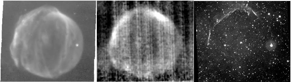
Figure 1: Left: Spitzer 24 $\mu$m image. Center: Spitzer 70 $\mu$m image. Instrument artifacts in the image introduce flux uncertainties at only the 8% level (see text for details). Right: H$\alpha$ image from 2007, courtesy of P.F. Winkler.

Tycho was observed in December of 2004 with all three instruments on Spitzer (PI J. Rho, Program ID 3483). Here, we report only on the 24 and 70 $\mu$m images from the Multiband Imaging Photometer for Spitzer (MIPS). We use the Post-Basic Calibrated Data (PBCD) from the Spitzer pipeline, version 18.12, for our analysis. We show the 24 and 70 $\mu$m images in Figure 1. The entire limb-brightened shell is seen in both images, and additional filamentary structures that run roughly in a N-S direction are visible at 24 $\mu$m. Significant variations in brightness are seen in the remnant as well, with regions in the northwest and east having surface brightnesses several times higher than elsewhere in the remnant. We discuss the flux variations further in the following sections. For further comparison, we show a high-resolution optical H$\alpha$ image (courtesy of P.F. Winkler), which shows emission only from the eastern and northern limbs.

3 Results

3.1 Measurements

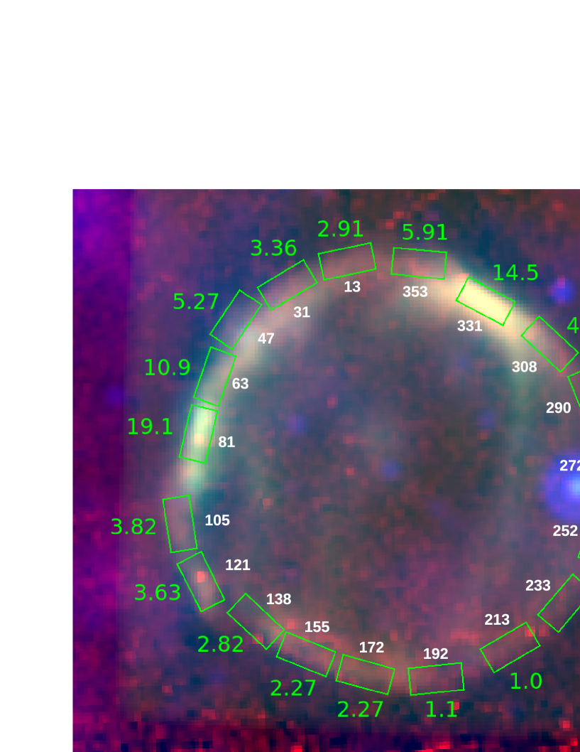
Figure 2: The normalized density in various regions of Tycho, along with outlines of the spatial regions used for our analysis, superposed on a three-color IR image, with Spitzer 70 $\mu$m emission in red, 24 $\mu$m emission in green, and WISE 12 $\mu$m in blue. North is up and east is to the left. The absolute scaling for the densities are 0.11 for the compact grain model and 0.2 for the porous grain model (see Section 4.4 and Table 2 for details). Interior numbers are azimuthal angle, in degrees.

We divided the outer shell of the remnant into equally-sized segments for our analysis, where each section is $30^{\prime\prime}$ in the radial direction and $60^{\prime\prime}$ in the tangential direction. The radial dimension is chosen to be slightly larger than the point-spread function of Spitzer at 70 $\mu$m, which is approximately $20^{\prime\prime}$, to ensure that all flux from the rim is captured within our regions. We were able to fit 19 non-overlapping regions around the periphery of the shell, ensuring that the outer boundary of each region extends slightly beyond the extent of the IR emission in the radial direction. We show all 19 regions, plotted on top of a 3-color IR mosaic, in Figure 2. This mosaic contains, for visualization purposes only, the 12 $\mu$m image from the Wide-Field Infrared Survey Explorer (WISE).

To measure the IR flux ratio, we had to first decide which IR images to use. We had six choices: 12 and 22 $\mu$m from WISE, 24 and 70 $\mu$m from Spitzer, and 70 and 100 $\mu$m from Herschel. We chose the Spitzer data. Spitzer images at 24 and 70 $\mu$m show clear emission from the entire shell of the remnant. The 70 $\mu$m image suffers from regularly spaced “striping” artifacts related to the scan direction of the telescope during mosaic observations. This is a well-known issue with the Spitzer 70 $\mu$m MIPS detector, and one that we have encountered before (Sankrit et al., 2010). In that paper, we found that despite their unsightly appearance, the stripes contribute an overall uncertainty of only 5% to the fluxes measured at 70 $\mu$m. Here, a similar analysis of the variations found in “on-stripe” and “off-stripe” flux measurements from relatively uniform regions of the remnant produced a similar result. In all the regions we tested, most of the variations were of order 5%; the largest effect we found was 8%. Thus, we did not attempt to correct for the striping pattern; rather, we simply added an additional 8% uncertainty term to all measured fluxes at 70 $\mu$m. The MIPS Instrument Handbook lists calibration uncertainties on fluxes of extended sources at 4% and 7% for the 24 and 70 $\mu$m detectors, respectively. With the additional 8% uncertainty to the 70 $\mu$m fluxes, we conservatively assume all flux ratios to have a 16% uncertainty.

Emission from dust grains at 12 $\mu$m arises from the very smallest grains that undergo temperature fluctuations and which are particularly prone to destruction through sputtering by thermal ions. The WISE 22 $\mu$m image is essentially identical to Spitzer data at 24 $\mu$m, but the spatial resolution and sensitivity of WISE are both lower than Spitzer. For this reason, we do not use either of the WISE images in our analysis.

The Herschel data present two issues. First, while the shell of the remnant is clearly detected at 70 $\mu$m, the detection at 100 $\mu$m is rather weak (see Figure 8 of Gomez et al. (2012)). Thus, our decision is between the 70 $\mu$m data from Herschel and Spitzer. Ideally, we would use the Herschel data, since the spatial resolution of Herschel is several times better than Spitzer, making the Herschel 70 $\mu$m image of comparable spatial resolution to the Spitzer 24 $\mu$m image. However, the second issue with Herschel data is calibration uncertainty. Recent work by Aniano et al. (2012) has revealed significant issues with the extended source photometry calibration of the PACS instrument on Herschel, which contains the 70 $\mu$m camera. Because we are only doing two-point photometry to constrain the temperature of dust grains, it is crucial that the two fluxes that we use are calibrated as closely to each other as possible.

With our 19 spatial regions defined, measuring the flux is straightforward. We first convolve the 24 $\mu$m image to the resolution of the 70 $\mu$m image using the convolution kernels provided in Gordon et al. (2008). We define a background that consists of four separate regions, each a few arcminutes outside of the remnant, to the NE, NW, SW, and SE of the shell. Although the background is fairly uniform in the immediate surroundings of Tycho, we average these four regions to create a single off-source background that we subtract from each flux measurement (scaled to the size of our extraction regions).

We report our flux measurements at 24 and 70 $\mu$m in Table 1. The 24 $\mu$m flux shows significant variations as a function of azimuthal angle around the periphery of the shell, being as much as 15 times higher in the NW than in the SW. The 70 $\mu$m flux varies by only a factor of two around the shell. The different behavior of the two fluxes is quite significant: the remnant is not only brighter in some places than in others, but the ratio of the 70 $\mu$m flux to the 24 $\mu$m flux, and thus the temperature of the dust, varies by nearly an order of magnitude from one place to another in the remnant. It is the ratio of the 70 to 24 $\mu$m flux that we fit with our models, described below, to determine the gas density behind the shock.

3.2 Modeling

As previously stated, the ratio of IR fluxes resulting from emission from warm dust grains is a diagnostic of the conditions of the X-ray emitting plasma. We have developed spectral models for dust emission in SNRs; we refer the reader to Williams et al. (2011a) for a more complete description. Briefly, the spectrum emitted by a dust grain immersed in a hot plasma depends on the temperature and density of both the electrons and ions. The grain is heated by collisions with particles, with proton and alpha particle collisions also slowly eroding the grain via sputtering (Nozawa et al., 2006). These grains exist in the ISM encountered by the forward shock wave of the SNR, and are not newly-formed grains from the SN ejecta. Grain properties are important as well: large grains are heated to lower temperatures than small grains. The smallest grains (below a few nm in size) emit radiation quickly enough that they cool back down to their ambient temperatures before being hit again (Draine, 2003), and these stochastic temperature fluctuations must be taken into account. Larger grains reach an equilibrium temperature determined by the balance between the collisional grain heating rate and the grain radiative cooling rate. Smaller grains are more quickly destroyed via sputtering. The optical properties of the grain are also important, e.g., the IR spectrum from a carbonaceous grain looks different from that of a silicate grain (Draine & Lee, 1984).

Our models take all of the above effects into account. We use the dust grain size distributions of Weingartner & Draine (2001), which contain a mix of carbonaceous and silicate grains ranging in size from 1 nm to 1 $\mu$m, in proportions appropriate for the ISM of the Milky Way. We use their favored model for the ISM in the Milky Way, with $R_{V}$ (the ratio of visual extinction to reddening) of $3.1$ and $b_{c}$ (a parameterization of the carbon abundance in small grains) of $6.0$, though we note that the choice of grain-size distribution does not significantly affect the derived fits to the IR emission (Williams et al., 2006). Once the grain properties are defined, what remains is to determine the plasma conditions. Because grains are heated by the forward-shocked gas of roughly cosmic abundances and we assume that the contribution of heavier elements to the gas density is small, we can assume that the post-shock electron density is 20% higher than the proton density, i.e. $n_{e}=1.2n_{p}$, while the alpha particle density is one-tenth the proton density, i.e. $n_{\alpha}=0.1n_{p}$.

3.2.1 Ion Temperature

Determining the plasma temperatures for the various regions in Tycho is not necessarily straightforward, but we use the following approach. First, for the proton temperature, we assume the standard shock jump conditions derived from the Rankine-Hugoniot conditions:

$$kT_{p}=\frac{3}{16}m_{p}v_{s}^{2},$$ (1)

where $m_{p}$ is the mass of a proton and $v_{s}$ is the shock velocity. To determine the shock velocity, we use the proper motion measurements from radio (Reynoso et al., 1997) and X-ray (Katsuda et al., 2010) studies, scaling the expansion rate to a distance of 2.3 kpc. Both of these studies report the proper motion of the forward shock as a function of azimuthal angle for the entire periphery of the remnant, and the agreement between the two is generally within 20% (although, in select locations, the discrepancy between the two measurements is as high as 40%). Because of this, we simply use an average of the radio and X-ray values to determine the shock velocities. For the regions in which the X-ray and radio proper motions agree to within 10%, we assign an uncertainty of 10% to the shock velocity, approximately equal to the errors reported in both papers. In areas where the discrepancy is greater than this, we use the absolute values of the difference between the average value and that from each study for the uncertainty. The largest uncertainty in the shock velocity obtained in this way is 20%. We list all shock velocities, with uncertainties, in Table 1, along with the proton temperatures derived from these shock velocities. We assume that the downstream energy loss of the protons to Coulomb collisions has been minimal, consistent with the low values for temperature equilibration found in the H$\alpha$-emitting shocks by Ghavamian et al. (2000). We also assume that alpha particle temperatures are four times higher than proton temperatures, i.e., that ion-ion equilibration is negligible. This is consistent with results from SN 1006, where shocks of similar speed have been found to have minimal ion-ion equilibration (Laming et al., 1996).

There are several caveats to the proton temperature determination. First, as previously mentioned, temperature equilibration will bring the proton and electron temperatures closer together. However, after a fast initial rise in the electron temperature from $\sim 10,000$ K up to a few 100,000 K, the remaining equilibration proceeds quite slowly, and is negligible in Tycho (Ghavamian et al., 2001). An additional effect is introduced by the uncertainty in the distance to Tycho. Lastly, the Rankine-Hugoniot conditions themselves assume that no energy is lost in the shock to escaping particles, an assumption which breaks down in the case of efficient cosmic-ray acceleration. Tycho may well be the site of such acceleration, as has been proposed by Warren et al. (2005) and Eriksen et al. (2011). Efficient particle acceleration will lower the post-shock proton temperature from the values we report. A factor of two change in $kT_{p}$ solely due to cosmic-ray acceleration would imply a compression ratio of $\sim 10$ (Vink et al., 2010).

However, the effects of these uncertainties in the proton temperature on the modeling of warm dust emission are not large. Even a factor of two variation in $kT_{p}$ only results in a 25% change in the inferred densities. We can quantify the dependence of the densities we report in Section 4 on the uncertainty in the distance. We assume D = 2.3 kpc, but if the distance were, for instance, 3 kpc, the proton temperatures implied by the shock velocities would be 70% higher. Higher temperatures would lead to lower densities, but the densities we report would only be lower by a factor of 1.2. Finally, it is important to note that these uncertainties in the proton temperature will affect only the absolute determinations of the density, and not the relative density from place to place in the remnant.

3.2.2 Electron Temperature

Hwang et al. (2002) report electron temperatures of around 2 keV in Tycho based on a 49 ks Chandra observation in September of 2000. Atomic databases used in X-ray modeling codes like XSpec have been updated significantly since 2002. We reanalyze the X-ray data for this paper, using NEI version 2.0, augmented by custom atomic line codes which include missing inner-shell electron transitions (Badenes et al., 2006). Since Tycho was reobserved for significantly longer in 2009, we use the new data, but repeat the analysis of Hwang et al. (2002). We also include XMM-Newton observations (PI A. Parmar) and fit both spectra independently.

We derive a slightly lower temperature of 1.35 keV. To explore the discrepancy between our fits and those from Hwang et al. (2002), we applied the spectral models used to fit the 2009 data to the original 2000 data, finding the same lower temperature. We obtain statistically identical fits from the XMM-Newton data. We believe the most likely explanation for the discrepancy between Hwang et al. (2002) and our work is simply a change in the calibration of the telescope and/or updated atomic data over the last decade. We therefore set the electron temperature at 1.35 keV, and make the assumption that this is the temperature in every region around the periphery of the shock.

Obviously, this assumption is unlikely to be correct everywhere along the rim. But how much does the value of the electron temperature matter for our dust modeling? As it turns out, it matters even less than the proton temperature does. A factor of two difference in the electron temperature has only a 10% effect on the ratio of the IR fluxes measured in the Spitzer bands. The difference between 1.35 and 2 keV, the value reported in Hwang et al. (2002), has only a 5% effect on the density. Because the efficiency of grain heating by electrons decreases with increasing electron temperature, values higher than 2 keV have virtually no added effect on lowering the densities we calculate. However, lower electron temperatures can raise the inferred densities. The lowest observed value for the electron/proton temperature ratio at a collisionless shock is $\sim 0.05$, found in SN 1006 (Vink et al., 2003). In the theoretical models of van Adelsburg et al. (2008), shocks of greater than 1500 km s^-1 have a minimum value of this ratio of 0.03. If we assume this value is the minimum possible value in Tycho, this leads to a minimum electron temperature of around 0.3 keV, which is also the minimum level of electron heating in collisionless shocks predicted by the lower hybrid wave model of Ghavamian et al. (2007). Since electron temperatures this low are typically not found in young SNRs, this temperature can be regarded as a lower limit. The density inferred from a shock with $kT_{e}=0.3$ is a factor of 1.7 higher than that inferred from a shock with our assumed value of 1.35 keV. Thus, while we recognize that the assumption of a constant value of $kT_{e}$ is probably not valid, it is unlikely that variations from this are large (given the fact that shock speeds only vary by a factor of two in the remnant), and in any case, even significant variations do not have a large effect on the modeling.

3.2.3 Density Fits

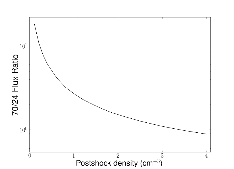
Figure 3: The 70/24 $\mu$m flux ratio as a function of gas density, assuming electron and proton temperature held constant at 1.35 and 20 keV, respectively. Note that this plot is on a logarithmic scale on the y-axis.

With the electron and proton temperatures estimated for each of the 19 regions, the density of the gas in the post-shock environment is the only remaining free parameter in our models. We adjust the density in each region to fit the measured 70/24 flux ratio. We show in Figure 3 the 70/24 flux ratio as a function of postshock density, $n_{p}$, assuming constant values of $kT_{p}$ and $kT_{e}$. The effect of the density on the flux ratio is quite large, allowing us to determine the density within a given region with relatively little uncertainty, for given values of the plasma temperature. We report the values of density in Table 2 and show them (normalized to the lowest density regions to show the magnitude of the relative density differences in the remnant) on an image of the remnant in Figure 2. Density uncertainties are calculated assuming a 16% error on the 70/24 flux ratio; see Section 1. Two inferences are immediately apparent from the inferred densities. First, there are only three regions where the density (reported as the post-shock proton density, $n_{p}$) is higher than 1 cm^-3: two contiguous regions on the eastern limb, including the “knot g” filament seen in the optical, and one region in the NW. Second, aside from these three “dense” regions, there appears to be an overall azimuthal gradient in the densities, with the average in the NE being a factor of 3-5 higher than in the SW. We discuss and interpret these results below, in Section 4.

4 Discussion

The densities we determine in the various regions around the forward shock have an inverse relationship with the shock velocities measured in these regions, as inferred from the proper motion studies. This is expected, but is not an a priori constraint of the models. It is also not simply a result of the effect of variations in the proton temperature in these regions; as we showed in Section 3.2, the effect of the proton temperature on the calculated IR flux ratio is fairly small, and certainly not enough to account for the variations seen in the density. Morphologically, the regions where the highest densities are measured are also the places where H$\alpha$ emission is seen. Our models are not directly sensitive to the pre-shock ambient density, only to that in the post-shock environment. A standard strong shock will produce a compression ratio of four between the pre and post-shock gas, but this should be considered a lower limit. Efficient particle acceleration will raise the compression ratio at the shock (Jones & Ellison, 1991).

Along the eastern and northwestern portions of the remnant, the forward shock is encountering localized denser clumps of material. In particular, the highest density region we find in the remnant corresponds to “knot g” (Kamper & van den Bergh, 1978), the brightest optical filament in the remnant. Our results in these few dense knots are qualitatively consistent with the conclusions of Ghavamian et al. (2000) that the shock in the regions of bright H$\alpha$ emission is encountering denser material from a neighboring HI cloud.

However, strong H$\alpha$ emission in Figure 1 is not confined just to a few dense knots located at the remnant’s rim, but extends over the whole NE quadrant. The longest contiguous set of filaments in the NE is located interior to the outermost blast wave. Densities along these filaments are likely significantly higher than along the remnant’s rim. Because of the poorly known shock geometry in this region of the remnant, it is not clear how the outermost blast wave related to these optical filaments. In one scenario, it might mark where the blast wave wraps around a low-density periphery of a large cloud with a high density, similar to the dense knots discussed above. Alternatively, densities along these long optical filaments might be lower, so they would fit better into the framework of the overall density gradient discussed below. In this case, the magnitude of the overall density gradient would be underestimated with the current density measurements available just at the remnant’s rim. Proper motion measurements of optical filaments are needed to resolve these ambiguities.

4.1 Density Gradient

The densities we determine clearly favor a low average ISM density, consistent with the lack of thermal X-ray emission from the blast wave. Densities in the E and NE are 3-5 times higher than those in the W and SW. As we will show below, hydrodynamical simulations are broadly consistent with this, though they suggest that the magnitude of the gradient may need to be somewhat higher, at around an order of magnitude. The simplest explanation for this behavior is a NE-SW density gradient in the ISM. This is consistent with the hypothesis of Lee et al. (2004) that Tycho is expanding into an ISM density gradient. It is also qualitatively consistent with studies of the X-ray emitting ejecta by Badenes et al. (2006) and Hayato et al. (2010), who found that the ejecta are brighter in the E and NW than in the SW. Even if our models for dust emission have systematic errors, the fact remains that the temperature of the dust, as measured by differences in the IR flux ratios, varies significantly in different locations in the remnant, and variations in the post-shock gas density are the most plausible way to explain this. It is unlikely that our models are more correct on one side of the remnant than the other. Detailed multi-dimensional modeling of the remnant’s evolution and the ionization state of the reverse-shocked ejecta is beyond the scope of this paper, but a full understanding of Tycho will require such work.

A possible alternative explanation for the apparent density gradient is cosmic-ray acceleration that is much more efficient on one side of the remnant than the other. Our dust models are insensitive to this, but to explain the density differences we see purely by an increase in the compression ratio due to particle acceleration, the shock compression ratio in the E and NE would have to be $\geq 15$. While this is not beyond the realm of possibility, it does imply that $>80$% of the total shock energy is being put into cosmic rays (Vink et al., 2010). Also, if this were the case, then the ratio of the radius of the contact discontinuity (CD) to the forward shock (FS) would be much higher in regions of such extreme compression ratios. Warren et al. (2005) examined this ratio (CD/FS) around the periphery of Tycho, finding evidence for particle acceleration everywhere in the remnant (although Orlando et al. (2012) have suggested that the high values of this ratio can be explained via hydrodynamic instabilities, without need of cosmic-ray acceleration). Furthermore, if such acceleration were taking place in regions of high density, we would expect to see a correlation between the densities we measure and the value of CD/FS from Warren et al. (2005), yet we see no such correlation in our data. Even when we throw out the three highest values of density, those apparently coming from dense knots, we still find virtually no correlation between density and CD/FS (R² = 0.14).

4.1.1 Gamma-Ray Emission

Morlino & Caprioli (2012) model the $\gamma$-ray emission from Tycho by assuming a uniform pre-shock density of 0.3 cm^-3, finding that such a medium supports a model in which the GeV and TeV emission is produced by the hadronic mechanism, i.e., protons accelerated at the blast wave colliding with ambient protons to produce $\pi^{0}$ particles, which then decay into $\gamma$-rays. However, Atoyan & Dermer (2012) find that a leptonic model of $\gamma$-rays produced via inverse-Compton scattering of energetic electrons off of low-energy photons fits the $\gamma$-ray data equally well. Their model assumes a density of 0.75 cm^-3, although they note that lower densities cannot be excluded. Only three of the nineteen regions we model can have a pre-shock density as high as the assumed density in either the hadronic or the leptonic models. Clearly, further study of the $\gamma$-ray emission from Tycho is necessary, taking into account the density structure we find here.

Interestingly, Acciari et al. (2011) reported a small offset in the TeV emission from the center of the remnant, in the direction of enhanced density to the NE. The TeV source is offset by $2.4^{\prime}$ with a statistical uncertainty of $1.4^{\prime}$, while the VERITAS telescope has a 1$\sigma$ PSF of $6^{\prime}$. However, even confirmation that the $\gamma$-ray morphology correlates with the density enhancements does not definitively select one model of $\gamma$-ray emission, as both leptonic and hadronic models could explain such a morphology. $\gamma$-ray emission from bremsstrahlung and $\pi^{0}$-decay is enhanced by the higher target density, while inverse Compton scattering off low-energy IR or microwave photons will also be enhanced in this region. We will fully examine the implications of our density finding for the $\gamma$-ray emission observed in a future publication.

4.2 An Off-Center Explosion Site

An additional effect of an explosion into a non-uniform ISM is that the center of explosion will not be at the center of the resulting remnant (Dohm-Palmer & Jones, 1996). A recent analysis by Kerzendorf et al. (2012) of six stars identified by Ruiz-Lapuente et al. (2004) within the center of Tycho did not turn up any potential candidates for the companion star, thought to exist in the single-degenerate scenario of a Type Ia SN, leading the authors to conclude that Tycho could not be explained by such a scenario. However, these authors searched for potential companion stars only within a circle of radius 39^′′ centered on the center of symmetry of the Chandra image. We report here the effects of the density gradient that we observe on the current location of the center of explosion with respect to the center of symmetry of the remnant. We have performed two-dimensional (2D) hydrodynamic modeling of Type Ia SN explosions with an exponential ejecta profile (Dwarkadas & Chevalier, 1998) into a density gradient, and have compared these results with analytic solutions to the thin-shell approximation (Carlton et al., 2011). We report both below. We find that the most model-independent way to infer the offset is from the observed velocity asymmetry, i.e., the proper motion of the shock. We assume that the observed density gradient is in the plane of the sky.

4.2.1 Hydrodynamic Modeling

For our hydrodynamic modeling, we employed the same numerical methods as described in Warren & Blondin (2013), with the additional feature of a density gradient in the ambient medium. The external density gradient was of the form $\rho\propto e^{ar}$, where $r$ is a dimensionless distance, the same as $r^{\prime}$ in Equation (3), and $1/a=r_{ISM}$ is the dimensionless ISM density scale, discussed further in the Appendix.

Specifically, we used the VH-1 hydrodynamics code to evolve the Euler equations for an ideal gas with a ratio of specific heats of $\gamma=5/3$ on a 2D spherical-polar grid with 300 radial zones by 900 angular zones, providing a spatial resolution of $\Delta\theta\approx 3.5\times 10^{-3}$ in the angular direction and slightly higher resolution in the radial direction. The supernova ejecta were modeled using the exponential density profile of Dwarkadas & Chevalier (1998). We employed a moving grid to track the evolving SNR as it expanded over five orders of magnitude, effectively removing any artifact of the initial conditions and providing sufficient time for the Rayleigh-Taylor instability of the contact interface between shocked ejecta and shocked ISM to reach a quasi-steady state.

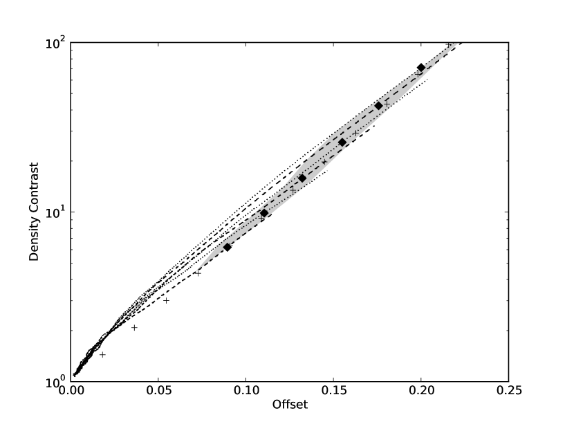
Figure 4: Offset of the explosion from the geometric center of the remnant ($R_{max}-R_{min}$)/($R_{max}+R_{min}$) versus density contrast in the ISM from one side of the remnant to the other. From top to bottom: tracks from 2D hydrodynamical simulations with values of the density gradient parameter, “$a$,” of 1.8, 1.6, 1.4, 1.2, 1.0, and 0.8. Diamonds show locations along each track of a dimensionless time of unity. The shaded gray region corresponds to dimensionless time between 0.7 and 1.3; Tycho should be located in this region. Plus signs mark analytic results for dimensionless time of unity, for values of “$a$” from 0.2 (lower-left) to 2.4 (upper-right).

We examined various values of $a$ to study the effects of the density gradient on asymmetries in the shock velocities and on the remnant shape. The values of $a$ correspond to a range of current density contrasts at the current size of Tycho of factors of 5-100 from maximum to minimum. An important result of our simulations is that the ratio of the velocity semi-amplitude ((V_max - V_min)/(V_max + V_min)) to the radial offset from the center of the explosion ((R_max - R_min)/(R_max + R_min)) is roughly constant at a value of about 2.2 $\pm$ 0.1 for ages between about 300 and 700 yr. Our simulations predict, for different values of $a$ and different ages, relations between the radial offset and the density gradient. These relations are summarized in Figure 4, which shows that for a wide range of gradients and ages, there is a fairly tight relation between the density contrast across the remnant and the radial offset. One can then use either an observed density contrast or shock proper motions to predict the radial offset of the explosion site from the symmetry center for a remnant.

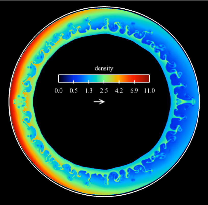
Figure 5: Simulated remnant from a 2D hydrodynamical simulation at an age of several hundred years, expanding into an exponential density gradient with $a=0.95$. At the time shown, the upstream density is an order of magnitude higher on the left than the right. The density scale is in dimensionless units, and only the shocked gas is shown. The offset of the center of the explosion from the current center of symmetry of the blast wave is shown with an arrow, and amounts to roughly 10%. The outer white circle is perfectly round, and is simply shown for comparison to illustrate the roundness of the simulation.

For Tycho, Table 1 shows that the velocity semi-amplitude of the averaged velocities from the radio and X-ray measurements is 0.36 (the velocities reported in that Table assume D=2.3 kpc, but since the velocity semi-amplitude is dimensionless, it is also independent of distance). Dividing this by the ratio of 2.2, given above, we obtain a radial offset of 16.5% of the radius of the remnant, or about $40^{\prime\prime}$ from the geometric center of the remnant to the explosion site. The discrepancies between the radio and X-ray measurements are relevant here. Using the X-ray data alone, the velocity semi-amplitude is only 0.22, which leads to an offset of $25^{\prime\prime}$, within the search radius of Kerzendorf et al. (2012). Using the radio data alone, we obtain a velocity semi-amplitude of 0.51, leading to an offset of $1^{\prime}$. Figure 5 shows our simulated remnant at an age roughly corresponding to that of Tycho, and assuming a value of $a$ of 0.95, giving a current density contrast of about an order of magnitude. This demonstrates that the remnant (in the relatively early evolutionary stage of Tycho) can remain remarkably round despite a significant external density gradient. A qualitatively similar result, for a considerably different functional form of density gradient, was obtained by Dohm-Palmer & Jones (1996).

The large offset inferred from the radio proper motions alone can likely be ruled out by the results of our hydrodynamic and analytical modeling shown in Figure 4. An offset of 1^′ would require a density contrast of approximately 80, well above what we measure from the IR data. Clearly, better proper motion measurements are necessary to resolve this discrepancy. We have recently been approved for new JVLA observations, which will expand the baseline for proper motion measurements from the 11 years reported in Reynoso et al. (1997) to $\sim 30$ years, significantly reducing the uncertainties on the proper motions. Nonetheless, we suggest that searches for the progenitor companion in Tycho be extended by a factor of two beyond the area searched by Kerzendorf et al. (2012).

4.2.2 Analytic Approximation

Carlton et al. (2011) present a thin-shell approximation to a blast wave expanding into a uniform ISM, and here we extend their results to an ambient density gradient. There are analytic solutions in the thin-shell approximation for both linear and exponential density gradients (see the Appendix). For the linear gradient, we derive an approximate expression for the ratio of the dimensionless velocity semi-amplitude to the radial offset. A full derivation is presented in the Appendix, but the key results here are 1) the ratio from the analytic approximation is 2.4, quite close to the 2.2 determined from the hydrodynamic simulations above; and 2) this approximate expression holds even for large density contrasts inferred for Tycho where use of the exponential (instead of linear) density gradient is preferred.

4.3 Pressure

With the density and velocity known, we can calculate the ram pressure in the shock, $\rho_{0}v_{s}^{2}$. We divide the post-shock number densities by four to convert to pre-shock densities, then multiply that by [1.4 $\times$ (1.67 $\times 10^{-24}$)] g to get a mass density, $\rho_{0}$. We report the ram pressure for each region in Table 2. In the east and NW knots, the pressures are a factor of 5-10 higher than elsewhere in the remnant, supporting the idea of a relatively recent encounter with denser clumps, where the pressure has not yet had time to equilibrate. Elsewhere in the remnant, pressures in the SW are about a factor of two lower than those in the NE, in good agreement with our hydrodynamic modeling. The same caveat applies here about particle acceleration increasing the compression ratio of the gas. If the compression ratio were higher in the NW, then the ram pressures of the shock could be more equal. If particle acceleration is constant in the remnant, only the absolute values of the pressure will be affected, but the relative differences will remain.

4.4 Evolutionary State of Tycho

The densities we report in Table 2 assume a distance to Tycho of 2.3 kpc and “standard” ISM dust grains, i.e., compact, homogeneous spheres with a mix of silicate and graphite grains in separate populations. If we ignore the three regions coincident with dense knots, the azimuthally-averaged value of the post-shock density is $\sim 0.3$ cm^-3. Under the assumption of standard shock jump conditions, this leads to an average pre-shock density, n₀, of around 0.08-0.1 cm^-3. Since the IR emission is produced throughout the post-shock region where densities decrease from their value right behind the blast wave, the density ratio averaged over that region is expected to be somewhat less than 4 (Williams et al., 2011a). This density, while below the upper limit of 0.2-0.3 cm^-3 reported by Cassam-Chenaï et al. (2007) & Katsuda et al. (2010), is rather low, given what is known about the evolutionary state of Tycho.

To first-order, the average density obtained for a density gradient is equal to the density being encountered by the forward shock in a direction perpendicular to the gradient. For Tycho, this would correspond to position angles of $\sim 140$ and $320^{\circ}$. Following the scaling of hydrodynamical variables by Dwarkadas & Chevalier (1998), we can write the dimensionless scaled radius, $r^{\prime}\equiv r/R^{\prime}$, and the scaled time $t^{\prime}\equiv t/T^{\prime}$ as

$$r^{\prime}=0.61\ (n_{0}/0.1\ {\rm cm}^{-3})^{1/3}\ (D/2.3\ {\rm kpc})\ (M_{ej}/M_{Ch})^{-1/3},$$ (2)

$$t^{\prime}=0.82\ (n_{0}/0.1\ {\rm cm}^{-3})^{1/3}\ E_{51}^{1/2}\ (M_{ej}/M_{Ch})^{-5/6},$$ (3)

where M_ej is the ejecta mass, M_Ch is the Chandrasekhar mass, and $E_{51}$ is the explosion energy in units of $10^{51}$ ergs. Assuming a standard Type Ia explosion where M_ej = M_Ch, a pre-shock density of 0.08 leads to a scaled radius of 0.57. Comparing this with the three-dimensional hydrodynamic simulations of Warren & Blondin (2013), a scaled radius of 0.57 for the forward shock implies a scaled time (again, using the formalism of Dwarkadas & Chevalier 1998) of only $\sim 0.4$. This is too short to explain the expansion parameter, $m$ (where r $\propto$ t^m), of Tycho, known from proper motion measurements to be $\sim 0.53$ (Reynoso et al., 1997; Katsuda et al., 2010). Recent three-dimensional hydrodynamical simulations of Warren & Blondin (2013) show that this can be achieved with a scaled time of around 1, corresponding to a scaled radius also around 1-1.1. Our hydro simulations confirm this; the expansion parameter and velocity semi-amplitude in Tycho are best matched in simulations with a scaled time of 1.05 and a scaled radius of 1.15.

Thus, our scaled radius needs to be increased by about 70% to match hydrodynamic simulations of the evolutionary state of Tycho. There are three parameters in equation (2): $n_{0}$, $D$, and $M_{ej}$. A sub-Chandrasekhar ejecta mass would raise $r^{\prime}$, but only as M${}_{ej}^{-1/3}$, so we view this as the least viable option. If distance alone were varied, a distance of 3.9 kpc would suffice. This would lower the density slightly (see Section 3.2), but since the effect on density would be small and $r^{\prime}$ only goes as n${}_{0}^{1/3}$, the overall effect of the lowered density on $r^{\prime}$ would be trivial. A distance of 3.9 kpc is at the high end of the range of reported distances for Tycho (see Section 1), and it is worth noting that such a distance combined with measured proper motions would imply that shock velocities exceed 6000 km s^-1 in some locations.

A third, perhaps most intriguing possibility, is that the densities may be higher than we report in Table 2 due to alternative grain models. The assumption that dust grains are compact, spherical, solid bodies of homogeneous material makes for easier calculations, but is unlikely to be a physically valid model (Shen et al., 2008). In Williams et al. (2011a), we explored the effect of porosity, or “fluffiness,” as well as that of a non-homogeneous grain material, on the IR spectra produced from collisionally-heated grains. The details of our grain model are discussed in that paper; we use an identical model here. For grains that are 50% vacuum, 33.5% silicate and 16.5% amorphous carbon, the densities we infer from the IR flux ratios are increased by $\sim 80\%$. This increase in the density would raise the scaled radius to 0.7. While this is not, by itself, enough to account for the observed evolutionary state of Tycho, it can be combined with a more modest distance increase to only 3.3 kpc. The resulting average density from this model would be 0.14-0.15, which is still below the upper limits of 0.2-0.3 discussed earlier. While this is suggestive that porous grains may, in fact, be ubiquitous in the ISM, current knowledge of grain physics is insufficient to conclusively rule on this issue. Grains of even higher porosity would have a larger effect on raising the density, and grains exceeding 90% porosity have been suggested to fit the IR spectra of some stars (Li & Greenberg, 1998). Finally, we point out that while the choice of grain model can affect the absolute density values one determines, the relative values are unchanged, and the inference of a density gradient in Tycho is unaffected.

5 Conclusions

Observations of Tycho in the mid-IR reveal significant color variations in the forward shock-heated interstellar dust. Since this dust is warmed by collisions with energetic particles in the postshock gas, the IR observations are a powerful diagnostic of the gas density in the remnant. We analyzed IR emission as a function of azimuthal angle around the periphery of the forward shock, finding a variation in the ratio of the 70 $\mu$m to 24 $\mu$m flux of an order of magnitude, implying an overall density gradient with densities higher in the NE than in the SW by a factor of $\sim 3-5$. This ISM density gradient is virtually independent of distance and assumed dust grain composition. We also identify a few regions of significantly higher density that morphologically correspond to bright H$\alpha$ emitting regions. These are likely localized density enhancements produced during the early stages of interaction with a nearby HI cloud.

Tycho joins the growing group of Type Ia SNRs that are not consistent with expansion into a uniform ISM. We use two-dimensional hydrodynamic simulations of Type Ia SN explosions into a density gradient and find that the explosion center of the remnant must be shifted with respect to the geometric center of the remnant by around 10%, and possibly higher. In Tycho, these computational simulations agree quite well with analytic approximations. The simulations suggest that the magnitude of the density gradient may need to be even higher than inferred from IR observations, around a factor of 5-10, to explain the proper motions observed in the remnant. The offset of the explosion in the simulations is most sensitive to the observed proper motion variations of the forward shock, so improved proper motion measurements of Tycho are necessary for further study. Finally, simulations show that remnants expanding into a significant density gradient can remain remarkably round.

The mean upstream densities in Tycho are relatively low ($\sim 0.1-0.2$ cm^-3, depending on the assumed dust model), consistent with the lack of thermal X-ray emission from most places along the forward shock in Tycho (with the exception of the NW). The densities inferred from models of standard ISM dust grains are too low to explain the evolutionary state of Tycho. Porous grains provide a potential resolution to this, as inferred densities from such grain models are significantly higher. A distance of around 3.5 kpc would also resolve this issue. Our results suggest that Tycho is far from a spherically symmetric, homogenous remnant, and multi-dimensional modeling is required for a fuller understanding.

Facilities: Chandra, Spitzer, XMM-Newton

Table 1: Measurements

Deg.	24 $\mu$m Flux	70 $\mu$m Flux	70/24 Flux Ratio	$V_{s}$ (km s-1)	TP (keV)
13	201	1319	6.96 $\pm 1.1$	3660 $\pm 366$	26.0
31	223	1373	5.97 $\pm 0.93$	3310 $\pm 331$	21.3
47	226	1358	5.42 $\pm 0.84$	2360 $\pm 236$	10.9
63	514	1592	3.50 $\pm 0.54$	1920 $\pm 378$	7.1
81	1093	1739	2.09 $\pm 0.32$	2210 $\pm 378$	9.5
105	279	1394	6.07 $\pm 0.94$	3110 $\pm 311$	18.8
121	315	1441	5.99 $\pm 0.93$	3510 $\pm 351$	24.0
138	198	1319	7.65 $\pm 1.2$	3330 $\pm 333$	21.6
155	181	1361	8.79 $\pm 1.4$	3480 $\pm 538$	23.6
172	184	1369	9.21 $\pm 1.4$	3240 $\pm 486$	20.4
192	103	1281	15.10 $\pm 2.3$	3780 $\pm 378$	27.8
213	99	1304	15.70 $\pm 2.4$	4060 $\pm 634$	32.1
233	94	1339	15.92 $\pm 2.5$	3980 $\pm 418$	30.9
252	88	1211	14.33 $\pm 2.2$	3920 $\pm 648$	29.8
272	96	1248	13.70 $\pm 2.1$	3850 $\pm 385$	28.8
290	110	1168	10.58 $\pm 1.6$	3700 $\pm 370$	26.6
308	346	1499	4.34 $\pm 0.67$	3580 $\pm 358$	24.9
331	1362	2113	1.98 $\pm 0.31$	3200 $\pm 320$	19.9
353	273	1426	5.02 $\pm 0.78$	2380 $\pm 238$	11.0

Note. — Deg. = Azimuthal angle, east of north. All fluxes reported in milliJanskys. Errors on fluxes are 4% for 24 $\mu$m and 15% for 70 $\mu$m (see Section 1 for details). $V_{s}$ = shock velocity, averaged from radio and X-ray measurements and assuming D=2.3 kpc. T_P = proton temperature.

Table 2: Results

Deg.	Density (cm-3)	Pressure (dyne cm-2)
13	0.32${}^{0.40}_{0.27}$	2.51${}^{3.16}_{2.01}$ $\times 10^{-8}$
32	0.37${}^{0.46}_{0.31}$	2.37${}^{2.99}_{1.90}$ $\times 10^{-8}$
47	0.58${}^{0.72}_{0.48}$	1.89${}^{2.38}_{1.52}$ $\times 10^{-8}$
63	1.2${}^{1.5}_{1.0}$	2.59${}^{3.39}_{1.92}$ $\times 10^{-8}$
81	2.1${}^{2.6}_{1.7}$	6.00${}^{7.77}_{4.55}$ $\times 10^{-8}$
105	0.42${}^{0.52}_{0.35}$	2.37${}^{2.99}_{1.90}$ $\times 10^{-8}$
121	0.4${}^{0.50}_{0.33}$	2.88${}^{3.62}_{2.31}$ $\times 10^{-8}$
138	0.31${}^{0.38}_{0.26}$	2.00${}^{2.52}_{1.61}$ $\times 10^{-8}$
155	0.25${}^{0.31}_{0.21}$	1.77${}^{2.28}_{1.36}$ $\times 10^{-8}$
172	0.25${}^{0.31}_{0.21}$	1.53${}^{1.97}_{1.18}$ $\times 10^{-8}$
192	0.12${}^{0.15}_{0.10}$	1.00${}^{1.26}_{0.80}$ $\times 10^{-8}$
213	0.11${}^{0.14}_{0.09}$	1.06${}^{1.36}_{0.81}$ $\times 10^{-8}$
233	0.11${}^{0.14}_{0.09}$	1.02${}^{1.29}_{0.82}$ $\times 10^{-8}$
252	0.12${}^{0.15}_{0.10}$	1.08${}^{1.39}_{0.82}$ $\times 10^{-8}$
272	0.13${}^{0.16}_{0.11}$	1.13${}^{1.42}_{0.91}$ $\times 10^{-8}$
290	0.19${}^{0.24}_{0.16}$	1.52${}^{1.92}_{1.22}$ $\times 10^{-8}$
308	0.54${}^{0.67}_{0.45}$	4.05${}^{5.10}_{3.25}$ $\times 10^{-8}$
331	1.6${}^{2.0}_{1.3}$	9.58${}^{12.1}_{7.69}$ $\times 10^{-8}$
353	0.65${}^{0.81}_{0.54}$	2.15${}^{2.71}_{1.73}$ $\times 10^{-8}$

Note. — Densities are postshock. Pressure calculation assumes compression ratio of 4 at the shock front. Both assume standard ISM dust grain models of Weingartner & Draine (2001) and D=2.3 kpc (see text for details of dependence on these quantities).

Appendix A Thin-Shell Solution

For young Type Ia SNRs, 3-D hydrodynamical simulations by Warren & Blondin (2013) showed that the average radius of the contact interface between the shocked ejecta and the shocked ambient medium depends only weakly on details of the postshock flow. It then becomes possible to use a thin-shell approximation to follow expansion of the remnant. In this approximation, shocked ejecta and shocked ambient medium are assumed to reside in an infinitely-thin shell located at radius $R_{s}$ at time $t$ after the explosion and moving with velocity $V_{s}$. The velocity $v$ of the freely-expanding ejecta at the reverse shock is equal to $R_{s}/t$. In the exponential ejecta model of Dwarkadas & Chevalier (1998), the shocked ejecta mass $M_{ej}$ is equal to

$$\frac{M_{ej}}{M_{ej}^{tot}}=\frac{1}{2}\left[\left(\frac{v}{v_{e}}\right)^{2}+2\frac{v}{v_{e}}+2\right]\exp\left(-\frac{v}{v_{e}}\right),$$ (A1)

where $M_{ej}^{tot}$ is the total ejecta mass and $v_{e}$ is the exponential velocity scale ($\rho_{ej}\propto\exp(-v/v_{e})$). The shell momentum $P_{s}$ is equal to the momentum of the shocked ejecta

$$\frac{P_{s}}{vM_{ej}}=\frac{\left(v/v_{e}\right)^{2}}{\left(v/v_{e}\right)^{2}+2v/v_{e}+2}+\frac{3v_{e}}{v},$$ (A2)

since the ambient ISM is assumed to be at rest. The shell velocity $V_{s}$ is equal to the shell momentum divided by the total shell mass, $P_{s}/(M_{ej}+M_{ISM})$ ($M_{ISM}$ is the shocked ISM mass). Equation of motion for the shell is $dR_{s}/dt=V_{s}$, which can be transformed to

$$\frac{v}{R_{s}}\frac{dR_{s}}{dv}=\left(1-\frac{vM_{ej}\left(1+M_{ISM}/M_{ej}\right)}{P_{s}}\right)^{-1}$$ (A3)

by changing the independent variable from $t$ to $v$. For uniform ISM ($M_{ISM}\propto R^{3}$), Carlton et al. (2011) reported an exact solution to equations (A1–A3):

$$r_{0}=\left[1+4\frac{v_{e}}{v}+6\left(\frac{v_{e}}{v}\right)^{2}\right]^{1/3}\left(\frac{2v}{v_{e}}\right)^{1/3}\exp\left(-\frac{v}{3v_{e}}\right),$$ (A4)

where the dimensionless radius $r_{0}$ is now normalized to unity for the swept-up ISM mass equal to $M_{ej}^{tot}$, as in Dwarkadas & Chevalier (1998). The dimensionless time is equal to $r_{0}\left(v/3^{1/2}2v_{e}\right)^{-1}$ (also in Dwarkadas & Chevalier (1998) units).

Equations (A1–A3) can be solved analytically for more complex ISM density distributions than simple power laws in $R$ discussed by Carlton et al. (2011). We consider here an exponential density distribution $\rho_{ISM}\propto\exp(ar)$, where $1/a=r_{ISM}$ is the dimensionless ISM density scale, negative (positive) for density decreasing (increasing) with radius. For $|ar|<<1$, the exponential density profile becomes linear, so solutions discussed below encompass both linear and exponential profiles. The swept-up mass is

$$m_{ISM}=3r^{3}\left[\left(\frac{1}{ar}-\frac{2}{\left(ar\right)^{2}}+\frac{2}{\left(ar\right)^{3}}\right)e^{ar}-\frac{2}{\left(ar\right)^{3}}\right]$$ (A5)

in dimensionless units. By changing variables from $v$ and $R$ to $y=(ar_{0})^{3}$ and $x=ar$ in equations (A1–A3), we arrive at

$$x\frac{dy}{dx}=4a^{3}m_{ISM}-y=12\left[\left(x^{2}-2x+2\right)e^{x}-2\right]-y.$$ (A6)

A solution

$$y=\frac{12}{x}\left[\left(x^{2}-4x+6\right)e^{x}-6-2x\right]$$ (A7)

relates the scaled shell radius $x=ar$ to the scaled swept-up ISM mass $y=(ar_{0})^{3}$ for ejecta entering the reverse shock with the same free-expansion velocity $v$ for both exponentially- and uniformly-distributed ambient medium. Expansion in Taylor series at $x=0$ gives

$$y=x^{3}+\frac{3x^{4}}{5}+\frac{x^{5}}{5}+\ldots,$$ (A8)

where the first two terms on the right-hand side provide an exact solution for the linear density gradient.

Displacement $\delta r$ between solutions (A7) and (A4), evaluated at the same time $t$ but with different ejecta velocities $v$ and $v_{0}$, respectively, is given by equations

$$\frac{\delta r}{r_{0}}=\frac{r(v)-r_{0}(v_{0})}{r_{0}(v_{0})}=\frac{v_{0}-v}{v}, v_{0}r(v)=vr_{0}(v_{0}).$$ (A9)

Generally, there is no simple explicit solution for $v_{0}$ and $\delta r$, but for small displacements a Taylor series expansion gives

$$\frac{\delta r}{r_{0}}=-\frac{3z\left(1+4z+6z^{2}\right)a}{5\left[1+6z\left(1+3z+4z^{2}\right)\right]},$$ (A10)

where $z\equiv v_{e}/v_{0}$. The dimensionless offset $(R_{max}-R_{min})/(R_{max}+R_{min})$ between the center of the remnant and the true explosion center is then equal to $|\delta r/r_{0}|$. The dimensionless velocity semiamplitude $(V_{max}-V_{min})/(V_{max}+V_{min})$ is also linear in $a$, so their ratio

$$\frac{\left(V_{max}-V_{min}\right)/\left(V_{max}+V_{min}\right)}{\left(R_{max}-R_{min}\right)/\left(R_{max}+R_{min}\right)}=2+\frac{3z\left(1+8z+24z^{2}+24z^{3}+12z^{4}\right)}{\left[1+6z\left(1+3z+4z^{2}\right)\right]\left[1+3z\left(1+2z+2z^{2}\right)\right]}$$ (A11)

is independent of the magnitude of the density gradient. For young SNRs such as Tycho, the second term on the right-hand side of this equation varies only slowly with $z$, so at the age of Tycho the ratio between the dimensionless velocity semiamplitude and the dimensionless offset may be considered independent of age and equal to 2.4.

References

- Acciari et al. (2011) Acciari, V.A., et al. 2011, ApJ, 730, 20
- Albinson et al. (1986) Albinson, J.S., Tuffs, R.J., Swinbank, E., & Gull, S.F. 1986, MNRAS, 219, 427
- Aniano et al. (2012) Aniano, G. 2012, ApJ, 756, 138
- Atoyan & Dermer (2012) Atoyan, A. & Dermer, C.D. 2012, ApJ, 749, 26
- Baade (1945) Baade, W., ApJ, 102, 309
- Badenes et al. (2006) Badenes, C., Borkowski, K.J., Hughes, J.P., Hwang, U., & Bravo, E. 2006, ApJ, 645, 1373
- Blair et al. (2007) Blair, W.P., Ghavamian, P., Long, K.S., Williams, B.J., Borkowski, K.J., Reynolds, S.P., & Sankrit, R. 2007, ApJ, 662, 998
- Carlton et al. (2011) Carlton, A., Borkowski, K.J., Reynolds, S.P., Hwang, U., Petre, R., Green, D.A., Krishnamurthy, K., & Willett, R. 2011, ApJ, 737, 22
- Cassam-Chenaï et al. (2007) Cassam-Chenaï, G., Hughes, J.P., Ballet, J., & Decourchelle, A. 2007, ApJ, 665, 315
- Chevalier et al. (1980) Chevalier, R.A., Kirshner, R.P., & Raymond, J.C. 1980, ApJ, 235, 186
- Dickel et al. (1982) Dickel, J.R., Murray, S.S., Morris, J., Wells, D.C. 1982, ApJ, 257, 145
- Dohm-Palmer & Jones (1996) Dohm-Palmer, R.C., & Jones, T.W. 1996, ApJ, 471, 279
- Draine & Lee (1984) Draine, B.T. & Lee, H.M. 1984, ApJ, 285, 89
- Draine (2003) Draine, B.T. 2003, ARA&A, 41, 241
- Dwarkadas & Chevalier (1998) Dwarkadas, V.V., & Chevalier, R.A. 1998, ApJ, 497, 807
- Dwarkadas (2000) Dwarkadas, V.V. 2000, ApJ, 541, 418
- Dwek (1987) Dwek, E., 1987, ApJ, 322, 812
- Dwek et al. (1996) Dwek, E., Foster, S.M., & Vancura, O. 1996, ApJ, 457, 244
- Eriksen et al. (2011) Eriksen, K.E., et al. 2011, ApJ, 728, 28
- Foster et al. (2012) Foster, A.R., Ji, L., Smith, R.K., & Brickhouse, N.S. 2012, ApJ, 756, 128
- Ghavamian et al. (2000) Ghavamian, P., Raymond, J.C., Hartigan, P., & Blair, W.P. 2000, ApJ, 535, 266
- Ghavamian et al. (2001) Ghavamian, P., Raymond, J.C., Smith, R.C., & Hartigan, P. 2001, ApJ, 547, 995
- Ghavamian et al. (2007) Ghavamian, P., Laming, J.M., & Rakowski, C.E. 2007, ApJ, 654, 69
- Giordano et al. (2012) Giordano, F., et al. 2012, ApJ, 744, 2
- Gomez et al. (2012) Gomez, H.L., et al. 2012, MNRAS, 420, 3557
- Gordon et al. (2008) Gordon, K.D., Engelbracht, C.W., Rieke, G.H., Misselt, K.A., Smith, J.-D. T., & Kennicutt, R.C. 2008, ApJ, 682, 336
- Hayato et al. (2010) Hayato, A., et al. 2010, ApJ, 725, 894
- Hines et al. (2004) Hines, D.C., et al. 2004, ApJS, 154, 290
- Hughes (2000) Hughes, J.P. 2000, ApJ, 545, 53
- Hwang et al. (2002) Hwang, U., Decourchelle, A., Holt, S., & Petre, R. 2002, ApJ, 581, 1101
- Ishihara et al. (2010) Ishihara, D., Kaneda, H., Furuzawa, A., Suzuki, T., Koo, B.-C., Lee, H.-G., Lee, J.-J., & Onaka, T. 2010, A&A, 521, 61
- Jones & Ellison (1991) Jones, F.C. & Ellison, D.C. 1991, Space Sci. Rev., 58, 259
- Kamper & van den Bergh (1978) Kamper, K.W. & van den Bergh, S. 1978, ApJ, 224, 851
- Katsuda et al. (2010) Katsuda, S., Petre, R., Hughes, J.P., Hwang, U., Yamaguchi, H., Hayato, A., Mori, K., Tsunemi, H. 2010, ApJ, 709, 1387
- Kerzendorf et al. (2012) Kerzendorf, W.E. et al., 2012, arXiv:1210:2713
- Kirshner et al. (1987) Kirshner, R., Winkler, P.F., & Chevalier, R.A. 1987, ApJ, 315, 135
- Krause et al. (2008) Krause, O., Tanaka, M., Usuda, T., Hattori, T., Goto, M., Birkmann, S., & Nomoto, K. 2008, Nature, 456, 617
- Laming et al. (1996) Laming, J.M., Raymond, J.C., McLaughlin, B.M., & Blair, W.P. 1996, ApJ, 472, 267
- Lee et al. (2004) Lee, J.-J., Koo, B.-C., & Tatematsu, K. 2004, ApJ, 605, 113
- Li & Greenberg (1998) Li, A. & Greenberg, J.M. 1998, A&A, 331, 291
- Moffett et al. (2004) Moffett, D., Caldwell, C., Reynoso, E., & Hughes, J. 2004, in Young Neturon Stars and their Environments, IAU Symposium no. 218, held as part of the IAU General Assembly, 14-17 July, 2003 in Sydney, Australia. Eds.: F. Camilo and B.M. Gaensler. San Francisco, CA: Astronomical Society of the Pacific, 2004, p. 69
- Morlino & Caprioli (2012) Morlino, G. & Caprioli, D. 2012, A&A, 538, 81
- Nozawa et al. (2006) Nozawa, T., Kozasa, T., & Habe, A. 2006, ApJ, 648, 435
- Orlando et al. (2012) Orlando, S., Bocchino, F., Miceli, M., Petruk, O., & Pumo, M.L. 2012, ApJ, 749, 156
- Rest et al. (2008) Rest, A., et al. 2008, ApJ, 681, 81
- Reynoso et al. (1997) Reynoso, E.M., Moffett, D.A., Goss, W.M., Dubner, G.M., Dickel, J.R., Reynolds, S.P., & Giacani, E.B. 1997, ApJ, 491, 816
- Ruiz-Lapuente et al. (2004) Ruiz-Lapuente, P., et al. 2004, Nature, 431, 1069
- Sankrit et al. (2010) Sankrit, R. et al. 2010, ApJ, 712, 1092
- Schwarz et al. (1995) Schwarz, U.J., Goss, W.M., Kalberla, P.M., & Benaglia, P. 1995, A&A, 299, 193
- Shen et al. (2008) Shen, Y., Draine, B.T., & Johnson, E.T. 2008, ApJ, 689, 260
- Stephenson & Green (2002) Stephenson, F.R. & Green, D.A. 2002, Historical Supernovae and their Remnants, Oxford University Press
- Temim et al. (2006) Temim, T. et al. 2006, AJ, 132, 1610
- Temim et al. (2012) Temim, T., Slane, P., Arendt, R.G., & Dwek, E. 2012, ApJ, 745, 46
- van Adelsburg et al. (2008) van Adelsburg, M., Heng, K., McCray, R., & Raymond, J.C. 2008, ApJ, 689, 1089
- Vink et al. (2003) Vink, J., Laming, M.J., Gu, M.F., Rasmussen, A., & Kaastra, J.S. 2003, ApJ, 587, 31
- Vink et al. (2010) Vink, J., Yamazaki, R., Helder, E.A., & Schure, K.M. 2010, ApJ, 722, 1727
- Warren et al. (2005) Warren, J.S., et al. 2005, ApJ, 634, 376
- Warren & Blondin (2013) Warren, D.C., & Blondin, J.M. 2013, MNRAS, in press
- Weingartner & Draine (2001) Weingartner, J.C., & Draine, B.T. 2001, ApJ, 548, 296
- Williams et al. (2006) Williams, B.J., et al. 2006, ApJ, 652, 33
- Williams et al. (2011a) Williams, B.J., et al. 2011a, ApJ, 729, 65
- Williams et al. (2011b) Williams, B.J., et al. 2011b, ApJ, 741, 96
- Williams et al. (2012) Williams, B.J., Borkowski, K.J., Reynolds, S.P., Ghavamian, P., Blair, W.P., Long, K.S., & Sankrit, R. 2012, ApJ, 755, 3