Momentum-space spectroscopy for advanced analysis of dielectric-loaded surface plasmon polariton coupled and bent waveguides

Abstract

We perform advanced radiation leakage microscopy of routing dielectric-loaded plasmonic waveguiding structures. By direct plane imaging and momentum-space spectroscopy, we analyze the energy transfer between coupled waveguides as a function of gap distance and reveal the momentum distribution of curved geometries. Specifically, we observed a clear degeneracy lift of the effective indices for strongly interacting waveguides in agreement with coupled-mode theory. We use momentum-space representations to discuss the effect of curvature on dielectric-loaded waveguides. The experimental images are successfully reproduced by a numerical and an analytical model of the mode propagating in a curved plasmonic waveguide.

I Introduction

Confinement and propagation of surface plasmons in a metal circuitry have received considerable interest for their capability to transport data with a large bandwidth in compact structures and devices. Among the different geometries capable of routing the flow of surface plasmon, dielectric-loaded surface plasmon polariton waveguides (DLSPPWs) Hohenau et al. (2005); Holmgaard et al. (2008a); Grandidier et al. (2008) have recently emerged as a potential plasmonic architecture that can be integrated seamlessly with current silicon-on-insulator (SOI) photonic circuits Briggs et al. (2010); Kalavrouziotis et al. (2012) and can sustain transfer of information at high date rates Papaioannou et al. (2011). A DLSPPW is made of a rectangular dielectric rib deposited on a metal film or strip Grandidier et al. (2010). The surface plasmon is confined in the dielectric layer and typical cross-sections required for an optimum confinement of the mode compare well with state-of-the-art SOI waveguides operating in the telecom bands. Despite dramatically higher losses, the advantage of such plasmonic platform is that the optical index of dielectric material used to confined the mode can be externally controlled to realize active DLSPPW-based devices Grandidier et al. (2009); Gosciniak et al. (2010); Randhawa et al. (2012); Perron et al. (2011); Krasavin et al. (2011); Hassan et al. (2011).

Understanding device performance such as transmission loss and surface plasmon mode profile greatly contributed to the development of DLSPPWs. Near-field optical microscopy and far-field leakage radiation microscopy (LRM) Hecht et al. (1996) are instrumental for visualizing the confinement and propagation details of surface plasmons supported by this geometry Holmgaard et al. (2008b); Steinberger et al. (2007); Grandidier et al. (2008). For thin metal films, LRM is an especially useful characterization tool. It provides a diffraction-limited snapshot of the mode profile in the structure, and, by conoscopic imaging enables to extract the wave-vector distribution. Effective indices of the different modes and interactions developing in a given structure can thus be readily determined Grandidier et al. (2008); Krishnan et al. (2010); Berthelot et al. (2011); Regan et al. (2012).

In this work, we performed an in-depth analysis of leakage radiation images obtained for two different DLSPPW-based routing structures: linear couplers and bent waveguides. By simultaneously imaging the conjugated aperture and field planes of the microscope we unambiguously quantify the degeneracy lift occurring for strongly interacting DLSPPWs and directly visualize the symmetry of the coupled modes. Furthermore, we measured the wave-vector distribution of 90^∘-curved DLSPPWs and show its evolution with bend radius. The experimental images are compared to numerical and analytical calculations.

II Experimental section

II.1 DLSPPW fabrication

The waveguides considered in this work are depicted schematically in Figs. 1 (a) to (c). A Poly(methylmethacrylate) (PMMA) ridge is defined by electron-beam lithography onto a 65 nm-thick gold film evaporated on a glass substrate. The thickness of all DLSPPWs fabricated in this study is fixed at $t$=560 nm and the width at $w$=600 nm. For such dimensions, the DLSPPW structures shown in Fig. 1 are single-mode at telecom wavelength Holmgaard and Bozhevolnyi (2007). Scanning electron micrograph of the routing elements are shown in Figs. 1 (d) to (f).

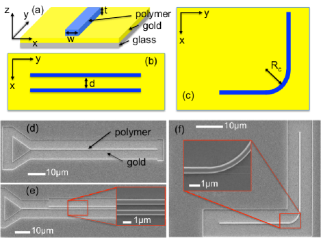
Figure 1: (a) Schematic view of a basic DLSPPW with a width $w$ of 600 nm and thickness $t$=560 nm. (b) Schematic view of two coupled waveguides separated by a gap $d$. (c) Schematic view of a curved waveguide with a bend radius $R_{c}$. (d), (e) and (f) are scanning electron micrographs of typical devices corresponding to the configurations (a), (b), and (c), respectively.

II.2 Characterization setup

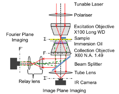
Figure 2: Schematic of the leakage radiation microscope used in this study. Launching of the plasmon mode in the waveguides is obtained by focusing a laser operating at $\lambda$=1510 nm with a long working distance objective. Surface plasmon leakages are collected by an oil immersion objective and are imaged on two cameras placed at the conjugated image (field) plane and Fourier (aperture) plane, respectively.

Optical characterization is performed by using a home-made leakage radiation microscope (LRM). The principle of this method is only recalled here, more detailed can be found in the review by Drezet et al.Drezet et al. (2008). The schematic view of our experimental set-up is illustrated in Fig. 2. An incident tunable laser beam (fixed at $\lambda$=1510 nm hereafter) is focused by a 100 $\times$ microscope objective on the extremity of a DLSPP waveguide. The sharp discontinuity defined by the polymer structure acts a local scatterer and produces a spread of wave-vectors, some of which resonant with the surface plasmon modes supported by the geometry. By controlling the incident polarization parallel to the longitudinal axis of the waveguide Frisbie et al. (2010), the DLSPPW mode can thus be readily excited. Leakage radiation microscopy (LRM) provides a far-field imaging technique to directly visualize surface plasmon propagation and investigate its fundamental properties Hecht et al. (1996); Bouhelier et al. (1999). This method relies on the collection of radiation losses occurring in the waveguide during propagation. These losses are emitted in the substrate at an angle phase-matched with the in-plane wave-vector of the SPP mode. In our LRM, the plasmon radiation losses are collected by an oil-immersion objective with a numerical aperture (N.A.) of 1.49. A tube lens focuses the leakages in an image plane (IP) conjugated with the object plane where an InGaAs infrared camera is recording the two-dimensional intensity distribution. Images recorded at this plane provide direct information about the propagation of the surface plasmon mode developing in the DLSPPW. To complete the analysis, we have also used the Fourier transforming property of the objective lens to access the wave-vector distribution of the emitted light. The angular distribution of the rays radiated in the substrate and collected by the objective lens is transformed to a lateral distribution at the objective back focal plane. Quantitative measurement of the complex surface plasmon wave-vector, or equivalently its complex effective index, consists at measuring the radial distance of the rays with respect to the optical axis. Access to momentum space was done by inserting a beam splitter in the optical path and a set of Fourier transforming relay lens. The lenses are forming an image conjugated with back focal plane of the objective. This Fourier plane (FP) contains the two-dimensional wave-vector distribution of the leakage radiation and momentum-space spectroscopy can thus be readily performed.

II.3 Calibrating leakage radiation images

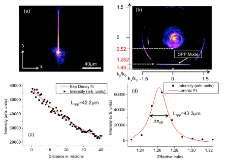
Figure 3: (a) Intensity distribution recorded at the image plane of a surface plasmon mode propagating along a straight DLSPPW. The excitation spot is readily visible at the lower portion of the waveguide. (b) Corresponding wave-vector distribution. The central disk represents to the numerical aperture of the illumination objective (0.52). The DLSPP mode is recognized as a bright line at constant $k_{y}/k_{x}$ (arrow). (c) Exponential fit of the experimental decaying plasmon intensity along the waveguide leading to a $L_{spp}$=42.2 $\mu$m. (d) Lorentzian fit of the FP plasmon mode signature centered at $\beta^{\prime}/k_{o}$=1.262. The full with at half maximum $\Delta n_{eff}$ is inversely proportional to $L_{spp}$.

Figures 3(a) and (b) show images of the leakage radiation intensity of a single-mode DLSPPW recorded in the conjugated image and Fourier planes, respectively. The plasmon mode is launched at the bottom of the structure and propagates up the waveguide with an exponentially decaying intensity. The image of Fig. 3(b) is a direct measurement of the wave-vector content of the intensity distribution shown in Fig. 3(a). For both FP and IP images, a calibration was performed prior to any data extraction. For calibrating IP images, we used the known waveguide length as a standard. With the system magnification one pixel represents $\simeq$0.6 $\mu$m. For FP images, the $N.A.$ of the objective was used to calibrate $k_{x}$ and $k_{y}$ axes. The largest ring in Fig. 3(b) represents the $N.A.$=1.49 specified by the manufacturer. The central disk is the numerical aperture of the $\times 100$ excitation objective at $N.A.$=0.52. One pixel provides a $\Delta N.A.\simeq$ 0.012.

The DLSPPW mode propagating along this straight waveguide presented in Fig. 3 can be defined by two parameters: its effective index $n_{eff}$ and propagation length $L_{spp}$. $n_{eff}$ is expressed by the phase constant $\beta^{\prime}$ and reads $n_{eff}=\beta^{\prime}/k_{o}$ where $k_{o}=2\pi/\lambda$. The propagation length $L_{spp}=(2\beta^{\prime\prime})^{-1}$ where $\beta^{\prime\prime}$ is the attenuation constant of the plasmon mode. A complex propagation constant is then evaluated from these two constants: $\beta=\beta^{\prime}+i\beta^{\prime\prime}$.

$L_{spp}$ can be directly extracted from direct-space image by fitting an exponential decay of the intensity along the waveguide $I=I_{0}\exp(-y/L_{spp})$. Here a $L_{spp}$=42.2 $\mu$m is determined from the fit to the experimental data illustrated in Fig. 3(c). Experimentally, the FP image displayed in Fig. 3(b) contains more information than a direct space image since the real part and imaginary part of the effective index can be directly measured. The signature of the mode is represented by a single line at a constant $n_{eff}$=$k_{y}/k_{o}$=1.262$\pm$0.006. The intensity measured along $k_{y}/k_{o}$ at $k_{x}$=0 is related to the surface plasmon through the following formula Grandidier et al. (2009): $I(k_{x},k_{y})\propto|\widetilde{H}_{0}(k_{x})|^{2}/[(k_{y}-\beta^{\prime})^{2}+(1/2L_{spp})^{2}]$. $\widetilde{H}_{0}(k_{x})$ is the $k_{x}$-Fourier transform of the guided magnetic field at the objective focal point. The imaginary part of the effective index is also estimated precisely through a Lorentzian fit. The width $\Delta n_{eff}$ of the $\beta^{\prime}/k_{o}$ line is a measure of the losses experienced by the plasmon mode and is thus inversely proportional to its propagation length $L_{spp}$ Raether (1988). We obtain from the FP image a $L_{spp}$=43.3 $\mu$m in fairly good agreement with $L_{spp}$=42.2 $\mu$m measured from direct-space analysis.

III Momentum-space spectroscopy of linear DLSPPW couplers

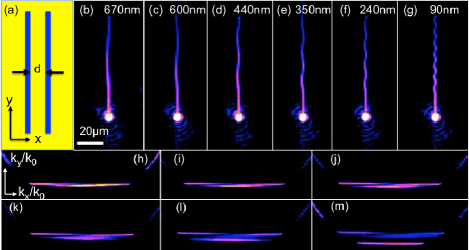
Figure 4: (a) Schematic of a linear DLSPPW coupler. (b) to (g) are direct-space images of the intensity distribution in linear DLSPPW couplers with edge-to-edge distance $d$ equals to 670 nm, 600 nm, 440 nm, 350 nm, 240 nm and 90 nm respectively. (h) to (m) are the corresponding wave-vector distributions unambiguously demonstrating the degeneracy lift of the coupled waveguides for small values of $d$. The images were cropped to display only the lower part of the Fourier plane.

We now demonstrate the added-value of performing momentum-space leakage radiation spectroscopy of a classical integrated plasmonic routing device: a linear DLSPPW coupler Steinberger et al. (2007); Krasavin and Zayats (2008); Chen et al. (2009); Colas des Francs et al. (2009). The linear coupler geometry illustrated in Fig. 4(a) consists of two parallel and identical DLSPP waveguides separated by an edge-to-edge distance $d$ varying from 670 nm to 90 nm. This elementary configuration is well-known from coupled-mode theory Yariv (2000). When the gap distance $d$ is reduced the degenerate modes propagating in the uncoupled waveguides are split into symmetric and antisymmetric modes. New propagation constants $\beta^{\prime}_{s}$ and $\beta^{\prime}_{as}$, respectively are thus characterizing the symmetric mode and the antisymmetric mode, respectively, and they critically depend on $d$. A beating of these two modes can be observed in leakage radiation microscopy Chen et al. (2009); Colas des Francs et al. (2009) where a mode propagating in one waveguide can be totally transferred to the second after a coupling distance $L_{c}$ Holmgaard et al. (2009). Figures 4(b)-(g) qualitatively show the evolution of the beating pattern and the coupling distance $L_{c}$ for decreasing separation distances $d$. More interesting are the corresponding wave-vector distributions depicted in the series of FP images in Figs. 4(h) to (m). When the DLSPPWs are weakly coupled ($d$=670 nm), the Fourier content of Fig. 4(h) strongly resembles that of a single DLSPP mode already shown in Fig. 3(b). When $d$ is reduced, a clear splitting of the modes is observed indicative of a strong interaction between the waveguides. The parity of the modes can be readily determined from e.g. Fig. 4(m). The asymmetric mode has an odd parity with two maxima centered on each side of $k_{y}/k_{o}$ axis.

Figure 5 illustrates the benefit of performing momentum-space spectroscopy described here. Figures 5(a) and (b) are leakage radiation images recorded at the conjugated Fourier plane and image plane for a linear coupler with $d$=440 nm, respectively. The effective indices of the symmetric $n_{eff}^{s}$ and antisymmetric $n_{eff}^{as}$ modes are evaluated by Lorentzian fits of crosscuts of the momentum distribution along the $k_{y}/k_{o}$ axis marked by the circles in Fig. 5(a). $n_{eff}^{as}$ was evaluated at two different wave-vector positions with respect to the $k_{y}/k_{o}$ axis, labeled as $n_{eff}^{as}$ and $n_{eff}^{as^{\prime}}$. The fits to the data are represented in Figs. 5(c) and (d) for the antisymmetric mode leading to $n_{eff}^{as}\simeq n_{eff}^{as^{\prime}}$=1.260$\pm$0.006. The effective index of the symmetric mode is measured at $n_{eff}^{s}$=1.310$\pm$0.006 (Fig. 5(e)).

The coupling length $L_{c}$ can now be evaluated using the following relation Holmgaard et al. (2009)

$$L_{c}=\frac{\pi}{|\beta^{\prime}_{s}-\beta^{\prime}_{as}|},$$ (1)

where $\beta^{\prime}_{s}=k_{o}\times n_{eff}^{s}$ and $\beta^{\prime}_{as}=k_{o}\times n_{eff}^{as}$ . Then

$$L_{c}=\frac{\lambda_{0}}{2|n_{eff}^{s}-n_{eff}^{as}|}=15.2\rm{\mu m}.$$ (2)

This procedure was repeated for the different DLSPPW separation distances $d$. The extracted values of the split modes and coupling length $L_{c}$ are reported in Table 1. $L_{c}$ was estimated taking into account an average value of $n_{eff}^{as}$ and $n_{eff}^{as^{\prime}}$. For comparison purposes, $L_{c}$ was also determined by analyzing the beating pattern recorded in the image plane (Fig. 5(b)). A longitudinal cross-section of the leakage intensity taken along each DLSPPWs is shown in Fig. 5(f) for $d$=440 nm. The transfer of the mode between the two waveguides is obtained after $L_{c}\sim$16 $\mu$m. Within our pixel resolution, this value compares well with the $L_{c}$ determined by the analysis of the degeneracy lift of the effective indices by Eq. 2. The advantage of a momentum-space spectroscopy is that, unlike near-field measurement Steinberger et al. (2007); Holmgaard et al. (2009), the effective indices can be directly measured and mode symmetry visualized Grandidier et al. (2008); Frisbie et al. (2010). $L_{c}$ inferred from direct plane analysis only provides the difference between the two propagation constants $|\beta^{\prime}_{s}-\beta^{\prime}_{as}|$ without discriminating the symmetric mode from the antisymmetric one.

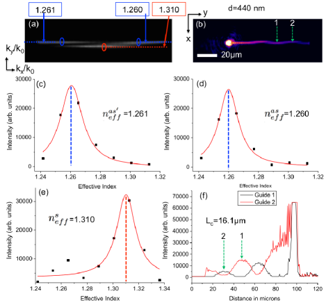
Figure 5: (a) and (b) are the respective leakage radiation Fourier and image planes obtained from a linear DLSPPW coupler with $d$=440 nm. (c) and (d) are Lorentzian fits of the asymmetric mode at the location marked by the circle in (a). (e) is a Lorentzian fit of the symmetric mode. (f) Longitudinal intensity cross sections taken along the two coupled waveguides in (b) showing the energy transfer from one DLSPPW to the other defining the coupling length $L_{c}$.

$d$ [nm]	$n_{eff}^{as}$	$n_{eff}^{as^{\prime}}$	$n_{eff}^{s}$	$L_{c}$ [$\mu$m](FP)	$L_{c}$ [$\mu$m](IP)
090	1.230	1.234	1.403	4.4	4.3
240	1.241	1.244	1.343	7.5	7.7
350	1.252	1.254	1.316	12.0	11.8
440	1.260	1.261	1.310	15.2	16.1
600	1.262	1.263	1.299	20.6	21.1
670	1.271	1.271	1.294	32.8	31.4

Table 1: Measured values of the effectives indices of the asymmetric and symmetric modes and estimated coupling length $L_{c}$ for linear DLSPPW couplers with different edge-to-edge separation $d$. $L_{c}$ values were estimated independently by momentum-space spectroscopy and direct-plane analysis.

To confirm these experimental results, we numerically simulated linear DLSPPW couplers with the commercial Finite-Element mode solver COMSOL. The optical index of the PMMA waveguide is $n_{pmma}=1.535$ and that of the gold layer is $n_{gold}=0.536+i9.5681$ at $\lambda$=1510 nm Palik (1998). The transversal electric field distribution of the asymmetric and symmetric mode are shown Figs. 6 (a) and (b) for $d$=400 nm. Figure 6(c) provides a comparison of the evolution of the degeneracy lift with separation distance $d$. The measured data quantitatively reproduce the response of the simulated device.

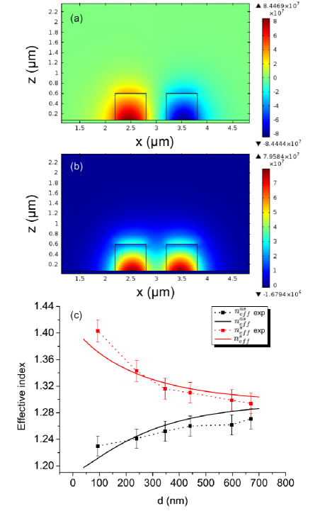
Figure 6: (a) and (b) are the electric field profiles of the asymmetric and symmetric modes propagating in two coupled DLSPPWs separated by $d$=400 nm. (c) Comparison between the experimental splitting and the calculated values for various coupling distances $d$.

IV Momentum-space spectroscopy of curved DLSPPWs

IV.1 Experimental images

In this section, we investigate the momentum distribution of another well-known basic routing element: 90^∘ curved waveguides. This DLSPPW structure has been extensively studied by various groups and the effect of bend radius on the overall losses is well understood Marcatili (1969); Krasavin and Zayats (2008); Dikken et al. (2010); Song et al. (2010); Yang et al. (2012). By performing momentum-space spectroscopy of the supported mode, we visualize and analyze the wave-vector content of the bend section for this routing device. We demonstrate the limitations of momentum-space spectroscopy to extract modal properties of this elementary building block. The curved DLSPPW is composed of two $L$=30 $\mu$m long straight waveguides with $w$=600 nm. These two input and output waveguides are linked by a circular $90^{\circ}$ bend section of radius $R_{c}$. Bent DLSPPWs with $R_{c}$ ranging from 5 $\mu$m to 19 $\mu$m were fabricated. The leakage intensity distribution image of a $R_{c}$=19 $\mu$m curved waveguide is shown Fig. 7(a). The corresponding wave-vector distribution is depicted in Fig 7(b). The two straight lines at $k_{x}$ and $k_{y}$ constant are related to the mode propagating along the $y$ and $x$-oriented waveguides, respectively. The line at $k_{x}$=constant is the input waveguide. This Fourier plane shows additional signatures such as the illumination wave-vector span (central disk) and planar plasmon modes supported by the Au/air or Au/PMMA taper interfaces. Of particular interest here is the Fourier signature of the bent section of the waveguide visible as an arc of circle linking the two $k_{x}$ and $k_{y}$ lines.

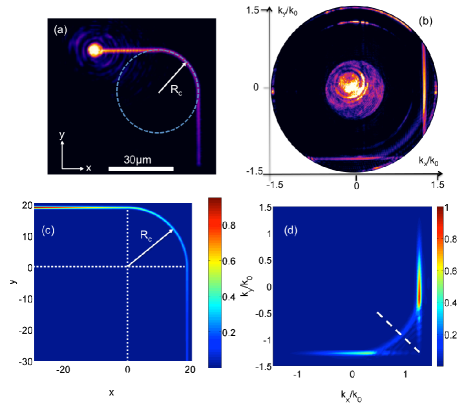
Figure 7: (a) and (b) Leakage radiation image of a bent waveguide with $R_{c}$=19 $\mu$m and its corresponding wave-vector distribution, respectively. The Fourier content of the curved section is appearing as an arc linking the two $k_{x}$ and $k_{y}$ lines. (c) and (d) Computed intensity of the mode propagating in the routing element and its corresponding wave-vector distribution, respectively.

IV.2 Fourier plane model

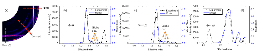
Figure 8: (a) Experimental momentum-space image of a $R_{c}=19~{}\mu$m bend waveguide. The dashed lines indicate the position of the momentum profile in the following graphs. (b) (c) and (d) show the comparison of the calculated and experimental wave-vector distributions along the $k_{x}$, $k_{y}$ and -$\pi/4$ axis, respectively.

Instead of full numerical simulations, we propose in the following a simple analytical model that explains the main features of the measured Fourier plane images. To this aim, we approximated the mode that propagates in the bend structure by a gaussian profile with a finite propagation length. The characteristics of the gaussian profile was defined by the experimental data obtained from a straight waveguide; namely $n_{eff}$=1.262 and $L_{spp}$=42.2 $\mu$m. The mode width was fixed at $w_{0}$=500 nm according to the analysis of Holmgaard and Bozhevolnyi Holmgaard and Bozhevolnyi (2007).

The magnetic field is written as follow:

• input straight guide ($-L<x<0$, $y>0$)

  $$H_{y}(x,y)=H_{o}\exp\left[\frac{-(y-R_{c})^{2}}{w_{0}^{2}}\right]\exp[i\beta x]\,,$$ (3)

  $$=H_{o}\exp\left[\frac{-(y-R_{c})^{2}}{w_{0}^{2}}\right]\exp[in_{eff}k_{o}x]\exp[-x/2L_{spp}]\,,$$

• circular portion ($x>0$, $y>0$)

  $$H_{r}(r,\theta) = H_{o}\exp[-L/2L_{spp}]$$

  $$\exp\left[\frac{-(r-R_{c})^{2}}{w_{0}^{2}}\right]\exp[ik_{b}R_{c}\theta]\,,$$

  where $r=\sqrt{x^{2}+y^{2}}$, $\theta=\arctan{(x/y)}$ and $k_{b}$ is the complex wave-vector of the mode in the curved section.

• output straight guide ($x>0$, $-L<y<0$)

  $$H_{x}(x,y) = H_{o}\exp\left[\frac{-(x-R_{c})^{2}}{w_{0}^{2}}\right]\exp[-L/2L_{spp}]$$

  $$\exp[-R_{c}\pi/4L_{spp}]\exp[in_{eff}k_{o}y]\exp[-y/2L_{spp}]\,.$$

The momentum representation $\tilde{H}(k_{x},k_{y})$ was obtained by a Fourier transform

$$\tilde{H}(k_{x},k_{y})=\int_{-L}^{R_{c}+3\times w_{0}}\int_{-L}^{R_{c}+3\times w_{0}}\!H(x,y)\,$$ (6)

$$\exp\left[-i(k_{x}x+k_{y}y)\right]\mathrm{d}x\mathrm{d}y.$$

where the integration window is truncated to limit the calculation on the mode extension. Outside this area, the mode profile vanishes so that its contribution to the Fourier transform is negligibly small.

To simulate the curved DLSPPW, we maintained the complex propagation constant in the curved section equal to that of the straight waveguides ($k_{b}=\beta$). This assumption remains valid for $R_{c}>R_{l}$ where $R_{l}$ is the limiting radius where bend losses can be neglected. $R_{l}$ have been recently numerically estimated for DLSPPW Song et al. (2010) confirming an analytical expression historically used for standard optical waveguides Marcatili (1969)

$$R_{l}>\frac{24\pi^{2}|w_{3}|^{3}}{\lambda^{2}}.$$ (7)

Here $w_{3}$ corresponds to the length over which the field outside of the waveguide decays by $1/e$. With $w_{3}\simeq w_{0}$, $R_{l}\simeq$ 13 $\mu$m. When the radius is below $R_{l}$, bending losses are induced by a radial displacement of the mode profile with respect to the waveguide axis Song et al. (2010). This displacement pushes the field outside the waveguide leading to a lower phase velocity and a modification of the effective index Hunsperger (1995).

Considering curvature loss as an additional exponential decay is a good approximation to quantify the total loss induced by the bend and estimate the transmission of the 90^∘ waveguide. However, this approximation is not representative of the real shape of the field along the bend and consequently cannot be used to model Fourier images of the kind displayed in Fig. 7(b).

For $R_{c}>R_{l}\simeq$13 $\mu$m, we show that the propagation and momentum-space representations simulated with these basic assumptions (Figs. 7(c) and (d)) reproduces the experimental observations of Figs. 7(a) and (b). We compare the profile of the calculated Fourier transform (Fig. 7(d)) to the experimental wave-vector distribution (Fig. 7(b)) by extracting momentum profiles at different radial coordinates indicated in Fig. 8(a) for $R_{c}$=19 $\mu$m. Figures 8(b), (c) and (d) show the calculated and experimental wave-vector distributions taken along the $k_{x}$ and $k_{y}$ axis and at -$\pi/4$, respectively. The position and width of the calculated wave-vector profiles are in very good agreement with the measured data validating thus our preliminary assumptions. Some extra signatures are visible on the experimental cuts: a peak at 1.49 in Fig. 8(b) corresponds to the numerical aperture of the collection objective, and the contribution of the surface plasmon excited in the nearby gold film is visible at 1.08 in Fig. 8(d). Noticeable also is the presence of Gibbs oscillations revealed by this momentum-space spectroscopy (arrows Figs. 8 (b) and (c)) . The origin of these oscillations in reciprocal space is discussed below.

IV.3 Analytical development

In order to provide analytical expressions and propose a simple physical understanding of the measured Fourier images, we simplified further the model. We consider each part of the waveguide (straight and bend) independently from each others. The straight parts are approximatively 30 $\mu$m long, a length smaller than the longitudinal decay of the supported mode ($L_{spp}$=42 $\mu$m). If we consider only the field in the input straight waveguide along the $x$ coordinate, the Fourier transform of the magnetic field written in Eq. 3 reads

$$\tilde{H}_{y}(k_{x})=H_{o}\int_{-L}^{0}\!\exp[i(\beta-k_{x})x]\,\mathrm{d}x\,,$$ (8)

where we neglected the $y$-gaussian profile for the sake of clarity but this could be easily considered. Then the intensity in the Fourier plane along $k_{x}$ direction writes

$$|\tilde{H}_{y}(k_{x})|^{2}=|H_{o}|^{2}\frac{1-2e^{-\beta^{\prime\prime}L}\cos((\beta^{\prime}-k_{x})L)+e^{-2\beta^{\prime\prime}L}}{(\beta^{\prime}-k_{x})^{2}+\beta^{\prime\prime 2}}$$ (9)

If $L\rightarrow\infty$ then $|\tilde{H}_{y}(k_{x})|^{2}\rightarrow 1/[(\beta^{\prime}-k_{x})^{2}+\beta^{\prime\prime 2}]$ and follows a Lorentzian profile, as expected. If the straight part length $L$ is smaller than $L_{spp}$, the resulting Fourier transform is not simply defined by a Lorentzian function. Because of the finite integration limit, extra oscillations are becoming visible (Gibbs oscillations) as illustrated in Figs. 8(b) and (c). For long waveguide (as in Fig. 3(a) where $L>L_{spp}$), no oscillation of the wave-vector distribution is observed. Figure 9 shows the impact of the integration boundaries $L$ on the momentum space representation of a single straight waveguide for a fixed propagation length of 40 $\mu$m. There is a perfect agreement between the numerically calculated Fourier transform and its analytical solution given by Eq. 9. For integration boundaries greater than the propagation length the two calculations match with the Lorentz function generally used.

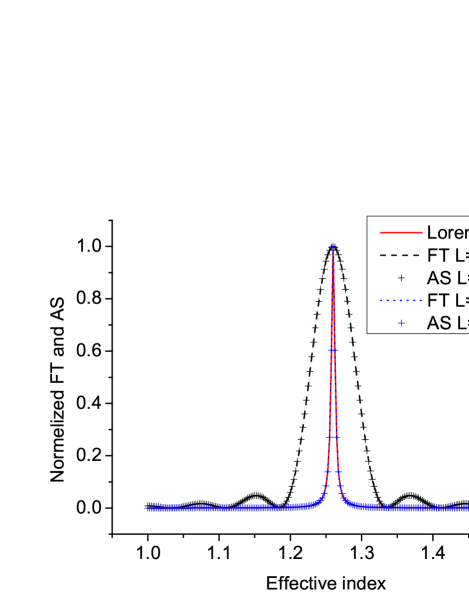
Figure 9: Effect of the DLSPPW length on Fourier plane calculations. Dashed lines: calculated Fourier plane (FT) cross section for $L=0.5\times L_{spp}$ and $L=10\times L_{spp}$. Crosses: analytical solutions (AS) calculated from Eq. 9 with the same integration boundaries. Red solid line: calculated Lorentzian profile of the wave-vector distribution of a plasmon mode with a propagation length of 40 $\mu$m. When $L<L_{spp}$ Gibbs oscillations and widening of the wave-vector content occur.

Since the momentum space representation of a straight waveguide can be expressed for any integration boundaries, we now look for the expression of a curved waveguide alone. On Fig. 8 (d), the $-\pi/4$ profile shows the experimental momentum space of a $90^{\circ}$ curved waveguide linked by an input and an output waveguide. We approximate in the following a solution considering a fully symmetric configuration consisting of a lossless circular waveguide. Losses are omitted to maintain the radial symmetry valid between [0;2$\pi$]. The Fourier transform in a $360^{\circ}$ bend can be expressed in polar coordinates as

$$\tilde{H}(k_{r},\phi)=\int_{0}^{\infty}\int_{0}^{2\pi}\!H_{r}(r,\theta)e^{-2i\pi k_{r}r\cos(\theta-\phi)}r\,\mathrm{d}r\mathrm{d}\theta.$$ (10)

$H_{r}(r,\theta)$ is given by Eq. • ‣ IV.2. Since this function is periodic with respect to $\theta$ between [0;2$\pi$], we can expand $H_{r}(r,\theta)$ in a Fourier series:

$$H_{r}(r,\theta)=\sum_{n=-\infty}^{+\infty}{H_{n}(r)}e^{in\theta},$$ (11)

where the $n^{{\rm th}}$ harmonic is

$$H_{n}(r) = \frac{1}{2\pi}\int_{-\pi}^{\pi}{H_{r}(r,\theta)}e^{-in\theta}\mathrm{d}\theta$$

$$= e^{\left[\frac{-(r-R_{c})}{w_{0}^{2}}\right]}{\rm sinc}(k_{b}R_{c}\pi-n\pi).$$

The Fourier transform of the field (Eq. 10) can now be written as follow

$$\tilde{H}_{n}({k}_{r},\phi)=\sum_{n=-\infty}^{+\infty}{(-i)^{n}}e^{i\phi n}2\pi\int_{0}^{\infty}{rH_{n}(r)J_{n}(2\pi k_{r}r)}dr,\\$$ (13)

$$\tilde{H}_{n}({k}_{r},\phi)=\sum_{n=-\infty}^{+\infty}{h_{n}}{f_{n}({k}_{r},\phi)},$$ (14)

with

$${h_{n}}={\rm sinc}(k_{b}R_{c}\pi-n\pi),$$ (15)

and

$$f_{n}({k}_{r},\phi)={(-i)^{n}}e^{i\phi n}2\pi\int_{0}^{\infty}{re^{\left[\frac{-(r-R_{c})}{w_{0}^{2}}\right]}J_{n}(2\pi k_{r}r)}dr.$$

$J_{n}(2\pi k_{r}r)$ is the Bessel function of the first kind of $n^{{\rm th}}$ order. Further simplification can be achieved by extracting the main $n^{{\rm th}}$ harmonic $h_{n}$ of the series. It is deduced from Eq. 15 and is such that

$$k_{b}R_{c}\pi-n\pi=0<=>n=k_{b}R_{c}.$$ (16)

Therefore the Fourier series is dominated by the harmonic integer that is the closest to the product $k_{b}R_{c}$.

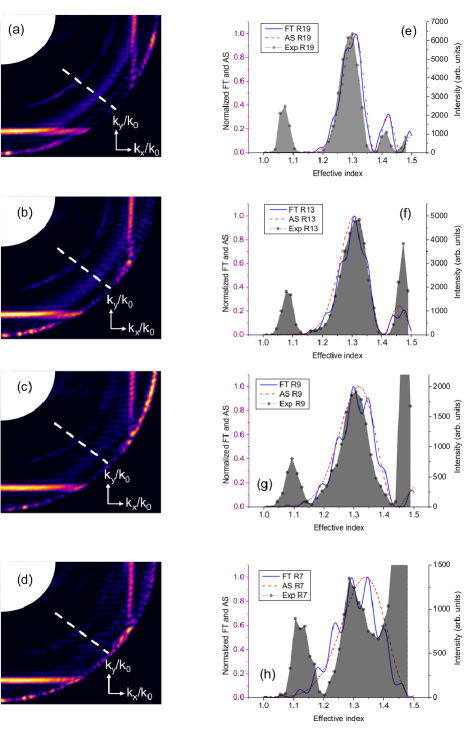
Figure 10: (a-d) Selected region of interest of the experimental momentum-space images for curved waveguides with $R_{c}$=19 $\mu$m, 13 $\mu$m, 9 $\mu$m, and 7 $\mu$m, respectively. (e) to (h) Experimental profiles (shaded areas) of the wave-vector distribution taken along the dashed line in (a) to (d). The solid blue lines are the calculated profiles using Eq. 6 already reported in Fig. 8. The red dashed lines show the analytical solutions obtained with the $n^{{\rm th}}$ order rendering the best agreement with the data. $n$=100, 68, 43, and 37, respectively.

Figure 10 illustrates a comparison between the experimental data extracted from momentum-space spectroscopy, the Fourier calculations derived from Eq. 6 already used in Figure 8, and the analytical approximation discussed above. The experimental Fourier planes of Figs. 10 (a) to (d) only show the region of interest for four different radii. The corresponding wave-vector profiles extracted and calculated at $-\pi$/4 (dashed lines in figure 7(d)) are plotted in the graphs of Figs. 10 (e) to (h). For radius $R_{c}>R_{l}$, the Fourier calculations and the analytical solutions are in good agreement with the experimental data. For large radii the signature of the bend in momentum space is defined only by the phase difference $k_{b}(2\pi R_{c})=n2\pi$. This corresponds to resonance condition of a ring resonator.

Experimentally, the periodic condition on $\theta$ is not respected since the structure considered is formed by an arc of circle. Nonetheless, using the $n=100^{{\rm th}}$ order of the Bessel function in Eq.  13 for $R_{c}$=19 $\mu$m and the $68^{{\rm th}}$ order for $R_{c}$=13 $\mu$m the experimental data and the calculated Fourier transform can be well reproduced (Figs. 10 (e) and (f)). For radius $R_{c}<R_{l}$ , the calculated profiles deduced from Eq. 6 and from the $n=47^{{\rm th}}$ and $n=37^{{\rm th}}$ orders for $R_{c}$=9 $\mu$m and $R_{c}$=7 $\mu$m, respectively are deviating from the experimental cross-cuts (Figs. 10 (g) and (h)). This disagreement is expected since none of the two models (Fourier transform and analytical approximation) are including bending loss.

V conclusion

By using dual-plane leakage radiation microscopy we have fully quantified the key parameters characterizing two important dielectric-loaded surface plasmon polariton routing devices: linear couplers and 90^∘ curved waveguides. We unambiguously demonstrated the added-value of performing momentum-space spectroscopy. The degeneracy lift for strongly coupled waveguides and the symmetry of the split modes can be directly visualized and quantified. The wave-vector distribution associated to the curved section of the waveguide was also readily observed. We developed a numerical and an analytical analyzis to understand the experimental momentum distribution. We found that for large radii (vanishing bending loss), we can link the plasmon signature in Fourier space with the geometrical and modal properties of the bend structure. The radial dependence of the wave-vector distribution is governed by the phase difference $k_{b}(2\pi R_{c})$. For smaller radii of curvature the bend loss need to be accounted for by developing an approach including realistic field shape.

VI Acknowledgments

This work was funded by the European FP7 research program PLATON, Contract Number 249135 and the European Research Council grant agreement number 306772, the regional council of Burgundy under the program PARI SMT3 and the Labex ACTION. S. Lachèze is acknowledged for participating at the early stage of this work, with the support of Burgundy Region and CEA Leti Carnot funding.

References

- Hohenau et al. (2005) A. Hohenau, J.R.Krenn, A. Stepanov, A. Drezet, H. Ditlbacher, B. Steinberger, A. Leitner, and F. Aussenegg, Opt. Lett. 30, 893 (2005).
- Holmgaard et al. (2008a) T. Holmgaard, S. I. Bozhevolnyi, L. Markey, and A. Dereux, Appl. Phys. Lett. 92, 011124 (2008a).
- Grandidier et al. (2008) J. Grandidier, S. Massenot, G. Colas des Francs, A. Bouhelier, J.-C. Weeber, L. Markey, and A. Dereux, Phys. Rev. B 78, 245419 (2008).
- Briggs et al. (2010) R. M. Briggs, J. Grandidier, S. P. Burgos, E. Feigenbaum, and H. A. Atwater, Nano Lett. 10, 4851 (2010).
- Kalavrouziotis et al. (2012) D. Kalavrouziotis, S. Papaioannou, K. Vyrsokinos, A. Kumar, S. I. Bozhevolnyi, K. Hassan, L. Markey, J.-C. Weeber, A. Dereux, G. Giannoulis, D. Apostolopoulos, H. Avramopoulos, and N. Pleros, IEEE Phot.Tech. Lett. 24, 1036 (2012).
- Papaioannou et al. (2011) S. Papaioannou, K. Vyrsokinos, O. Tsilipakos, A. Pitilakis, K. Hassan, J.-C. Weeber, L. Markey, A. Dereux, S. I. Bozhevolnyi, A. Miliou, E. E. Kriezis, and N. Pleros, IEEE J. Light.Tech. 29, 3185 (2011).
- Grandidier et al. (2010) J. Grandidier, G. Colas des Francs, L. Markey, A. Bouhelier, S. Massenot, J.-C. Weeber, and A. Dereux, Appl. Phys. Lett. 96, 063105 (2010).
- Grandidier et al. (2009) J. Grandidier, G. Colas des Francs, S. Massenot, A. Bouhelier, L. Markey, J.-C. Weeber, C. Finot, and A. Dereux, Nano Lett. 9, 2935 (2009).
- Gosciniak et al. (2010) J. Gosciniak, S. I. Bozhevolnyi, T. B. Andersen, V. S. Volkov, J. Kjelstrup-Hansen, L. Markey, and A. Dereux, Opt. Express 18, 1207 (2010).
- Randhawa et al. (2012) S. Randhawa, S. Lachèze, J. Renger, A. Bouhelier, R. Espiau de Lamaestre, A. Dereux, and R. Quidant, Opt. Express 20, 2354 (2012).
- Perron et al. (2011) D. Perron, M. Wu, C. Horvath, D. Bachman, and V. Van, Opt. Lett. 36, 2731 (2011).
- Krasavin et al. (2011) A. V. Krasavin, S. Randhawa, J.-S. Bouillard, J. Renger, R. Quidant, and A. V. Zayats, Opt. Express 19, 25222 (2011).
- Hassan et al. (2011) K. Hassan, J.-C. Weeber, L. Markey, and A. Dereux, J. Appl. Phys. 110, 023106 (2011).
- Hecht et al. (1996) B. Hecht, H. Bielefeldt, L. Novotny, Y. Inouye, and D. W. Pohl, Phys. Rev. Lett. 77, 1889 (1996).
- Holmgaard et al. (2008b) T. Holmgaard, S. Bozhevolnyi, L. Markey, A. Dereux, A. V. Krasavin, P. Bolger, and A. Zayats, Phys. Rev. B 78, 165431 (2008b).
- Steinberger et al. (2007) B. Steinberger, A. Hohenau, H. Diltlbacher, F. R. Aussenegg, A. Leitner, and J. R. Krenn, Appl. Phys. Lett. 91, 081111 (2007).
- Krishnan et al. (2010) A. Krishnan, C. J. Regan, L. G. de Peralta, and A. A. Bernussi, Appl. Phys. Lett. 97, 231110 (2010).
- Berthelot et al. (2011) J. Berthelot, A. Bouhelier, G. Colas des Francs, J.-C. Weeber, and A. Dereux, Opt. Express 19, 5303 (2011).
- Regan et al. (2012) C. J. Regan, O. Thiabgoh, L. G. de Peralta, and A. Bernussi, Opt. Express 20, 8658 (2012).
- Holmgaard and Bozhevolnyi (2007) T. Holmgaard and S. I. Bozhevolnyi, Phys. Rev. B 75, 245405 (2007).
- Drezet et al. (2008) A. Drezet, A. Hohenau, D. Koller, A. Stepanov, B. S. H. Ditlbacher, F. Aussenegg, A. Leitner, and J. Krenn, Mat. Sci. Eng. B 148, 220 (2008).
- Frisbie et al. (2010) S. Frisbie, C. Chesnutt, J. Ajimo, A. Bernussi, and L. G. de Peralta, Opt. Comm. 283, 5255 (2010).
- Bouhelier et al. (1999) A. Bouhelier, T. Huser, H. Tamaru, H.-J. Güntherodt, and D. W. Pohl, J. Microsc. 194, 571 (1999).
- Raether (1988) H. Raether, Surface Plasmons on Smooth and Rough Surfaces and on Gratings, Springer Tracts in Modern Physics, Vol. 111 (Springler-Verlag, 1988).
- Krasavin and Zayats (2008) A. V. Krasavin and A. V. Zayats, Phys. Rev. B 78, 045425 (2008).
- Chen et al. (2009) Z. Chen, T. Holmgaard, S. Bozhevolnyi, A. V. Krasavin, A. V. Zayak, L. Markey, and A. Dereux, Opt. Lett. 34, 310 (2009).
- Colas des Francs et al. (2009) G. Colas des Francs, J. Grandidier, S. Massenot, A. Bouhelier, J.-C. Weeber, and A. Dereux, Phys. Rev. B 80, 115419 (2009).
- Yariv (2000) A. Yariv, Electron. Lett. 36, 321 (2000).
- Holmgaard et al. (2009) T. Holmgaard, Z. Chen, S. I. Bozhevolnyi, L. Markey, and A. Dereux, J. Ligthw. Tech. 27, 5521 (2009).
- Palik (1998) E. D. Palik, ed., Handbook of optical constants of solids (Academic press, 1998).
- Marcatili (1969) E. A. Marcatili, Bell Syst. Tech. J. 48, 2103 (1969).
- Dikken et al. (2010) D. J. Dikken, M. Spasenović, E. Verhagen, D. van Oosten, and L. K. Kuipers, Opt. Express 18, 16112 (2010).
- Song et al. (2010) S. Yue, Z. Li, J.-J. Chen, and Q.-H. Gong, Chin. Phys. Lett. 27, 027303 (2010).
- Yang et al. (2012) C. Yang, E. J. Teo, T. Goh, S. L. Teo, J. H. Teng, and A. A. Bettiol, Opt. Express 20, 23898 (2012).
- Hunsperger (1995) R. G. Hunsperger, Integrated Optics: Theory and Technology (Springer-Verlag Berlin Heidelberg, 1995).