Protostellar Disk Evolution Over Million-Year Timescales with a Prescription for Magnetized Turbulence

Abstract

Magnetorotational instability (MRI) is the most promising mechanism behind accretion in low-mass protostellar disks. Here we present the first analysis of the global structure and evolution of non-ideal MRI-driven T-Tauri disks on million-year timescales. We accomplish this in a 1+1D simulation by calculating magnetic diffusivities and utilizing turbulence activity criteria to determine thermal structure and accretion rate without resorting to a 3-D magnetohydrodynamical (MHD) simulation. Our major findings are as follows. First, even for modest surface densities of just a few times the minimum-mass solar nebula, the dead zone encompasses the giant planet-forming region, preserving any compositional gradients. Second, the surface density of the active layer is nearly constant in time at roughly 10 g cm^-2, which we use to derive a simple prescription for viscous heating in MRI-active disks for those who wish to avoid detailed MHD computations. Furthermore, unlike a standard disk with constant-$\alpha$ viscosity, the disk midplane does not cool off over time, though the surface cools as the star evolves along the Hayashi track. Instead, the MRI may pile material in the dead zone, causing it to heat up over time. The ice line is firmly in the terrestrial planet-forming region throughout disk evolution and can move either inward or outward with time, depending on whether pileups form near the star. Finally, steady-state mass transport is an extremely poor description of flow through an MRI-active disk, as we see both the turnaround in the accretion flow required by conservation of angular momentum and peaks in $\dot{M}(R)$ bracketing each side of the dead zone. We caution that MRI activity is sensitive to many parameters, including stellar X-ray flux, grain size, gas/small grain mass ratio and magnetic field strength, and we have not performed an exhaustive parameter study here. Our 1+1D model also does not include azimuthal information, which prevents us from modeling the effects of Rossby waves.

1. Introduction

A typical, low-mass T-Tauri star accretes mass at a rate of  $10^{-8}\;\mathrm{M_{\sun}\;yr^{-1}}$—one Jupiter mass every 100,000 years (e.g. Hartmann et al., 1998; Sicilia-Aguilar et al., 2004). Balbus & Hawley (1991) put forth the magnetorotational instability (MRI) as the most likely driver of accretion in T-Tauri disks, followed by Brandenburg et al. (1995), Hawley et al. (1995), Balbus et al. (1996), and Balbus & Hawley (1998). Before a first-principles physical description of angular momentum transport was available, accretion was often modeled using the $\alpha$-prescription (Shakura & Syunyaev, 1973),

$$\nu=\alpha c_{s}H.$$ (1)

The $\alpha$-prescription relates turbulent viscosity to length and velocity scales in the disk based on dimensional analysis. In Equation 1, $\nu$ is the turbulent viscosity, $c_{s}$ is the sound speed and $H$ is the pressure scale height. $\alpha$ is a dimensionless efficiency that is often assumed, without physical motivation, to be uniform throughout the disk.

The first numerical investigations of MRI-driven turbulence were local shearing box simulations (Hawley et al., 1995), which treat a box of approximate size $2\pi H\times H\times H$ centered at a given distance from the star. The shearing box is still a useful technique for investigating detailed properties of turbulence. However, more recent investigations computed turbulent viscosity from first principles for global disk models, which were previously the domain of the $\alpha$-prescription. Such global simulations confirmed that the MRI can lead to turbulence-driven accretion matching observed rates of $10^{-8}\;{\mathrm{M_{\sun}\;yr^{-1}}}$ in either unstratified disks (Hawley, 2001; Steinacker & Papaloizou, 2002; Lyra et al., 2008) or thin, stratified disks (Sorathia et al., 2010). MRI turbulence is self-sustaining for the simulation timeframe of around 1000 orbits near the inner boundary (Fromang & Nelson, 2006; Flock et al., 2011).

In parallel with the development of global accretion disk models came investigations of the behavior of the MRI in non-ideal, partially ionized fluids. Gammie (1996) was the first to point out that protostellar disks have surface layers ionized well enough to couple to magnetic fields, and an interior dead zone where extremely low ionization levels prevent magnetically driven turbulence. Subsequent investigations incorporating Ohmic resistivity into the MHD equations confirmed Gammie’s prediction that a high enough resistivity would dampen the growth of the MRI (Jin, 1996; Sano & Miyama, 1999). Numerical simulations showed a “dead zone” near the midplane and near the star, where the surface density is high enough to shield the disk interior from ionizing radiation (Fleming et al., 2000; Sano et al., 2000). Recent research has revealed that the dead zone is not entirely dead: the shielded interior still experiences a shear stress only about an order of magnitude less than the active layer due to propagating acoustic waves (Fleming & Stone, 2003) and smooth, large-scale magnetic fields (Turner et al., 2007; Turner & Sano, 2008). Other non-ideal effects that affect the MRI include the Hall current (e.g. Wardle, 1999; Balbus & Terquem, 2001; Sano & Stone, 2002) and ambipolar diffusion (e.g. Blaes & Balbus, 1994; Mac Low et al., 1995; Kunz & Balbus, 2004; Bai & Stone, 2011) (See Section 2.1 for a more complete description of each effect). Improved understanding of both non-ideal MRI and ionization in disks (Igea & Glassgold, 1999; Ilgner & Nelson, 2006) has provided the tools to describe the MRI in gas of any ionization fraction or density that can be found in a protostellar disk.

Detailed short-timescale snapshots have now been constructed of angular momentum transport in a protostellar disk, including the dead zone, turbulent layers and corona (Dzyurkevich et al., 2010; Kretke & Lin, 2010; Bai, 2011; Flaig et al., 2012). Yet it is possible that MRI-active T-Tauri disks may not be in steady state due to (a) the dead zone and its resulting, radially varying accretion rate and (b) the lack of a protostellar envelope to provide material to maintain steady, inward mass transport. Our protostellar disk snapshot, then, must change over the million-year timescales on which the star/disk system evolves. The goal of this work is to illustrate how disk interior structure and angular momentum transport change over the entire, multi-million-year lifetime of the T-Tauri phase. We extend the work of Armitage et al. (2001) and Zhu et al. (2010), who also performed million-year simulations, by calculating a radially and vertically varying $\alpha$ based on the ionization state rather than assuming a constant $\alpha$-value in the active zone. Martin et al. (2012b) also modeled FU Orionis outbursts using time-dependant global simulations of MRI-active disks, including Ohmic resistivity, using 1-D layered models which used the $\alpha$-prescription for the active layer, and an analytical approximation for the active layer surface density (Martin et al., 2012a). Our models build on their work by adding a vertical dimension to the disk structure.

Our evolving model of a magnetically turbulent T-Tauri disk answers the following questions:

1. How do the relative sizes of the dead zone and active layers change over time?

2. How does $\dot{M}$ vary with radius and time?

3. How can disk modelers parameterize heating in the active layers and dead zone without resorting to a 3-D MHD simulation?

4. Does the disk midplane heat up or cool off over time?

5. Where is the ice line in an MRI-active disk and how does its location change over time?

Questions 1, 2 and 3 elucidate basic properties of an MRI-turbulent accretion disk. Questions 4 and 5 highlight fundamental ways in which disk models based on the standard viscosity prescription with constant $\alpha$ lead us astray. Note that our disk model does not include photoevaporation, which is another process that operates on million-year timescales that can produce radially varying accretion accretion rates.

Our ability to simulate an entire T-Tauri disk lifetime is due to a new MRI activity prescription that allows us to compute the thermal and viscous effects of MRI turbulence without resorting to 3-D magnetohydrodynamic simulations of the turbulence itself. We can thus reduce our computational domain from three spatial dimensions to 1+1 spatial dimensions—1-D vertical structures representing axisymmetric disk annuli that are connected only by a 1-D radial mass transport equation (Dodson-Robinson et al., 2009). Sacrificing information about small-scale turbulent fluctuations, we retain our ability to accurately describe large-scale structures such as the dead zone and active layers while dramatically improving our ability to simulate long timescales.

Our paper is organized as follows. In Section 2 we discuss the basic equations governing the MRI under non-ideal MHD conditions and give our prescription for determining turbulent viscosity. We present our method of computing vertical strtucture and mass transport in Section 3. We outline a basic picture of MRI-turbulent disk evolution and answer Questions 1, 2 and 3 in Section 4. In Section 5, we discuss the differences in thermal structure between our model and constant-$\alpha$ disk models, which leads us to answer Questions 4 and 5. We discuss the limitations of our model in Section 6 and present our conclusions in Section 7. Readers who wish to skip over the details of the computations may wish to proceed directly to Section 4.

2. Simulating Magnetorotational Instability-Driven Turbulence in Partially Ionized Gases

When an accretion disk is fully ionized and the magnetic field is weak, the entire disk is MRI turbulent. Yet when a disk is only partially ionized, as is the case for a protoplanetary disk, there is an incomplete coupling between the disk gas and the magnetic field, and non-ideal effects become important to the growth of MRI-driven turbulence. In this section, we describe how we treat angular momentum transport from MRI turbulence in non-ideal, partially ionized gases. We begin by describing our turbulence criterion in Section 2.1, then list our method for determining the diffusion regime and resulting turbulent stress in Section 2.2.

2.1. MRI activity criteria in the three non-ideal regimes

The non-ideal magnetic induction equation has three extra terms corresponding to the three non-ideal effects (Wardle, 2007), Ohmic resistivity, the Hall effect and ambipolar diffusion:

$$\begin{split}\frac{\partial\boldsymbol{B}}{\partial t}=\nabla\times(\boldsymbol{v}\times\boldsymbol{B})-\\ \nabla\times\left[\eta_{O}\nabla\times\boldsymbol{B}+\eta_{H}(\nabla\times\boldsymbol{B})\times\boldsymbol{\hat{B}}+\eta_{A}(\nabla\times\boldsymbol{B})_{\bot}\right].\end{split}$$ (2)

In Equation 2, $\boldsymbol{v}$ is the gas velocity, $\boldsymbol{B}$ and $\boldsymbol{\hat{B}}$ are the magnetic field and magnetic field unit vector, and $\bot$ refers to the component perpendicular to $\boldsymbol{B}$. $\eta_{O}$, $\eta_{H}$, and $\eta_{A}$ are the Ohmic, Hall, and ambipolar diffusivities respectively. Ohmic resistivity dominates other non-ideal effects when collisions with neutrals cause both electrons and ions to decouple from field lines. When collisional drag is sufficient to decouple ions and grains from the magnetic field, but not electrons, the relative velocity between the ions and electrons is non-negligible and the Hall effect is dominant. In the ambipolar diffusion regime, electrons and ions decouple from the neutral gas and the magnetic field lines are frozen to the charged species and drift through the neutral gas.

When Ohmic resistivity is the largest non-ideal effect, the MRI will only occur if the Elsasser number,

$$\Lambda\equiv\frac{v_{Az}^{2}}{\eta_{O}\Omega},$$ (3)

is at least of order unity (Sano & Stone, 2002; Turner et al., 2007). In Equation (3), $v_{Az}$ is the Alfv$\mathrm{\acute{e}}$n speed in the vertical direction and $\Omega$ is the Keplerian angular velocity. Physically, $\Lambda$ is the ratio of the wavelength of maximum growth to the diffusive scale length. The tangled magnetic fields in MRI turbulence usually have a toroidal component with pressure 10 to 30 times greater than the pressure in the vertical component (Turner & Sano, 2008), so the Alfvén speed in the vertical direction used to calculate $\Lambda$ is

$$v^{2}_{Az}\sim\frac{1}{10}v^{2}_{A},$$ (4)

where $v_{A}=B/\sqrt{4\pi\rho}$ is the total Alfvén speed. The $\Lambda\gtrsim 1$ criterion ensures that the most unstable mode can grow more quickly than the charged particles can diffuse across magnetic field lines. Simulations by Sano & Stone (2002) suggest the Hall effect does not change the conditions for turbulence if Ohmic diffusion is also present. Further work is required to determine the growth of the MRI in regimes where the Hall term is much stronger than other terms (Wardle, 2012).

Ambipolar diffusion arises from the relative motion of ions and neutral particles in the disk gas. In the “strong coupling” limit, in which ion density is negligible and electron recombination time is much smaller than the orbital time $1/\Omega$, as is generally the case for protoplanetary disks (Bai, 2011), ion density cannot be assumed to follow the continuity equation. Instead, the ion density is determined by the ionization-recombination equilibrium, and characterized by the parameter $Am$ (Chiang & Murray-Clay, 2007):

$$Am\equiv\frac{\gamma\rho_{i}}{\Omega},$$ (5)

where $\rho_{i}$ is the ion density and $\gamma$ is the neutral-ion drag coefficient,

$$\gamma=\frac{\left\langle\sigma_{ni}w_{ni}\right\rangle}{m_{n}+m_{i}}.$$ (6)

In Equation 6, $\sigma_{ni}$ is the effective cross section for neutral-ion collision and $w_{ni}$ is the relative velocity between neturals and ions. Physically, $Am$ is the ratio of the orbital period to the collisional timescale between ions and neutrals. Since $\eta_{A}=v_{A}^{2}/\gamma\rho_{i}$ (Bai & Stone, 2011), one can rewrite Equation 5 as

$$Am=\frac{v_{A}^{2}}{\eta_{A}\Omega},$$ (7)

which is equivalent to the Elsasser number $\Lambda$ in the Ohmic regime. Similarly then, $Am$ is the ratio of the wavelength of maximum growth to the ambipolar diffusive scale length.

In their three-dimensional shearing-box simulations exploring the effect of ambipolar diffusion on MRI turbulence, Bai & Stone (2011) determine that heavily ionized yet tenuous disks can only sustain turbulence when threaded by weak magnetic fields. The magnetic field strength is characterized by the plasma $\beta$, the ratio of the gas pressure to the magnetic pressure:

$$\beta=\frac{8\pi P}{\left|\boldsymbol{B}\right|^{2}}.$$ (8)

The requirement that the magnetic field energy be small in comparison to the gas thermal energy (a “weak” field) restricts MRI turbulence to values of the plasma $\beta$ that are greater than a minimum (Bai & Stone, 2011):

$$\beta_{min}(Am)=\left[\left(\frac{50}{Am^{1.2}}\right)^{2}+\left(\frac{8}{Am^{0.3}}+1\right)^{2}\right]^{1/2}.$$ (9)

The maximum field strength, beyond which the field is too strong to be destabilized for any given field geometry, decreases the more important ambipolar diffusion becomes (smaller $Am$). However, for a sufficiently weak field, MRI can be sustained even for $Am\ll 1$.

In a protoplanetary disk, ambipolar diffusion dominates in the atmosphere, which is diffuse and highly ionized by stellar X-rays and cosmic rays. Ambipolar diffusion is also important in the outer disk where the surface density is very low. Ohmic resistivity dominates in the dense inner region shielded from ionizing radiation. Ignoring the effects of the Hall diffusivity, which are unlikely to alter either the conditions required for MRI or the strength of the turbulence where Ohmic dissipation is also present (Sano & Stone, 2002), a non-ideal protoplanetary disk differs from an ideal accretion disk through the possibility of a dead zone in the inner disk. The dead zone would remain cold and would not efficiently transport angular momentum. The accretion efficiency in the upper, ionized layers of non-ideal disks also lags behind ideal disks due to ambipolar diffusion effects.

In order to compute the disk viscosity and angular momentum transport properties, we need to know (a) whether the MRI is operating, and (b), if so, how strong the turbulence is. Since the MRI growth timescale is roughly $1/\Omega$, hundreds of thousands of times shorter than our $\sim 1$ Myr simulation timescale, we assume the MRI is either fully saturated or completely damped. Our MRI turbulence criterion is therefore equivalent to that of Bai (2011):

• If $\Lambda\geq 1$ and $\beta>\beta_{min}$, neutral gas couples to the magnetic field and MRI is saturated;

• If $\Lambda<1$ or $\beta\leq\beta_{min}$, neutral gas decouples from the magnetic field and MRI is damped.

In the next section, we discuss the computation of the magnetic diffusivities that determine $\Lambda$ and $Am$.

2.2. The diffusion regime and turbulent stress

We cannot apply our turbulence criterion without knowing the values of $\eta_{O}$, $\eta_{H}$ and $\eta_{A}$. For a given charged species $j$, the ratio of Lorentz force to the neutral drag force is

$$\beta_{j}=\frac{Z_{j}eB}{m_{j}c\gamma_{j}\rho},$$ (10)

where $Z_{j}e$ is the charge of $j$ (negative or positive), $B$ is the magnitude of the magnetic field, $m_{j}$ is the mass of $j$, $c$ is the speed of light, and $\gamma_{j}$ is defined according to Equation 6. (Note that $\beta_{j}$ is not the same as the plasma $\beta$ of Equation 8.) For each diffusion regime, one can define a conductivity by summing over all charged species:

$$\sigma_{O}=\frac{ec}{B}\sum_{j}n_{j}Z_{j}\beta_{j},$$ (11)

$$\sigma_{H}=\frac{ec}{B}\sum_{j}\frac{n_{j}Z_{j}}{1+\beta_{j}^{2}},$$ (12)

$$\sigma_{P}=\frac{ec}{B}\sum_{j}\frac{n_{j}Z_{j}\beta_{j}}{1+\beta_{j}^{2}}$$ (13)

(Wardle, 2007). In Equations 11-13, $n_{j}$ is the number density of species $j$. Finally, one can write the diffusivities according to

$$\eta_{O}=\frac{c^{2}}{4\pi\sigma_{O}},$$ (14)

$$\eta_{H}=\frac{c^{2}}{4\pi\sigma_{\bot}}\frac{\sigma_{H}}{\sigma_{\bot}},$$ (15)

$$\eta_{A}=\frac{c^{2}}{4\pi\sigma_{\bot}}\frac{\sigma_{P}}{\sigma_{\bot}}-\eta_{O},$$ (16)

where $\sigma_{\bot}\equiv\sqrt{\sigma_{H}^{2}+\sigma_{P}^{2}}$.

To determine the equilibrium abundances of charged species $n_{j}$, we solve a simplified set of chemical reactions from Model 4 of Ilgner & Nelson (2006), which we briefly motivate here. The set is derived from the following reactions:

$${\mathrm{H}}_{2}+{\rm X} \rightarrow{\mathrm{H}}_{2}^{+}+e^{-}$$ (17)

$${\mathrm{H}}_{2}^{+}+{\mathrm{H}}_{2} \rightarrow{\mathrm{H}}_{3}^{+}+{\mathrm{H}}$$ (18)

$${\mathrm{H}}_{3}^{+}+{\rm CO} \rightarrow{\rm HCO}^{+}+{\mathrm{H}}_{2}$$ (19)

$$2{\mathrm{H}}+{\mathrm{g}} \rightarrow{\mathrm{H}}_{2}+{\mathrm{g}}$$ (20)

$${\rm HCO}^{+}+e^{-} \rightarrow{\rm CO}+{\mathrm{H}}$$ (21)

$${\rm HCO}^{+}+{\rm Mg} \rightarrow{\rm Mg}^{+}+{\rm CO}+{\mathrm{H}}$$ (22)

$${\rm Mg}^{+}+e^{-} \rightarrow{\rm Mg},$$ (23)

where HCO⁺ is a representative molecular ion, Mg⁺ is a representative metal ion and g is a grain. Here every species (except the energetic particle X—a cosmic ray, X-ray or radionuclide decay product) is created in at least one reaction, and destroyed in at least one other. Over the whole set, no species is produced or consumed on balance. The subset producing the ions and electrons reduces to

$$2{\mathrm{H}}_{2}+2{\rm X}+2{\rm CO}\rightarrow{\rm H}_{2}+2{\rm HCO}^{+}+2e^{-}.$$ (24)

That is, each energetic particle striking a hydrogen molecule yields one ion and one electron. In constructing the conductivity lookup tables we therefore approximate Equations 17-21 by

$${\rm H}_{2}+{\rm X} \rightarrow{\rm HCO}^{+}+e^{-}$$ (25)

$${\rm HCO}^{+}+e^{-} \rightarrow{\rm H}_{2},$$ (26)

neglecting the fact that the molecular ion contains just one hydrogen atom. Since HCO⁺ is orders of magnitude less abundant than H₂, forming ions leaves the H₂ density unchanged. Similarly, we don’t model CO destruction and reformation because the ion is so much less abundant than the molecule. Equation 22 then becomes

$${\rm HCO}^{+}+{\rm Mg}\rightarrow{\rm Mg}^{+}+{\rm H}_{2}.$$ (27)

The simplified network consists of Eqs. 25, 26, 27 and 23, together with the grain surface reactions described by Ilgner & Nelson (2006). The metal atoms’ thermal adsorption and desorption on the grains is included. Ilgner & Nelson (2006) found that this reduced network yields similar results to a detailed version including hundreds of species and thousands of reactions, in the most common situation where the recombination occurs mostly on the grains.

The internal grain density, gas/small grain ratio, and grain size used in the chemical reaction network are listed in Table 1. Here we deviate from the standard interstellar gas/small grain mass ratio of 100 and assume some grain growth has occurred, so that 90% of the grain mass is in grains larger than $1\mu$m. Using the standard gas/dust ratio of 100 resulted in no MRI turbulence (see section 4.1). To avoid having to run the chemical reaction network at every timestep of our million-year simulations, we followed the approach of Flaig et al. (2012) and created a look-up table of magnetic diffusivities as a function of temperature $T$, gas density $\rho$, ionization rate $\zeta$ and plasma $\beta$. To generate the look-up table, we ran the chemical reaction network until it reached equilibrium abundances of all species for each combination of $T$, $\rho$, $\zeta$ and $\beta$. We then computed the conductivities and tabulated diffusivities according to Equations 10-16.

The rate coefficient for the reaction $\mathrm{H}_{2}+{\rm X}\rightarrow\mathrm{H}_{2}^{+}+e^{-}$ is, of course, the ionization rate $\zeta$. To determine $\zeta$, we consider cosmic rays, stellar X-rays, and short-lived radionuclides ($\tau_{1/2}\ll 10^{8}$ yr), including $\mathrm{{}^{26}Al}$. Following Umebayashi & Nakano (2009), we take the ionization rate from short-lived radionuclides as $\zeta_{R}=7.6\times 10^{-19}\;\mathrm{s^{-1}}$ and calculate the attentuated cosmic ray ionization as:

$$\begin{split}\zeta_{CR}(z)=\frac{\zeta_{CR}^{surf}}{2}\left\{exp\left(-\frac{\Sigma_{1}(z)}{\lambda_{CR}}\right)\left[1+\left(\frac{\Sigma_{1}(z)}{\lambda_{CR}}\right)^{-3/4}\right]^{-4/3}\right.\\ \left.+exp\left(-\frac{\Sigma_{2}(z)}{\lambda_{CR}}\right)\left[1+\left(\frac{\Sigma_{2}(z)}{\lambda_{CR}}\right)^{-3/4}\right]^{4/3}\right\},\end{split}$$ (28)

where $\zeta_{CR}^{surf}$ is the unattenuated cosmic ray ionization rate, $\lambda_{CR}$ is the cosmic ray penetration depth (Umebayashi & Nakano, 1981), and $\Sigma_{1,2}(z)$ are the mass columns above and below the vertical height $z$. Values of $\zeta_{CR}^{surf}$, $\lambda_{CR}$ and all other numerical inputs to our model are listed in Table 1. Finally, following Bai & Goodman (2009), we calculate the stellar X-ray ionization rate $\zeta_{X}$ as:

$$\begin{split}\zeta_{X}(z)=L_{X,29}\left(\frac{R}{1\mathrm{AU}}\right)^{-2.2}\left\{\zeta_{1}\left[e^{-\left(\frac{\Sigma_{1}(z)}{\lambda_{1}}\right)^{p_{1}}}+e^{-\left(\frac{\Sigma_{2}(z)}{\lambda_{1}}\right)^{p_{1}}}\right]+\right.\\ \left.\zeta_{2}\left[e^{-\left(\frac{\Sigma_{1}(z)}{\lambda_{2}}\right)^{p_{2}}}+e^{-\left(\frac{\Sigma_{2}(z)}{\lambda_{2}}\right)^{p_{2}}}\right]\right\},\end{split}$$ (29)

where $L_{X,29}\equiv L_{X}/(10^{29}\;\mathrm{erg\;s^{-1}})$, and $L_{X}$ is the the stellar X-ray luminosity. We take $L_{X,29}=20$ to match the young solar-mass stars observed in the Orion Nebula (Garmire et al., 2000). Here we keep the stellar X-ray flux constant in time, though it could certainly vary in either a smooth, systematic way with age or stochastically with accretion bursts. All parameters in Equation 29 are listed in Table 1. The first exponential represents attenuation of X-rays by absorption, and the second represents the contribution from scattered X-rays. We show vertical profiles of the ionization rate at two different disk radii in Figure 1.

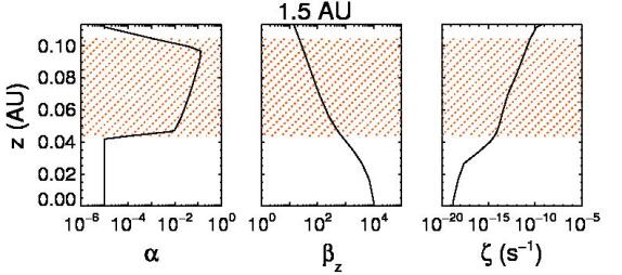
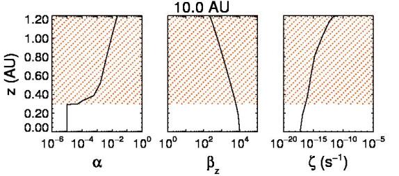
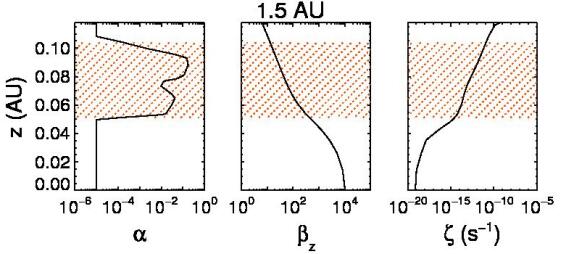
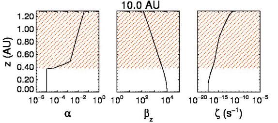
Figure 1.— Plots showing the multi-layered structure of evolved, magnetically active disks. Besides the dead zone and the active layer, both disks have a corona near the star and at the surface where the magnetic field is too strong for the tenuous gas to create turbulence. Disks may also have a double-layered active zone with a dead slice in some locations. Top left: $\alpha(z)$, $\beta_{z}(z)$ and $\zeta(z)$ of Model 1 at 1.5 AU after 1 Myr. Top right: Model 1 at 10 AU. Bottom left: Model 2 at 1.5 AU, 1 Myr. Bottom right: Model 2 at 10 AU. In each panel, the active region with $\Lambda>1$ and $\beta>\beta_{min}$ is shaded with red dots.

After the ionization rate is determined at each $(R,z)$ zone in our disk model, an interpolation through the look-up table can return the magnetic diffusivities. We can then compute the Elsasser number $\Lambda$ and $Am$ and determine whether MRI turbulence in the zone is active or not, according to our turbulence criterion (Section 2.1). The last remaining ingredient in our MRI prescription is a rule for determining the strength of the turbulence, where it is present. Where MRI is saturated, we use the scaling relations

$$\alpha =\frac{1}{2\beta}$$ (30)

$$\nu =\alpha c_{s}H=\frac{B^{2}}{16\pi\rho\Omega}$$ (31)

found between turbulent stress and magnetic field strength in a variety of shearing-box simulations (Hawley et al., 1995; Sano et al., 2004; Bai & Stone, 2011). Note that Equation 31 applies no matter the field geometry or value of $\Lambda$ or $Am$.

Since there is an accretion flow caused by large-scale magnetic fields even in the dead zone (Turner & Sano, 2008; Nelson & Gressel, 2010), we set a minimum value of $\alpha$ where the MRI is damped. In the active layer, $\alpha$ is close to its maximum value of $\sim 0.5$, set by the cessation of MRI in the strong-field limit of $\beta\geq 1$ (Hawley et al., 1995; Balbus & Hawley, 1998). Bai & Stone (2011) found a similar result in the ambipolar regime, $\alpha\approx 0.4$ for $Am\rightarrow\infty$. The shear stress in the dead zone is an order of magnitude less than in the active layer (Fleming & Stone, 2003; Turner et al., 2007; Turner & Sano, 2008), and the plasma $\beta$ at the midplane is typically two to three orders of magnitude higher than at the top of our grid (see Figure 1, which shows profiles of the vertical component of $\beta$, $\beta_{z}=8\pi P/B_{z}^{2}$, for two different disk radii). $\alpha_{min}$ must be therefore be roughly four orders of magnitude less than $\alpha_{max}$ to produce an appropriate level of dead zone shear stress. We take $\alpha_{min}=10^{-5}$ (Table 1).

3. Disk Structure and Mass Transport

With our method of computing turbulent viscosity at any location in a protostellar disk, we may now simulate how the disk re-distributes its mass throughout its multi-million-year existence. Since our viscosity prescription depends on the four inputs $T$, $\rho$, $\beta$ and $\zeta$, which are functions of radius and vertical height $(R,z)$, we must compute the detailed vertical and radial structure of the disk. Our computational setup, similar to the disk models of Dodson-Robinson et al. (2009), is based on the following simplifying assumptions:

1. The disk is axisymmetric and symmetric about the midplane;

2. The disk is geometrically thin, $H/R\ll 1$;

3. Heat escapes in the vertical direction much faster than it is carried with the gas flow in the radial direction.

Assumption 1 reduces the physical three-dimensional disk to a two-dimensional quadrant with zero flux at the midplane (required for symmetry). Neglecting the azimuthal dimension is a critical step in speeding up the code to allow long-timescale simulations. Assumption 2 allows the vertical and radial dimensions to be decoupled in a 1+1-D framework, so that energy transport proceeds only in the vertical direction. Each radial gridpoint contains an independent vertical structure model. Assumption 2 is valid as long as the vertical sound-crossing time (of order the orbital timescale) is much less than the accretion timescale, which is generally true in T-Tauri disks.

In section 3.1 we describe our vertical structure model, while in Section 3.2 we discuss our mass transport parametrization. Section 3.3 contains a description of our computational methods.

3.1. Vertical structure

Hydrostatic equilibrium and the thermal balance between stellar irradiation, radiative cooling and viscous heating govern the vertical structure of our disk. We use the flux-limited diffusion approximation for the transport of viscously generated energy. The accretion flux gradient is determined by the viscous energy generation rate per unit volume (Pringle, 1981):

$$\frac{\partial F_{acc}}{\partial z}=\frac{9}{4}\nu\Omega^{2}\rho.$$ (32)

In Equation 32, $\Omega$ is the height-dependent Keplerian frequency

$$\Omega=\left[\frac{GM_{*}}{\left(R^{2}+z^{2}\right)^{3/2}}\right]^{1/2}.$$ (33)

Temperature and pressure are related by the ideal gas equation of state,

$$P=\left(\frac{R_{g}}{\mu}\right)\rho T,$$ (34)

where $\mu=2.33$ g mol^-1 is the mean molar weight of the disk gas (Table 1). The temperature and pressure gradients are

$$\frac{\partial T_{acc}}{\partial z}=\frac{\partial P}{\partial z}\nabla\frac{T}{P},$$ (35)

$$\frac{\partial P}{\partial z}=-\rho\Omega^{2}z,$$ (36)

In Equation 35, $T_{acc}$ is the temperature contribution from viscous heating only—stellar irradiation and the ambient molecular cloud also contribute some of the thermal energy. $T$ is the true temperature and includes all heat sources.

To calculate $\nabla\equiv d\ln T/d\ln P$, the thermodynamic gradient, we use the Schwarzschild criterion for stability against convection:

$$\nabla=\left\{\begin{array}[]{l}\nabla_{rad},\nabla_{rad}\leq\nabla_{ad}\\ \nabla_{conv},\nabla_{rad}>\nabla_{ad}\end{array}\right..$$ (37)

$\nabla_{ad}=2/7$ is the adiabatic thermodynamic gradient for diatomic gas and

$$\nabla_{rad}=\frac{3}{4}\frac{\kappa PF}{ac\Omega^{2}zT^{4}},$$ (38)

is the radiative thermodynamic gradient, where $a$ is the radiation density constant and $\kappa$ is the local Rosseland mean opacity. For full details on how to compute $\nabla_{conv}$ in the disk’s convective zone, see Kippenhahn & Weigert (1994). Computing $\nabla$ requires the local Rosseland mean opacity, $\kappa$. At low temperatures, $T<700$ K, we use the opacities of Semenov et al. (2003) calculated for a 5-layered sphere topology. At higher temperatures where molecular gas dominates opacity ($T>1000$ K), we use the tables of Ferguson et al. (2005). For $700\;{\rm K}\leq T\leq 1000$ K, we interpolate between the two tables using a weighted average in $\log(T)$ space. For more details, and plots of the resulting opacities, see Dodson-Robinson et al. (2009).

Integrating the coupled ODEs in Equations 32, 35 and 36 requires two different temperatures: $T$, the true temperature resulting from all sources of thermal energy, and $T_{acc}$, the component from viscous heating only. The other heat sources are the central star, which sets an equilibrium temperature component $T_{eq}$, and the ambient star-forming region, from which long-wavelength radiation that penetrates the disk sets a minimum temperature $T_{amb}$. To compute $T_{eq}$, we begin by assuming the disk surface is flared as a result of hydrostatic equilibrium and radiative equilibrium with the star. Following the models developed by Chiang & Goldreich (1997), we calculate the grazing angle $\theta$ at which stellar energy enters the disk:

$$\theta\approx\frac{8}{7}\left(\frac{T_{*}}{T_{c}}\right)^{4/7}\left(\frac{R}{R_{*}}\right)^{2/7},$$ (39)

where $R_{*}$ and $T_{*}$ are the star’s radius and effective temperature and $T_{c}$ is a measure of the gravitational potential at the surface of the star:

$$T_{c}=\frac{GM_{*}\mu}{\sigma R_{*}}.$$ (40)

In Equation 40, $M_{*}$ is the star’s mass and $\sigma$ is the Stefan-Boltzmann constant. As the disk evolves, we determine the star’s temperature and radius as a function of age from the pre main-sequence evolutionary tracks of D’Antona & Mazzitelli (1994). Since the star’s luminosity decreases as it moves down the Hayashi track, the disk flaring becomes less pronounced over time and the disk surface, where $T\approx T_{eq}$, cools.

In the direction parallel to the disk midplane, the stellar radiation penetrates to an optical depth $\tau_{*}^{\|}\sim 1$. The asterisk subscript denotes that this optical depth is measured at the peak wavelength of the starlight, near $1\;\mu$m. Measured perpendicular to the disk midplane, stellar radiation is mostly attenuated by optical depth $\tau_{*}^{\bot}\sim\tau_{*}^{\|}\theta\sim\theta$. The equilibrium temperature between the stellar heating and radiative cooling at the disk surface—neglecting viscous heating—is (D’Alessio et al., 2006; Natta et al., 2000):

$$T_{eq,surf}\approx 0.8\left(\frac{\theta}{\tau_{surf}}\right)^{1/4}\left(\frac{R_{*}}{R}\right)^{1/2}T_{*},$$ (41)

where $\tau_{surf}$ is the Rosseland mean optical depth at the disk surface for blackbody radiation at $T_{eq,surf}$. The top surface of our vertical grid is defined by $\tau_{surf}=0.2$. Since half of the stellar radiation absorbed by grains at the disk surface is re-radiated into space, the equilibrium temperature with the star as a function of height in the disk—again, neglecting viscous heating—is

$$T_{eq}(z)^{4}=\frac{1}{2}T_{eq,surf}^{4}e^{-\tau_{z}},$$ (42)

where $\tau_{z}$ is the Rosseland mean optical depth to height z:

$$\tau_{z}=\int_{z}^{z_{surf}}\kappa\rho\>dz.$$ (43)

Finally, the true temperature $T$ simply the flux sum of the individual temperature components:

$$T^{4}=T_{acc}^{4}+T_{eq}^{4}+T_{amb}^{4}.$$ (44)

3.2. Radial diffusion

Since the radial and vertical dimensions of our disk model are decoupled, we must treat mass transport as a one-dimensional problem. Yet the MRI-active, partially ionized disk is vertically layered, with the most active accretion occurring at the surface. The key to a successful 1-D description of layered accretion is the fact that vertical re-distribution of mass within an annulus occurs more quickly than accretion in the active layers: $1/\Omega\ll R^{2}/\nu_{active}$. By computing a mass-weighted, vertically averaged value of turbulent viscosity in each annulus,

$$\bar{\nu}=\frac{2}{\Sigma}\int_{z=0}^{z_{surf}}\nu\rho dz,$$ (45)

where $\Sigma$ is the surface density in the annulus, we can describe mass transport using the radial diffusion equation:

$$\frac{\partial\Sigma}{\partial t}=\frac{3}{R}\frac{\partial}{\partial R}\left[R^{1/2}\frac{\partial}{\partial R}\left(\Sigma\bar{\nu}R^{1/2}\right)\right].$$ (46)

In each $(R,z)$ zone, we compute viscosity according to Equation 1. We use a height-dependent modified scale height $H$,

$$H=\frac{c_{s}/\Omega}{\sqrt{1+\left(2z^{2}\Omega^{2}/c_{s}^{2}\right)}},$$ (47)

softened into a non-singular form (Milsom et al., 1994). In MRI-active zones, $\alpha$ is given by Equation 31, while in inactive zones we set $\alpha$ to our chosen value of $\alpha_{min}$ (Table 1). The sound speed used to compute $\nu(R,z)$ is

$$c_{s}^{2}=\frac{R_{g}}{\mu}T.$$ (48)

3.3. Computational methods and initial conditions

To initialize the disk evolution model, we compute the vertical structure of a disk with the following features:

1. A surface density profile $\Sigma\propto R^{-3/2}$, predicted by Zhu et al. (2010) for layered accretion disks in the T-Tauri phase.

2. A pre-main-sequence star with a mass of 0.95 $M_{\sun}$ and an initial age of 0.1 Myr, which roughly coincides with the beginning of the T-Tauri phase (Dunham & Vorobyov, 2012). The star will continue to accrete a small amount of mass from the disk during the $\sim 3$ Myr T-Tauri phase.

3. An ambient temperature of 20 K (Table 1) to match the typical background temperatures of infrared dark clouds (Peretto et al., 2010).

4. An outer radius of 70 AU, set by the 80 AU solar nebula size limit of Kretke et al. (2012). (Note that the disk expands from its initial radius.) Kretke et al. show that a solar nebula with $R_{out}>80$ AU would excite Kozai oscillations in some of the planetesimals scattered by Jupiter and Saturn, stranding them in stable, high-inclination, low-eccentricity orbits that surveys have not detected.

5. An inner radius of $R_{in}=0.5$ AU. The requirement that the disk stay below the dissociation temperature of H₂, so that the ideal gas equation holds, dictates our choice of $R_{in}$. Ruden & Lin (1986) find that the exact value of $R_{in}$ does not affect the overall disk structure as long as $R_{out}\gg R_{in}$.

6. A disk mass of either $0.015M_{\odot}$ (Model 1) or $0.03M_{\odot}$ (Model 2). Our disk masses are designed to be comparable to previous global-disk MRI simulations (e.g. Lyra et al., 2008; Dzyurkevich et al., 2010; Bai, 2011), almost all of which use minimum-mass solar nebulae. Note that such low-mass disks are probably not viable giant planet-forming environments (e.g. Thommes et al., 2008). In a forthcoming study, we will examine the evolution of MRI-active, high-mass, planet-forming disks.

We then evolve the disk forward in time using Equation 46. We use fully implicit finite differencing, adjusting the timestep $\Delta t$ so that surface density varies by a maximum of 1.0% during a single timstep. The inner boundary $R_{in}$ experiences zero stress, such that matter falls directly from $R_{in}$ onto the star. The disk is allowed to expand freely from the outer boundary $R_{out}$, with four new zones added to the disk each diffusion time of $R_{out}^{2}/\bar{\nu}(R_{out})$.

At each timestep, we independently calculate the vertical structure for each zone in the radial grid. We begin the vertical structure solver with initial guesses of $T_{acc}$, $\rho$ and vertical component of the magnetic pressure $P_{B,z}=B_{z}^{2}/8\pi$ at the top of our grid, defined by $\tau_{surf}=0.2$. We find the height of the grid surface by

$$z_{surf}=\frac{\kappa(\rho,T)P}{\Omega^{2}\tau_{surf}}$$ (49)

The accretion flux at the grid surface is $F_{acc}(z_{surf})=\sigma T_{acc}^{4}$. We use a fourth-order Runge-Kutta integrator with adaptive stepsize control to integrate the coupled ODEs in Equations 32, 35 and 36 from the surface to the midplane. The vertical magnetic pressure stays constant in height, though it varies with radius. A solved vertical structure model has the properties

$$F_{acc}(z=0)=0,$$ (50)

required to keep the disk symmetric about the midplane,

$$2\int^{z_{surf}}_{z=0}\rho dz=\Sigma,$$ (51)

so that the volume densities add up to the surface density in the annulus, and

$$\beta(z=0)=1000.$$ (52)

Equation 52 requires that the plasma $\beta$ be constant throughout the disk midplane. After turbulence is established, Fromang & Nelson (2006) find midplane values of $100\lesssim\beta\lesssim 1000$ for a wide range of vertical box sizes, resolutions and boundary conditions in global ideal MHD calculations. We use the Newton-Raphson algorithm (Press et al., 1992) to adjust the initial guesses of $T_{acc}$, $\rho$ and $P_{B,z}$ until a solution is found that satisfies Equations 50, 51, and 52.

The on-off nature of the MRI creates discontinuities in and $\nu(z)$ and $F_{acc}(z)$ that can cause the Newton-Raphson algorithm to oscillate between two sets of input parameters that bracket the correct solution of Equations 50, 51 and 52. To avoid such oscillations in the Ohmic regime, we decrease the value of $\alpha$ gradually in the range $1.6\geq\Lambda\geq 0.4$, using a sigmoid function:

$$\alpha\rightarrow\alpha/(1+e^{-k(\Lambda-1)}),$$ (53)

where $k=1.5\ln(1/(\alpha_{min}\beta)-1)$. We use a similar sigmoid function to smooth $\alpha$ in the ambipolar regime for $0.4\beta_{min}\leq\beta\leq 1.6\beta_{min}$.

4. Mass Transport in MRI-Active Disks

Here we present our simulations of the evolution of magnetically turbulent disks over million-year timescales. In §4.1, we discuss the relative sizes of the dead zone and active layers (Question 1 in Introduction). In §4.2, we demonstrate how the shrinking of the active layer over regions of high density enhances mass pileup in the dead zone. We also analyze the radial mass flow $\dot{M}(R)$ through the disk and show that the disk never reaches a steady state, even on million-year timescales (Question 2 in Introduction). In §4.3, we give a simple prescription for accretional heating due to MRI for use with semi-analytical, non-evolving disk models to predict observables (Question 3 in Introduction).

4.1. Turbulent Structure

Figure 2 shows viscosity as a function of $(R,z)$ for the inner 30 AU of Model 1 ($0.015M_{\odot}$, top) and Model 2 ($0.03M_{\odot}$, bottom). Outside of 30 AU, viscosity is almost independent of height $z$. The left-hand panels of Figure 2 show the disks after $10^{4}$ years of simulation time—a star age of 0.11 Myr, since we began the simulations with a star at the beginning of the T-Tauri phase, age 0.1 Myr (Dunham & Vorobyov, 2012). The right-hand panels show both model disks after 1 Myr of simulation time. The plots reveal two important features of the evolution of low-mass, MRI-active disks:

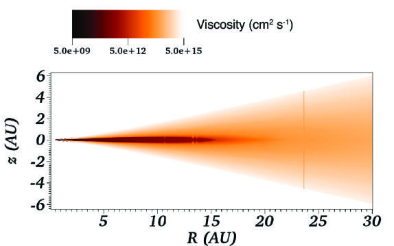
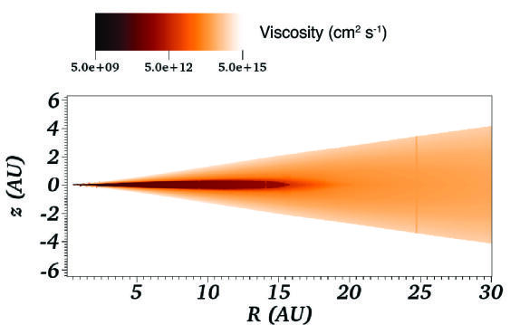
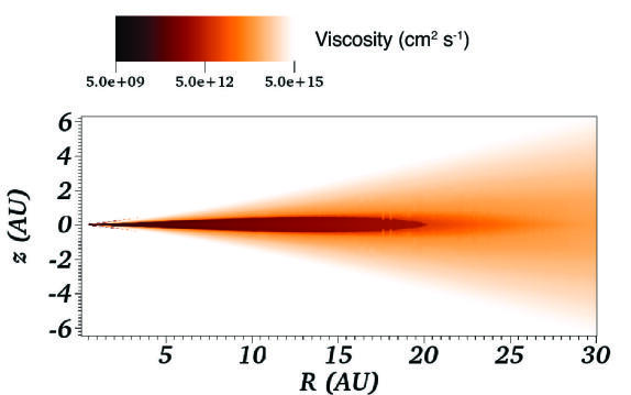
Figure 2.— Viscosity as a function of $(R,z)$ at two timepoints during disk evolution. The more massive Model 2 disk has the larger dead zone, which extends past 20 AU. In both models, the radial extent of the dead zone stays approximately constant with time. Top left: Model 1 (disk mass $0.015M_{\odot}$), $10^{4}$ years of simulation time (star age 0.11 Myr). Top right: Model 1 after 1 Myr of simulation time. Bottom left: Model 2 after $10^{4}$ years of simulation time. Bottom right: Model 2 after 1 Myr of simulation time.

1. A midplane dead zone, where Ohmic diffusion quenches the MRI and restricts viscosity, extends to 16 AU in Model 1 and 21 AU in Model 2.

2. Although the vertical heights of both the dead zone and the overall disk shrink with time as the disk loses mass and cools (see Section 5), the radial extent of the dead zone stays approximately constant in time.

The radial size of the dead zone is larger than the $\sim 5$ AU typically quoted for disks similar to the minimum-mass solar nebula (MMSN) (Matsumura & Pudritz, 2003; Salmeron & Wardle, 2008; Flaig et al., 2012). Here we define the dead zone as the region of the disk where $\Lambda<1$. The primary reason our dead zone is so extensive is the surface density of our disks: the MMSN contains $0.01M_{\odot}$ within 100 AU of the sun, while our least massive disk contains $0.015M_{\odot}$ within 70 AU. Our dead zone is also extensive because we treat ambipolar diffusion, as well as Ohmic diffusion. Sano et al. (2000) use the same tenfold dust depletion we do, but treat only Ohmic diffusion and find a dead zone that extends 5–10 AU.

Dead zones with $\alpha\simeq 10^{-5}$ are required for maintaining compositional gradients such as the ice gradient in the asteroid belt, which would radially diffuse on million-year timescales for fully turbulent disks (Nelson & Gressel, 2010). The fact that Uranus and Neptune have atmospheres with higher carbon enrichment than Jupiter and Saturn provides some evidence that the solar nebula had compositional gradients covering the entire giant planet-formation region (Encrenaz, 2005). Given that the dead zone in a disk of just $0.015M_{\odot}$ can reach $\sim 15$ AU, the outer boundary of the giant planet-formation region in the Nice model (Tsiganis et al., 2005), the solar nebula could have supported such a compositional gradient. The lack of change in the dead zone radius over time suggests that compositional gradients are stable over million-year timescales.

Figure 1 gives further insight into the vertical structures of Model 1 (top) and Model 2 (bottom). In each panel, the active layer is shaded with red dots. At 10 AU, both disks show the classical layered structure of an MRI-active zone on tope of a dead zone. At 1.5 AU, however, we see additional complexity in the disk’s vertical structure. At 45 mG (Model 1) and 70 mG (Model 2), the magnetic tension is strong enough to prevent MRI from bending the field lines in the low-density surface gas despite a high ionization rate of $10^{-10}$ s^-1, forming a stable corona (e.g. Miller & Stone, 2000). Our stabilizing magnetic field values are roughly consistent with those of Salmeron & Wardle (2008), who calculated that unstable MRI modes can only grow for $B\lesssim 80$ mG in the presence of $1\mu m$ grains. (See §2.2 and Table 1 for more on the grain properties used in our models.) Figure 3 is a zoom-in on the stress coefficient $\alpha(R,z)$, viscosity $\nu(R,z)$ and ionization rate $\zeta(R,z)$ in the inner 4 AU of Model 2 after 1 Myr. The inactive corona is apparent for radii $R\lesssim 3$ AU, but moves above our computed disk surface (the location where $\tau_{*}^{\|}\sim 1$) as the magnetic field stength decreases with radius.

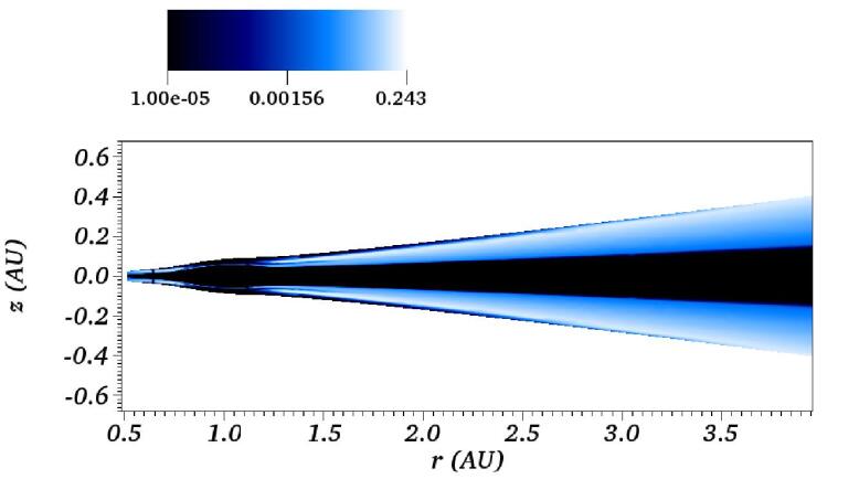
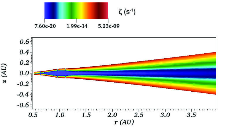
Figure 3.— Plots of viscosity $\nu$ (top), turbulent stress coefficient $\alpha$ (middle), and ionization rate $\zeta$ (bottom) for the inner 4 AU of Model 2 at 1 Myr. In the inner 3 AU, a stable corona where ambipolar diffusion shuts down MRI sits on top of the active layer. Note the thinness of the active layer over the pileup at 1 AU. The dead slice seen in Figure 1 is also visible between 1.2 AU and 1.7 AU.

Also noticeable in Figures 1 and 3 is a split active layer in the inner part of Model 2. MRI-active regions of high $\alpha$ and $\nu$ sandwich a “dead slice” that has reduced stress and viscosity by an order of magnitude. (The fact that $\alpha$ does not immediately plunge to its minimum value in the dead slice is a result of the sigmoid smoothing described in §3.3.) While not present at the start of our simulations, the split active layer appears after only 5000 years of disk evolution and persists until the end of the simulation at 3 Myr. The split active layer extends from roughly $1.2$ AU $<R<1.7$ AU (Figure 3), though its radial extent shrinks slightly as the disk evolves.

The dead slice, in the part of the disk where ambipolar diffusion is the strongest non-ideal MHD term, is the result of two competing effects. First, MRI in the ambipolar regime requires high ionization: decreasing $\zeta$ toward the disk midplane reduces $Am$ and shuts down turbulence. Yet ambipolar diffusion is quenched at high densities: increasing $\rho$ toward the midplane increases $Am$, favoring turbulence. In the dead slice, the dropping $\zeta$ temporarily dominates over the increasing $\rho$ and shuts down the MRI. Model 1 does not have a dead slice because its surface density is about 1/2 that of Model 2: $\zeta$ can stay high enough for the MRI to operate until very near the midplane, where Ohmic diffusion begins to dominate. An open question is whether or not a dead slice would be present in a fully 3-D simulation with identical vertical profiles of $\rho$, $\zeta$ and $\beta$ to our disk: the thickness of the dead slice is smaller than the MRI wavelength by a factor of 2–10, so turbulence would very likely erase it.

We have seen that MRI-active disks may have complex vertical structure, with multiple layers of turbulent and non-turbulent zones. In the next section we explore the overall mass flow through the disk and discuss its evolution on million-year timescales.

4.2. Mass Flow

As might be expected for a layered disk with a dead zone, radial mass transport is not in steady state for either Model 1 or Model 2. The left-hand panel of Figure 4 shows

$$\dot{M}(R)=2\pi R\Sigma v_{R}$$ (54)

for both models after 1 Myr of evolution, where $v_{R}$ is a density-weighted, vertically averaged gas radial velocity. The convention in Equation 54 is that $v_{R}$ is positive when gas flows toward the star and negative when gas flows away from the star. In the inner part of the disk, where gas flows inward, the highest accretion rates occur (a) at the outer edge of the dead zone (at 21 AU for Model 1 and 16 AU for Model 2), and (b) at the inner disk boundary. There is a clear drop in $\dot{M}(R)$ associated with the dead zone. (The noisy $\dot{M}$ profile where the disk has two or more layers is a reflection of the root-finding tolerance in our Newton-Raphson algorithm. Fluctuations in the location of the boundary between dead and active zones are random and average out over time.)

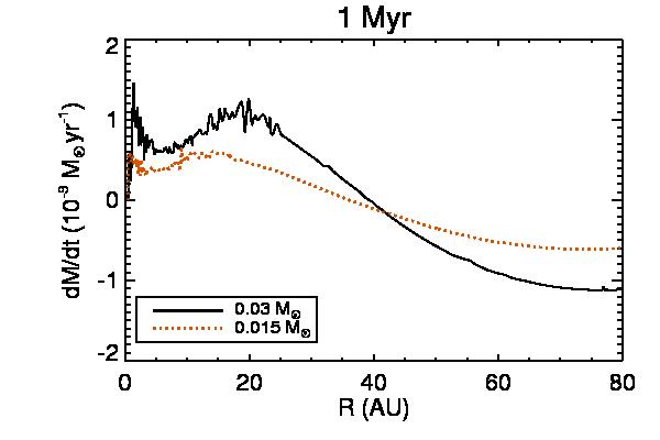
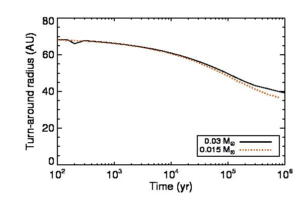
Figure 4.— Left: A plot of $\dot{M}(R)$ for both disk models after 1 Myr of disk evolution reveals that low-mass MRI-driven accretion disks have not reached steady state after 1 Myr. As required by conservation of angular momentum, there is a turn-around in the mass flow between inward accretion and outward decretion. The highest accretion rates in the inner disk, where mass moves toward the star, occur on either side of the dead zone. Right: The location of the turn-around radius as a function of time for both models. The turn-around radius moves inward over time.

The potential for the dead zone to become gravitationally unstable, given enough time to accumulate mass, is clear (Gammie, 1996; Armitage et al., 2001; Zhu et al., 2010)—though we see only a slow, steady density growth at $\sim 1$ AU–4 AU over the course of 3 Myr in Model 2 (Figure 5). We will examine the potential for gravitational instability in high-mass, MRI-active disks in a forthcoming paper. One important caveat is that the accumulation of mass in the dead zone is unstable to the Rossby wave instability (Hawley, 1987; Li et al., 2001; Meheut et al., 2012), which triggers spiral density waves. Without azimuthal information in our model, we cannot model the effect of the Rossby wave instability on dead-zone overdensity. Ultimately, the overdensity may not survive and may break up into large-scale vortices (Papaloizou & Pringle, 1985; Lovelace et al., 1999).

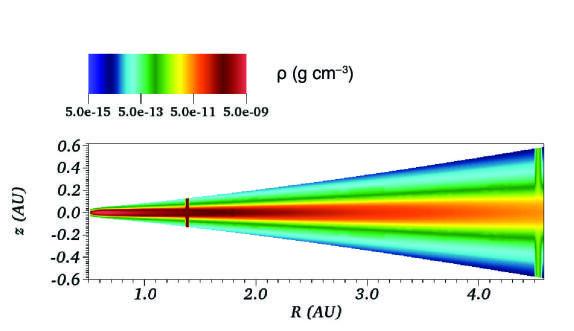
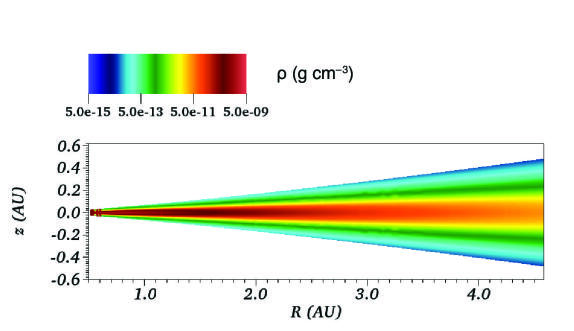
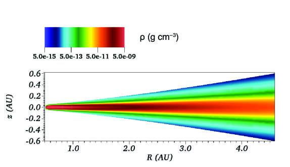
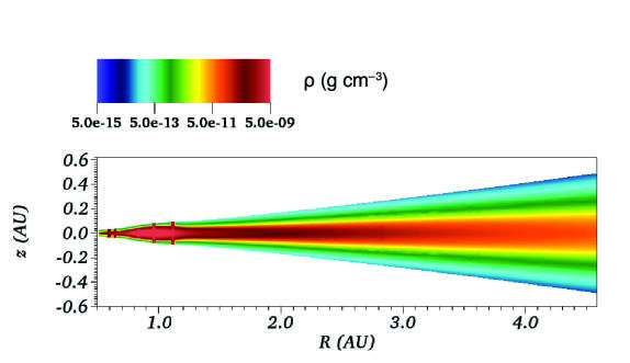
Figure 5.— Volume density as a function of $(R,z)$ at two timepoints during disk evolution. In the more massive Model 2, the density in the pileup at 1 AU noticeably grows with time. Top left: Model 1 (disk mass $0.015M_{\odot}$), $10^{4}$ years of simulation time (star age 0.11 Myr). Top right: Model 1 after 1 Myr of simulation time. Bottom left: Model 2 after $10^{4}$ years of simulation time. Bottom right: Model 2 after 1 Myr of simulation time.

At $t=1$ Myr, there is turn-around in the accretion flow near 40 AU in each model. The outward mass flow outside 40 AU is necessary for overall conservation of angular momentum as material in the inner disk moves toward the star. The fact that there must be a change in the accretion flow direction also follows directly from the diffusive nature of T-Tauri disks (e.g. Lynden-Bell & Pringle, 1974), which lack a circumstellar envelope to feed steady-state inward accretion. In both models, the disk has expanded beyond its initial 70 AU size after 1 Myr. Note that the 40 AU region of the disk does not drain, as the “turn-around radius” where the accretion flow changes direction moves inward with time (right-hand panel of Figure 4). We heartily discourage the use of a steady-state accretion rate for any reasonable description of angular momentum transport in T-Tauri disks. However, for predicting observables to order-of-magnitude using a static, non-time-varying disk model, we suggest approximating the accretional heating in MRI-active disks with a constant $\dot{M}\sim 10^{-9}M_{\odot}$ yr^-1. Figure 4 suggests that at a given time, $\dot{M}$ has a modest dependence on disk mass.

How consistent are our modeled accretion rates with observations? An oft-quoted value of $\dot{M}_{*}$, the T-Tauri star accretion rate, is $10^{-8}M_{\odot}$ yr^-1 (Sicilia-Aguilar et al., 2004). Accretion rates in transitional disks are roughly $3\times 10^{-9}M_{\odot}$ yr^-1 (Espaillat et al., 2012). Our simulations achieve an accretion rate of roughly $\dot{M}_{*}\sim 10^{-9}M_{\odot}$ yr^-1, more consistent with the median transitional disk accretion rate. Reproducing high accretion rates in the inner regions of MRI-active disks is a delicate balance between magnetic field strength, X-ray ionization, grain size, and gas/small grain mass ratio. For example, we performed simulations using the same disk masses and X-ray luminosity (0.015$M_{\odot}$ and 0.03 $M_{\odot}$; $2\times 10^{30}$ erg s^-1, respectively) but a grain size of $0.1\mu$m instead of $1\mu$m and a standard gas/small grain mass ratio of 100, and quenched all MRI activity in the disk entirely. However, as models by Zsom et al. (2011) show grain growth and settling within 1000 years, it is reasonable to assume the gas/small grain mass ratio has evolved from the interstellar value by the T-Tauri phase. In our simulations, a stronger magnetic field (lower value of $\beta$ at the midplane) also suppressed MRI-driven accretion, which occurs in regions of the disk dominated by ambipolar diffusion. Most simulations of non-ideal MRI-driven accretion have difficulty reaching the $10^{-8}M_{\odot}$ yr^-1 benchmark (e.g. Zhu et al., 2010; Bai, 2011), though there is a substantial amount of scatter in both T-Tauri and transitional disk accretion rates (Romero et al., 2012).

4.3. Simple prescription for accretional heating in an MRI-active disk

Previous studies have often relied on static, non-evolving disk models to connect measured line fluxes, velocities or spectral indices to physical properties of disks (e.g. D’Alessio et al., 2006; Pinte et al., 2010). Unfortunately the constant-$\alpha$ prescription for turbulent angular momentum transport leads to unphysical thermodynamic descriptions of disk midplanes. Predicted midplane temperatures in a constant-$\alpha$ model, where most turbulence is concentrated at the midplane, are too high. The poor match of the constant-$\alpha$ model to realistic protostellar disk accretion is definitely a problem for observations that trace disk midplanes, such as sub-millimeter measurements of continuum emission from large grains or surveys of rare molecules like HCO⁺ or HD. However, the problem also affects observations that trace surface layers, such as Spitzer emission lines, infrared SEDs and sub-millimeter maps of abundant gases like CO. If a significant subset of T-Tauri disks rely on MRI to drive accretion, overestimating their midplane temperatures leads to overpredicting the photosphere and pressure scale heights, underpredicting the optical depths of low-excitation lines such as CO ($J=2\rightarrow 1$), and possibly underpredicting the rates of grain settling and growth.

Here we use our simulation results to present a simple prescription for $\alpha$ in an MRI-active disk. First we determine the depth of the MRI-active layer. Figure 6 shows the surface density of the active layer as a function of radius for four time snapshots of Model 1 (left) and Model 2 (right). Clearly, the functional form of $\Sigma_{\rm active}(R)$ is the same for both models and does not vary significantly with time. Near the star, where X-ray ionization is important, $\Sigma_{\rm active}$ is high but falls off quickly as X-ray irradiation declines (see Equation 29). Over the dead zone, in the region where only cosmic-ray ionization is important, $\Sigma_{\rm active}(R)$ increases as the magnetic field weakens, shrinking the inactive corona. $\Sigma_{\rm active}(R)$ reaches its maximum at the outer edge of the dead zone. Here, where the entire vertical column is active, the decreasing depth of the active layer simply reflects the fact that $\Sigma(R)$ is a decreasing function.

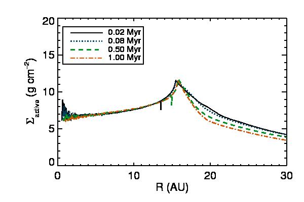
Figure 6.— $\Sigma_{\rm active}(R)$ for four time snapshots of Model 1 (left) and Model 2 (right). The active column depth as a function of radius changes very little as the disk evolves, making it possible to approximate $\Sigma_{\rm active}(R)$ for use in a semi-analytical viscosity prescription.

Although $\Sigma_{\rm active}$ does vary with $R$ in the parts of the disk with a dead zone, the variation is less than a factor of two for both models presented here. Similarly, $\Sigma_{\rm active}(R)$ is slightly higher for Model 2 than for Model 1, suggesting that the active column may increase modestly with disk mass. $\Sigma_{\rm active}\approx 10$ g cm^-2 is a good approximation for low-mass disks with surface density less than about four times the MMSN. The semi-analytical viscosity prescription is then simple:

1. Set the depth of the active column to $\Sigma_{\rm active}\approx 10$ g cm^-2. Set $\alpha\approx 0.01$ in the active column and $\alpha\approx 10^{-5}$ in the dead zone. While there may be a corona on the inner disk surface, it contains very little mass and may safely be ignored as long as the disk model includes stellar heating.

2. Smooth the transition between the active layer and the dead zone if desired.

3. The entire vertical column will be active where $\Sigma\approx 20$ g cm^-2, such that the two active layers meet at the midplane. Outside the outer radius of the dead zone, where $\Sigma\approx 20$ g cm^-2, use $\alpha\approx 0.01$.

4. Calculate viscosity $\nu$ at each $(R,z)$ in the disk using Equation 1.

5. Thermal Evolution of MRI-Active Disks

Now that we understand how mass moves through a disk where accretion is driven by MRI, we turn our attention to the thermal structure and evolution of the disk. Here we see some important differences from disk models that use a constant-$\alpha$ viscosity prescription. In Section 5.1 we discuss how different parts of MRI-active disks heat up and cool off over time (Question 4 in Introduction). In Section 5.2 we investigate the location of the ice line and its motion through an MRI-active disk (Question 5 in Introduction).

5.1. Disk Heating and Cooling

The top panels of Figure 7 show the surface and midplane temperatures of Models 1 and 2 after 10 thousand years of evolution (left) and 1 Myr of evolution (right). First, note the obvious feature that the surface is far hotter than the midplane throughout most of the disk. Disk models with constant-$\alpha$ viscosity prescriptions usually have warm midplanes, $T\gtrsim 100$ K, in the inner 5 AU. In the inner 1 AU of constant-$\alpha$ models, the midplane temperature can even exceed the surface temperature, approaching 1000 K (e.g. Hersant et al., 2001; D’Alessio et al., 2006; Dodson-Robinson et al., 2009). In our models, there is so little turbulent energy generated in the dead zone that the disk midplane falls to 20 K—the ambient temperature of the remnant molecular cloud surrounding the disk. Here we assume the disk is optically thin to long-wavelength radiation from the ambient cloud and cannot cool below the ambient temperature. Only in the inner $\sim 2$ AU does residual mass transfer by large-scale magnetic fields lift the midplane temperature above the minimum value.

Figure 7.— Although the surface of the disk cools over time, as the T-Tauri star moves down the Hayashi trach, parts of the midplane of an MRI-active disk may heat up over time as mass piles up in the dead zone. Top left: Temperature at the surface (top curves) and the midplane (bottom curves) of Model 1 (red dotted) and Model 2 (black solid) after 10,000 yr. Top right: Surface and midplane temperatures of Models 1 and 2 after 1 Myr. Note the increase in midplane temperature at the edge of the dead zone in each model. Bottom left: Contour plot of $T(R,z)$ in the inner 4 AU of Model 2 after 10,000 yr of evolution. Temperature units are Kelvins. Bottom right: Contour plot of $T(R,z)$ in the inner 4 AU of Model 2 after 1 Myr of evolution. Note how the pileup of material centered at 1 AU (see Figure 5) has heated up over time.

Moving outward through the disk, the midplane temperature rises modestly until it equalizes with the surface temperature where the disk becomes optically thin to stellar radiation. Both of our models, despite their modest masses ($0.015M_{\odot}$ and $0.03M_{\odot}$), are optically thick to stellar radiation inside $\sim 70$ AU, decoupling the surface and midplane temperatures. Passively heated disk models (e.g. Woitke et al., 2009) are therefore poor approximations to the midplane temperatures of our model disks, as are constant-$\alpha$ models in which $T$ decreases with $R$ at the midplane. Instead, coupling the simple viscosity prescription in Section 4.3 with a radiative transfer scheme is preferable for modeling observables that trace the inner $\sim 70$ AU.

Figure 7 shows that the disk surface cools off over time, as expected for any disk being irradiated by a T-Tauri star evolving along the Hayashi track. The surface cooling affects the disk structure as follows:

1. The overall photosphere height of the disk decreases with time (Equation 39; Figures 2, 5 and 7);

2. The viscosity in the surface layers decreases with time (Equation 31; Figure 2).

The decrease in surface viscosity with time is due to the increasing density in the surface layers as the disk cools.

Despite the fact that the disk surface cools with time, the tendency of the MRI to pile up mass unevenly leads the temperature to increase with time in certain parts of the disk. The bottom panels of Figure 7 show the temperature increase in the pileup at 1 AU in Model 2. Though modest, the temperature increase does affect the location of the ice line, which we discuss in the next section.

5.2. The Ice Line in MRI-Active Disks

Ice forms in protoplanetary disks when the temperature falls below 145-170 K, depending on the water vapor’s partial pressure (Podolak & Zucker, 2004; Lecar et al., 2006). Observations of the outer asteroid belt place the ice line in today’s Solar System at 2.7 AU. Theoretical estimates of the ice line location in the solar nebula place it a minimum of 0.6 AU from the sun (Davis, 2005; Garaud & Lin, 2007) and a maximum of 6 AU at the beginning of the T-Tauri phase, moving inward as the disk evolves (Dodson-Robinson et al., 2009). In constant-$\alpha$ disks, the ice line moves inward with time as the optically thick disk radiates away its accretion energy. At late times, however, the inner disk loses enough mass to become optically thin to stellar irradiation, causing the ice line to move outward with time (Garaud & Lin, 2007; Oka et al., 2011). The more massive a constant-$\alpha$ disk, the higher its midplane temperature will be. Taking the Davis (2005), Garaud & Lin (2007) and Oka et al. (2011) disk models up to a reasonable planet-forming mass of $0.04M_{\odot}$ or higher (Thommes et al., 2008) would push their ice lines outside the terrestrial planet-forming region, more in agreement with the results of Dodson-Robinson et al. (2009).

In an MRI-active disk, the overall thermal evolution is determined by the dimming of the parent star, which causes viscosity in the active surface layers to decrease with time (see Section 5.1). Figure 8 shows the 2-D structure of the ice line in Model 2 at timepoints 100 yr, 1000 yr, 10,000 yr, 100,000 yr, 1 Myr and 3 Myr. At early times, we recover the “two-branch” structure of the ice line seen by Davis (2005), in which a nearly horizontal ice line divides the hot surface from the cool interior and a midplane ice line separates the warm midplane near the star from the cool midplane far away from the star. After 10,000 yr of evolution, the inner edge of the disk at 0.5 AU cools enough for ice to freeze at the midplane, causing a “pinch-off” in the midplane branch of the ice line that leaves an H₂O gas bubble at 0.6 AU. This pinch-off is probably a boundary effect: since mass flows freely from our inner boundary at 0.5 AU onto the star, the disk near our inner boundary loses mass and cools quickly.

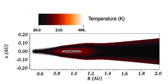
Figure 8.— In the inner 2 AU of Model 2, we see that the disk surface cooling and midplane heating both affect the structure of the ice line. Each plot shows $T(R,z)$ with the ice line at 160 K indicated by the blue contour (temperature units are Kelvins). Simulation times are 100 yr (top left), 1000 yr (middle left), 10,000 yr (bottom left), 100,000 yr (top right), 1 Myr (middle right) and 3 Myr (bottom right). Recall that the star age is already 0.1 Myr at the beginning of the simulation.

By 1 Myr, mass loss from the inner edge of our grid combined with less activity in the surface layers cools the disk enough to push the midplane ice line inside 0.5 AU, the inner boundary of our computation. Here our results are still consistent with the low-mass models of Davis (2005), Garaud & Lin (2007) and Oka et al. (2011), who all show the ice line moving inside 1 AU for accretion rates $\dot{M}\sim 10^{-10}M_{\odot}$ yr^-1. An important difference between our models and those of Davis (2005), Garaud & Lin (2007) and Oka et al. (2011) is that the accretion rate does not have to drop extremely low for the terrestrial planet-forming region to cool enough to freeze ice: both Model 1 and Model 2 have active layers that drive $\dot{M}\sim 10^{-9}M_{\odot}$ yr^-1 through the disk surface. Our model disks predict colder midplanes in the inner 10 AU than those of Terquem (2008) due to the lower minimum $\alpha$ assumed here ($\alpha_{min}=10^{-5}$ for our work vs. $\alpha_{D}=10^{-3}$ or $\alpha_{D}=10^{-4}$ in Figure 3 of Terquem (2008), where $\alpha_{D}$ the value of $\alpha$ in the dead zone). Unlike Terquem (2008), our disk has a colder midplane than surface because we include the effects of stellar heating.

The MRI can also create local regions that heat up with time not because the disk becomes optically thin, but because mass piles up in the dead zone. Between 1 Myr and 3 Myr of evolution, the pileup at 1 AU of Model 2 heats up enough for the midplane ice line to reappear—a real physical effect. Model 1, which does not show any such pileup, follows a similar evolutionary path as Model 2 up to 1 Myr. In an MRI-active disk, water ice in the terrestrial planet-forming region may be transient. Understanding which parts of the inner disk have water ice available for planet formation requires a careful comparison of the planetesimal growth timescale, the star cooling timescale and the growth timescale of any pileups deposited in the dead zone. In Model 2, the pileup grows and the star dims on a timescale similar to the disk lifetime. We will examine high-mass MRI-active disks, in which dead-zone pileups can grow much more quickly, in a forthcoming paper.

6. Model Limitations

Although our model incorporates much of the physics of disk evolution during the T-Tauri phases of stars, our long-timescale computation requires a number of simplifications. Our disk accretion model suffers from the following limitations, which may affect our conclusions:

1. We model our disks as 1+1d instead of 3d. We assume radial symmetry, and that the vertical structure is not coupled to the radial mass transport. This ignores the possibility of accretion driven by non-axisymmetric instabilities not represented by our parameterization of stress from MHD turbulence, such as the Rossby wave instability (Hawley, 1987; Li et al., 2001; Meheut et al., 2012). We may then underestimate accretion rates in some regions of the disk.

2. We do not model the effects of gravitational instability on momentum transport, as is done by Martin et al. (2012b), but instead limit our simulations to those disks which are gravitationally stable for their entire lifetime. To test whether a disk is gravitationally stable to axisymmetric perturbations, we calculate the Toomre Q parameter at every radial grid point. Stability requires that

   $$Q\equiv\frac{c_{s}\Omega}{\pi G\Sigma}>Q_{crit}\approx 1.$$ (55)

   Note that for disks more massive than those we have simulated, the disk does eventually become gravitationally unstable to axisymmetric perturbations within the dead zone (see Section 4.2).

3. We do not model the effects of Hall diffusivity, which is the least well understood magnetic diffusion regime. However, it is unlikely to alter either the conditions required for MRI or the strength of the turbulence where Ohmic dissipation is also present (Sano & Stone, 2002).

4. We make several assumptions about the magnetic field strength and presence of grains. The activity of MRI driven turbulence is very sensitive to these parameters. First, we deviate from the standard interstellar gas/small grain mass ratio of 100 and instead assume a ratio of 1000. This is equivalent to assuming that 90% of the grain mass is either in grains larger than 1$\mu$m (Oliveira et al., 2010; Scaife et al., 2012), which do not significantly affect electron density, or has settled below the dead zone. Mohanty et al. (2013) find that grain depletion through growth or settling is required to account for the observed accretion rates of low mass protostars. Without the high gas/small grain mass ratio, the inner Ohmic dead zone and the upper Ambipolar dead zone overlap, producing a passive thermal structure for much of the radial extent of the disk (see Section 4.1).

   We also assume a vertically constant magnetic pressure with a midplane plasma $\beta$ of 1000. This is at the upper end of the range for midplane plasma $\beta$ found by Fromang & Nelson (2006) in global MHD simulations with saturated turbulence. Without a sufficiently weak magnetic field, the ambipolar diffusivity can be large enough that there is once again an overlap in the dead zones and an at least partially passive disk.

5. We assume a zero stress boundary condition at the inner radius of our disks (see Section 3.3). This creates a non-realistic boundary effect in which mass is rapidly depleted from the inner annuli. One result of this can be seen in Figure 8, as the midplane within 0.6 AU becomes cold due to the loss of surface density.

Due to computational convergence difficulties in our model, at any particular timestep there are a few annuli with vertical structures which do not meet one or more of our midplane boundary conditions (Equations 50, 51, and 52), due to the discontinuous nature of the MRI and opacity. We do not consider this to be a limitation on our simulations, as the unsolved annuli’s contribution to the viscosity profile is smoothed with a Gaussian filter before being used to update the surface density profile (Equation 46). Although there are always a few “bad” annuli present, at any particular radius the lack of convergence for the vertical structure persists for only a few timesteps. The unconverged annuli can be seen as occasional incongruous vertical bars in our contour plots (Figures 2, 3, 5, 7, and 8).

7. Conclusions

In the Introduction, we asked five questions about the structure and evolution of MRI-active disks. Here we summarize our findings and answer each question:

1. How do the relative sizes of the dead zone and active layers change over time?

   The radial size of the dead zone is almost constant in time, while the vertical height of the dead zone shrinks over time. What was surprising about our results was not the evolution of the dead zone, but the complexity of the disk structure. Between 1.2 AU and 1.7 AU, Model 2 has a five-layer structure throughout most of its evolution: inactive corona, active layer, dead slice, active layer, dead midplane (see Section 4.1 and Figures 1 and 3). Note, however, that detailed 3-D simulations would likely show no dead slice since the MRI wavelength in the active layers bracketing the dead slice is of order the dead slice thickness. The lower-mass Model 1 has at most three layers: inactive corona, active layer, dead midplane. Throughout this work, we have seen that increasing disk mass leads to increasing complexity in the disk structure and accretion flow.

   Finally, the radial size of the dead zone was somewhat higher than predicted in previous work: 16 AU for Model 1 and 21 AU for Model 2. Previous papers reporting a $\sim 5$ AU dead zone used the MMSN (e.g. Matsumura & Pudritz, 2003; Salmeron & Wardle, 2008; Flaig et al., 2012), but the modestly higher surface densities of our disks expanded the dead zone. There is some evidence that the solar nebula had a large dead zone consistent with our findings—the giant planets have an atmospheric composition gradient that, if primordial, would have diffused on million-year timescales if not protected by a dead zone (Nelson & Gressel, 2010). One caveat, though, is that we have assumed that the stellar X-ray flux is constant in time, as is the cosmic ray flux. A decreasing stellar X-ray flux, which ionizes mainly the inner $\sim 3$ AU of the disk surface, might erase the dead slice over time, while changing the cosmic ray flux as the ambient molecular cloud disperses would certainly change the radial extent of the dead zone.

2. How does $\dot{M}$ vary with radius and time?

   Throughout the disk evolution, $|\dot{M}|$ is highest at the inner and outer boundaries of the dead zone. The lowest $|\dot{M}|$ in the inner disk, where gas flows toward the star, is in the middle of the dead zone. $|\dot{M}|$ is about 50% higher for Model 2 than Model 1, suggesting that higher-mass disks support higher MRI-driven accretion rates—though the increase in $\dot{M}$ with $M_{disk}$ is modest. $|\dot{M}(t)|$ decreases extremely slowly: though the depth of the active layer does not change with time (Figure 6), the viscosity in the active layer drops modestly as the star cools.

   As required by conservation of angular momentum, both model disks expand as they evolve, creating a turn-around in the accretion flow. The turn-around radius is almost entirely determined by $R_{out}$ at $t=0$ and moves inward as the disk evolves. Here, with $R_{out}=70$ AU at $t=0$, the turn-around radius eventually reaches 40 AU after 1 Myr of evolution. Note that the turn-around radius moves steadily inward in both models and does not converge toward a particular location (Figure 4). One expects the turn-around radius to move steadily inward because mass must continually join the outward “decretion” flow in order to keep transporting angular momentum outward.

   Our models predict $\dot{M}\sim 10^{-9}M_{\odot}$ yr^-1 in the planet-forming region of the disk, but the exact value of $\dot{M}$ depends on many free parameters such as grain size, gas/small grain mass ratio and magnetic field strength. We have not attempted an exhaustive parameter study of $\dot{M}$ as a function of all variables. We merely note that for a gas/small grain mass ratio of 100 and a grain size of $0.1\mu$m, all MRI activity in the disk was suppressed. Likewise, decreasing plasma $\beta$ at the midplane from 1000 to 100 suppressed MRI turbulence, though not as severely as small grains.

3. How can disk modelers parameterize heating in the active layers and dead zone without resorting to a 3-D MHD simulation?

   The value of non-evolving, “snapshot” disk models is inarguable, particularly for modeling observables. Section 4.3 presents a simple modification of the standard, constant-$\alpha$ irradiated disk that approximates the thermal structure of the disk where the dead zone is present. Simply set the surface density of the active layer to 10 g cm^-2 and use $\alpha\approx 0.01$ (see Figures 1, 3 and 6). For the dead zone, use $\alpha\approx 10^{-5}$. For numerical models, we recommend smoothing the transition between the dead zone and the active layer. While the depth of the active layer does vary across the dead zone, its variation is at most a factor of two in a given disk. The fact that the active layer depth is almost constant in time for both Model 1 and Model 2 makes our simple prescription applicable to any stage of T-Tauri disk evolution, provided that stellar irradiation is included.

4. Does the disk midplane heat up or cool off with time?

   In both models, the midplane temperature varies little with time, but the disk surface cools as the star evolves down the Hayashi track. Despite the modest masses of our model disks, the optical depth of both to stellar irradiation is enough to thermally decouple the surface from the midplane. Most of the dead zone is so lacking in energy generation that it falls to the assumed ambient temperature of surrounding molecular cloud material, 20 K in these models. Since the radial extent of the dead zone changes little with time, the disk midplane temperature remains static except at $R\gtrsim 60$ AU, where the disk thins enough over time to become optically thin to stellar irradiation (Figure 7).

   In the midplane, there are two possible locations where the temperature is not static but increases with time (Figure 7). The first is at the outer edge of the dead zone. A slight decrease in surface density with time pushes the dead zone boundary modestly inward, allowing material at the edge of the dead zone to become turbulent and heat up. The other location of increasing temperature with time is the pileup at 1 AU of Model 2. Lower-mass Model 1 does not develop any such pileups on million-year timescales. To the extent that MRI-driven accretion deposits piles of material in the dead zone, the disk midplane may heat up.

   Note, however, that the thermal properties of the disk depend on the ionizing radiation it receives. Near the star, the disk structure would evolve if the X-ray flux were to change with time. In future work, it would be interesting to let $L_{X}$ scale with bolometric luminosity on the Hayashi track. A spike in cosmic ray ionization from a nearby supernova would affect the global disk structure (Fatuzzo et al., 2006).

5. Where is the ice line in an MRI-active disk and how does its location change over time?

   Due to the paucity of energy generation in the dead zone, the midplane ice line falls somewhere inside the terrestrial planet-forming region. In our models, the midplane ice line actually moves off the inner edge of our grid at 0.5 AU after $10^{5}$ years of disk evolution, reappearing in Model 2 after the pileup at 1 AU reheats the midplane. Despite the different physics used in computing the ice line location, our results roughly agree with those of Davis (2005), Garaud & Lin (2007) and Oka et al. (2011) in that the midplane ice line is inside 1 AU for most of the disk’s evolution. Determining whether and when ice is available for terrestrial planet formation requires carefully comparing the disk cooling timescale, planetesimal growth timescale and the timescale on which MRI-deposited pileups grow. An important difference between our model and standard, constant-$\alpha$ disk models is that the accretion rate does not have to drop extremely low to move the ice line inside 1 AU: throughout their evolution, our disks have $\dot{M}\gtrsim 10^{-9}M_{\odot}$ yr^-1 moving through the active layers that sandwich the icy inner disk.

Here we have presented the first analysis of the structure and evolution of an entire MRI-active disk on million-year timescales. While we have chosen to focus on low-mass disks in this work in order to compare with previous studies, we will expand our analysis to include high-mass, planet-forming disks in a forthcoming paper. Already, at $M_{disk}=0.03M_{\odot}$—just short of the minimum $0.04M_{\odot}$ required for giant planet formation (Thommes et al., 2008)—Model 2 exhibits some new features such as the split active layer and the re-heating midplane.

Funding for this work was provided by NASA through grant NNX10AH28G to S.D.R. and N.J.T., and by University of Texas through a startup grant to S.D.R. Computing and visualization support were provided by the Texas Advanced Computing Center, which is funded by the National Science Foundation. N.J.T. carried out his work at the Jet Propulsion Laboratory, California Institute of Technology, under a contract with NASA.

Table 1Parameters in protostellar disk model

Name	Value	Description	Reference
Ionization parameters
$\zeta_{CR}^{surf}$	$10^{-17}$ s-1	Cosmic ray ionization rate at disk surface	Umebayashi & Nakano (1981)
$\lambda_{CR}$	96 g cm-2	Cosmic ray penetration depth	Umebayashi & Nakano (1981)
$L_{X}$	$2\times 10^{30}$ erg s-1	Stellar X-ray luminosity	Garmire et al. (2000)
$\zeta_{1}$	$6.0\times 10^{-12}$ s-1	Ionization rate coefficient for absorbed X-rays	Bai & Goodman (2009)
$\zeta_{2}$	$1.0\times 10^{-15}$ s-1	Ionization rate coefficient for scattered X-rays	Bai & Goodman (2009)
$\lambda_{1}$	$2.5\times 10^{-3}$ g cm-2	Penetration depth of absorbed X-rays	Bai & Goodman (2009)
$\lambda_{2}$	1.2 g cm-2	Penetration depth of scattered X-rays	Bai & Goodman (2009)
$p_{1}$	0.4	Exponent of absorbed X-ray attenuation	Bai & Goodman (2009)
$p_{2}$	0.65	Exponent of scattered X-ray attenuation	Bai & Goodman (2009)
Ambient medium
$T_{amb}$	20 K	Ambient temperature set by remnant molecular cloud	Peretto et al. (2010)
Dust grains
$\rho_{gr}$	3.0 g cm-3	Internal grain density	standard
$G/S$	1000	Gas/small grain mass ratio	augmented from standard 100 to approximate grain growth
$a$	1 $\mu$m	Grain size	Oliveira et al. (2010)
Gas composition
$N_{\mathrm{M}g}$	$10^{-4}N_{{\mathrm{M}g},\odot}$	Magnesium abundance in disk gas	Turner & Sano (2008)
$\mu$	2.33 g mol-1	Mean molar weight	standard
Maxwell stresses
$\alpha_{min}$	$10^{-5}$	Minimum stress in dead zone from large-scale fields	Turner & Sano (2008)

References

- Scaife et al. (2012) AMI Consortium: Scaife A. M. M. et al, 2012, MNRAS, 420, 3334
- Armitage et al. (2001) Armitage, P. J., Livio, M., & Pringle, J. E. 2001, MNRAS, 324, 705
- Bai (2011) Bai, X.-N. 2011, ApJ, 739, 50
- Bai & Goodman (2009) Bai, Xue-Ning, & Goodman, J. 2009, ApJ, 701, 737
- Bai & Stone (2011) Bai, Xue-Ning, & Stone, James M. 2011, ApJ, 736, 144
- Balbus & Hawley (1991) Balbus, S.A., & Hawley, J.F. 1991, ApJ, 376, 214
- Balbus & Hawley (1998) Balbus, S.A., & Hawley, J.F. 1998, Reviews of Modern Physics, 70, 1
- Balbus et al. (1996) Balbus, S.A., Hawley, J.F., & Stone, J.M. 1996, ApJ, 467, 76
- Balbus & Terquem (2001) Balbus, S. A., & Terquem, C. 2001, ApJ, 552, 235
- Blaes & Balbus (1994) Blaes, O. M., & Balbus, S. A. 1994, ApJ, 421, 163
- Brandenburg et al. (1995) Brandenburg, A., Nordlund, A., Stein, R. F., & Torkelsson, U. 1995, ApJ, 446, 741
- Chiang & Goldreich (1997) Chiang, E.I., & Goldreich, P. 1997, ApJ, 490, 368
- Chiang & Murray-Clay (2007) Chiang, E. & Murray-Clay, R. 2007, Nature Physics, 3, 604
- D’Alessio et al. (2006) D’Alessio, P., Calvet, N., Hartmann, L., Franco-Hernandez, R., & Servín, H. 2006, ApJ, 638, 314
- D’Antona & Mazzitelli (1994) D’Antona, F., & Mazzitelli, I. 1994, ApJS, 90, 467
- Davis (2005) Davis, S. S. 2005, ApJ, 620, 994
- Dodson-Robinson et al. (2009) Dodson-Robinson, S.E., Willacy, K., Bodenheimer, P., Turner, N.J., & Beichman, C.A. 2009, Icarus, 200, 672
- Dunham & Vorobyov (2012) Dunham, M. M., & Vorobyov, E. I. 2012, ApJ, 747, 52
- Dzyurkevich et al. (2010) Dzyurkevich, N., Flock, M., Turner, N. J., Klahr, H., & Henning, Th. 2010, A&A, 515, 70
- Encrenaz (2005) Encrenaz, T. 2005, Space Science Reviews, 116, 99
- Espaillat et al. (2012) Espaillat, C., Ingleby, L., Hernández, J., Furlan, E., D’Alessio, P., Calvet, N., Andrews, S., Muzerolle, G., Qi, C., & Wilner, D. 2012, ApJ, 747, 103
- Fatuzzo et al. (2006) Fatuzzo, M., Adams, F. C., & Melia, F. 2006, ApJ, 653, L49
- Ferguson et al. (2005) Ferguson, J.W., Alexander, D.R., Allard, F., Barman, T., Bodnarik, J.G., Hauschildt, P.H., Heffner-Wong, A., & Tamanai, A. 2005, ApJ, 623, 585
- Flaig et al. (2012) Flaig, M., Ruoff, P., Kley, W., & Kissmann, R. 2012, MNRAS, 420, 2419
- Fleming & Stone (2003) Fleming, T.P., & Stone, J.M. 2003, ApJ585, 908
- Fleming et al. (2000) Fleming, T.P., Stone, J.M., & Hawley, J.F. 2000, ApJ, 530, 464
- Flock et al. (2011) Flock, M., Dzyurkevich, N., Klahr, H., Turner, N. J., & Henning, Th. 2011, ApJ, 735, 122
- Fromang & Nelson (2006) Fromang, S., & Nelson, R.P. 2006, A&A, 457, 343
- Gammie (1996) Gammie, C. F. 1996, ApJ, 457, 355
- Garaud & Lin (2007) Garaud, P., & Lin, D. N. C. 2007, ApJ, 654, 606
- Garmire et al. (2000) Garmire, G., Feigelson, E. D., Broos, P., Hillenbrand, L. A., Pravdo, S. H., Townsley, L., & Tsuboi, Y. 2000, AJ, 120, 1426
- Hartmann et al. (1998) Hartmann, L., Calvet, N., Gullbring, E., & D’Alessio, P. 1998, ApJ, 295, 385
- Hawley (1987) Hawley, J. F. 1987, MNRAS, 225, 677
- Hawley (2001) Hawley, J. F. 2001, ApJ, 554, 534
- Hawley et al. (1995) Hawley, J.F., Gammie, C.F., & Balbus, S.A. 1995, ApJ, 440, 742
- Hersant et al. (2001) Hersant, F., Gautier, D., & Hur, J.-M. 2001, ApJ, 554, 391
- Igea & Glassgold (1999) Igea, J., & Glassgold, A. E. 1999, ApJ, 518, 848
- Ilgner & Nelson (2006) Ilgner, M., & Nelson, R. P. 2006, A&A, 445, 205
- Jin (1996) Jin, L. 1996, ApJ, 457, 798
- Kippenhahn & Weigert (1994) Kippenhahn, R., & Weigert, A., 1994. Stellar Structure and Evolution. Springer-Verlag, Berlin.
- Kretke et al. (2012) Kretke, K.A., Levison, H.F., Buie, M.W., & Morbidelli, A. 2012, AJ, 143, 91
- Kretke & Lin (2010) Kretke, K.A., & Lin, D. N. C. 2010, ApJ, 721, 1585
- Kunz & Balbus (2004) Kunz, M. W., & Balbus, S. A. 2004, MNRAS, 384, 355
- Lecar et al. (2006) Lecar, M., Podolak, M., Sasselov, D., & Chiang, E. 2006, ApJ, 640, 1115
- Li et al. (2001) Li, H., Colgate, S. A., Wendroff, B., & Liska, R. 2001, ApJ, 551, 874
- Lovelace et al. (1999) Lovelace, R. V. E., Li, H., Colgate, S. A., & Nelson, A. F. 1999, ApJ, 513, 805
- Lynden-Bell & Pringle (1974) Lynden-Bell, D., & Pringle, J. E. 1974, MNRAS, 168, 603
- Lyra et al. (2008) Lyra, W., Johansen, A., Klahr, J., & Piskunov, N. 2008, A&A, 479, 883
- Mac Low et al. (1995) Mac Low, M.-M., Norman, M. L., Konigl, A., & Wardle, M. 1995, ApJ, 442, 726
- Martin et al. (2012a) Martin, R. G., Lubow, S. H., Livio, M., Pringle, J. E. 2012, MNRAS, 420, 3139
- Martin et al. (2012b) Martin, R. G., Lubow, S. H., Livio, M., Pringle, J. E. 2012, MNRAS, 423, 2718
- Matsumura & Pudritz (2003) Matsumura, S., & Pudritz, R. E. 2003, ApJ, 598, 645
- Meheut et al. (2012) Meheut, H., Meliani, Z., Varniere, P., & Benz, W. 2012, A&A, 545, 134
- Miller & Stone (2000) Miller, K. A., & Stone, J.M. 2000, ApJ, 534, 398
- Milsom et al. (1994) Milsom, J. A., Chen, X., & Taam, R. 1994, ApJ, 421, 668
- Mohanty et al. (2013) Mohanty, S., Ercolano, B., Turner N. J. 2013, ApJ, 764, 65
- Natta et al. (2000) Natta, A., Meyer, M. R., & Beckwith, S. V. W. 2000, ApJ, 534, 838
- Nelson & Gressel (2010) Nelson, R. P., & Gressel, O. 2010, MNRAS, 409, 639
- Oka et al. (2011) Oka, A., Nakamoto, T., & Ida, S. 2011, ApJ738, 141
- Oliveira et al. (2010) Oliveira, I., Pontoppidan, K. M., Merín, B., van Dishoeck, E. F., Lahuis, F., Geers, V. C., Jorgensen, J. K., Olofsson, J., Augereau, J.-C., & Brown, J. M. 2010, ApJ, 714, 778
- Papaloizou & Pringle (1985) Papaloizou, J. C. B., & Pringle, J. E. 1985, MNRAS, 217, 387
- Peretto et al. (2010) Peretto, N., Fuller, G. A., Plume, R., et al. 2010, A&A, 518, L98
- Pinte et al. (2010) Pinte, C., Woitke, P., Ménard, F., et al. 2010, A&A, 518, L126
- Podolak & Zucker (2004) Podolak, M., & Zucker, S. 2004, Meteoritics and Planetary Science, 39, 1859
- Press et al. (1992) Press, W.H., Teukolsky, S.A., Vetterling, W.T., & Flannery, B.P., 1992. Numerical Recipes in Fortran 77, second ed. Cambridge University Press, Cambridge.
- Pringle (1981) Pringle, J.E. 1981, Ann. Rev. A&A, 19, 137
- Romero et al. (2012) Romero, G. A., Schreiber, M. R., Cieza, L. A., Rebassa-Mansergas, A., Merín, B., Smith Castelli, A. V., Allen, L. E., & Morrell, N. 2012, ApJ, 749, 79
- Ruden & Lin (1986) Ruden, S. P., & Lin, D. N. C. 1986, ApJ, 208, 883
- Semenov et al. (2003) Semenov, D., Henning, T., Helling, C., Ilgner, M., & Sedlmayr, E. 2003, A&A, 410, 611
- Shakura & Syunyaev (1973) Shakura, N. I., & Syunyaev, R. A. 1973, A&A, 24, 337
- Salmeron et al. (2011) Salmeron, R., Königl, A., & Wardle, M. 2011, MNRAS, 412, 1162
- Salmeron & Wardle (2008) Salmeron, R., & Wardle, M. 2008, MNRAS, 388, 1223
- Sano et al. (2004) Sano, T., Inutsuka, S., Turner, N. J., & Stone, J. M. 2004, ApJ, 605, 321
- Sano & Miyama (1999) Sano, T., & Miyama, S. M. 1999, ApJ, 515, 776
- Sano et al. (2000) Sano, T., Miyama, S. M., Umebayashi, T., & Nakano, T. 2000, ApJ, 543, 486
- Sano & Stone (2002) Sano, T. & Stone, J.M. 2002, ApJ, 577, 534
- Sargent et al. (2009) Sargent, B. A., Forrest, W. J., Tayrien, C., McClure, M. K., Watson, D. M., Sloan, G. C., Li, A., Manoj, P., Bohac, C. J., Furlan, E., Kim, K. H., & Green, J. D. 2009, ApJS, 182, 477
- Sicilia-Aguilar et al. (2004) Sicilia-Aguilar, A., Hartmann, L. W., Briceño, C., Muzerolle, J., & Calvet, N. 2004, AJ, 128, 805
- Sorathia et al. (2010) Sorathia, K. A., Reynolds, C. S., & Armitage, P. J. 2010, ApJ, 712, 1241
- Steinacker & Papaloizou (2002) Steinacker, A., & Papaloizou, J. C. B. 2002, ApJ, 571, 413
- Terquem (2008) Terquem, C. E. J. M. L. J., 2008, ApJ, 689, 532
- Thommes et al. (2008) Thommes, E. W., Matsumura, S., & Rasio, F. A. 2008, Science, 321, 814
- Tsiganis et al. (2005) Tsiganis, K., Gomes, R., Morbidelli, A., & Levison, H. F. 2005, Nature, 435, 459
- Turner & Sano (2008) Turner, N.J., & Sano, T. 2008, ApJ, 679, L131
- Turner et al. (2007) Turner, N.J., Sano, T., & Dziourkevitch, N. 2007, ApJ, 659, 729
- Umebayashi & Nakano (1981) Umebayashi, T. & Nakano, T. 1981, Publ. Astron. Soc. Japan, 33, 617
- Umebayashi & Nakano (2009) Umebayashi, T. & Nakano, T. 2009, ApJ, 690, 69
- Wardle (1999) Wardle, M. 1999, MNRAS, 307, 849
- Wardle (2007) Wardle, M. 2007, Astrophysics and Space Science, 311, 35
- Wardle & Koenigl (1993) Wardle, M., & Koenigl, A. 1993, ApJ, 410, 218
- Wardle (2012) Wardle, M., & Salmeron, R. 2012, MNRAS, 422, 2737
- Woitke et al. (2009) Woitke, P., Kamp, I., & Thi, W.-F. 2009, A&A, 501, 383
- Zhu et al. (2010) Zhu, Z., Hartmann, L., & Gammie, C. 2010, ApJ, 713, 1143
- Zsom et al. (2011) Zsom, A., Ormel, C. W., Dullemond, C. P., & Henning, T. 2011, A&A, 534, 73