Synchrotron-to-curvature transition regime of radiation of charged particles in a dipole magnetic field

Abstract

The details of trajectories of charged particles become increasingly important for proper understanding of processes of formation of radiation in strong and curved magnetic fields. Because of damping of the perpendicular component of motion, the particle’s pitch angle could be decreased by many orders of magnitude leading to the change of the radiation regime – from synchrotron to the curvature mode. To explore the character of this transition, we solve numerically the equations of motion of a test particle in a dipole magnetic field, and calculate the energy spectrum of magnetic bremsstrahlung self-consistently, i.e. without a priori assumptions on the radiation regime. In this way we can trace the transitions between the synchrotron and curvature regimes, as well as study the third (intermediate or the so-called synchro-curvature) regime. We briefly discuss three interesting astrophysical scenarios, the radiation of electrons in the pulsar magnetosphere in the polar cap and outer gap models, as well as the radiation of ultrahigh energy protons in the magnetosphere of a massive black hole, and demonstrate that in these models the synchrotron, synchro-curvature and curvature regimes can be realized with quite different relative contributions to the total emission.

1. Introduction

The efficiency of synchrotron radiation depends on the pitch angle between the magnetic field and the particle velocity. The damping of the perpendicular motion in course of radiation reduces the pitch angle. Typically, in moderate magnetic fields the pitch angle changes slowly. Therefore, for calculations of synchrotron radiation, it is sufficient to specify the initial pitch angle distribution of particles.

The situation is different in strong magnetic fields, namely when the energy losses become so intensive that on fairly short timescales the pitch angle can be reduced by orders of magnitude. In this regard, the adequate theoretical treatment of particle trajectories becomes a key issue for correct calculations of radiation properties. In a curved magnetic field the strong damping of the perpendicular motion causes transition from synchrotron to the curvature radiation regime of radiation. The solutions of equations that describe the particle motion with an inclusion of energy losses, allow us to trace this transition, and thus to calculate the magnetic bremsstrahlung without additional assumptions regarding the radiation regime.

In this paper, we study the case of motion of a charged particle in the dipole magnetic field, and calculate self-consistently the radiation spectrum taking into account the time-evolution of particle’s energy, coordinates, and direction. We demonstrate that even a small deviation of particle’s initial direction from the magnetic field line may have a strong impact on the character of radiation. Despite the fast transition to the final (curvature) regime, the particle radiates away the major fraction of its energy in the initial (synchrotron) or transitional (synchro-curvature) regimes. Consequently, the energy spectrum of radiation may differ considerably from the spectrum of curvature radiation.

2. General comments

In a strong magnetic field, the motion of a charged particle perpendicular to the field is damped. The amount of energy lost during this process depends on the initial energy and the pitch angle. In the case of relativistic motion along and perpendicular to the magnetic field, $p_{\parallel}\gg mc$ and $p_{\perp}\gg mc$, particles can lose a large fraction of their energy even if the initial pitch angle is small. Indeed, after the complete damping of the perpendicular component of motion in a homogeneous magnetic field, the parallel momentum becomes (Kelner and Aharonian, 2012)

$$p^{\prime}_{\parallel}=p_{\parallel}\frac{mc}{\sqrt{p_{\perp}^{2}+m^{2}c^{2}}}.$$ (1)

Then for small initial pitch angles $\alpha\ll 1$ and for the relativistic motion perpendicular to the magnetic field, we obtain that the final Lorenz factor depends only on the initial pitch angle:

$$\gamma^{\prime}\approx\frac{1}{\alpha}\,.$$ (2)

It is convenient to rewrite this expression in the following form:

$$\gamma^{\prime}\approx\frac{\gamma}{\gamma_{\perp}},$$ (3)

where $\gamma_{\perp}=\gamma\sin\alpha$ is referred hereafter as perpendicular Lorenz factor. We see that at an ultrarelativistic motion of particle, even a tiny deflection $\alpha=\gamma_{\perp}/\gamma$ from the magnetic field line can cause large energy losses $\Delta E=E\left(1-1/\gamma_{\perp}\right)\approx E$.

The damping rate depends on the strength of the magnetic field. The super-strong magnetic fields surrounding of compact astrophysical objects, such as pulsars and black holes, cause very fast damping of the perpendicular component of motion, and in this way force the particle to move along magnetic field lines. However, since the magnetic field lines are curved, the change of the field direction results in an appearance of the perpendicular velocity. The curvature of magnetic field lines and the presence of the perpendicular velocity lead to the curvature drift (an averaged motion perpendicular to the magnetic field due to non-compensated differences in the trajectory of the periodic motion arising from changes of the magnetic field direction). Thus, after losing most its perpendicular motion in a curved magnetic field, the particle moves along the drift trajectory gyrating around it.

The radiation spectrum is determined by the curvature of particle’s trajectory which is a superposition of the drift and the gyration around it. As long as the real trajectory is close to the magnetic field lines, for calculations of radiation spectra one can use the curvature of the magnetic field lines instead of the trajectory curvature. The difference between the magnetic field curvature and the drift trajectory curvature can be neglected until the curvature drift velocity is small. In case of the magnetic field of a long straight wire, the curvature of the drift trajectory is

$$K_{D}=\frac{1}{r_{0}(1+\beta_{D}^{2})}\approx\frac{1-\beta_{D}^{2}}{r_{0}},$$ (4)

where $r_{0}$ is the curvature radius of the magnetic field, $\beta_{D}$ is the drift velocity in the units of the speed of light expressed as (Alfven and Falthammar, 1963)

$${}\beta_{D}=\frac{v_{D}}{c}=\frac{c}{\Omega r_{0}}=\frac{mc^{2}\gamma}{eBr_{0}},$$ (5)

where $\Omega=eB/mc\gamma$ is the gyration frequency, and $B$ is the strength of the magnetic field. The gyration itself introduces a much larger difference if the velocity perpendicular to the drift trajectory $\beta_{\perp}$ is of the order of the drift velocity (Kelner and Aharonian, 2012)

$$K=\frac{1}{r_{0}}\sqrt{\displaystyle{1-2\frac{\beta_{\perp}}{\beta_{D}}\cos\tau+\frac{\beta_{\perp}^{2}}{\beta_{D}^{2}}}}.$$ (6)

Note that the particle in the magnetic field of a long straight wire can move strictly along the drift trajectory without gyration ($\beta_{\perp}=0$) and therefore with minimum possible energy losses. Because of the possibility of such motion, and treating the motion with gyration as a perturbation, Kelner and Aharonian (2012) has called the drift trajectory as a “smooth trajectory”. Having the potential minimum on the drift trajectory, the particle with any initial pitch angle due to energy losses will asymptotically reach the motion strictly along the drift trajectory. In the case of an arbitrary magnetic field, when the curvature is variable, it is not possible to make a definite statement, except that the particle tries to reach the potential minimum according to the local values of the magnetic field. If the curvature changes slowly, the particle motion could become very close to the drift trajectory ($\beta_{\perp}\approx 0$), but, because of gyration, never strictly approaches it ($\beta_{\perp}=0$) as in the case of magnetic field of an infinitely long straight wire.

The energy loss rate and the radiation spectrum behave differently from the case of the curvature radiation when the velocity component perpendicular to the drift trajectory $\beta_{\perp}$ is comparable or larger than the drift velocity $\beta_{D}$. Because of gyration, the radiation is expected to be different from the pure curvature radiation, even when initially the particle moves strictly along the magnetic field line ($\beta_{\perp}=\beta_{D}$). The nominal curvature radiation is generally treated as the same synchrotron radiation (Landau and Lifshitz, 1975) with a spectral maximum at the characteristic frequency $\omega_{*}$ corresponding to the curvature radius of the magnetic field line instead of the curvature radius of the real trajectory. The substitution of the real trajectory curvature affects the radiation spectrum, namely shifts the maximum to $\approx(1+\beta_{\perp}/\beta_{D})\omega_{*}$. Thus, the difference from the curvature radiation becomes significant when $\beta_{\perp}/\beta_{D}\gg 1$. If the pitch angle is much larger than the angle between the magnetic field line and the drift trajectory, one can neglect it and consider $\beta_{\perp}$ as the velocity perpendicular to magnetic field line (although $\beta_{\perp}$ is the velocity perpendicular to the drift trajectory). It implies the dominance of the ratio $\beta_{\perp}/\beta_{D}$ in the expression $1+\beta_{\perp}/\beta_{D}$, i.e. the radiation deviates significantly from the curvature radiation when the velocity perpendicular to the magnetic field is greater than the drift velocity.

It is interesting to study the possibility of of pitch angles greater than $\beta_{D}$. This question is specific and its answer depends on the acceleration mechanism, but here we would like to discuss very general points. The pitch angle of the particle accelerated by the electric field in the presence of magnetic field depends on the relation between strengths of the fields and the angle between them. It is worth to mention the result of acceleration in the crossed homogeneous fields. In this case one can find the reference frame where the fields are parallel. The particle in this reference frame is infinitely accelerated along the parallel fields and lose the perpendicular component of the motion. Taking the motion along the field and transforming the velocity back to the laboratory reference frame, the pitch angle can be expressed as

$$\sin\alpha=\frac{\rho\sin\theta}{\sqrt{\frac{1}{2}\left(\sqrt{(1+\rho^{2})^{2}-4\rho^{2}\sin^{2}\theta}+(1+\rho^{2})\right)}},$$ (7)

where $\rho=E/B$ is the ratio of the electric and magnetic fields, and $\theta$ is the angle between them. Assuming that typically the electric field is smaller than magnetic field, we obtain

$$\sin\alpha\approx\rho\sin\theta$$ (8)

which states that the pitch angle equals the drift velocity due to electric drift (in the units of the speed of light).

In a more general case, a drift due to the electric field should appear as well. Then we arrive at a quite general conclusion that the radiation of the accelerated particle could be considerably different from the curvature radiation if the electrical drift exceeds the curvature drift

$$\rho\sin\theta\gg\beta_{D}.$$ (9)

The so-called outer gap model of pulsars gives an example of existence of a perpendicular component of the electric field. In the acceleration gaps, the electric field could not be parallel to the magnetic field everywhere, in particular close to the border of the gap the perpendicular component of the electric field is increased (Cheng et al., 1986). In these regions the radiation can be different from the curvature radiation.

3. Local trajectory

The accurate calculation of the radiation spectrum requires detailed knowledge of the trajectory of charged particle. The latter obtained in the drift approximation is not suitable for this purpose since the fast gyrations are erased in the course of averaging. Fortunately, under the assumption that the gyroradius is small, it is possible to obtain a local solution which takes into account fast gyrations for the motion in an arbitrary curved magnetic field Trubnikov (2000). This approach is equivalent to the consideration of particle motion in the magnetic field which is constant along binormal and has a constant curvature and zero torsion. The magnetic lines of this field present circles with centres lying on a straight line. The magnetic field of this structure is created by the current of an infinitely long straight wire. It allows us to consider the solution obtained in Kelner and Aharonian (2012) for such field as a local one. This consideration is also possible because a small part of the curved magnetic field line can always be approximated by the arc of a circle with the radius equal to the curvature radius of the line.

We consider the particle motion in the local coordinate system:

$$\boldsymbol{r}=s\boldsymbol{h}+x\boldsymbol{n}+y\boldsymbol{k},$$ (10)

where $\boldsymbol{h}=\boldsymbol{B}/B$ is the unit vector in the direction of the magnetic field, $\boldsymbol{k}=\boldsymbol{h}\times\boldsymbol{n}$ is the binormal vector, $\boldsymbol{n}=r_{0}(\boldsymbol{h}\nabla)\boldsymbol{h}$ is the normal vector with $r_{0}$ as the curvature radius. Then, in accordance with Kelner and Aharonian (2012), the local velocity can be written as

$$\boldsymbol{v}=v_{s}\boldsymbol{h}+v_{x}\boldsymbol{n}+v_{y}\boldsymbol{k},$$ (11)

where

$$\begin{aligned} v_{s}&=c\beta_{\parallel}\left(1+\frac{\beta_{\perp}\beta_{D}}{\beta_{\parallel}^{2}}\cos\tau\right),\\ v_{x}&=c\beta_{\perp}\sin\tau,\quad v_{y}=c\beta_{D}-c\beta_{\perp}\cos\tau.\end{aligned}$$ (12)

Here $\beta_{\parallel}$ is the component of the velocity along magnetic field line, $\beta_{\perp}$ is the component of the velocity perpendicular to the drift trajectory, $\beta_{D}$ is the drift velocity defined in Eq. (5) (all velocities are in units of $c$), $\tau=\Omega\,t$ is the time in the units of the gyration period $1/\Omega$.

The expressions in Eq. (12) describe the motion along the magnetic field line with gyration around it and the drift in the direction of the binormal to the magnetic field line. The solution formally includes also the case of strict motion along the drift trajectory without gyration ($\beta_{\perp}=0$). Such a situation can occur only locally. Since the curvature of the magnetic field lines changes, the gyration does not disappear completely although it could be very small compared to the drift. Eq. (12) is correct if the radius of gyration is much smaller than the curvature radius. This is equivalent to the conditions $\beta_{\perp}\ll\beta_{\parallel}$ and $\beta_{D}\ll\beta_{\parallel}$. Moreover, it allows us to neglect the drift gradient which, otherwise, would lead (in the case of the vacuum magnetic field $\nabla\times\boldsymbol{B}=0$) to the drift velocity

$$v_{D}=\frac{v_{\parallel}^{2}+\frac{v_{\perp}^{2}}{2}}{r_{0}\Omega}.$$ (13)

The expression for the acceleration in the magnetic field

$$\boldsymbol{a}=\frac{e}{mc\gamma}(\boldsymbol{v}\times\boldsymbol{B}),$$ (14)

and Eq. (12) allow us to find the absolute value of the acceleration

$$a=a_{0}\sqrt{1-2\eta\cos\tau+\eta^{2}},$$ (15)

where $a_{0}=c^{2}\beta_{\parallel}^{2}/r_{0}$ is the acceleration due to curvature of the magnetic field, $\eta=\beta_{\perp}/\beta_{D}$ is the ratio between the velocity perpendicular to the drift trajectory and the drift velocity. It is convenient to introduce, as suggested in Kelner and Aharonian (2012), a parameter which shows the difference between the total acceleration and the acceleration induced by the magnetic field curvature

$$q(\eta,\tau)=\frac{a}{a_{0}}=\sqrt{1-2\eta\cos\tau+\eta^{2}}.$$ (16)

Because of the simple relation between the acceleration and the curvature radius of the trajectory in the ultrarelativistic case $a=c^{2}/R_{c}$, the $q$-parameter indicates also the difference between the trajectory curvature and the curvature of the magnetic field lines (compare with Eq. (6))

$$R_{c}=\frac{r_{0}}{q}.$$ (17)

As discussed in Sec. 2, we will neglect the difference between the curvature of the drift trajectory and the curvature of the magnetic field line.

The solution given by Eq. (12) can be applied locally if the parameters of the motion such as the energy of the particle, the curvature and the strength of the magnetic field are changed slowly. In this case, the parameters of the solution $\Omega$, $\beta_{\perp}$ and $\beta_{D}$ change slowly as well. The $q$-parameter varies in the limits $|1-\eta|\leqslant q\leqslant 1+\eta$. If $\eta\leqslant 1$, then $q$ appears within the band of width $2\eta$ around $q=1$. If $\eta>1$, then $q$ varies in the band of width $2$ around $q=\eta$. So over the period of gyration, $q$ could not change greater than $2$. Naturally, if the parameters of the motion change considerably over the gyration period, the behaviour of $q$-parameter would be different.

4. Radiation spectrum

The spectral power density of the synchrotron radiation is defined by the instantaneous curvature radius of the particle trajectory (Schwinger, 1949). For the curvature radius given by Eq. (17) the spectral power density of radiation of the particle moving in the curved magnetic field can be written in the form

$$P(\omega,t)=\frac{\sqrt{3}e^{2}}{2\pi}\frac{\gamma}{r_{0}}G\left(\frac{\omega}{\omega_{*}}\right),$$ (18)

where

$$G\left(\frac{\omega}{\omega_{*}}\right)=qF\left(\frac{\omega}{\omega_{*}q}\right).$$ (19)

Here $\omega_{*}=3c\gamma^{3}/(2r_{0})$ is the characteristic frequency of the curvature radiation and

$$F(x)=x\int_{x}^{\infty}K_{5/3}(u)du$$ (20)

is the emissivity function of synchrotron radiation. The $q$-parameter defined as the ratio between the total acceleration and the acceleration induced by the curvature of the magnetic field, can be expressed as

$$q=\frac{a}{a_{0}}=\frac{evB\sin\alpha}{mc\gamma}/\frac{v_{\parallel}^{2}}{r_{0}}\approx\frac{\sin\alpha}{\beta_{D}},$$ (21)

where $\alpha$ is the pitch angle, $v$ is the particle velocity, $v_{\parallel}$ is the velocity along the magnetic field. If the energy and the magnetic field are changed slowly, the local representation given by Eq. (16) can be used. Then the spectrum averaged over the period of the gyration is determined by the function

$$\left\langle G\left(\frac{\omega}{\omega_{*}}\right)\right\rangle=\frac{1}{\pi}\int_{0}^{\pi}q(\eta,\tau)F\left(\frac{\omega}{\omega_{*}q(\eta,\tau)}\right)d\tau.$$ (22)

In all cases under consideration the form of the spectrum is defined by the same function $F(x)$. The relevant parameters change only the position of the maximum and the intensity. However, the function $F(x)$ should be changed to its quantum analogue (see Eq. A7) if the parameter $\chi=B\gamma\sin\alpha/B_{cr}$ is of the order of unity and higher, where $B_{cr}=2m^{2}c^{3}/3e\hbar\approx 2.94\cdot 10^{13}$ G (Berestetskii et al., 1982). Note that at such conditions, the energy of the produced photon is close to the energy of the radiating electron. The electron-positron pair production by a gamma-ray photon in the strong magnetic field occurs when the parameter $\chi\gtrsim 1$, where $\gamma$ is the photon energy in the units of the electron rest mass, and $\alpha$ is the angle between the photon and magnetic field. In the curved magnetic field the angle between photon and magnetic field could become sufficiently large for production of electron-positron pairs. This could lead, provided that the optical depth is large, to development of electromagnetic cascade and formation of radiation which is considerably different from the initial one.

The substitution of the $q$-parameter in the general form of Eq. (21) to Eq. (19) results in the standard spectral power density of the synchrotron radiation. Thus the $q$-parameter expresses the difference between the conventional curvature radiation (when the curvature of the trajectory is accepted to be equal to the curvature of the magnetic field line) and the actual radiation which is the small pitch angle synchrotron radiation. One can see that there is no well-defined boundary between the curvature and the synchrotron radiation. It seems natural to define the magnetic bremsstrahlung as curvature radiation when the main contribution is introduced by the curvature of the magnetic field line. This case corresponds to $\eta\ll 1$; see Eqs. (6) and (16). Then the synchrotron radiation occurs when the curvature of the trajectory induced by the strength of the magnetic field provides the main contribution to the radiation. This corresponds to $q\approx\eta\gg 1$. Finally, at $\eta\sim 1$ both the strength and the curvature of the magnetic field play equal role in production of emission which we will call synchro-curvature radiation.

The limits of applicability of Eq. (18) defining the energy spectra of the synchrotron and the curvature radiation originate from the approach of its derivation proposed by Swinger (Schwinger (1949)). The radiation of the ultrarelativistic particle is concentrated in a narrow cone with the opening angle $\sim 1/\gamma$ and is therefore collected while the angle between the velocity and the direction of the observation is of the order of the same of $\sim 1/\gamma$. The Swinger method is based on expansion of the trajectory in the small time interval. During this time interval, the entire observable radiation should be collected. It means that the approach works if the particle velocity changes the direction at an angle larger than $1/\gamma$ while the expansion is valid. The analysis of the local trajectory given by Eq. (12) in the curved magnetic field gives the following limits of applicability:

$$\begin{aligned} \beta_{\perp}&\gg\frac{1}{\gamma},\quad\text{if}\quad\beta_{\perp}\gtrsim\beta_{D},\\ \sqrt{\frac{\beta_{D}^{3}}{\beta_{D}^{3}+\beta_{\perp}}}&\gg\frac{1}{\gamma},\quad\text{if}\quad\beta_{\perp}\lesssim\beta_{D}.\end{aligned}$$ (23)

The first condition corresponds to the case of synchrotron radiation and states that the perpendicular motion should be relativistic as it is expected from the consideration of radiation in the homogeneous magnetic field. The second condition corresponds to the situation for the curvature radiation of a particle with a small perpendicular momentum. Small gyrations almost do not influence on the applicability of Eq. (18) and in the limit $\beta_{\perp}=0$ the condition simply states that the motion should be relativistic.

5. Numerical implementation

The analytical approach described above allows us to study the local properties of the particle trajectory and the radiation in the curved magnetic field. To solve the problem in the general case, taking into account the energy losses of particles, we performed numerical integration of the equations of motion. The radiation properties have been studied in the dipole magnetic field which seems to be a quite good approximation for the strong magnetic fields in compact astrophysical objects. The dipole magnetic field has two distinct features to be taken into account. The first one is the fast decrease of the strength with the distance $\sim 1/r^{3}$ with a strong impact on the radiation intensity. The second one is the significant variation of the curvature with a change of the polar angle $\theta$ from the dipole axis $\propto\sin\theta/r$, so the radiation spectra in the vicinity of the pole and the equator should be different.

For numerical calculations we use the equations of motion in the ultrarelativistic limit. In this case the radiation reaction force is opposite to the velocity which changes only its direction. The equation of motion can be written in the form

$$mc\frac{d}{dt}(\gamma\boldsymbol{\beta})=e(\boldsymbol{\beta}\times\boldsymbol{B})-|\boldsymbol{f}|\boldsymbol{\beta},$$ (24)

where $\boldsymbol{\beta}$ is the velocity in units of $c$ with $|\boldsymbol{\beta}|\approx 1$, $\boldsymbol{B}$ is the magnetic field, and $\boldsymbol{f}$ is the radiation reaction force (Landau and Lifshitz, 1975). Taking the scalar product of Eq. (24) with velocity $\boldsymbol{\beta}$ we obtain the differential equation for the energy losses. This equation allows cancellation of the radiation reaction force with the Lorenz factor time derivative in Eq. (24). Finally, the equation of motion has the same form as for the consideration without energy losses, where the energy enters as a parameter. For the sake of convenience of the numerical treatment and comprehension of the structure of the system of equations, these equations are written in the dimensionless form:

$$\frac{d\boldsymbol{r}^{\prime}}{d\tau} =u_{1}\boldsymbol{\beta}\,,$$ (25)

$$\frac{d\boldsymbol{\beta}}{d\tau} =\xi(\boldsymbol{\beta}\times\boldsymbol{b})\,,$$ (26)

$$\frac{d\xi}{d\tau} =u_{2}(\boldsymbol{\beta}\times\boldsymbol{b})^{2}\,.$$ (27)

The system of equations depends on two dimensionless parameters

$$u_{1}=\frac{mc^{2}\gamma_{0}}{eB_{0}R_{0}}\quad{\rm and}\quad u_{2}=\frac{2}{3}\frac{e^{3}B_{0}}{m^{2}c^{4}}\gamma_{0}^{2},$$ (28)

where $\gamma_{0}$ is the initial Lorenz factor, $R_{0}$ is the characteristic distance to the radiating region from the dipole, $B_{0}=B_{*}\left(R_{*}/R_{0}\right)^{3}$ is the characteristic magnetic field with $R_{*}$ and $B_{*}$ being the source radius and the magnetic field at the pole of the dipole, $m$ is a particle mass, $c$ is the speed of light. Here we have introduced the following dimensionless variables: $\boldsymbol{r}^{\prime}$ is the coordinate in the character units of length $R_{0}$, $\boldsymbol{\beta}$ is the velocity of the particle in the units of $c$, $\xi=\gamma_{0}/\gamma$ is the ratio of the initial and current value of the Lorenz factor, $\tau=t\,eB_{0}/mc\gamma_{0}$ is the characteristic time in the units of the initial gyration period, $\boldsymbol{b}$ is the dimensionless dipole magnetic field which is expressed as

$$\boldsymbol{b}=\frac{3\boldsymbol{n}(\boldsymbol{n}\boldsymbol{\mu})-\boldsymbol{\mu}}{2r^{\prime 3}},$$ (29)

where $\boldsymbol{\mu}$ is the unit vector in the direction of the dipole axes, $\boldsymbol{n}=\boldsymbol{r}^{\prime}/r^{\prime}$ is the unit vector to the particle position.

It should be noted that depending on the specific conditions characterizing an astrophysical source, the parameters $u_{1}$ and $u_{2}$ may differ by many orders of magnitude. For instance, for typical parameters of the so-called polar cap model of pulsar magnetosphere $B_{0}=10^{12}$ G, $R_{0}=10^{6}$ cm, and $\gamma_{0}=10^{8}$, we have $u_{1}\approx 1.7\cdot 10^{-7}$ and $\qquad u_{2}\approx 1.1\cdot 10^{12}$. Thus the problem is non-stiff, therefore for integration of this system of differential equations the implicit Rosenbrock method has been used.

The calculations of the trajectory have been carried out for different initial conditions. The initial position determined by the radius $R_{0}$ and the polar angle $\theta_{0}$ relative to the magnetic dipole axis defines the typical environment parameters for the models under consideration. The radiation spectrum has been studied for different initial pitch angles $\alpha_{0}$ and initial Lorenz factors $\gamma_{0}$. The detailed knowledge of the trajectory and the energy allows us to find $q$-parameter from Eq.(21) and the radiation spectrum given by Eq. (18) at any moment of time. The spectra integrated over the time, the so called cumulative spectrum, have been obtained for any initial condition under consideration.

Finally, in the case of a very strong magnetic field and/or very large Lorenz factor, the particle may radiate in the quantum regime. More specifically, when the parameter $\chi=B\gamma\sin\alpha/B_{cr}$ becomes of the order of unity or larger, Eq. (27) should be replaced by its quantum analogue (see Appendix)

$$\frac{d\xi}{d\tau}=\frac{u_{2}(\boldsymbol{\beta}\times\boldsymbol{b})^{2}}{\left(1+u_{3}((\boldsymbol{\beta}\times\boldsymbol{b})/\xi)^{2/3}\right)^{2}},$$ (30)

where $u_{3}=1.07\cdot 10^{-9}(B_{0}\gamma_{0})^{2/3}$ and $B_{cr}=2m^{2}c^{3}/3e\hbar\approx 2.94\cdot 10^{13}$ G.

6. Astrophysical implications

In this section we explore possible realizations of the synchrotron and curvature regimes, as well as transitions between these two modes of radiation (the synchro-curvature regime) in the context of three specific astrophysical scenarios. Namely below we discuss the radiation of electrons and positrons in the pulsar magnetosphere for the outer gap and polar cap models, and the radiation of protons at their acceleration in the vicinity of a supermassive black hole.

6.1. Outer Gap

The high energy gamma radiation from pulsars is widely believed to be produced in the outer gap of the pulsar magnetosphere (Cheng et al., 1986; Takata et al., 2004; Hirotani, 2008). Here we present the results of our calculations of radiation of electrons (positrons) in the dipole magnetic field at the location of the outer gap. The position of the outer gap was assumed along the last open field line which is is determined by the inner boundary located at the null surface where the Goldreich-Julian charge density is zero, and by the outer boundary taken on the surface of the light cylinder. We adopt the parameters of the Crab pulsar: the radius of the star $R_{*}=10^{6}$ cm, the rotation period $P=33.5$ ms, and the magnetic field at the pole $B_{*}=10^{12}$ G. We consider non-aligned pulsar with an angle of $\pi/4$ between the rotational axis and the magnetic dipole axis. The particle initial position is set at the distance $r_{init}=0.5R_{lc}$ from the null surface along the last open field line, where $R_{lc}$ is the radius of the light cylinder. During the numerical calculations, the particle is followed up to the intersection with the light cylinder. For the Crab parameters these conditions correspond to $\theta_{0}=51.5^{\circ}$, $R_{0}=1.2\cdot 10^{8}$ cm, $B_{0}=5.6\cdot 10^{5}$ G, and $R_{lc}=1.6\cdot 10^{8}$ cm, where $\theta_{0}$ is the polar angle relative to the magnetic dipole axis.

The spectra and the radiation regimes have been studied for different initial directions and Lorenz factors of electrons. The resulting spectra are shown in Fig. 1. The complementary plots in Figs. 2, 3, and 4 demonstrate the time-evolution of the value of $q$-parameter (blue lines, right scale) and the Lorenz factor normalized the initial Lorenz factor. The local behaviour of the $q$-parameter agrees well with Eq. (16) obtained from the local solution. As discussed above, the oscillations caused by the particle gyration are within the bandwidth of $\leq 2$. The complementary plots allow us to observe simultaneously the energy lose rate and the regime of the radiation presented by the value of the $q$-parameter. If the energy loss rate is low, the rarefied output of the points produces intermittent curves for the $q$-parameter.

It is interesting to examine the statement that the particle moving along drift trajectory yields minimum intensity of radiation and produces less energetic photons. To do this, the initial velocity is deflected by the angle $\beta_{D}$ from the magnetic field line towards the binormal vector. The corresponding cumulative (integrated along trajectory) energy spectra of radiation are shown in Fig. 1. The complementary plots are shown in Fig. 2. We can see that indeed for the initial Lorenz factors $\gamma_{0}=10^{6}$ and $\gamma_{0}=10^{7}$ the radiation is less energetic compared to other cases and the rates of energy losses are minimal as well (compare with corresponding plots in Figs. 3 and 4).

The situation however is different for larger initial Lorentz factors; see the curves corresponding to $\gamma_{0}=5\cdot 10^{7}$ and $\gamma_{0}=10^{8}$. It is seen that for the initial direction along the drift trajectory the radiation spectra extend to higher energies than in the case of the initial direction along the magnetic field. This can be explained by the very intensive energy losses occurring even before the particle has made the first gyration (the first oscillation of $q$-parameter). During this time $q\approx 1$ for the initial direction along the drift trajectory and $q\approx 0$ for the initial direction along the magnetic field. Eqs. (18)-(19) show that larger values of $q$ give a more energetic radiation. Correspondingly, more energetic radiation is produced in the case of the initial direction along the drift trajectory. However, after many gyrations the energy losses in the case of the initial direction along drift trajectory become, as expected, less intensive compared to the case of the initial direction along magnetic field line.

We call the attention of the reader to the regimes of the radiation demonstrated by curves in Fig. 2. For $\gamma_{0}=10^{6}$ and $\gamma_{0}=10^{7}$, the $q$-parameter equals unity indicating that the radiation proceeds in the curvature regime. However $q=1$ is not exact as it is demonstrated for $\gamma_{0}=10^{7}$ where the scale for $q$-parameter slightly oscillates around unity. These small oscillations correspond to the fine gyration around the drift trajectory. As discussed above (see Eq. 23) the presence of such fine perpendicular motions does not influence on the applicability limits.

In the cases $\gamma_{0}=5\cdot 10^{7}$ and $\gamma_{0}=10^{8}$ the $q$-parameter has more complex behaviour. The increase at the beginning is defined mostly by the fast energy losses. The decrease is defined by the combination of several factors such as the reduction of the magnetic field strength and the change of its curvature. The increase of $q$-parameter indicates that the radiation occurs in the synchro-curvature or the synchrotron regimes when the radiation due to curvature of the magnetic field line is less important (for $\gamma_{0}=5\cdot 10^{7}$) or simply negligible (for $\gamma_{0}=10^{8}$). According to Eq. (19), the energy of the radiation maximum scales as $\sim\gamma^{3}q$. The $q$-parameter reaches the maximum when the considerable amount of energy has been lost. Therefore, in spite of large $q$, the peak of radiation shifts towards low energies and does not affect the cumulative spectrum. The interesting feature can be seen at first moments when the energy oscillates with $q$-parameter and the minimums of $q$-parameter correspond to flatter parts of the Lorenz factor evolution curve.

The radiation spectra of electrons launched along the magnetic field line are slightly more energetic except for $\gamma_{0}=5\cdot 10^{7}$ and $\gamma_{0}=10^{8}$. The reason is the same as discussed above. Initially, the radiation for $\gamma_{0}=10^{6}$ and $\gamma_{0}=10^{7}$ is in transition regime, although for $\gamma_{0}=10^{6}$ the most of the energy is lost in the curvature regime which occurs fast. Therefore the spectrum in this case almost coincides with the spectrum for the initial direction along the drift trajectory. For $\gamma_{0}=10^{7}$ the most of the energy is lost in the transition regime, thus the spectrum is shifted to higher energies by $q\approx 2$.

For illustration of the effect related to initial pitch angles larger than $\beta_{D}$, we show the case of initial direction deflected at the angle $10\beta_{D}$ from the magnetic field line towards the direction opposite to the normal vector. The corresponding spectra indicated in Fig. 1 by dash-dotted lines are shifted towards higher energies. Although the $q$-parameter (Fig. 4) reaches large values, the most of the energy is lost at initial stages at $q\approx 10$. Thus the spectra are shifted by $q\approx 10$ compared to the curvature radiation spectra.

We should note that the energy spectra of radiation produced in all regimes contain an exponential cut-off at highest energies similar to the spectrum of the small-angle synchrotron radiation. However, since the radiation spectrum is very sensitive to the pitch-angle, a population of electrons with similar energies but different angles can result in a superposition spectrum with a less abrupt cut-off. The condition for realization of such a spectrum is that the distribution of electrons over pitch-angles around zero angle should be wider than $\beta_{D}$.

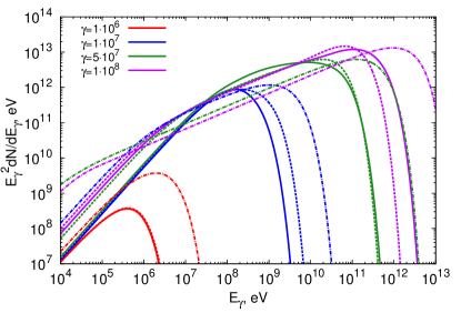
Figure 1.— The cumulative (integrated along trajectory) radiation spectra of electrons calculated for the outer gap model of the pulsar magnetosphere. The curves are obtained for different initial Lorenz factors of electrons $\gamma=10^{6},10^{7},5\times 10^{7},10^{8}$, and for different initial directions relative to the magnetic field lines: along the drift trajectory (solid lines), along the magnetic field line (dashed lines), and at pitch angle $\alpha=10\beta_{D}$ in the meridional plane opposite to the normal vector of magnetic field lines (dashed-dotted lines).

$\begin{array}[]{cc}\includegraphics[width=108.405pt]{ogq6t}&\includegraphics[width=108.405pt]{ogq7t}\\ \includegraphics[width=108.405pt]{ogq75t}&\includegraphics[width=108.405pt]{ogq8t}\end{array}$

Figure 2.— Time evolution of the $q$-parameter and the electron Lorenz factor in the outer gap model (complementary to Fig. 1). Four panels correspond to the initial Lorenz factor of electrons $\gamma=10^{6},10^{7},5\times 10^{7},10^{8}$ and their initial direction along the drift trajectory.

$\begin{array}[]{cc}\includegraphics[width=108.405pt]{ogq6a}&\includegraphics[width=108.405pt]{ogq7a}\\ \includegraphics[width=108.405pt]{ogq75a}&\includegraphics[width=108.405pt]{ogq8a}\end{array}$

Figure 3.— The same as in Fig.2, but for the initial direction of electrons along the magnetic field line.

$\begin{array}[]{cc}\includegraphics[width=108.405pt]{ogq6an}&\includegraphics[width=108.405pt]{ogq7an}\\ \includegraphics[width=108.405pt]{ogq75an}&\includegraphics[width=108.405pt]{ogq8an}\end{array}$

Figure 4.— The same as in Fig.2, but for the initial direction of electrons at an angle $10\beta_{D}$.

6.2. Polar Cap

In the polar cap model electrons radiate in the region located close to the surface of the neutron star where the magnetic field is much stronger than in the outer gap model, approaching to $B\approx 10^{12}$ G. This results in much faster damping of the perpendicular component of motion. The very small drift velocity $\beta_{D}$ implies that the drift trajectory and the magnetic field line almost coincide, thus even a small deflection from the magnetic field line produces radiation quite different from the curvature radiation. However, the transition to the curvature radiation regime occurs very fast. In the curvature regime, electrons radiate more energetic photons than in the outer gap model. But the curvature of the magnetic field lines in the polar cap model with $\theta_{0}\sim 1^{\circ}$ is only an order of magnitude larger than in the outer gap since the curvature of the dipole magnetic field scales as $\sim\sin\theta/r$. Correspondingly, the maximum energy of curvature radiation at the polar cap is only an order of magnitude higher than in the outer gap.

The energy spectra of radiation calculated for the polar cap model are shown in Fig. 5. The complementary plots for the evolution of the $q$-parameter and the electron Lorenz factor are presented in Figs. 6, 7, and 8. The initial position of the particle is $R_{0}=10^{6}$ cm, and $\theta_{0}=3^{\circ}$. The spectra indicated by solid lines correspond to the case when the initial direction of particle is along magnetic field line. In this case the radiation is in the curvature regime. But at the initial stage, the radiation proceeds in a very fast synchro-curvature regime, but abruptly turns to the regime with $q\approx 1$ and fast oscillations caused by fine gyrations.

The abrupt change of the regimes leads to an interesting feature in the cumulative spectra for the case of an initial pitch angle $\alpha_{0}=1/\gamma_{0}$ (dashed lines). Because of small changes in energy and fast change of the $q$-parameter, the energy spectra consist of two peaks. The peak at higher energies is produced by synchrotron radiation ($q\gg 1$, see Fig. 7), while the lower energy peak corresponds to curvature radiation regime. The double-peak structure disappears for large initial pitch angles. For example, for the pitch angle $100/\gamma_{0}$ the transition to the curvature regime is very fast, and the electron enters into this regime with dramatically reduced Lorentz factor. Thus the peak of the curvature radiation not only is shifted to smaller energies, but also is too weak to be seen in the cumulative spectrum.

In very strong magnetic fields, namely when the parameter $\chi=B\gamma\sin\alpha/B_{cr}\geq 1$, the radiation is produced in the quantum regime. Let’s assume that the initial pitch angle is inverse proportional to the initial Lorentz factor, $\alpha_{0}=a/\gamma_{0}$. This makes the condition of radiation in the quantum regime independent on $\gamma_{0}$:

$$\chi=\frac{B}{B_{cr}}\gamma\sin{\alpha_{0}}=\frac{1\cdot 10^{12}G}{2.94\cdot 10^{13}G}a\approx 3.4\cdot 10^{-2}a.$$ (31)

Thus, at the initial pitch angle with $a>30$, the electrons radiate in quantum regime. Dash-dotted lines in Fig. 5 present radiation spectra for the initial pitch-angles $\alpha_{0}=100/\gamma_{0}$. Note that in the quantum regime almost the entire energy of the parent electron is transferred to the radiated photon. Thus we should expect abrupt cutoff in the radiation spectra. This effect is clearly seen in Fig. 5 (dot-dashed curves corresponding to the initial pitch angle $\alpha_{0}=100/\gamma_{0}$). The gamma rays produced in the quantum regime are sufficiently energetic to be absorbed in the magnetic field through the $e^{+}e^{-}$ pair production. This will lead to the development of an electromagnetic cascade in the magnetic field. The spectrum of cascade gamma-rays that escape the pulsar magnetosphere will be quite different from the spectra shown in Fig. 5.

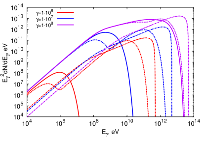
Figure 5.— The cumulative (integrated along trajectory) radiation spectra of electrons calculated for the outer gap model of the pulsar magnetosphere. The curves are obtained for different initial Lorenz factors of electrons $\gamma=10^{6},10^{7},10^{8}$, and for different initial directions relative to the magnetic field lines: along the magnetic field line (dashed lines), and for two pitch angles $1/\gamma_{0}$ (dashed lines) and $100/\gamma_{0}$ (dashed-dotted lines).

$\begin{array}[]{cc}\includegraphics[width=108.405pt]{pgq6al}&\includegraphics[width=108.405pt]{pgq7al}\end{array}$

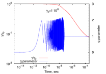
Figure 6.— Time evolution of the $q$-parameter and the electron Lorenz factor in the outer gap model (complementary to Fig. 5). Three panels correspond to the initial Lorenz factor of electrons $\gamma=10^{6},10^{7},10^{8}$ and their initial direction along the magnetic field line.

$\begin{array}[]{cc}\includegraphics[width=108.405pt]{pgq6an0}&\includegraphics[width=108.405pt]{pgq7an0}\end{array}$

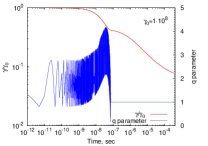
Figure 7.— The same as in Fig.6, but for the initial direction of electrons at pitch angle $1/\gamma_{0}$.

$\begin{array}[]{cc}\includegraphics[width=108.405pt]{pgq6an2}&\includegraphics[width=108.405pt]{pgq7an2}\end{array}$

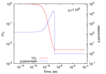
Figure 8.— The same as in Fig.6, but for the initial direction of electrons at pitch angle $100/\gamma_{0}$.

6.3. Protons in the Black Hole magnetosphere

The acceleration of the protons to ultrahigh energies in the potential gap of the spinning supermassive black hole should be accompanied by curvature radiation in the magnetic field which threads the black hole (Levinson (2000), Aharonian et al. (2002)). Here we briefly examine the radiation regimes and the gamma ray spectra of accelerated protons produced in this model. As before, we consider the radiation in the dipole magnetic field adopting the following (typical for a SMBH) parameters $B_{*}=10^{4}$ G and $R_{*}=10^{14}$ cm. The initial position of the particle is set at the polar angle $\theta_{0}=5^{\circ}$ relative to the magnetic dipole axis.

The larger (compared to electron) mass of proton leads to the larger drift velocity $\beta_{D}$. Therefore the spectra and the radiation regimes in the case of protons are less sensitive to the initial direction of motion. The radiation of protons deviates from the curvature radiation when the perpendicular component of proton’s Lorentz factor exceed

$$\gamma_{\perp}=\gamma\beta_{D}=\frac{m_{p}c^{2}\gamma^{2}}{eBr_{0}}=2.7\cdot 10^{7}\left(\frac{\gamma}{10^{10}}\right)^{2}\ .$$ (32)

This is larger by the factor of $m_{p}/m_{e}\approx 2\cdot 10^{3}$ compared to the same condition for electrons. It is interesting to note that for the same Lorenz factor, in the synchrotron regime protons radiates much weaker than electrons, whereas in the curvature regime they radiate equally.

The radiation spectra of protons with different initial pitch angles are presented in Fig. 9. The smallest angle $\alpha_{0}$ is close to $\beta_{D}$, and the proton radiates in the synchro-curvature regime (solid lines). Because of high energy the gyration period is large, and in the case of $\gamma_{0}=10^{10}$ the particle makes only several gyrations before escaping the region with high magnetic field (see Fig. 11). After that, the proton radiates with a very low rate, and the $q$-parameter approaches zero. In the case of $\gamma_{0}=10^{9}$, the proton gyrates more frequently (see Fig. 10) and there is seen more pronounced tendency of $q$ approaching to zero. The other curves correspond to the initial pitch angles $10\alpha_{0}$ and $100\alpha_{0}$. The spectra are shifted towards higher energies by the same factors of $q\approx 10$ and $q\approx 100$. Accordingly, for the Lorenz factor $\gamma_{0}=10^{11}$ which is not shown in figures, the proton will radiate predominantly in the curvature regime and the spectrum will be shifted by a factor of $(10^{11}/10^{10})^{3}=1000$ relative to the curvature spectrum of the proton with initial Lorenz factor $\gamma_{0}=10^{10}$. Despite the small energy losses relative to the initial energy, the amount of the radiated energy is quite large. As in the case of the pulsar polar cap model, for the chosen parameters the curvature radius of the magnetic field lines is larger by an order of magnitude compared to the gravitational radius of the black hole which usually is taken for evaluation of curvature radius. It yields smaller energy losses and increase the maximum Lorenz factor of acceleration compared to the case when the gravitational radius of the black hole is used as a curvature radius. To be more specific, the maximum Lorenz factor of a particle in radiative-loss limited regime scales with curvature radius $R_{c}$ as $\sqrt{R_{c}/R_{*}}$ (Aharonian et al. (2002), Levinson (2000)).

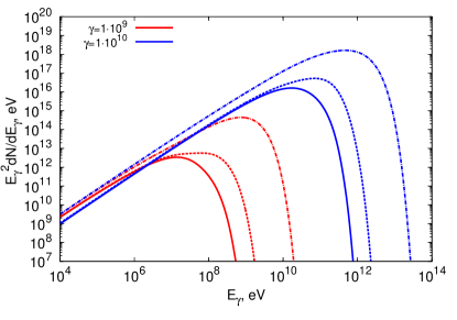
Figure 9.— The cumulative (integrated along trajectory) radiation spectra of protons in the magnetic field of rotating supermassive black hole. The chosen parameters are described in the text. The spectra correspond to two different Lorentz factors and three different initial pitch angles relative to the magnetic field lines: $10^{-4}$ (solid), $10^{-3}$ (dashed), $10^{-2}$ (dash-dotted) radian for $\gamma_{0}=10^{9}$ (red) and $10^{-3}$ (solid), $10^{-2}$ (dashed), $10^{-1}$ (dash-dotted) radian for $\gamma_{0}=10^{10}$ (blue).

$\begin{array}[]{cc}\includegraphics[width=108.405pt]{BHg9an1e5}&\includegraphics[width=108.405pt]{BHg9an1e6}\end{array}$

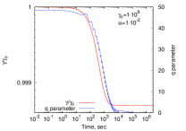
Figure 10.— Time-evolution of the Lorenz factor and the $q$-parameter in the magnetic field of a supermassive black hole with the initial Lorenz factor of protons $\gamma_{0}=10^{9}$ and their initial pitch angles $\alpha=10^{-4}$, $10^{-3}$, and $10^{-2}$.

$\begin{array}[]{cc}\includegraphics[width=108.405pt]{BHg10an1e7}&\includegraphics[width=108.405pt]{BHg10an1e8}\end{array}$

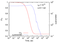
Figure 11.— Time-evolution of the Lorenz factor and the $q$-parameter in the magnetic field of a supermassive black hole with the initial Lorenz factor of protons $\gamma_{0}=10^{10}$ and their initial pitch angles $\alpha=10^{-3}$, $10^{-3}$, and $10^{-1}$.

7. Summary

The radiation of relativistic particles in a strong curved magnetic field is of a great astrophysical interest, in particular in the context of magnetospheric gamma-ray emission of rotation-powered pulsars. In these objects with very strong magnetic fields, the radiation proceeds in quite complex regimes, so it cannot be reduced merely to the consideration of the nominal synchrotron and curvature channels. For proper understanding of these radiation regimes and the transitions between them, the accurate treatment of the particle trajectory is a key issue. It can be done by solving the equations of motion taking into account energy losses of charged particles. In this work we followed this approach to explore the radiation features of ultrarelativistic particles in a dipole field which is a good approximation for the magnetic field structure in compact astrophysical objects. The accurate numerical solutions for the test particle trajectory allowed us to trace the radiation regimes and calculate self-consistently the radiation spectrum without any a priori assumption concerning the radiation regime.

In this paper we demonstrate that even small deflections of the initial particle motion from the magnetic field lines may result in a radiation spectrum quite different from the spectrum the curvature radiation. For any initial pitch angle, the particle tends, while losing its energy, to turn to the curvature radiation regime and to move strictly along drift trajectory (although never can achieve the latter). In principle, the fast increase of curvature of the magnetic field lines can turn the regimes in inverse order.

In different environments (or different positions relative to magnetic dipole) the transition to the curvature radiation regime proceeds with different rate. While in the polar cap model the transition occurs almost instantly, in the outer gap the transition could last so long that the particle would not turn to the curvature regime while passing the gap. The spectrum of the radiation becomes very different from the spectrum of the curvature radiation if the pitch angle of the particle is greater than drift speed $\beta_{D}=v_{D}/c$, and quite similar if it is smaller than $\beta_{D}$. For the typical parameters of the polar cap model, $\beta_{D}=2.2\cdot 10^{-9}(\gamma/10^{8})$. This implies that the even tiny deflection from the magnetic field line leads to the spectrum different from the curvature radiation spectrum.

Significant deviations of the radiation spectra from the nominal curvature radiation spectrum is expected also in the outer gap model. The particles do not move along magnetic field lines but gyrate around drift trajectory. This results in a different (more “energetic”) spectrum from the conventional curvature radiation spectrum. In the outer gap model, electrons with initial direction along magnetic field line start to radiate in the synchro-curvature regime, when the both the curvature of the magnetic field and its strength play equally important role. The effect is quite significant at large Lorentz factors of electrons, $\gamma\geq 10^{7}$.

Finally, we demonstrate the strong impact of the initial pitch angle on the radiation spectrum in the scenario of acceleration and motion of ultrahigh energy protons in the magnetosphere of a supermassive black hole.

Appendix A Energy losses in the quantum regime

In a very strong magnetic field, the ultrarelativistic electrons can radiate in the quantum regime, provided that

$$\chi=\frac{B}{B_{cr}}\gamma\sin\alpha\gtrsim 1,$$ (A1)

where $B_{cr}=\frac{2m^{2}c^{3}}{3e\hbar}\approx 2.94\cdot 10^{13}$ G. The energy lose rate can be written in the form (Bayer et al., 1973; Berestetskii et al., 1982)

$$\left|\frac{dE}{dt}\right|=\frac{e^{2}m^{2}c^{3}}{\sqrt{3}\pi\hbar^{2}}\overline{H}(\chi)\,,$$ (A2)

where

$$\overline{H}(\chi)=\int_{0}^{1}H(\tau,\chi)d\tau\ ,$$ (A3)

and

$$H(\tau,\chi)=\chi\left[(1-\tau)F(x)+x\tau^{2}K_{2/3}(x)\right],\quad x=\frac{\tau}{\chi(1-\tau)},$$ (A4)

where $K_{2/3}(x)$ is the modified Bessel function of the order $2/3$, $F(x)$ is the emissivity function of the synchrotron radiation (see Eq. 20), $\tau=\epsilon/E$, where $\epsilon$ is the energy of the radiated photon, $E$ is the energy of the radiating particle.

For calculations it is convenient to express $\overline{H}(\chi)$ in Eq.(A2) in a simple approximate analytical form. Using asymptotics of this function

$$\begin{aligned} &\overline{H}(\chi)\approx{\frac{8\pi\sqrt{3}}{27}}{\chi}^{2},\quad\chi\ll 1,\\ &\overline{H}(\chi)\approx{\frac{32\pi\sqrt{3}}{243}}{2}^{2/3}\Gamma\!\left(\frac{2}{3}\right)\chi^{2/3},\quad\chi\gg 1.\end{aligned}$$ (A5)

we have found the following approximation

$$\overline{H}(\chi)\approx\frac{8\pi\sqrt{3}}{27}\frac{\chi^{2}}{\left({\displaystyle 1+\frac{3}{4}\frac{(2\chi)^{2/3}}{\sqrt{\Gamma\!\left(\frac{2}{3}\right)}}}\right)^{2}}\times\left(1+\frac{0.52\sqrt{\chi}(1+3\sqrt{\chi}-3.2\chi)}{1+0.3\sqrt{\chi}+17\chi+11\chi^{2}}\right)$$ (A6)

The first two terms (before the sign $\times$) of Eq. (A6) give right asymptotics at $\chi\ll 1$ and $\chi\gg 1$ and provide an accuracy better than $10\%$ for other values of $\chi$, whereas the inclusion of the last term in the brackets makes the accuracy better than $0.1\%$ for any $\chi$.

The spectrum of the radiation in the quantum regime is expressed as

$$F_{q}(x,\tau) =(1-\tau)F(x)+\tau^{2}xK_{2/3}(x),\quad x =\frac{\tau}{1-\tau}\frac{E}{\epsilon_{c}},$$ (A7)

where $\epsilon_{c}=\frac{3e\hbar B\sin\alpha}{2mc}\gamma^{2}$ is the characteristic energy of the emitted photon. To use this function in Eq. (18), the $\epsilon_{c}$ should be changed to $\hbar\omega_{*}$. An analytical approximation of this function can be obtained using the approximation for emissivity function of the synchrotron radiation (Aharonian et al., 2010)

$$F(x)\approx 2.15x^{1/3}(1+3.06x)^{1/6}\frac{1+0.884x^{2/3}+0.471x^{4/3}}{1+1.64x^{2/3}+0.974x^{4/3}}e^{-x},$$ (A8)

and

$$xK_{2/3}(x)\approx 1.075x^{1/3}(1+3.72x)^{1/6}\frac{1+1.58x^{2/3}+3.97x^{4/3}}{1+1.53x^{2/3}+4.25x^{4/3}}e^{-x}.$$ (A9)

Both approximations provide an accuracy better than $0.2\%$ for any value of the argument $x$.

References

- Kelner and Aharonian (2012) S. Kelner and F. Aharonian, ArXiv e-prints (2012), arXiv:1207.6903 [astro-ph.HE] .
- Alfven and Falthammar (1963) H. Alfven and C. G. Falthammar, Cosmical Electrodynamics (Oxford University Press, 1963).
- Landau and Lifshitz (1975) L. D. Landau and E. M. Lifshitz, The Classical Theory of Fields (Butterworth-Heinemann, Oxford, 1975).
- Cheng et al. (1986) K. S. Cheng, C. Ho, and M. Ruderman, ApJ 300, 500 (1986).
- Trubnikov (2000) B. A. Trubnikov, Soviet Journal of Experimental and Theoretical Physics 91, 479 (2000).
- Schwinger (1949) J. Schwinger, Phys. Rev. 75, 1912 (1949).
- Berestetskii et al. (1982) V. B. Berestetskii, E. M. Lifshitz, and L. P. Pitaevskii, Quantum Electrodynamics (Butterworth-Heinemann, Oxford, 1982).
- Takata et al. (2004) J. Takata, S. Shibata, and K. Hirotani, MNRAS 354, 1120 (2004), arXiv:astro-ph/0408044 .
- Hirotani (2008) K. Hirotani, ApJ 688, L25 (2008), arXiv:0810.0865 .
- Levinson (2000) A. Levinson, Physical Review Letters 85, 912 (2000).
- Levinson and Rieger (2011) A. Levinson and F. Rieger, ApJ 730, 123 (2011), arXiv:1011.5319 [astro-ph.HE] .
- Aharonian et al. (2002) F. A. Aharonian, A. A. Belyanin, E. V. Derishev, V. V. Kocharovsky, and V. V. Kocharovsky, Phys. Rev. D 66, 023005 (2002), arXiv:astro-ph/0202229 .
- Bayer et al. (1973) V. N. Bayer, V. M. Katkov, and V. S. Fadin, Radiation of Relativistic Electrons (Atomizdat, Moscow, 1973).
- Aharonian et al. (2010) F. A. Aharonian, S. R. Kelner, and A. Y. Prosekin, Phys. Rev. D 82, 043002 (2010), arXiv:1006.1045 [astro-ph.HE] .