Intrinsic plasmons in 2D Dirac materials

Abstract

We consider theoretically, using the random phase approximation (RPA), low-energy intrinsic plasmons for two-dimensional (2D) systems obeying Dirac-like linear chiral dispersion with the chemical potential set precisely at the charge neutral Dirac point. The “intrinsic Dirac plasmon” energy has the characteristic $\sqrt{q}$ dispersion in the 2D wave-vector $q$, but vanishes as $\sqrt{T}$ in temperature for both monolayer and bilayer graphene. The intrinsic plasmon becomes overdamped for a fixed $q$ as $T\rightarrow 0$ since the level broadening (i.e. the decay of the plasmon into electron-hole pairs due to Landau damping) increases as $1/\sqrt{T}$ as temperature decreases, however, the plasmon mode remains well-defined at any fixed $T$ (no matter how small) as $q\rightarrow 0$. We find the intrinsic plasmon to be well-defined as long as $q<\frac{k_{B}T}{e^{2}}$. We give analytical results for low and high temperatures, and numerical RPA results for arbitrary temperatures, and consider both single-layer and double-layer intrinsic Dirac plasmons. We provide extensive comparison and contrast between intrinsic and extrinsic graphene plasmons, and critically discuss the prospects for experimentally observing intrinsic Dirac point graphene plasmons.

I Introduction

Collective plasma oscillations of free carriers in doped or gated grapheneHwang and Das Sarma (2007) (we would refer to this situation as “extrinsic” graphene where the chemical potential or the Fermi level is doped away from the Dirac point) have attracted considerable interest both from fundamental and technological perspectivesVafek (2006); Ryzhii et al. (2007); Gangadharaiah et al. (2008); Polini et al. (2008); Liu et al. (2008); Kramberger et al. (2008); Lu et al. (2009); Jablan et al. (2009); Das Sarma and Hwang (2009); Stauber et al. (2010); Langer et al. (2010); Liu and Willis (2010); Tudorovskiy and Mikhailov (2010); Hwang et al. (2010); Mishchenko et al. (2010); Muniz et al. (2010); Koch et al. (2010); Schütt et al. (2011); Politano et al. (2011); Villegas and Tavares (2011); Abedinpour et al. (2011); Walter et al. (2011); Tegenkamp et al. (2011); Gan et al. (2012); Gómez-Santos and Stauber (2012); Dong et al. (2012); Krstajić and Peeters (2012a, b); Langer et al. (2012); Politano et al. (2012); Gorbach (2013); Zhu et al. (2013). The fundamental interest arises from the fact that graphene plasmons are apriori quantum-mechanical entities with no classical analogs whatsoeverDas Sarma and Hwang (2009) (since in classical physics energy is always proportional to the square of the momentum and never has a linear dispersion as in graphene). This is manifested in the fact that the long wave-length plasma dispersion relation in extrinsic graphene goes as $\omega_{p}=\sqrt{2r_{s}\hbar v_{F}qE_{F}}$, where $E_{F}=\hbar v_{F}k_{F}=\hbar v_{F}\sqrt{\pi n}$ is the Fermi energy (i.e. the chemical potential at $T=0$) associated with a doping carrier density of $n$ and $v_{F}$ is the (constant) graphene velocity defining the linear energy dispersion, and $r_{s}=e^{2}/(\kappa\hbar v_{F})$ is the so-called graphene fine-structure constant (defining the dimensionless strength of Coulomb interaction with $\kappa$ being the background lattice dielectric constant), with an “$\hbar$” appearing explicitly in the definition of the plasma frequency ($\omega_{p}=\sqrt{2e^{2}qv_{F}\hbar\sqrt{\pi n}/\kappa}$ in terms of the experimentally controlled variables $q$, $n$, and $\kappa$). This is in sharp contrast to the corresponding parabolic dispersion systemsDas Sarma and Hwang (1998); Hwang and Das Sarma (2001) with an effective mass $m$ where $\omega_{p}$ ($\propto\sqrt{\dfrac{ne^{2}}{\kappa m}}$) is the same classically or quantum-mechanically in the long wavelength ($q\rightarrow 0$) limit in any dimensionality. The technological interest arises from the considerable recent progress in graphene nanoplasmonicsKoppens et al. (2011); Nikitin et al. (2011); Ju et al. (2011); Echtermeyer et al. (2011); Fei et al. (2011); Yan et al. (2012); Grigorenko et al. (2012); Fei et al. (2012); Chen et al. (2012); Thongrattanasiri et al. (2012); Davoyan et al. (2012); Zhan et al. (2012); Carbotte et al. (2012); Ilic et al. (2012); Rast et al. (2013) for prospective optoelectronic applicationsXia et al. (2009); Xu et al. (2010); Mueller et al. (2010); Rana (2011); Rana et al. (2011); Liu et al. (2011); Sun et al. (2010); Bonaccorso et al. (2010); Vakil and Engheta (2011); Bao and Loh (2012).

In contrast to the extensively studied extrinsic graphene plasmons, there has been little interest in the collective modes of intrinsic or undoped graphene, where the chemical potential sits right at the Dirac point with a completely filled valence band a completely empty conduction band at $T=0$. (Our interest here is in low-energy $\sim$ meV two-dimensional collective modes and not very high-energy $\sim 10$ eV band- or so-called $\pi$- plasmons where the whole valence band charge response is involvedEberlein et al. (2008); Yuan et al. (2011); Shin et al. (2011); Yan et al. (2011); Kinyanjui et al. (2012); Despoja et al. (2013).) By definition, the doping carrier density vanishes at the Dirac point with $n=0$ ($\propto k_{F}\propto E_{F}$), and the extrinsic graphene dispersion relation, $\omega_{p}\propto n^{1/4}$, implies that no intrinsic graphene plasmons (or more generally, Dirac plasmons) are possible.

The above is certainly true strictly at $T=0$ where there can be no free carriers for $E_{F}=0$. But, for non-zero temperatures, $T\neq 0$, the gapless nature of graphene leads to a thermal population of electrons (in the conduction band) and holes (in the valence band) with equal density ($n_{e}=n_{h}=n$). This thermal electron-hole excitation process is known to be a power law (in fact $n\propto T^{2}$) due to the gaplessness of grapheneHwang and Das Sarma (2009). Putting $n\propto T^{2}$ in the formula for the graphene extrinsic plasma frequency, we conclude that there should be a finite-temperature intrinsic graphene plasmon with a long-wavelength plasma frequency going as $\omega_{p}\sim\sqrt{qT}$. But, finite temperature implies that the collective mode will decay into electron-hole pairs even at long wavelength, and therefore, such an intrinsic Dirac plasmon may be ill-defined even for $q\rightarrow 0$ since its decay (i.e. damping) rate (or level broadening) $\gamma$ could exceed the mode frequency $\omega_{p}$ making the mode an overdamped excitation of little interest.

In the current work, we theoretically study intrinsic Dirac plasmons for both monolayer and bilayer graphene and for single- and double-layer systems. We obtain both asymptotic theoretical analytical results at long wavelengths and low/high temperatures, and quantitative numerical results for arbitrary wavevectors and temperatures. We use the RPA approach which should be well-valid for graphene plasmons at arbitrary wavevectors by virtue of its relatively small value of $r_{s}$ ($\lesssim 1$ typically). We compare and contrast the temperature dependence of intrinsic and extrinsic graphene plasmon frequency (and their Landau damping) in order to comment on the feasibility of the experimental observation of our theoretical predictions. The possible existence of high-temperature intrinsic graphene plasmons (with $E_{F}=0$) is a qualitative difference between graphene and gapped 2D semiconductor-based electron/hole systems.

II Theory and results

Within the RPA, the collective plasmon modes of an electron system are given by the zeros of the complex dielectric function $\varepsilon(q,\omega)$:

$$\varepsilon(q,\omega)=1-V(q)\Pi(q,\omega)=0$$ (1)

where $V(q)$ is the relevant bare electron-electron (i.e. Coulomb) interaction and $\Pi(q,\omega)$ is the noninteracting polarizability of the system. (As an aside we note that $\varepsilon(q,\omega)=1-V(q)\Pi(q,\omega)$) is the exact expression for the microscopic dielectric function if $\Pi(q,\omega)$ is the exact interacting irreducible polarizability function which, of course, is unknown — RPA consists of replacing the exact $\Pi(q,\omega)$ by the corresponding non-interacting or bare polarizability function.) Equation (1), as it stands, applies for a single-component (i.e. single-layer in our case) system — for the double-layer case $\varepsilon(q,\omega)$ should be interpreted as a matrix in the layer index with Eq. (1) being interpreted as a determinantal equation $|1-V\Pi|=0$.

In general, Eq. (1) will have complex solutions in frequency, $\omega=\omega_{p}(q)+i\gamma(q)$, with $\omega_{p}$ and $\gamma$ being respectively the collective mode (i.e. plasma) frequency (which we will often refer to as the plasmon) and its damping. If $\omega_{p}\gg\gamma$, the plasmon collective mode is well-defined, and by contrast for $\gamma\gtrsim\omega_{p}$, the plasmon is heavily damped (or even overdamped) and is not particularly relevant experimentally as a self-sustaining normal mode of the system.

Before proceeding with the theoretical details for intrinsic graphene collective modes, we write down the full formal expression for the graphene non-interacting polarizabilityHwang and Das Sarma (2007); Wunsch et al. (2006) to be used in Eq. (1):

$$\Pi(q,\omega)=-\frac{4}{A}\underset{\mathbf{k},s,s^{\prime}}{\sum}\frac{f_{s,\mathbf{k}}-f_{s^{\prime},\mathbf{k^{\prime}}}}{\omega+\epsilon_{s,\mathbf{k}}-\epsilon_{s^{\prime},\mathbf{k^{\prime}}}+i\eta}F_{s,s^{\prime}}(\mathbf{k},\mathbf{k^{\prime}})$$ (2)

where $A$ is the area of the 2D layers and the factor of $4$ arises from the valley/spin degeneracy (two each) of graphene. In Eq. (2), $\mathbf{k^{\prime}\equiv k+q}$ and $s,s^{\prime}=\pm 1$ with $F_{s,s^{\prime}}(\mathbf{k,k^{\prime}})=(1+\cos\theta)/2$ arising from the matrix element effect associated with the chiral nature of Dirac fermions. The functions $\epsilon_{s,\mathbf{k}}$, $\epsilon_{s^{\prime},\mathbf{k^{\prime}}}$ are single-particle energies for wavevector $\mathbf{k}$, $\mathbf{k^{\prime}}$ respectively, and $f_{s,\mathbf{k}}$, $f_{s^{\prime},\mathbf{k^{\prime}}}$ are the corresponding non-interacting Fermi distribution functions. We mention that explicit forms for the polarizability function in monolayer and bilayer graphene were derived in Refs. [Hwang and Das Sarma, 2007] and [Sensarma et al., 2010] respectively at the zero temperature. The finite-temperature polarizability, which cannot be obtained in a closed analytic form for arbitrary $T$, can be directly obtained from Eq. (2) using finite-temperature Fermi distribution functions or (numerically more conveniently) by using the following integral identity to obtain the finite-$T$ polarizability from its known analytic formHwang and Das Sarma (2007) at $T=0$

$$\Pi(q,\omega,\mu;T)=\int_{0}^{\infty}d\mu^{\prime}\dfrac{\Pi(q,\omega,\mu^{\prime};T=0)}{4k_{B}T\text{cosh}^{2}[(\mu-\mu^{\prime})/2k_{B}T]}$$ (3)

We also note that the 2D Coulomb interaction is given by:

$$V(q)=\dfrac{2\pi e^{2}}{\kappa q}e^{-q|z|}$$ (4)

where $z=0$ for single-layer systems and $|z|=d$, where $d$ is the interlayer separation for double layer systems.

II.1 Monolayer graphene

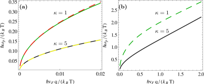
Figure 1: (Color online). Plasmon dispersion of intrinsic MLG. (a) presents the plasmon dispersion in the high temperature regime ($k_{B}T\gg\hbar v_{F}q$). The dashed and solid lines correspond to the analytical results (given in Eq. (7)) and the numerical results, respectively. (b) Numerical results for the plasmon dispersion as a function of $\hbar v_{F}q/(k_{B}T)$. The dashed and solid lines correspond to $\kappa=1$ and $\kappa=5$, respectively.

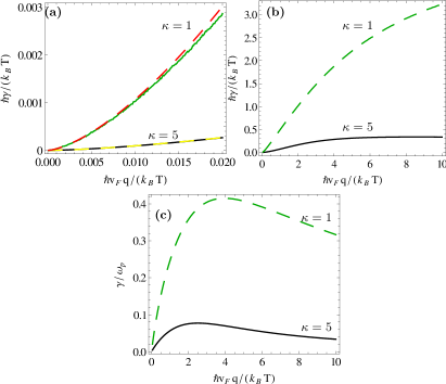
Figure 2: (Color online). Plasmon damping rate of intrinsic MLG. (a) presents the plasmon damping rate in the high temperature regime ($k_{B}T\gg\hbar v_{F}q$). The dashed and solid lines correspond to the analytical results (given in Eq. (8)) and the numerical results, respectively. (b) Numerical results for $\hbar\gamma/(k_{B}T)$ as a function of $\hbar v_{F}q/(k_{B}T)$. (c) $\gamma_{p}/\omega$ as a function of $\hbar v_{F}q/(k_{B}T)$. The dashed and solid lines correspond to $\kappa=1$ and $\kappa=5$, respectively.

We first consider the intrinsic plasmon modes in monolayer graphene (MLG). We use units such that $\hbar=1$ throughout so that frequency/energy and wavevector/momentum have the same units in our notations.

For intrinsic graphene, there are no free carriers at zero temperature and the chemical potential $\mu$ is precisely at the Dirac point: $\mu=0$. We note that this is true even for $T\neq 0$, i.e. $\mu(T)=\mu(0)=E_{F}=0$ for intrinsic graphene, by definition. The zero-temperature polarizability $\Pi(q,\omega)$ for intrinsic graphene is $-\frac{q^{2}}{4\sqrt{v_{F}^{2}q^{2}-(\omega+i0)^{2}}}$ as given in Ref. [Hwang and Das Sarma, 2007]. Since the real part of $V(q)\Pi(q,\omega)$ is pure negative, there can be no 2D plasmon modes in intrinsic graphene within RPA at $T=0$ according to Eq. (1). Thus our work on intrinsic Dirac plasmons, using RPA, focuses entirely on finite temperature collective modes in undoped intrinsic graphene.

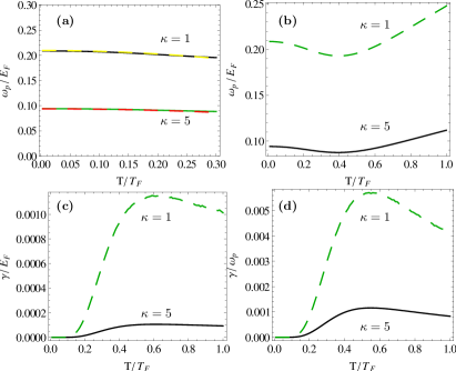
Figure 3: (Color online). Results for extrinsic MLG with $q/k_{F}=0.01$. (a) presents the plasmon dispersion in the low temperature regime. The dashed and solid lines correspond to the analytical results (given in Eq. (11)) and the numerical results, respectively. (b) Numerical results for $\omega_{p}/E_{F}$ as a function of $T/T_{F}$. (c) Numerical results for $\gamma/E_{F}$ as a function of $T/T_{F}$. (d) Numerical results for $\gamma/\omega_{p}$ as a function of $T/T_{F}$. The dashed and solid lines correspond to $\kappa=1$ and $\kappa=5$, respectively.

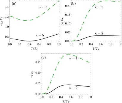
Figure 4: (Color online). Results for extrinsic MLG with $q/k_{F}=0.5$. (a) Numerical results for $\omega_{p}/E_{F}$ as a function of $T/T_{F}$. (b) Numerical results for $\gamma/E_{F}$ as a function of $T/T_{F}$. (c) Numerical results for $\gamma/\omega_{p}$ as a function of $T/T_{F}$. The dashed and solid lines correspond to $\kappa=1$ and $\kappa=5$, respectively.

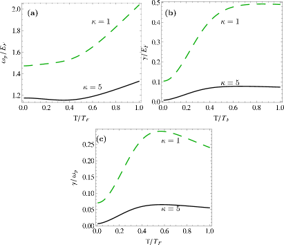
Figure 5: (Color online). Results for extrinsic MLG with $q/k_{F}=1.0$. (a) Numerical results for $\omega_{p}/E_{F}$ as a function of $T/T_{F}$. (b) Numerical results for $\gamma/E_{F}$ as a function of $T/T_{F}$. (c) Numerical results for $\gamma/\omega_{p}$ as a function of $T/T_{F}$. The dashed and solid lines correspond to $\kappa=1$ and $\kappa=5$, respectively.

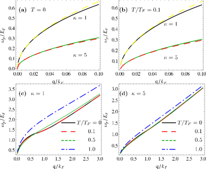
Figure 6: (Color online). Plasmon dispersion as a function of $q/k_{F}$ for extrinsic MLG. (a) and (b) present $\omega_{p}/E_{F}$ in the long wavelength limit. The dashed and solid lines correspond to the analytical results (given in Eq. (12)) and the numerical results, respectively. (a) is for $T=0$ and (b) is for $T/T_{F}=0.1$. (c) and (d) present $\omega_{p}/E_{F}$ for different temperatures. (c) is for $\kappa=1$ and (d) is for $\kappa=5$.

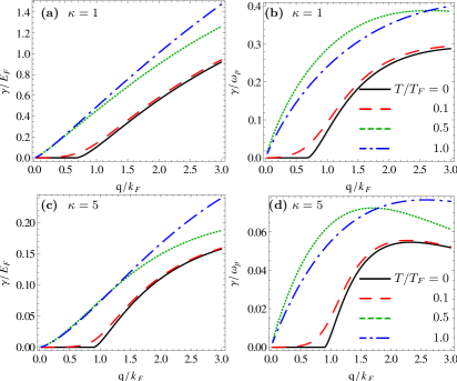
Figure 7: (Color online). Plasmon damping rate as a function of $q/k_{F}$ for extrinsic MLG. (a) and (c) $\gamma/E_{F}$ as a function of $q/k_{F}$ for different temperatures. (b) and (d) present $\gamma/\omega_{p}$ as a function of $q/k_{F}$. (a) and (b) are for $\kappa=1$; (c) and (d) are for $\kappa=5$. Note that the legend applies to all sub-figures.

Putting $\mu=0$ and taking the long-wavelength limit $v_{F}q/k_{B}T\rightarrow 0$, we get from Eqs. (1) and (2) the following expression for the finite-temperature ($k_{B}T/v_{F}q\gg 1$) intrinsic graphene polarizability function (We mention that the complete analytical $\Pi(q,\omega)$ at $T=0$ for both intrinsic and extrinsic case, i.e. intraband and interband, can be found in Ref. [Hwang and Das Sarma, 2007]):

$$\Pi(q,\omega)\approx\frac{2\ln 2}{\pi}\frac{q^{2}}{\omega^{2}}k_{B}T+\frac{i}{16}\frac{q^{2}}{\sqrt{\omega^{2}-q^{2}v_{F}^{2}}}\frac{\omega}{k_{B}T}$$ (5)

which reduces to (in the limit $\omega\gg qv_{F}$ as $q\rightarrow 0$):

$$\Pi(q,\omega)\approx\frac{2\ln 2}{\pi}\frac{q^{2}}{\omega^{2}}k_{B}T+\frac{i}{16}\frac{q^{2}}{k_{B}T}$$ (6)

Putting Eq. (6) in Eq. (1), and solving for the complex frequency defining the intrinsic plasmon, we get:

$$\omega_{p} = \sqrt{(4\ln 2)r_{s}\hbar v_{F}qk_{B}T}$$ (7)

$$\gamma = \frac{\pi\hbar v_{F}qr_{s}}{8\sqrt{k_{B}T}}\sqrt{(\ln 2)r_{s}\hbar v_{F}q}$$ (8)

We have restored $\hbar$ in Eqs. (7) and (8) for the sake of clarity and usefulness (and $r_{s}=e^{2}/\kappa\hbar v_{F}$ is the graphene fine-structure constant).

Equations (7) and (8) define the long-wavelength (and necessarily finite temperature) intrinsic MLG plasmon, which is determined by the variables temperature and wavevector (and not by any carrier density $n$ as in all ordinary plasmon modes). We note that $\omega_{p},\gamma\rightarrow 0$ as $q\rightarrow 0$, but obeying different power laws: $\omega_{p}\sim\sqrt{q}$ consistent with the 2D plasmon behavior and $\gamma\sim q^{3/2}$. We also note that $\omega_{p}\sim\sqrt{T}$ and $\gamma\sim 1/\sqrt{T}$ whereas $\omega_{p}\sim\sqrt{r_{s}}$ and $\gamma\sim r_{s}^{3/2}$ with $r_{s}\sim\kappa^{-1}$ giving the dependence on the background dielectric constant.

We note that $\omega_{p}/\gamma=16\kappa k_{B}T/(\pi e^{2}q)$ from Eqs. (7) and (8), and therefore the long-wavelength intrinsic plasmon is well-defined as long as

$$q<\frac{16\kappa k_{B}T}{\pi e^{2}}$$ (9)

which defines the condition for the existence of a well-defined long-wavelength intrinsic MLG plasmon. Thus, the intrinsic plasmon remains well-defined at long-wavelength for arbitrarily low temperature as long as one is probing wavevectors shorter than the critical wavevector $q_{c}$ defined by

$$q_{c}=\frac{16\kappa k_{B}T}{\pi e^{2}}$$ (10)

For $q<q_{c}$, the MLG intrinsic plasmon exists as a well-defined long wavelength collective mode, and for $q>q_{c}$, it is overdamped (i.e. $\gamma>\omega_{p}$).

Before providing our full numerical results for the MLG intrinsic plasmon for arbitrary $q$ and $T$, we briefly compare the analytical results for intrinsic and extrinsic MLG plasmons, which were earlier considered in Refs. [Hwang and Das Sarma, 2007] and [Das Sarma and Hwang, 2009]. The $T=0$ plasmon dispersion for extrinsic (i.e. doped) graphene is given in the long wavelength limit by:

$$\omega_{p}=\left(2r_{s}\hbar v_{F}qE_{F}\right)^{1/2}=\left(\frac{2e^{2}\hbar v_{F}q}{\kappa}\sqrt{\pi n}\right)^{1/2}$$ (11)

where $n$ is the carrier density (with a Fermi level $E_{F}=\hbar v_{F}\sqrt{\pi n}\neq 0$). It is easy to obtain the low-temperature analytical result for the MLG plasmon dispersion by using the finite-temperature expansion for the chemical potential: $\mu(T)\approx E_{F}\left[1-\frac{\pi^{2}}{6}\left(\frac{T}{T_{F}}\right)^{2}\right]$ for $T\ll T_{F}=E_{F}/k_{B}$. We get for $T\ll T_{F}$:

$$\omega_{p}=\left(2r_{s}\hbar v_{F}qE_{F}\left[1-\frac{\pi^{2}}{6}\left(\frac{T}{T_{F}}^{2}\right)\right]\right)^{1/2}$$ (12)

Thus, $\omega_{p}(T)=\omega_{p}(T=0)\left[1-\frac{\pi^{2}}{12}\left(\dfrac{T}{T_{F}}\right)^{2}\right]$, which is a small correction to the $T=0$ result. We note that the Landau damping for extrinsic plasmons at long wavelengths and low temperatures is exponentially suppressed, going as $e^{-T/T_{F}}$. We remark here that the reason that the finite-$T$ extrinsic plasmon is exponentially weak by Landau damped (as $T\rightarrow 0$) whereas the corresponding intrinsic plasmon has power law ($\gamma\sim 1/\sqrt{T}$) divergent Landau damping as $T\rightarrow 0$ is that, by definition, the intrinsic plasmon is always in the high-temperature regime for any temperatures since $E_{F}=k_{B}T_{F}=0$ for intrinsic plasmons. (Below we will discuss the high-temperature limit for the extrinsic plasmon.)

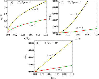
Figure 8: (Color online). Results for extrinsic MLG with $T/T_{F}=10.0$. (a) presents plasmon dispersion in the long wavelength limit. The dashed and solid lines correspond to the analytical results (given in Eq. (17)) and the numerical results, respectively. (b) Plasmon damping rate versus $q/k_{F}$. The dashed and solid lines correspond to the analytical results (given in Eq. (18)) and the numerical results, respectively. (c) $\gamma/\omega_{p}$ versus $q/k_{F}$. The dashed and solid lines correspond to the analytical results (given in Eq. (17)) and the numerical results, respectively.

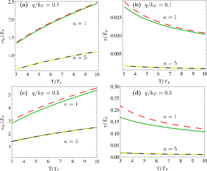
Figure 9: (Color online). Results for extrinsic MLG. (a) and (c) present plasmon dispersion versus $T/T_{F}$. The dashed and solid lines correspond to the analytical results (given in Eq. (17)) and the numerical results, respectively. (b) and (d) present plasmon damping rate versus $T/T_{F}$. (a) and (b) are for $q/k_{F}=0.1$. (c) and (d) are for $q/k_{F}=0.5$. The dashed and solid lines correspond to the analytical results (given in Eq. (18)) and the numerical results, respectively.

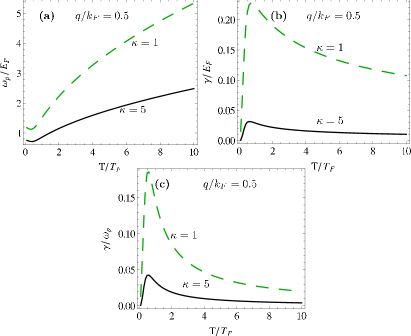
Figure 10: (Color online). Results for extrinsic MLG with $q/k_{F}=0.5$ over a wide $T/T_{F}=0-10$ range. (a) Numerical results for $\omega_{p}/E_{F}$ as a function of $T/T_{F}$. (b) Numerical results for $\gamma/E_{F}$ as a function of $T/T_{F}$. (c) Numerical results for $\gamma/\omega_{p}$ as a function of $T/T_{F}$. The dashed and solid lines correspond to $\kappa=1$ and $\kappa=5$, respectively.

An interesting exercise (alluded to in the Introduction of this paper) is to ask whether the long-wavelength intrinsic plasmon dispersion (i.e. Eq. (7)) can be obtained from the corresponding extrinsic plasmon dispersion (i.e. Eq. (11)) by reinterpreting the doping carrier density $n$ in Eq. (11) as the thermally excited carrier density $n(T)$ for the intrinsic case. The thermally excited carrier density $n(T)$ for intrinsic graphene with the Fermi level at the Dirac point ($E_{F}=0$) is easily calculated to be:

$$n(T)=\int D(E)f(E)dE$$ (13)

where $D(E)=4E/(2\pi v_{F}^{2})$ is the graphene density of states. Integrating over the Fermi distribution function $f(E)$ at temperature $T$ with $\mu=0$ we get:

$$n(T)=\frac{\pi}{6}\frac{(k_{B}T)^{2}}{\hbar^{2}v_{F}^{2}}$$ (14)

Inserting Eq. (13) for $n$ in Eq. (11) we get:

$$\omega_{p}=\left[\left(2\sqrt{\dfrac{\pi^{2}}{6}}\right)r_{s}(\hbar v_{F}q)(k_{B}T)\right]^{1/2}$$ (15)

Eq. (15) has the same parameter dependence $\sqrt{r_{s}\hbar v_{F}qk_{B}T}$ as in the correct intrinsic plasmon dispersion given by Eq. (7) with the only difference is that the prefactor in Eq. (15) is $2\sqrt{\pi^{2}/6}\approx 2.6$ versus the prefactor in Eq. (7) is $4\ln 2\approx 2.8$. Thus, the plasma frequency is given by $1.67\sqrt{r_{s}\hbar v_{F}q(k_{B}T)^{1/2}}$ and by $1.60\sqrt{r_{s}\hbar v_{F}q(k_{B}T)^{1/2}}$ in Eq. (15).

We now consider the high-temperature limit of the extrinsic plasmon dispersion for gated or doped graphene taking $T\gg T_{F}(=E_{F}/k_{B})$. The asymptotic high-temperature expression for $\Pi(q,\omega)$ in doped graphene is given by (again for $qv_{F}\ll\omega$):

$$\Pi(q,\omega)\approx\frac{2\ln 2}{\pi}\frac{q^{2}}{\omega^{2}}k_{B}T\left(1+\frac{{T_{F}}^{4}}{128(\ln 2)^{3}T^{4}}\right)$$

$$+\frac{i}{16}\frac{q^{2}}{\sqrt{\omega^{2}-q^{2}}}\frac{\omega}{k_{B}T}\left(1-\frac{\omega^{2}}{48k_{B}^{2}T^{2}}\right)$$ (16)

We emphasize that Eq. (16) is valid for extrinsic graphene in the limit of $T\gg T_{F}$ and $qv_{F}\ll\omega$. Using Eq. (16) to solve for the plasmon modes in Eq. (1), we get:

$$\omega_{p} = \sqrt{4\ln 2\ r_{s}\hbar v_{F}qk_{B}T\left(1+\frac{{T_{F}}^{4}}{128(\ln 2)^{3}T^{4}}\right)}$$ (17)

$$\gamma = \frac{\pi\hbar v_{F}qr_{s}}{8\sqrt{k_{B}T}}\sqrt{\ln 2\ r_{s}\hbar v_{F}q}\left(1-\frac{\hbar v_{F}qr_{s}\ln 2}{12k_{B}T}\right)$$ (18)

A direct comparison between Eqs. (17), (18) and Eqs. (7), (8) show that the $T/T_{F}\rightarrow\infty$ limit of the extrinsic plasmon dispersion and broadening indeed agree with the corresponding intrinsic plasmon results in the leading order, as indeed it must. We mention, however, that this agreement is only in the $T/T_{F}\rightarrow\infty$ limit (i.e. the $T_{F}=0$ limit of the extrinsic situation). Thus, there is a correction to the leading-order extrinsic plasmon dispersion in Eq. (17) going as $O(T_{F}^{4}/T^{4})$ which, by definition, cannot exist in the intrinsic plasmon dispersion where the leading-order dispersion comes entirely as $\sqrt{qT}$ with no correction term in temperature. All higher-order temperature corrections to the intrinsic plasmon dispersion occur in higher-order terms in the wavevector $q$.

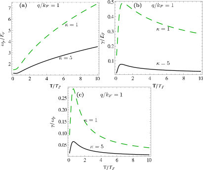
Figure 11: (Color online). Results for extrinsic MLG with $q/k_{F}=1.0$ over a wide $T/T_{F}=0-10$ range. (a) Numerical results for $\omega_{p}/E_{F}$ as a function of $T/T_{F}$. (b) Numerical results for $\gamma/E_{F}$ as a function of $T/T_{F}$. (c) Numerical results for $\gamma/\omega_{p}$ as a function of $T/T_{F}$. The dashed and solid lines correspond to $\kappa=1$ and $\kappa=5$, respectively.

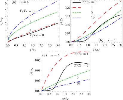
Figure 12: (Color online). Results for extrinsic MLG with $\kappa=5$. (a) Numerical results for $\omega_{p}/E_{F}$ as a function of $q/k_{F}$. (b) Numerical results for $\gamma/E_{F}$ as a function of $q/k_{F}$. (c) Numerical results for $\gamma/\omega_{p}$ as a function of $q/k_{F}$. The solid, dashed, dotted and dot-dashed lines correspond to $T/T_{F}=0,\ 1,\ 5$, and $10$, respectively.

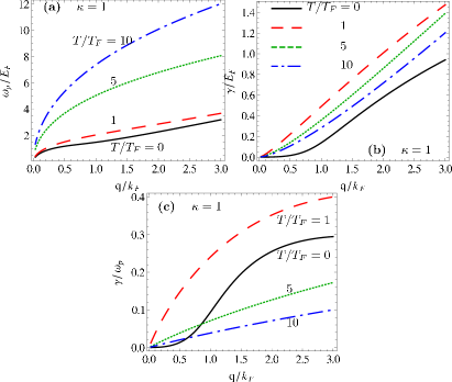
Figure 13: (Color online). Results for extrinsic MLG with $\kappa=1$. (a) Numerical results for $\omega_{p}/E_{F}$ as a function of $q/k_{F}$. (b) Numerical results for $\gamma/E_{F}$ as a function of $q/k_{F}$. (c) Numerical results for $\gamma/\omega_{p}$ as a function of $q/k_{F}$. The solid, dashed, dotted and dot-dashed lines correspond to $T/T_{F}=0,\ 1,\ 5$, and $10$, respectively.

We now present in Figs. 1 and 2 our calculated numerical results for the intrinsic graphene energy dispersion and level broadening for arbitrary values of wavevector $q$ and temperature $T$. (Our analytical results presented above in Eqs. (7) and (8) are necessarily restricted to the $\hbar v_{F}q\ll k_{B}T$ regime.) In presenting our results, we find that there are only two dimensionless (independent) variables that completely characterize the intrinsic graphene plasmon properties: $\kappa$, and $\hbar v_{F}q/k_{B}T$. In Figs. 1 and 2, we use two values of $\kappa=1$ (suspended graphene) and $5$ (graphene on boron nitride (BN) substrate) as representative examples of strongly ($\kappa=1$, i.e. $r_{s}\approx 2.2$) and weakly ($\kappa=5$, i.e. $r_{s}\approx 0.4$) interacting systems to show our numerical results for the numerically calculated plasmon energy $\hbar\omega_{p}$ and level broadening $\hbar\gamma$ in units of $k_{B}T$ as functions of the dimensionless 2D wavevector $\hbar v_{F}q/(k_{B}T)$. Our numerical results solve Eq. (1) to obtain the complex solution with the real part being the plasma frequency and the imaginary part the broadening. We obtain $\Pi(q,\omega)$ at arbitrary temperatures numerically in order to solve for the plasmon modes at arbitrary temperatures and wavevectors. In Fig. 1, the plasma frequency is shown as a function of wavevector, both for the small-$q$ regime and over a large range of $q$. The small-$q$ results serve to verify the accuracy of our asymptotic analytic result given in Eq. (7). In Fig. 2 we depict our calculated plasmon broadening as a function of wavevector again for small-$q$ (Fig. 2(a)) and extended-$q$ (Fig. 2(b)) regions whereas in Fig. 2(c) we depict the dimensionless ratio $\gamma/\omega_{p}$ as a function of the dimensionless variable $\hbar v_{F}q/k_{B}T$.

The most notable, and perhaps somewhat unexpected, feature of our numerical results in Figs. 1 and 2 is that the intrinsic plasmon mode remains well-defined, i.e. $\omega_{p}>\gamma$, for all values of $\hbar v_{F}q/k_{B}T$ with a shallow maximum around $\hbar v_{F}q\gtrsim k_{B}T$ manifesting a surprising nonmonotonic behavior for both values of $\kappa$ in Fig. 2(c). For $\kappa=1$ ($r_{s}=2.2$), suspended graphene, the maximum value of $\omega_{p}/\gamma$ reaches $0.4$, but for $\kappa=5$ ($r_{s}=0.4$), graphene on BN, the maximum value of $\omega_{p}/\gamma$ is below $0.1$. Thus, the intrinsic MLG plasmon should, in principle, be experimentally observable, particularly on substrates with large dielectric constant where $\gamma/\omega_{p}\ll 1$ making the Landau damping problem fairly irrelevant. Our results in Figs. 1 and 2 also indicate that the leading order formula of Eqs. (7) and (8) remain reasonably well-valid for arbitrary values of $\hbar v_{F}q/k_{B}T$.

Although our focus in the current work is the intrinsic Dirac point plasmon mode for undoped graphene, it is useful to compare the temperature dependence of the extrinsic plasmon in doped graphene with that of intrinsic graphene, particularly since the temperature dependence of extrinsic graphene plasmon has not much been studied in the literature. Understanding temperature dependent plasmon dispersion and damping of doped graphene is also relevant here since extrinsic and intrinsic graphene plasmons become the same at very high temperatures ($T\gg T_{F}$). We therefore provide a large set of finite-temperature results for extrinsic plasmon dispersion and damping, comparing them with our derived analytical low-and high-temperature results and with the corresponding intrinsic plasmon results. Our motivation for such a detailed finite-temperature RPA study of extrinsic graphene plasmons comes partially from the fact that temperature could in principle be used (in addition to wavevector and/or carrier density) to tune the plasmon energy in graphene (particularly at lower carrier densities and higher temperatures where $T/T_{F}$ is not necessarily extremely small), a fact which has not been much appreciated in the literature.

In showing our full numerical solutions for $\omega_{p}(q)$ and $\gamma(q)$ using Eq. (1) [and the full finite-temperature $\Pi(q,\omega)$] for extrinsic graphene, the first problem we face is that there are far too many independent variables (i.e. $q,T,n,\kappa$) which determine the plasmon properties. Since three of these variables are independent continuously tunable experimental variables (i.e. $q,T,n$), we need four-dimensional plots (for several values of $\kappa$, i.e. for different substrates) or perhaps even five-dimensional plots showing $\omega_{p}$ and $\gamma$ as functions of $q,T,n,$ and $\kappa$. A significant simplification arises from using $k_{F}(=\sqrt{\pi n})$ and $E_{F}(=\hbar v_{F}k_{F}=\hbar v_{F}\sqrt{\pi n})$ as the unit of wavevector and energy, respectively so that the carrier density shows up implicitly as a scaling variable rather than explicitly, eliminating one variable. We also show results only for two values of the background dielectric constant $\kappa=1$ (suspended graphene) and $5$ (graphene on h-BN substrates) corresponding to $r_{s}=e^{2}/(\hbar v_{F}\kappa)=2.2$ and $0.4$, respectively. Thus, we present all our numerical results for $\omega_{p}/E_{F}$ and $\gamma/E_{F}$ as functions of $q/k_{F}$ and $T/T_{F}$ for $\kappa=1$ and $5$ in the following. A particular goal of the presented numerical results for arbitrary $q$ and $T$ is comparison with our analytical low- and high-temperature results in Eqs. (12) and (17)/(18), respectively. Since we will be presenting a very large number of figures, we do not discuss all the figures individually in the text below, instead only highlighting the important salient features. We provide detailed figure captions in the figures themselves which should be self-explanatory.

In Figs. 3-5 we present results as a function of $T/T_{F}$ for fixed $q/k_{F}=0.01;0.5;1$. The extrinsic plasmon energy for fixed $q$ generically shows a non-monotonic dependence on temperature with a shallow minimum around $T\sim 0.4T_{F}$. This arises from the fact that the degenerate system ($T\ll T_{F}$) has a plasma frequency decreasing with increasing temperature (according to Eq. (12)) whereas the nondegenerate system has the plasma frequency increasing (as $\sim T$ for $T\gg T_{F}$) with temperature. The broadening $\gamma$ is suppressed exponentially for small $T/T_{F}$ except for large $q$($\gtrsim k_{F}$) where intraband Landau damping starts playing a role, particularly for larger values of $r_{s}$ (smaller $\kappa$). The analytic formula, Eq. (12), for the low-temperature plasmon dispersion (and damping) seems to work very well (somewhat surprisingly) all the way to $T/T_{F}\sim 0.4$, i.e. all the way to the shallow minimum in $\omega_{p}(T)$. According to Figs. 3-5, the plasmon damping manifests a shallow maximum around the same value of $T/T_{F}$ ($\sim 0.4$) where the plasmon energy is a maximum, and thus $\gamma/\omega_{p}$ shows a generic peak for $T/T_{F}\sim 0.4$ (which is much sharper for larger $r_{s}$ values). In general, we find $\gamma/\omega_{p}<1$ for smaller $q$ values in the $T/T_{F}<1$ regime — thus the plasmon is well-defined for $T<T_{F}$.

In Figs. 6-8, we show the plasmon energy and broadening at various finite $T$ values as a function of wavevector — thus, Figs. 6-8 are effectively complementary to Figs. 3-5. First, we note that the analytic results are essentially in exact agreement with the full numerical results upto $q\sim 0.5k_{F}$. In Fig. 7, we show that $\gamma<\omega_{p}$ is well-satisfied for all $q$ values well up to $T\sim T_{F}$. In general, the broadening is exponentially suppressed at low $q$ and low $T$, but increasing either $q$ or $T$ eventually leads to intraband and interband Landau damping. In Fig. 7, the onset of the intraband Landau broadening, where the extrinsic plasmon dispersion enters the intraband electron-hole single particle excitation continuum even at $T=0$, can clearly be seen around $q\sim 0.4-0.7k_{F}$, whereas for higher $T$ values, the extrinsic plasmon can decay even at long wavelength due to interband electron-hole excitation process.

Whereas in Figs. 3-7 we focus on low-temperature ($T\lesssim T_{F}$) extrinsic plasmon dispersion and damping, we now present in Figs. 8-13 higher-$T(>T_{F})$ results. The higher-temperature ($T>T_{F}$) extrinsic plasmon results are relevant for understanding intrinsic plasmon behavior in graphene since, as emphasized in our analytical theory (see Eqs. (17), (18), and the discussions following their derivations), the leading-order (in $T_{F}/T$) results for both plasmon energy and damping for intrinsic and extrinsic plasmons are the same for $T\gg T_{F}$. Physically, the reason for this is obvious: For $T\gg T_{F}$, the thermal inter-band electron-hole excitations dominate the collective behavior over the contribution by the doped carriers even for extrinsic doped graphene (of course, the actual temperature scale needed to satisfy the $T\gg T_{F}$ condition increases as $\sqrt{n}$ with increasing the doping density).

One of the most important as well as interesting aspects of the numerical results shown in Figs. 8-13 is the great quantitative accuracy of our leading order analytic high-temperature ($T\gg T_{F}$) results (i.e. Eqs.(17) and (18)) for extrinsic plasmon dispersion and damping as compared with the full RPA finite-temperature numerical solutions for $\omega_{p}(q)$ and $\gamma(T)$. In particular, our analytical theory seems to hold very well all the way down to $T\gtrsim T_{F}$ although the analytic theory represents an asymptotic expansion in $T_{F}/T$. This remarkable reliability of the high-temperature analytic theory (for $T\geqslant T_{F}$) as well as that of the low-temperature ($T\leqslant T_{F}$) analytic theory (derived as an asymptotic expansion in $T/T_{F}$), which we discussed in the context of Figs. 3-7 above, implies that the analytical finite-temperature theory developed in the current work could be extremely useful for experimental works in graphene plasmonics with no need for the full numerical solution of the RPA theory which is, in fact, quite complex and demanding at finite temperatures since the finite-temperature graphene polarizability $\Pi(q,\omega;T)$ does not have any simple analytical form and must be carefully calculated through a numerical integration at each value of $T$. If necessary, one could easily develop a numerical interpolation scheme between our low-temperature and high-temperature analytical theories (e.g. using a suitable Padé approximation) which should provide a reasonable and quantitatively accurate theory at arbitrary temperatures. Since the high-temperature analytical extrinsic plasmon theory (i.e. Eqs. (17) and (18)) essentially agree with the intrinsic plasmon results, the $T\gg T_{F}$ results provided in Figs. 8-13 could be construed as numerical results for the intrinsic plasmon as well.

II.2 Double layer graphene

Collective modes of two (i.e. “double”) parallel 2D graphene layers (along the $x-y$ plane) separated by a distance “d” in the third direction ($z-$direction) were first theoretically considered by Hwang and Das SarmaHwang and Das Sarma (2009) and later by other authorsVazifehshenas et al. (2010); Yuan et al. (2011); Bahrami and Vazifehshenas (2012); Stauber and Gómez-Santos (2012); Stauber and Gomez-Santos (2012); Tuan and Khanh (2012); Profumo et al. (2012); Badalyan and Peeters (2012a, b); Triola and Rossi (2012). In the current work, we focus on the double-layer system considering their plasmon modes at finite temperatures, when one (or both of the layers) is (are) intrinsic or undoped. Thus, our work is the finite-temperature generalization of the Hwang-Das Sarma work, concentrating on intrinsic plasmons in undoped double layers.

The collective modes of a double-layer system is obtained by diagonalizing the $2\times 2$ determinantal equation Das Sarma and Madhukar (1981) defined in Eq. (1), which gives:

$$(1-V_{1111}\Pi_{11})(1-V_{2222}\Pi_{22})-V_{1212}^{2}\Pi_{11}\Pi_{22}=0$$ (19)

where $\Pi_{ll}$ (with $l=1,2$) is the polarizability of the $l$th layer, $V_{llll}$ is the Coulomb interaction (i.e. $2\pi e^{2}/(\kappa_{l}q)$) in the $l$th layer and $V_{ll^{\prime}ll^{\prime}}$ is the Coulomb interaction between electrons in the $l$ and $l^{\prime}$ layers. We ignore here (and throughout this paper) the possibility of electron hopping between the two layers which is an excellent approximation for graphene. For our double-layer system we have:

$$V_{1111}=V_{2222}=\frac{2\pi e^{2}}{\kappa q}$$ (20)

and

$$V_{1212}=\frac{2\pi e^{2}}{\kappa q}e^{-qd}$$ (21)

where we have assumed both layers to be submerged in the same background dielectric with $\kappa$ as the common background lattice dielectric constant. (A generalizationStauber and Gomez-Santos (2012) to the situation with $\kappa_{1}$, $\kappa_{2}$ is straightforward, but will not be considered in our work since it will add more parameters to a problem which already has far too many variables.)

Using the known analytical expressions for $\Pi=\Pi_{11}=\Pi_{22}$ in the long-wavelength limit for intrinsic graphene (Eqs. (5) and (6)), we can solve Eq. (19) to get the following two coupled long-wavelength collective modes ($\omega_{op}$ and $\omega_{ap}$) for the double-layer system when both layers are intrinsic graphene:

$$\omega_{op} = \sqrt{(8\ln 2)(\hbar v_{F}q)(k_{B}T)r_{s}}$$ (22)

$$\omega_{ap} = \sqrt{(4\ln 2)(r_{s}dq)(\hbar v_{F}q)k_{B}T}$$ (23)

$$\gamma_{op} = \frac{\pi r_{s}\hbar v_{F}q}{\sqrt{8k_{B}T}}\sqrt{(\ln 2)r_{s}\hbar v_{F}q}$$ (24)

$$\gamma_{ap} = \frac{\pi r_{s}\hbar v_{F}q^{2}d}{8\sqrt{k_{B}T}}\sqrt{(\ln 2)r_{s}\hbar v_{F}q^{2}d}$$ (25)

Equations (22)-(25) define the long wavelength collective modes and their damping for an intrinsic double-layer graphene system where both layers are undoped (and the Fermi level in both layers is sitting at the Dirac point).

We first discuss the implications of our derived (Eqs. (22)-(25)) analytical results for double-layer graphene intrinsic plasmons. It sounds crazy that two undoped graphene layers (i.e. no free carriers whatsoever) can have two low-energy collective modes ($\omega_{op}$ and $\omega_{ap}$ above) when they are proximate to each other, but it is apparently true. One of these modes, $\omega_{op}$, is nothing other than the combined collective intrinsic plasmon mode of each independent layer with $\omega_{op}^{2}=2\omega_{p}^{2}$, where $\omega_{p}$ is the intrinsic plasmon frequency of a single graphene layer as given in Eq. (7). Thus, $\omega_{op}$ is simply the in-phase intrinsic plasma oscillation of the two intrinsic plasmons in the two layers. The $\omega_{op}$ mode is sometimes referred to as the “optical plasmon” modeDas Sarma and Madhukar (1981) of the $2-$component (i.e. two layers) double-layer system since it involves the in-phase collective charge density oscillation of the two layers (analogous to an optical phonon mode in a lattice). The second mode, $\omega_{ap}$, which has no analog in the single layer system, is the acoustic plasmon modeDas Sarma and Madhukar (1981) where the charge density oscillates out of phase between the two layers.

The $\omega_{op}(\propto\sqrt{q})$ obviously has the same dispersion as the single layer plasmon whereas the $\omega_{ap}\propto q$ has an acoustic dispersion linear in $q$ at long wavelengths. Both modes have the basic intrinsic plasmon property of $\omega_{p}\propto\sqrt{T}$ as expected, and vanishes in the $T\rightarrow 0$ limit. The broadening (Eqs. (24) and (25)) has a higher-order $q-$dependence, $q^{3/2}(q^{3})$ for $\omega_{op}(\omega_{ap})$, respectively, ensuring that both modes are well-defined collective modes in the long-wavelength limit. In particular, we have:

$$\omega_{op}/\gamma_{op} = \frac{8k_{B}T\kappa}{\pi e^{2}q}$$ (26)

$$\omega_{ap}/\gamma_{ap} = \frac{16k_{B}T\kappa}{\pi e^{2}q^{2}d}$$ (27)

Thus, the optical plasmon mode of the double layer system has very similar behavior for $\omega_{p}/\gamma$ as in the corresponding single layer intrinsic plasmon case except that the ratio of $\omega_{p}/\gamma$ is a factor of 2 smaller for the double layer case than the single-layer case. The $\omega_{op}$ mode therefore remains well-defined (i.e. $\omega_{op}>\gamma_{op}$) down to a cut-off wavevector

$$q_{oc}=\frac{8\kappa k_{B}T}{\pi e^{2}}$$ (28)

with $\omega_{op}>\gamma_{op}$ for all $q<q_{oc}$.

The situation for the intrinsic acoustic plasmon $\omega_{ap}$ is, however, qualitatively different since $\omega_{ap}\propto q$ (rather than $\sqrt{q}$ as for $\omega_{op}$) and thus it decreases fast as $q\rightarrow 0$. The cut-off wavevector for a well-defined $\omega_{ap}$ mode is:

$$q_{ac}=4\sqrt{\frac{\kappa k_{B}T}{d\pi e^{2}}}$$ (29)

with $\omega_{ap}>\gamma_{ap}$ for all $q<q_{ac}$.

We point out that the analytical results for the acoustic plasmon given above (Eqs. (23) and (25)) apply only when $k_{B}T>\hbar v_{F}/(4\ln 2\ r_{s}d)$ in order to satisfy the criterion $\omega>\hbar v_{F}q$ used in the expansion of $\Pi(q,\omega)$ to derive the long-wavelength plasmon dispersion relation.

In Figs. 14 and 15 we provide our full RPA numerical results for the double-layer intrinsic plasmon modes and compare them with our analytical results (Eqs. (22)-(25)) obtained above. To keep the number of presented figures tractable we only change $q$ and $T$ for showing our results. In general, the theory no longer scales with $\hbar v_{F}q/k_{B}T$ as the corresponding single-layer intrinsic problem does because of the presence of the layer separation $d$ in the problem. For a fixed “$d$” and “$T$”, however, we can still show results using $k_{B}T$ as the energy unit remembering that these double-layer results of Figs. 14 and 15 apply only for fixed results of $\kappa,d,T$ as shown in the figure (but for varying $q$).

In Fig. 14 we show the coupled intrinsic plasmon modes of double-layer graphene for small values of $\hbar v_{F}q/k_{B}T$ where our analytical expressions derived in Eqs. (22)-(25) are essentially exact. The $\omega_{op}$ ($\omega_{ap}$) modes show the expected $\sqrt{q}$ ($q$) dispersion, and typically $\omega_{op}>\gamma_{op}$ ($\omega_{ap}>\gamma_{ap}$). In Fig. 15 we depict the typical plasmon dispersion and damping for the coupled modes for three values of $\kappa,d,T$ over a broader range of $\hbar v_{F}q/k_{B}T$, finding that for layer values of $d(=300$ Å) and smaller $\kappa(=1)$ the damping could be quite large.

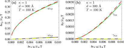
Figure 14: (Color online). Results for an intrinsic double-layer graphene system in the small-$q$ regime with $\kappa=1$, $d=300$ Å and $T=100$ K. (a) Plasmon dispersion versus $\hbar v_{F}q/(k_{B}T)$. (b) Plasmon damping rate versus $\hbar v_{F}q/(k_{B}T)$. The dashed and solid lines correspond to the analytical results (given in Eqs. (22)-(25)) and the numerical results, respectively.

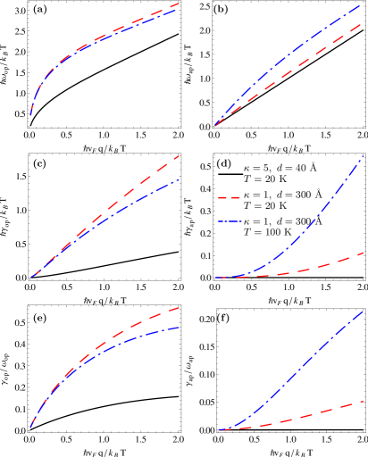
Figure 15: (Color online). Numerical results for an intrinsic double-layer graphene system. (a) and (b) Plasmon dispersion versus $\hbar v_{F}q/(k_{B}T)$; (c) and (d) Plasmon damping rate versus $\hbar v_{F}q/(k_{B}T)$; (e) and (f) $\gamma/\omega_{p}$ versus $\hbar v_{F}q/(k_{B}T)$. (a), (c) and (e) are for the optical plasmon mode. (b), (d) and (f) are for the acoustic plasmon mode. For $\kappa=5$, $d=40$ Å, and $T=20$ K, the acoustic plasmon mode $\omega_{ap}$ is degenerate with the boundary of the single particle excitation region. Note that the legend applies to all sub-figures.

Next, we consider the double-layer graphene plasmons when one layer is doped (“extrinsic”) and one undoped (“intrinsic”), i.e. one layer has carrier density $n\neq 0$ and the other has $n=0$ at $T=0$. The long wavelength and low temperature RPA collective modes of such a mixed intrinsic-extrinsic graphene double-layer system are easily derived to be given by:

$$\omega_{op} = \left[2r_{s}\hbar^{2}v_{F}^{2}qk_{F}\left(1+(2\ln 2)\frac{T}{T_{F}}-\frac{\pi^{2}}{6}\frac{T^{2}}{T^{2}_{F}}\right)\right]^{1/2}$$ (30)

$$\omega_{ap} = \sqrt{(8\ln 2)r_{s}\hbar v_{F}q^{2}dk_{B}T\Big{[}1-\frac{(2\ln 2)T}{T_{F}}+\frac{4(\ln 2)^{2}T^{2}}{T^{2}_{F}}\Big{]}}$$ (31)

$$\gamma_{op} = \left[\frac{\pi^{2}r_{s}^{3}\hbar^{3}v_{F}^{3}q^{3}E_{F}}{128k_{B}^{2}T^{2}}\left(1+(2\ln 2)\frac{T}{T_{F}}-\frac{\pi^{2}}{6}\frac{T^{2}}{T^{2}_{F}}\right)\right]^{1/2}$$ (32)

$$\gamma_{ap} = \sqrt{\frac{\pi^{2}\ln 2r_{s}^{3}\hbar^{3}v_{F}^{3}q^{6}d^{3}}{8k_{B}T}\Big{[}1-(10\ln 2)\frac{T}{T_{F}}+60(\ln 2)^{2}\frac{T^{2}}{T^{2}_{F}}\Big{]}}$$ (33)

Here $r_{s}=e^{2}/(\kappa\hbar v_{F})$ refers to both layers, and $k_{F}=(\pi n)^{1/2}$ and $T_{F}=E_{F}/k_{B}=\hbar v_{F}k_{F}/k_{B}$ refer to the doped extrinsic layer.

While the above results are valid in the $T/T_{F}\ll 1$ (as well as leading order in $q$) limit, we can also obtain the high-temperature ($T/T_{F}\gg 1$) asymptotic analytical results to be exactly the same as those given in Eqs. (22)-(25) for double-layer intrinsic graphene. This is, of course, expected since in the $T\gg T_{F}$ limit, there is no difference in the leading order between intrinsic and extrinsic graphene.

The mixed double-layer intrinsic-extrinsic graphene system depends in a complicated manner on a large number of independent parameters: $q,n,T,d,\kappa$. The plasmon modes now really depend on all five of these parameters (plus the value of $v_{F}$ which in principle is also a free parameter of the theory). We refrain from overloading the readers with a large number of results varying all five parameters freely. We provide some representative plasmon dispersion and damping results in Figs. 16-20 showing the full numerical RPA solutions for the plasmon energy and damping for the mixed double-layer system, emphasizing that our low-temperature (high temperature) analytical results seem to work very well in the $T<T_{F}$ ($T>T_{F}$) regimes, providing an easy and effective way for quick calculations of the plasmon dispersion and damping in double-layer intrinsic-extrinsic plasmon systems. The captions in each figure (in Figs. 16-20) clearly describe in details the parameter values and the numerical results for the mixed intrinsic-extrinsic double layer system.

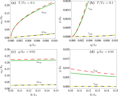
Figure 16: (Color online). Results for a mixed double-layer intrinsic-extrinsic graphene system with $n_{1}=10^{12}$ cm^-2, $n_{2}/n_{1}=0.0$, $d=300$ Å and $\kappa=1$. (a) $\omega_{p}/E_{F}$ versus $q/k_{F}$ for $T/T_{F}=0.1$. (b)$\gamma/E_{F}$ versus $q/k_{F}$ for $T/T_{F}=0.1$. (c) $\omega_{p}/E_{F}$ versus $T/T_{F}$ for $q/k_{F}=0.01$. (d)$\gamma/E_{F}$ versus $T/T_{F}$ for $q/k_{F}=0.01$. The dashed and solid lines correspond to the analytical results (given in Eqs. (30)-(33)) and the numerical results, respectively.

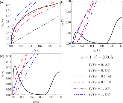
Figure 17: (Color online). Numerical results for a mixed double-layer intrinsic-extrinsic graphene system over a wide $q/k_{F}=0-1$ range with $n_{1}=10^{12}$ cm^-2, $n_{2}/n_{1}=0.0$, $d=300$ Å and $\kappa=1$. (a) $\omega_{p}/E_{F}$ versus $q/k_{F}$ for different temperatures. (b) $\gamma/E_{F}$ versus $q/k_{F}$ for different temperatures. (c) $\gamma/\omega_{p}$ versus $q/k_{F}$ for different temperatures. For $T/T_{F}=0$, the acoustic plasmon mode $\omega_{ap}$ is degenerate with the boundary of the single particle excitation region. Note that the legend applies to all sub-figures.

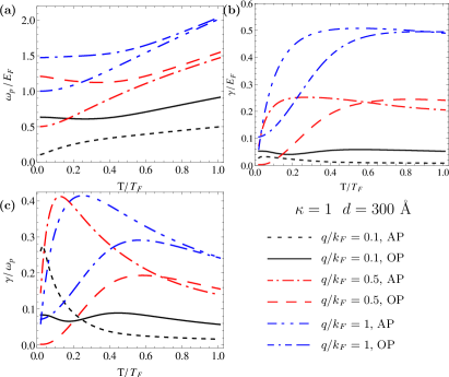
Figure 18: (Color online). Numerical results for a mixed double-layer intrinsic-extrinsic graphene system over a wide $T/T_{F}=0-1$ range with $n_{1}=10^{12}$ cm^-2, $n_{2}/n_{1}=0.0$, $d=300$ Å and $\kappa=1$. (a) $\omega_{p}/E_{F}$ versus $T/T_{F}$ for different $q/k_{F}$. (b) $\gamma/E_{F}$ versus $T/T_{F}$ for different $q/k_{F}$. (c) $\gamma/\omega_{p}$ versus $T/T_{F}$ for different $q/k_{F}$. Note that the legend applies to all sub-figures.

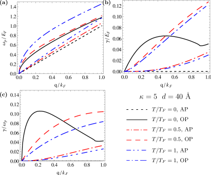
Figure 19: (Color online). Numerical results for a mixed double-layer intrinsic-extrinsic graphene system over a wide $q/k_{F}=0-1$ range with $n_{1}=10^{12}$ cm^-2, $n_{2}/n_{1}=0.0$, $d=40$ Å and $\kappa=5$. (a) $\omega_{p}/E_{F}$ versus $q/k_{F}$ for different temperatures. (b) $\gamma/E_{F}$ versus $q/k_{F}$ for different temperatures. (c) $\gamma/\omega_{p}$ versus $q/k_{F}$ for different temperatures. For $T/T_{F}=0$, the acoustic plasmon mode $\omega_{ap}$ is degenerate with the boundary of the single particle excitation region. Note that the legend applies to all sub-figures.

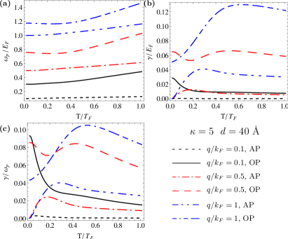
Figure 20: (Color online). Numerical results for a mixed double-layer intrinsic-extrinsic graphene system over a wide $T/T_{F}=0-1$ range with $n_{1}=10^{12}$ cm^-2, $n_{2}/n_{1}=0.0$, $d=40$ Å and $\kappa=5$. (a) $\omega_{p}/E_{F}$ versus $T/T_{F}$ for different $q/k_{F}$. (b) $\gamma/E_{F}$ versus $T/T_{F}$ for different $q/k_{F}$. (c) $\gamma/\omega_{p}$ versus $T/T_{F}$ for different $q/k_{F}$. Note that the legend applies to all sub-figures.

Finally, we conclude this subsection with a brief discussion of the finite-temperature double-layer extrinsic plasmon system when both layers are doped. Since the $T=0$ case for this system was considered in details by Hwang and Das SarmaHwang and Das Sarma (2009) with some follow-up $T\neq 0$ double-layer plasmon calculations in the literatureVazifehshenas et al. (2010); Yuan et al. (2011); Bahrami and Vazifehshenas (2012); Stauber and Gómez-Santos (2012); Stauber and Gomez-Santos (2012); Tuan and Khanh (2012); Profumo et al. (2012); Badalyan and Peeters (2012a, b); Triola and Rossi (2012), we only provide some brief analytical results for the sake of completeness (and comparison with our intrinsic plasmon double layer results). We mention that the extrinsic double-layer plasmons are in principle determined by six independent parameters ($n_{1},n_{2},T,q,d,\kappa$), and providing complete numerical results here will simply make our paper far too long.

Using the asymptotic forms for the graphene polarizability in the long wavelength limit, we get the following analytical formula for the low-temperature ($T\ll T_{F}$) plasmon dispersion and damping in the leading order:

$$\omega_{op} = \sqrt{2r_{s}\hbar^{2}v_{F}^{2}q(k_{F1}+k_{F2})\left(1-\frac{\pi^{2}}{6}\frac{T^{2}}{T_{F1}T_{F2}}\right)}$$ (34)

$$\omega_{ap} = \sqrt{\frac{4r_{s}\hbar^{2}v_{F}^{2}dq^{2}k_{F1}k_{F2}}{k_{F1}+k_{F2}}\frac{(1-\frac{\pi^{2}}{6}\frac{T^{2}}{T^{2}_{F1}})(1-\frac{\pi^{2}}{6}\frac{T^{2}}{T^{2}_{F2}})}{1-\frac{\pi^{2}}{6}\frac{T^{2}}{T_{F1}T_{F2}}}}$$

where $k_{F1,2}=\sqrt{\pi n_{1,2}}$, $k_{B}T_{F1,2}=E_{F1,2}=\hbar v_{F}k_{F1,2}$ depend on the doping carrier density $n_{1,2}$ in the two layers, and $T\ll T_{F1,2}$ is assumed in obtaining Eqs. (34) and (LABEL:eq35:dexana). The corresponding low-temperature long-wavelength damping $\gamma$ for both plasmon modes is exponentially suppressed as in the corresponding single-layer extrinsic plasmon case.

We can also carry out the high-temperature $T\gg T_{F1,2}$ asymptotic expansion of $\Pi_{1,2}$ to derive the corresponding high-temperature results and we get precisely Eqs. (22)-(25) in the leading order in $T_{F1,2}/T$, i.e. $T_{F}$ drops out in the leading order, leaving us precisely the intrinsic double-layer plasmon results, as expected. The precise agreement between the extrinsic and the intrinsic results arises in the leading order in $T_{F}/T$ because the finite-$T$ chemical potential in the extrinsic case goes as $\mu\approx\frac{E_{f}}{4\ln 2}\frac{T_{F}}{T}$ for $T_{F}\ll T$.

We just show three representative sets of numerical results for double-layer extrinsic graphene in Figs. 21-23. In Fig. 21, the small-$q$ and small-$T$ numerical results are shown manifesting excellent agreement with our $T\ll T_{F}$ analytical results. In Fig. 22 we show the results for the same parameters in a much more expanded scale of $q/k_{F1}$. In Fig. 23 we show the temperature dependence at fixed $q$.

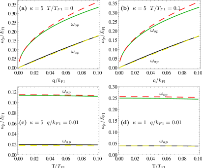
Figure 21: (Color online). Results for a double-layer extrinsic graphene system with $n_{1}=10^{12}$ cm^-2, $n_{2}/n_{1}=0.25$, $d=300$ Å. (a) and (b) $\omega_{p}/E_{F1}$ versus $q/k_{F1}$. (c) and (d) $\omega_{p}/E_{F1}$ versus $T/T_{F1}$. The dashed and solid lines correspond to the analytical results (given in Eqs. (34)-(LABEL:eq35:dexana)) and the numerical results, respectively.

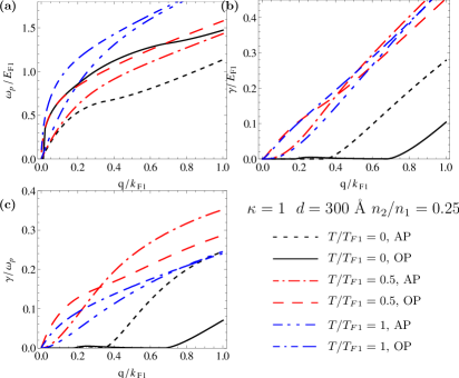
Figure 22: (Color online). Results for a double-layer extrinsic graphene system with $n_{1}=10^{12}$ cm^-2, $n_{2}/n_{1}=0.25$, $d=300$ Å and $\kappa=1$. (a) $\omega_{p}/E_{F1}$ versus $q/k_{F1}$ for different temperatures. (b) $\gamma/E_{F1}$ versus $q/k_{F1}$ for different temperatures. (c) $\gamma/\omega_{p}$ versus $q/k_{F1}$ for different temperatures. Note that the legend applies to all sub-figures.

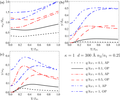
Figure 23: (Color online). Results for a double-layer extrinsic graphene system with $n_{1}=10^{12}$ cm^-2, $n_{2}/n_{1}=0.25$, $d=300$ Å and $\kappa=1$. (a) $\omega_{p}/E_{F1}$ versus $T/T_{F1}$ for different $q/k_{F1}$. (b) $\gamma/E_{F1}$ versus $T/T_{F1}$ for different $q/k_{F1}$. (c) $\gamma/\omega_{p}$ versus $T/T_{F1}$ for different $q/k_{F1}$. Note that the legend applies to all sub-figures.

II.3 Bilayer graphene

Finally, we very briefly consider the theory for intrinsic plasmons in undoped bilayer graphene (BLG) for the sake of completeness. For our purpose, we assume the bilayer graphene to have parabolic chiral band structureWang and Chakraborty (2007); Borghi et al. (2009); Sensarma et al. (2010); Wang and Chakraborty (2010); Gamayun (2011) (characterized by an effective mass $m$ rather than a velocity $v_{F}$) in contrast to the linear chiral band structure of MLG (which is what we have considered so far in this work).

The BLG 2D polarizability function is given bySensarma et al. (2010):

$$\Pi(q,\omega)=-\frac{4}{L^{2}}\underset{\mathbf{k},s,s^{\prime}}{\sum}\frac{f_{s,\mathbf{k}}-f_{s^{\prime},\mathbf{k^{\prime}}}}{\hbar\omega+\epsilon_{s,\mathbf{k}}-\epsilon_{s^{\prime},\mathbf{k^{\prime}}}+i\eta}F_{s,s^{\prime}}(\mathbf{k},\mathbf{k^{\prime}})$$ (36)

where $\mathbf{k^{\prime}=k+q}$, $s,s^{\prime}=\pm 1$, $\epsilon_{s,\mathbf{k}}=s\hbar^{2}\mathbf{k}^{2}/(2m)$ and $F_{s,s^{\prime}}=(1+\cos 2\theta)/2$ is the chiral wavefunction overlap. The functions “$f$” in Eq. (36) are the Fermi distribution functions at temperature $T$. The bilayer dynamical polarizability first calculated by Sensarma et al.Sensarma et al. (2010) who also first obtained the bilayer graphene plasmon dispersion for the extrinsic (doped) system. Blow we give the analytical results for intrinsic BLG plasmons in the absence of any doping.

In the long wavelength limit ($q\rightarrow 0$) and at high temperatures $\hbar^{2}q^{2}/(2m)\ll k_{B}T$, we have the following asymptotic formula for BLG $\Pi(q,\omega)$ in the intrinsic ($n=0$) regime (from a direct expansion of Eq. (36) above):

$$\Pi(q,\omega)\approx\frac{4\ln 2}{\pi}\frac{q^{2}}{\omega^{2}}k_{B}T+i\frac{q^{2}}{8k_{B}T}$$ (37)

Using Eq. (1) for the plasmon oscillation, we get the mode dispersion and damping for intrinsic BLG to be:

$$\omega_{p} = \sqrt{\frac{8e^{2}(\ln 2)(k_{B}T)q}{\kappa}}$$ (38)

$$\gamma = \frac{\pi e^{2}q}{2\kappa\sqrt{2\kappa k_{B}T}}\sqrt{(\ln 2)e^{2}q}$$ (39)

This gives for the BLG intrinsic plasmon:

$$\omega_{p}/\gamma=\frac{8k_{B}T\kappa}{\pi e^{2}q}$$ (40)

For well-defined modes, we must have $\omega_{p}/\gamma>1$, leading to the condition that:

$$k_{B}T>\frac{\pi e^{2}q}{8\kappa}$$ (41)

Thus, similar to the MLG intrinsic plasmon although $\gamma\propto 1/\sqrt{T}$, there is a well-defined intrinsic plasma mode at long wavelength for arbitrarily low temperatures.

Comparing the BLG intrinsic plasmon dispersion given in Eq. (38) with the corresponding MLG expression given in Eq. (7), we see that the MLG and the BLG results are identical except for an extra factor of $2$ ($8\ln 2$ in Eq. (38) and $4\ln 2$ in Eq. (7)) in the BLG case. (Remember that $r_{s}=e^{2}/(\kappa\hbar v_{F})$ making Eq. (7) equivalent to $\omega_{p}=\sqrt{(4\ln 2)e^{2}k_{B}Tq/\kappa}.$) Thus the intrinsic plasmon frequency, in sharp contrast to the extrinsic plasmon frequency, is independent of the Fermi velocity (MLG) or the effective mass (BLG) and depends only on a single material constant $\kappa$, the background dielectric constant. We note that the expressions for the intrinsic plasmon damping is also very similar for MLG (Eq. (8)) and BLG (Eq. (40))—again except for a factor of $\sqrt{8}$, the two expressions are identical (and independent of $v_{F}$ or $m$).

We can also obtain the analytical results for the intrinsic plasmons in the double-layer BLG system composed of two BLG layers separated by a distance “$d$”. Solving the $2\times 2$ determinantal equation (Eq. (18)) for the double-layer BLG system, we get the following analytic leading-order results for the intrinsic plasmons of the double-layer BLG system:

$$\omega_{op} = \sqrt{(16\ln 2)qk_{B}T\frac{e^{2}}{\kappa}}$$ (42)

$$\omega_{ap} = \sqrt{(8\ln 2)q^{2}dk_{B}T\frac{e^{2}}{\kappa}}$$ (43)

$$\gamma_{op} = \frac{\pi qe^{2}}{\kappa\sqrt{k_{B}T}}\sqrt{(\ln 2)\frac{e^{2}}{\kappa}q}$$ (44)

$$\gamma_{ap} = \frac{\pi q^{2}de^{2}}{2\kappa\sqrt{2k_{B}T}}\sqrt{(\ln 2)q^{2}d\frac{e^{2}}{\kappa}}$$ (45)

These formula for the intrinsic double-layer BLG plasmons are essentially identical to the corresponding double-layer MLG intrinsic plasmons (Eqs.(22)-(25)) except for numerical factors. Again, these plasmon mode dispersion and damping do not depend on the effective mass or the Fermi velocity and are universal properties of the intrinsic system.

III Discussion

Given the very large number of systems considered in this work (MLG, BLG, intrinsic, extrinsic, single layer, double-layer, $\cdots$) and the numerous analytical (as well as numerical) results presented in Sec.II, it is useful to summarize all the analytical results in Tables 1 and 2 so that the similarities/differences/connections among the various derived results for plasmon modes (and their damping) become apparent. Some of the results in Tables 1 and 2 were obtained in the literature before, but our emphasis in this work is on intrinsic plasmon modes and their temperature dependence. Results in the last row of Tables 1 and 2 are for the ordinary (non-chiral) 2D electron gas systems (as occurring, for example, in semiconductor quantum wells) , which are by definition extrinsic systems since the large band gap (between conduction and valence bands) in the semiconductor ensures that for $n=0$, there is no plasmon mode in the system.

The key issue to be discussed in this section is the feasibility of an experimental observation of the graphene intrinsic Dirac point plasmon, which will be the manifestation of a qualitatively new phenomenon since such intrinsic plasmons at zero doping density in a charge neutral system is essentially impossible in any 2D (or 3D) semiconductors where the existence of free carriers necessitates doping by some means. (As an aside we mention that even in a very narrow gap semiconductor, e.g. In As or InSb, the band gap is $\gtrsim 100$ meV, which implies that $T>2000$ K is necessary for any appreciable thermal population of free carriers making it impossible to study any kind of “intrinsic plasmons” in undoped semiconductors.)

There has been a great deal of recent experimental interest in studying the properties of graphene Dirac point (i.e. the charge neutrality point) in both MLG and BLG systemsWeitz et al. (2010); Ponomarenko et al. (2011); Jr et al. (2012); Bao et al. (2012). Various exotic quantum phases Min et al. (2008); Barlas and Yang (2009); Zhang et al. (2010); Lemonik et al. (2010); Nandkishore and Levitov (2010a, b, c); Vafek and Yang (2010); Jung et al. (2011) and non-Fermi liquid behaviorDas Sarma et al. (2007) are theoretically predicted at the graphene Dirac point, and thus the possibility of understanding the Dirac point behavior through the observation of intrinsic plasmon properties is both interesting and intriguing. For example, our theory of intrinsic Dirac point plasmon modes developed in this work is based entirely on the random phase approximation assuming a generic Fermi liquid ground state, and consequently, any observed qualitative departure in the experimentally observed Dirac point plasmon behavior (e.g. a completely different temperature dependence compared with that given in Tables. 1 and 2) would imply a failure of RPA indicating the fundamental and qualitative importance of interaction effects or perhaps even the emergence of a new spontaneously symmetry-broken ground state as has been predicted theoretically in the literatureHerbut (2006); Nomura and MacDonald (2006); Yang et al. (2006); Drut and Lähde (2009a); Neto et al. (2009); Lemonik et al. (2012); Kotov et al. (2012). Since collective modes (e.g. Goldstone modes, Higgs bosons, zero sound modes, etc.) typically tell us a great deal about the fundamental nature of the field theoretic vacuum (i.e. the ground state of the system), the study of graphene intrinsic plasmons could turn out to be a very useful route to understanding the nature of the Dirac point. A good example of the possible usefulness of intrinsic plasmons could be in the determination of whether the nonperturbative aspects of electron-electron interaction induce a chiral anomaly in graphene leading to the spontaneous formation of an energy gap at the Dirac point as has been predicted in some lattice quantum Monte Carlo simulationDrut and Lähde (2009b); Drut and Lähde (2009c, a). Such an energy gap at the Dirac point, if it exists in the experimental samples, would show up as an exponential (going as $e^{-\Delta/T}$ where $\Delta$ is the induced gap) suppression of the intrinsic plasmon energy (i.e. the simple power laws in temperature derived in our RPA theory will fail qualitatively), which could be directly experimentally observed thus validating (or not) the existence of a Dirac point chiral anomaly.

Material	System		High Temperature $T\rightarrow\infty$
			$\omega_{p}$	$\gamma$	Comments
MLG	Intrinsic		$\omega_{pi}$	$\gamma_{pi}$
	Extrinsic		$\omega_{pi}\sqrt{1+\frac{{T_{F}}^{4}}{128(\ln 2)^{3}T^{4}}}$	$\gamma_{pi}\left[1-\frac{(\ln 2)e^{2}q}{12\kappa k_{B}T}\right]$
Double MLG	Two Intrinsic	OP	$\sqrt{2}\omega_{pi}$	$\sqrt{8}\gamma_{pi}$
		AP	$\sqrt{qd}\ \omega_{pi}$	$(qd)^{\frac{3}{2}}\ \gamma_{pi}$
	Intrinsic-Extrinsic	OP	Same as results for double intrinsic layers		For $T\rightarrow\infty$, chemical potential of MLG $\mu\rightarrow 0$
		AP
	Two Extrinsic	OP
		AP
BLG	Intrinsic		$\sqrt{2}\omega_{pi}$	$\sqrt{8}\gamma_{pi}$
	Extrinsic		$\sqrt{2+\frac{T_{F}^{2}}{(4\ln 2)T^{2}}}\omega_{pi}$	$\sqrt{8}\Big{[}1-\frac{8\ln 2-2}{32\ln 2}\frac{T_{F}^{2}}{T^{2}}\Big{]}\gamma_{pi}$
Double BLG	Two Intrinsic	OP	$2\omega_{pi}$	$8\gamma_{pi}$
		AP	$\sqrt{2qd}\omega_{pi}$	$\sqrt{8}(qd)^{\frac{3}{2}}\ \gamma_{pi}$
	Intrinsic-Extrinsic	OP	Same as results for double intrinsic layers		For $T\rightarrow\infty$, $T_{F}/T\rightarrow 0$
		AP
	Two Extrinsic	OP
		AP
2DEG	Single layer		$\sqrt{\frac{2\pi ne^{2}q}{m\kappa}}[1+\frac{3}{4}\frac{q\kappa k_{B}T}{\pi e^{2}n}]$	$\sqrt{\frac{\pi}{k_{B}T}}\left(\frac{\pi e^{2}n}{\kappa q}\right)^{\frac{3}{2}}\text{exp}\left[-\frac{\pi e^{2}n}{\kappa k_{B}Tq}-\frac{3}{2}\right]$
	Double layer1	OP	$\sqrt{\frac{2\pi e^{2}q(n_{1}+n_{2})}{m\kappa}}$	$\sqrt{\frac{\pi(n_{1}+n_{2})}{k_{B}T}}\left(\frac{\pi e^{2}}{\kappa q}\right)^{\frac{3}{2}}\Big{[}e^{-\frac{\pi e^{2}n_{1}}{\kappa k_{B}Tq}-\frac{3}{2}}n_{1}+e^{-\frac{\pi e^{2}n_{2}}{\kappa k_{B}Tq}-\frac{3}{2}}n_{2}\Big{]}$
		AP	$\sqrt{\frac{4\pi e^{2}q^{2}d}{m\kappa}}\sqrt{\frac{n_{1}n_{2}}{n_{1}+n_{2}}}$	$\sqrt{\frac{\pi}{k_{B}T}}\left(\frac{2\pi e^{2}}{\kappa}\frac{dn_{1}n_{2}}{n_{1}+n_{2}}\right)^{\frac{3}{2}}\frac{\text{exp}[-\frac{\pi e^{2}n_{2}}{\kappa k_{B}Tq}-\frac{3}{2}]n_{1}+\text{exp}[-\frac{\pi e^{2}n_{1}}{\kappa k_{B}Tq}-\frac{3}{2}]n_{2}}{n_{1}+n_{2}}$

Table 1: Summary of high temperature analytical results. We denote $\omega_{pi}=\sqrt{\frac{4(\ln 2)(k_{B}T)e^{2}q}{\kappa}}$, $\gamma_{pi}=\frac{\pi}{8}\sqrt{\frac{\ln 2}{k_{B}T}}\Big{(}\frac{e^{2}q}{\kappa}\Big{)}^{\frac{3}{2}}$. Note 1: only the leading order terms are kept in obtaining results for a double-layer two-dimensional electron gas (2DEG) system.

Material	System		Low Temperature $T\rightarrow 0$
			$\omega_{p}$	$\gamma$	Comments
MLG	Intrinsic		N/A	N/A	No plasmon mode at $T=0$
	Extrinsic		$\omega_{px1}\sqrt{\Big{[}1-\frac{\pi^{2}}{6}\frac{T^{2}}{T_{F}^{2}}\Big{]}}$	N/A	$\gamma$ exponentially suppressed
Double MLG	Two Intrinsic	OP	N/A		No plasmon mode at $T=0$
		AP
	Intrinsic-Extrinsic1	OP	$\omega_{px1}\sqrt{1+(2\ln 2)\frac{T}{T_{F1}}-\frac{\pi^{2}}{6}\frac{T^{2}}{T^{2}_{F1}}}$	$\gamma_{pi}\sqrt{\frac{T_{F1}}{(2\ln 2)T}+1-\frac{\pi^{2}}{12\ln 2}\frac{T}{T_{F1}}]}$
		AP	$\omega_{pi}\sqrt{2qd\Big{[}1-(2\ln 2)\frac{T}{T_{F1}}+4(\ln 2)^{2}\frac{T^{2}}{T^{2}_{F1}}\Big{]}}$	$\gamma_{pi}\sqrt{8(qd)^{3}[1-\frac{(10\ln 2)T}{T_{F1}}]}$
	Two Extrinsic	OP	$\sqrt{(\omega_{px1}^{2}+\omega_{px2}^{2})\Big{[}1-\frac{\pi^{2}}{6}\frac{T^{2}}{T_{F1}T_{F2}}\Big{]}}$	N/A	$\gamma$ exponentially suppressed
		AP	$\sqrt{2qd\omega_{px1}\omega_{px2}\frac{\sqrt{k_{F1}k_{F2}}}{k_{F1}+k_{F2}}}\sqrt{\frac{(1-\frac{\pi^{2}}{6}\frac{T^{2}}{T^{2}_{F1}})(1-\frac{\pi^{2}}{6}\frac{T^{2}}{T^{2}_{F2}})}{1-\frac{\pi^{2}}{6}\frac{T^{2}}{T_{F1}T_{F2}}}}$
BLG	Intrinsic		N/A		No plasmon
	Extrinsic		$\sqrt{\frac{2\pi ne^{2}q}{m\kappa}}$	N/A	$\gamma$ exponentially suppressed
Double BLG	Two Intrinsic	OP	N/A		No plasmon mode
		AP
	Intrinsic-Extrinsic1	OP	$\sqrt{\frac{2\pi e^{2}qn}{m\kappa}}\sqrt{1+2\ln 2\frac{T}{T_{F1}}}$	$\gamma_{pi}\sqrt{\frac{4T_{F1}}{(\ln 2)T}}$
		AP	$\omega_{pi}\sqrt{4qd\Big{[}1-(2\ln 2)\frac{T}{T_{F1}}\Big{]}}$	$8(qd)^{\frac{3}{2}}\gamma_{pi}$
	Two Extrinsic	OP	$\sqrt{\frac{2\pi e^{2}q(n_{1}+n_{2})}{m\kappa}}$	N/A	$\gamma$ exponentially suppressed
		AP	$\sqrt{\frac{4\pi e^{2}q^{2}d}{m\kappa}}\sqrt{\frac{n_{1}n_{2}}{n_{1}+n_{2}}}$
2DEG	Single layer		$\sqrt{\frac{2\pi ne^{2}q}{m\kappa}}$	N/A	$\gamma$ exponentially suppressed
	Double layer	OP	$\sqrt{\frac{2\pi e^{2}q(n_{1}+n_{2})}{m\kappa}}$	N/A	$\gamma$ exponentially suppressed
		AP	$\sqrt{\frac{4\pi e^{2}q^{2}d}{m\kappa}}\sqrt{\frac{n_{1}n_{2}}{n_{1}+n_{2}}}$

Table 2: Summary of low temperature analytical results. We denote $\omega_{px1}=\sqrt{2\frac{e^{2}\sqrt{\pi n_{1}}\hbar v_{F}q}{\kappa}}$, $\omega_{px2}=\sqrt{2\frac{e^{2}\sqrt{\pi n_{2}}\hbar v_{F}q}{\kappa}}$, $\omega_{pi}=\sqrt{\frac{4(\ln 2)(k_{B}T)e^{2}q}{\kappa}}$, and $\gamma_{pi}=\frac{\pi}{8}\sqrt{\frac{\ln 2}{k_{B}T}}\Big{(}\frac{e^{2}q}{\kappa}\Big{)}^{\frac{3}{2}}$. Note 1: results for a mixed intrinsic-extrinsic graphene double-layer system are obtained in the limit $\hbar v_{F}q\ll k_{B}T\ll E_{F1}$. For $k_{B}T\ll\hbar v_{F}q$, there is only an optical plamson mode $\omega_{op}$, determined by the extrinsic layer, in a mixed double-layer graphene system.

Thus, an experimental investigation of intrinsic Dirac plasmons is highly desirable. It may appear to be a straightforward, even a trivial, task to study intrinsic Dirac plasmons experimentally by carrying out plasmon experiments keeping the Fermi level fixed at the charge neutrality point by appropriately tuning the gate voltage in gated graphene. Transport measurements in gated samples routinely enable sitting precisely at the charge neutrality point since the graphene conductivity has a typical “V” or “U” shape as a function of gate voltage with the conductivity (resistivity) minimum (maximum) being located at the nominal Dirac point. The serious complication is, however, disorder since it is well-knownDas Sarma et al. (2011); Adam et al. (2007); Rossi and Das Sarma (2008); Martin et al. (2008); Zhang et al. (2009); Deshpande et al. (2009, 2011) that the charge neutrality point as determined by transport or other experiments is not the theoretical Dirac point because of the existence of electron-hole puddles in the system. In particular, random charged impurities in the graphene environment become qualitatively important in the $n\lesssim n_{i}$ regime (where $n_{i}$ is the impurity density and $n$ the carrier density), and drive the system into a highly inhomogeneous state with randomly distributed puddles of electrons and holes dominating the landscape. This puddle-dominated highly inhomogeneous (i.e. carrier density fluctuates spatially) regime has been shownAdam et al. (2007); Rossi et al. (2009); Das Sarma et al. (2011); Li et al. (2011) to correspond to the so-called minimum conductivity plateau in the graphene transport data (i.e. the bottom of the “V” or “U” in the conductivity versus gate voltage plot). Thus, the charge neutrality point in transport corresponds only to the total charge density in the whole sample being zero, and not to the absence of electrons and holes in the system. The puddle-dominated regime around the charge neutrality point should be best thought of as a random spatial variation in the Dirac point with respect to the spatially constant chemical potential (as controlled by the external gate voltage) where at each point in space the Dirac point is either above (“hole regions”) or below (“electron regions”) the chemical potential. Within the mean field theoryAdam et al. (2007); Rossi et al. (2009); Das Sarma et al. (2011); Li et al. (2011); Das Sarma et al. (2012); Das Sarma and Hwang (2013) the system has a finite fluctuation induced carrier density ($n^{*}\sim n_{i}$) even at the Dirac point (i.e. the charge neutrality point) because of the Coulomb disorder induced electron-hole puddles.

The existence of electron-hole puddles means that the Dirac point is ill-defined experimentally upto a carrier density of $n^{*}$ (with $n^{*}$ being determined by the details of the random charged impurity configuration in the system, but typically $n^{*}\lesssim n_{i}$), and $n^{*}$ can be approximately estimated experimentally by looking at the size of the conductivity minimum plateau regionChen et al. (2008). The lack of the precise existence of the Dirac point has obvious implications for the intrinsic plasmon which we discuss below.

Electron-hole puddles make it impossible, as a matter of practice, to explore the precise Dirac point in graphene (or other similar materials), and therefore, our assumption of $n\equiv 0$ at the Dirac point is no longer applicable in our consideration of intrinsic plasmons. This, however, should not be construed as a complete disaster for the observation of the intrinsic plasmon since the Dirac point, being a set of measure zero, would naturally be difficult to approach in any experimentDas Sarma and Hwang (2013), and all experimental claims of studying Dirac point phenomena are suspect because of the fragile and unstable nature of this “measure-zero” fixed point. Any experimental technique requiring the precise placement of the Fermi level at the Dirac point (i.e. $n\equiv 0$ everywhere in the sample) is doomed to fail no matter what.

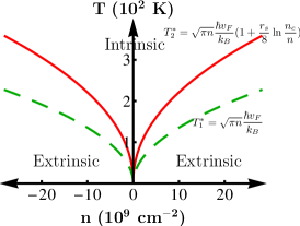
Figure 24: (Color online). The temperature scale for the crossover of the collective mode from being intrinsic to being extrinsic. The dashed curve shows $T_{1}^{*}(n)=\sqrt{\pi n}\hbar v_{F}/k_{B}$. The solid curve shows $T_{2}^{*}(n)=\sqrt{\pi n}\frac{\hbar v_{F}}{k_{B}}(1+\frac{r_{s}}{8}\ln\frac{n_{c}}{n})$ including Fermi velocity renormalization due to electron-electron interactions (see Ref. [Hwang et al., 2007] for details), where $r_{s}=0.4$ ($\kappa=5$) and $n_{c}=10^{15}$ cm^-2 is the high density cut off.

From our presented results in Sec. II (see also Tables 1 and 2), it is rather obvious that for the physics of intrinsic plasmons to manifest itself experimentally, there would be a lower cut-off ($T^{*}$) in the temperature below which (i.e. for $T<T^{*}$) the electron-hole puddles would inhibit any observation of intrinsic plasmon behavior with the collective mode basically crossing over from being intrinsic for $T\gg T^{*}$ to being extrinsic for $T\ll T^{*}$. Clearly, the temperature scale for this crossover is given by

$$T^{*}=T_{F}(n^{*})=\hbar v_{F}\sqrt{\pi n^{*}}/k_{B}$$ (46)

where $n^{*}$ is the average puddle-induced carrier density in the system (i.e. $n^{*}$ is a function of $n_{i}$). Thus, intrinsic Dirac point behavior is essentially a high-temperature phenomenon with the intrinsic plasmon manifesting itself only for $T\gg T^{*}$ and then crossing over to extrinsic plasmons of the puddle carriers for $T\ll T^{*}$. The fact that the intrinsic Dirac point behavior is an effective “high-temperature” behavior has already been emphasized earlier in the context of approaching the Dirac point through transport measurementsDas Sarma and Hwang (2013), and in the current work, we establish the same qualitative finding for approaching the Dirac point through collective mode properties. In Fig. 24, we show two possible crossover behaviors between intrinsic and extrinsic plasmons around the Dirac point with intrinsic plasmon being always the “high-temperature” mode appearing in the quantum critical “fan” region and extrinsic plasmon dominating the non-critical low-temperature and high-density region.

In standard graphene on SiO₂ substrates, with substantial impurity content in the environment, the typical puddle-induced carrier density $n^{*}\sim 10^{12}$ cm^-2, which gives $T^{*}\sim 1500$ K, and obviously it makes no sense to discuss any experimental study of intrinsic plasmons in such “impure” graphene samples because the required temperature scale is impractically high. One can, of course, study extrinsic graphene in such samples by creating a doped carrier density $n>n^{*}$, and induced extrinsic graphene plasmons have been studied in such disordered samples at high carrier densityFei et al. (2011); Chen et al. (2012); Fei et al. (2012). In suspended grapheneBolotin et al. (2008) or graphene on h-BN substratesDean et al. (2010), however, the environmental charged impurity density is very low ($n_{i}<10^{9}$ cm^-2), and very low $n^{*}$ ($\sim 10^{9}-10^{8}$ cm^-2) has been reported with very sharp and narrow conductivity minimum at the charge neutrality point. Such ultrapure graphene samples (with typical mobility $\mu_{m}>100,000$ cm²/V$\cdot$S) with very low puddle density are the appropriate samples for studying intrinsic graphene. For $n^{*}=10^{9}(10^{8})$ cm^-2, $T_{F}\approx 50$ K ($15$ K), and then the necessary condition ($T\gg T^{*}$) for the manifestation of intrinsic plasmon collective behavior would necessitate $T\approx 20-100$ K, which is very reasonable from an experimental perspective. We have already emphasized in Section II (and this is apparent in Tables 1 and 2) that the extrinsic plasmon behaves precisely as an intrinsic plasmon (i.e. $\omega_{p}\propto\sqrt{T}$ and a broadening $\gamma\propto 1/\sqrt{T}$) for $T\gg T_{F}$, which then crosses over to the temperature-independent plasma frequency and exponentially suppressed broadening, the characteristic features of extrinsic plasmon, at low temperatures $T\ll T_{F}$. This is what we would expect for high-quality graphene samples ($n^{*}\sim 10^{8}-10^{9}$ cm^-2) at the Dirac point with respect to their plasmon properties. The plasmon properties will behave like those shown in Fig. 9 at higher temperatures ($T\gg T^{*}\sim 10-50$ K) to those shown in Fig. 1 at lower temperatures ($T\ll T^{*}\sim 10-50$ K). Such an observation will be a direct manifestation of intrinsic Dirac point behavior.

Before concluding this section, we comment on the expected plasmon level broadening (or damping) as manifested by the line width of the experimental plasmon peak. Our calculated damping ($\gamma$) corresponds to the inherent Landau damping induced level broadening which changes the plasmon peak from a pure delta-function like pole in the response function to an approximate broadened Lorentzian shape:

$$\delta(\omega-\omega_{p})\rightarrow\frac{\Gamma}{(\omega-\omega_{p})^{2}+\Gamma^{2}}$$ (47)

The broadening $\Gamma$ in the Lorentzian plasmon peak in Eq. (47) would, in general, have two contributions, arising from Landau damping ($\gamma$) and impurity broadening ($\gamma_{t}$) which can be written as $\gamma_{t}=\hbar/(2\tau)$ where $\tau$ is the transport relaxation time for impurity scattering as extracted from the mobility. In the leading order, we can simply use:

$$\Gamma=\gamma+\gamma_{t}$$ (48)

where $\gamma$ is the Landau damping calculated in Sec. II (see e.g., Tables 1 and 2) and $\gamma_{t}$ is the impurity-scattering induced level broadening which is given by:

$$\gamma_{t}=\hbar/(2\tau_{t})$$ (49)

For high mobility samples $\tau_{t}\propto\mu_{m}$ is very large, and $\gamma_{t}\propto\mu_{m}^{-1}$ is small. Such a small impurity induced broadening will also be necessary for an unambiguous identification of the intrinsic plasmon — it is not enough to just have small values of only the intrinsic Landau damping $\gamma$. Fortunately, the necessary condition for the suppression of $n^{*}$ and $T^{*}$ (i.e. the suppression of puddles) also necessitates very large (small) values of $\tau_{t}(\gamma_{t})$ since low impurity density ($n_{i}\sim n^{*}$) implies high mobility (since $\mu_{m}\sim 1/n_{i}$) and low $\tau_{t}$. Thus, very high-mobility samples with very low puddle density, ensuring both $\gamma_{t}$ and $n^{*}$ to be small, would be necessary for the experimental study of intrinsic plasmons. Fortunately, such high-quality samples already exist in the laboratoryPonomarenko et al. (2011), where the background impurity density ($n_{i}$) is very low, thus ensuring that both $T^{*}$ and $\gamma_{t}$ are low enough for the experimental investigation of intrinsic plasmons.

IV Conclusion

We have provided a rather comprehensive theory for the intrinsic collective plasmon modes in graphene associated with the Dirac point within the dynamical finite-temperature random phase approximation. We have considered monolayer graphene, bilayer graphene and double-layer graphene (consisting of two MLG or BLG layers parallel to each other separated by a distance in the third direction). We have obtained within RPA extensive analytical results for both plasmon dispersion and damping in the experimentally relevant long wavelength limit, and have provided detailed numerical results valid for arbitrary wavevectors and temperatures. We have critically discussed the experimental feasibility for observing the graphene intrinsic plasmon modes.

Among our more important qualitative conclusions (arising from the theory developed in this paper) are: (i) although the intrinsic plasmon modes, being inherently finite-temperature excitations, are strongly Landau damped even at low temperatures, they remain well-defined in the sense that the energy of the mode is larger than its damping in a very large regime of temperature, wavevector, and background dielectric constant; (ii) the intrinsic plasmon is inherently a “high-temperature” phenomenon since the Dirac point has no energy scale (and thus any finite temperature, no matter how low, is inherently a high temperature); (iii) closely connected with the last item is the corollary that the best experimental approach toward the observation of the intrinsic plasmon is to study low-density extrinsic plasmon at temperatures high enough (i.e. $T\gg T_{F}$ so that the effect of doping density is minimal); (iv) high-quality currently available graphene samples (either suspended graphene or graphene on h-BN substrates) with very high mobility should manifest clear-cut evidence for the intrinsic plasmon (e.g. plasmon energy increasing as $\sqrt{T}$ and plasmon damping decreasing as $\sqrt{T}$ with increasing temperature) if experiments are carried out at $T\approx 100$ K with the gate voltage tuned to the nominal charge neutrality point; (v) the collective mode dispersion and damping for intrinsic MLG and BLG plasmons is essentially identical (with $\omega_{p}\propto\sqrt{qT}$ and $\gamma\propto q\sqrt{qT}$ in both) except for numerical factors); (vi) our theoretically calculated analytical formula for plasmon dispersion and damping (both for intrinsic and for extrinsic plasmons) seem to agree with the full RPA numerical results essentially at all wavevectors and temperatures as long as our low-temperature analytical formula is used for $T\lesssim T_{F}$ and the high-temperature analytical formula is used for $T\gtrsim T_{F}$ for extrinsic graphene; (vii) for double-layer systems, we establish that it should be experimentally possible to observe both the optical and the acoustic intrinsic plasmon.

Before concluding, we mention that the graphene plasmon frequency is likely to be affected by interaction effects even at long wavelength, unlike the long-wavelength plasma frequency in parabolic band systems which is protected by Galilean invariance and the associated $f$-sum rule so that only the band mass enters the definition of the long-wavelength plasma frequency, since graphene energy dispersion obeys Lorentz invariance. We believe that RPA is still an excellent approximation for the graphene plasmon properties (since RPA accounts for the long-range Coulomb potential correctly and nonperturbatively) except perhaps that the velocity entering the expression for the graphene plasmon mode should be modified to be the renormalized graphene velocity due to electron-electron interaction as calculated for example in Ref. [Das Sarma et al., 2007]. This simple modification, plus possibly some quantum critical correction arising from the Dirac point which has to be calculated from the renormalization group flow well beyond the scope of our RPA theory, in the spirit of Landau Fermi liquid theory should suffice to incorporate the leading order interaction effect in the plasma frequency since the $r_{s}$ values characterizing Coulomb interaction strength in graphene are typically not too large. A more detailed theory for including interaction effects in the graphene plasmon properties is well beyond the scope of our work and would require substantial future theoretical efforts.

We now conclude by discussing one important point which follows directly from our theoretical work with implications for graphene plasmonics. The recent interest in graphene plasmonics arises from the fact that graphene is a nanostructure allowing for very tight size confinementWang et al. (2011) and that the graphene (extrinsic) plasmon has energy tunable by gate voltage (i.e. $\omega_{p}\sim q^{1/2}n^{1/4}$) through the carrier density. In the case of intrinsic plasmon, however, the plasma energy goes as $\omega_{p}\sim q^{1/2}T^{1/2}$ since basically the doping density $n$ in the extrinsic formula gets replaced by the thermal electron-hole excitation density (i.e. $n\sim T^{2}$). This implies that it should be relatively easy to tune the intrinsic plasmon energy simply by changing temperature while sitting at the charge neutrality point,. Since the temperature dependence ($\sim\sqrt{T}$) of the intrinsic plasmon frequency is much stronger than the doping density dependence (i.e. $n^{1/4}$) of the extrinsic plasmon frequency, it may be more convenient to use the thermal tuning of the plasma frequency than the gate voltage tuning considered so far. In addition, the intrinsic plasmon should be a relatively strong and well-defined mode at room temperatures ($T\sim 300$ K) in high-mobility graphene samples, making it an interesting candidate for possible plasmonic applications.