The response of reduced models of multiscale dynamics to small external perturbations

Abstract

In real-world geophysical applications (such as predicting the climate change), the reduced models of real-world complex multiscale dynamics are used to predict the response of the actual multiscale climate to changes in various global atmospheric and oceanic parameters. However, while a reduced model may be adjusted to match a particular dynamical regime of a multiscale process, it is unclear why it should respond to external perturbations in the same way as the underlying multiscale process itself. In the current work, the authors study the statistical behavior of a reduced model of the linearly coupled multiscale Lorenz 96 system in the vicinity of a chosen dynamical regime by perturbing the reduced model via a set of forcing parameters and observing the response of the reduced model to these external perturbations. Comparisons are made to the response of the underlying multiscale dynamics to the same set of perturbations. Additionally, practical viability of linear response approximation via the Fluctuation-Dissipation theorem is studied for the reduced model.

1 Introduction

A reduced model for slow variables of multiscale dynamics is a lower-dimensional dynamical system, which “resolves” (that is, qualitatively approximates in some appropriate sense) major large scale slow variables of the underlying higher-dimensional multiscale dynamics while at the same time being relatively simple and computationally inexpensive to work with. This is important in real-world applications of contemporary science, such as geophysical science and climate change prediction [19, 21, 15, 37, 14, 28, 24], where the actual underlying physical process is impossible to model directly, and its reduced approximation has to be designed for such a purpose. Reduced dynamics were used to model global circulation patterns [18, 13, 36, 48, 51], and large-scale features of tropical convection [30, 23]. Typically, reduced models of multiscale dynamics consist of simplified lower-dimensional dynamics of the original multiscale dynamics for the resolved variables, with additional terms and parameters which serve as replacements to the missing coupling terms with the unresolved variables of the underlying physical process. These extra parameters in the reduced model are usually computed to match a particular dynamical regime of the underlying multiscale dynamics [4, 6, 7, 16, 17, 31, 34, 32, 33, 49, 22, 12]. In particular, if the underlying multiscale process changes its dynamical regime (for example, in response to changes in its own forcing parameters), then the parameters of the corresponding reduced model have to be appropriately readjusted to match its dynamical regime to the new regime of the multiscale dynamics.

In some real-world applications, such as the climate change prediction, the reduced models of complex multiscale climate dynamics are used to predict the response of the actual multiscale climate to changes in various global atmospheric and oceanic parameters. However, while a reduced model may be manually adjusted to match a particular dynamical regime of a multiscale process, it is unclear whether it should respond to identical external perturbations a priori in the same way as the multiscale process, without any extra readjustments. How do reduced models of multiscale dynamics, adjusted to a particular dynamical regime, respond to external perturbations which force them out of this regime? Is their response similar to the response of the underlying multiscale dynamics to the same external perturbation? It is quite clear that the reduced dynamics evolve on a set with lower dimension than that of the full multiscale dynamics. How do the properties of this limiting set respond to changing external forcing parameter, in comparison to the full multiscale attractor?

Here we develop a set of criteria for similarity of the response to small external perturbations between slow variables of multiscale dynamics and those of a reduced model for slow variables only, determined through statistical properties of the unperturbed dynamics. We also carry out a computational study of the difference in responses of the full multiscale and deterministic reduced dynamics of the linearly coupled rescaled Lorenz ’96 model from [4, 7] to identical external perturbations. We compare and contrast both the actual (“ideal”) responses of the multiscale and reduced models directly to finitely small perturbations of external forcing, and the linear response predictions of the reduced models via the Fluctuation-Dissipation theorem [1, 2, 3, 9, 8, 10, 11, 27, 40]. Two different types of forcing perturbations are used: the time-independent Heaviside forcing, and the simple time-dependent ramp forcing. The manuscript is structured as follows. In Section 2 we formulate the standard averaging formalism to obtain the averaged slow dynamics from a general two-scale dynamical system. Section 3 describes statistically tractable criteria to ensure similarity of responses between a two-scale system and its averaged slow dynamics. In Section 4 we describe the first-order reduced model approximation to a two-scale dynamics with linear coupling between the slow and fast variables, previously developed in [4, 6, 7]. In Section 5 we introduce the two-scale Lorenz ’96 toy model which will be our testbed for this method. In Section 6 we present comparisons of the large features of the multiscale and reduced systems, including statistical comparisons as well as the ability of the reduced model to capture perturbation response of the multiscale system. Section 7 summarizes the results and suggests future work.

2 Averaged slow dynamics for a general two-scale system

A general two-scale dynamical system with slow variables $\boldsymbol{x}$ and fast variables $\boldsymbol{y}$ is usually represented as

$$\left\{\begin{aligned} &\frac{\mathrm{d}\boldsymbol{x}}{\mathrm{d}t}=\ \boldsymbol{F}(\boldsymbol{x},\boldsymbol{y}),\\ &\frac{\mathrm{d}\boldsymbol{y}}{\mathrm{d}t}=\ \boldsymbol{G}(\boldsymbol{x},\boldsymbol{y}),\end{aligned}\right.$$ (2.1)

where, $\boldsymbol{x}(t)\in\mathbb{R}^{N_{x}}$ are the slow variables of the system, $\boldsymbol{y}(t)\in\mathbb{R}^{N_{y}}$ are the fast variables, and $\boldsymbol{F}$ and $\boldsymbol{G}$ are nonlinear differentiable functions. The integer parameters $N_{x}\ll N_{y}$ are the dimensions of the slow and fast variable subspaces, respectively. Usually, a time-scale separation parameter is used to denote the difference in time scales between the slow and fast variables, however, here we omit it, as the framework for reduced models from [4, 6, 7], which we use here, does not require such a parameter to be explicitly present.

Under the assumption of “infinitely fast” $\boldsymbol{y}$-variables, one can use the averaging formalism [38, 46, 47, 39] to write the averaged system for slow variables alone:

$$\frac{\mathrm{d}\boldsymbol{x}}{\mathrm{d}t}=\boldsymbol{\bar{F}}(\boldsymbol{x}),\qquad\boldsymbol{\bar{F}}(\boldsymbol{x})=\int\boldsymbol{F}(\boldsymbol{x},\boldsymbol{y})\mathrm{d}\mu_{\boldsymbol{x}}(\boldsymbol{y}),$$ (2.2)

where $\mu_{\boldsymbol{x}}$ is the invariant distribution measure of the fast limiting system

$$\frac{\mathrm{d}\boldsymbol{z}}{\mathrm{d}\tau}=\boldsymbol{G}(\boldsymbol{x},\boldsymbol{z}),$$ (2.3)

with $\boldsymbol{x}$ above in (2.3) being a constant parameter. We express the slow solutions of the two-scale system in (2.1) and the averaged system in (2.2) in terms of differentiable flows:

$$\boldsymbol{x}(t)=\phi^{t}(\boldsymbol{x}_{0},\boldsymbol{y}_{0})\quad\mbox{for the two-scale system},$$ (2.4a)

$$\boldsymbol{x}_{A}(t)=\phi_{A}^{t}(\boldsymbol{x}_{0})\quad\mbox{for the averaged system}.$$ (2.4b)

It can be shown (see [38, 46, 47, 39] and references therein) that if the time scale separation between $\boldsymbol{x}$ and $\boldsymbol{y}$ is large enough, then, for the identical initial conditions $\boldsymbol{x}_{0}$ and generic choice of $\boldsymbol{y}_{0}$, the solution $\boldsymbol{x}_{A}(t)$ of the averaged system in (2.2) remains near the solution $\boldsymbol{x}(t)$ of the original two-scale system in (2.1) for finitely long time.

3 Criteria of similarity of responses to small external perturbations for general two-scale system and its averaged slow dynamics

Let $\mu$ and $\mu_{A}$ denote the invariant distribution measures for the two-scale system in (2.1) and the averaged system in (2.2), respectively. Also, let $h(\boldsymbol{x})$ be a differentiable test function. Then, the statistically average values of $h$ for both two-scale and averaged systems are given via

$$\langle h\rangle=\int h(\boldsymbol{x})\mathrm{d}\mu(\boldsymbol{x},\boldsymbol{y}),$$ (3.5a)

$$\langle h\rangle_{A}=\int h(\boldsymbol{x})\mathrm{d}\mu_{A}(\boldsymbol{x}).$$ (3.5b)

Now, consider the two-scale system in (2.1), and the averaged system in (2.2), perturbed at the slow variables by a small time-dependent forcing $\delta\boldsymbol{f}(t)$:

$$\left\{\begin{aligned} &\frac{\mathrm{d}\boldsymbol{x}}{\mathrm{d}t}=\ \boldsymbol{F}(\boldsymbol{x},\boldsymbol{y})+\delta\boldsymbol{f}(t),\\ &\frac{\mathrm{d}\boldsymbol{y}}{\mathrm{d}t}=\ \boldsymbol{G}(\boldsymbol{x},\boldsymbol{y}),\end{aligned}\right.$$ (3.6a)

$$\frac{\mathrm{d}\boldsymbol{x}}{\mathrm{d}t}=\boldsymbol{\bar{F}}(\boldsymbol{x})+\delta\boldsymbol{f}(t).$$ (3.6b)

Then, for small enough $\delta\boldsymbol{f}(t)$, the average responses $\delta\langle h\rangle(t)$ and $\delta\langle h\rangle_{A}(t)$ for the two-scale system in (2.1) and the averaged system in (2.2), respectively, can be approximated by the following linear response relations:

$$\delta\langle h\rangle(t)=\int_{0}^{t}\boldsymbol{R}(t-s)\delta\boldsymbol{f}(s)\mathrm{d}s,\qquad\boldsymbol{R}(t)=\int\frac{\partial h(\phi^{t}(\boldsymbol{x},\boldsymbol{y}))}{\partial\boldsymbol{x}}\mathrm{d}\mu(\boldsymbol{x},\boldsymbol{y}),$$ (3.7a)

$$\delta\langle h\rangle_{A}(t)=\int_{0}^{t}\boldsymbol{R}_{A}(t-s)\delta\boldsymbol{f}(s)\mathrm{d}s,\qquad\boldsymbol{R}_{A}(t)=\int\frac{\partial h(\phi_{A}^{t}(\boldsymbol{x}))}{\partial\boldsymbol{x}}\mathrm{d}\mu_{A}(\boldsymbol{x}).$$ (3.7b)

For details, see [1, 2, 3, 9, 8, 10, 11, 44]. Above, it is clear that any differences between $\delta\langle h\rangle(t)$ and $\delta\langle h\rangle_{R}(t)$ are due to differences between $\boldsymbol{R}(t)$ and $\boldsymbol{R}_{A}(t)$, since $\delta\boldsymbol{f}$ is identical in both cases. The differences between $\boldsymbol{R}(t)$ and $\boldsymbol{R}_{A}(t)$ are, in turn, caused by the differences between the flows $\phi^{t}$ and $\phi_{A}^{t}$, and the differences between the invariant distribution measures $\mu$ and $\mu_{A}$, which are difficult to quantify in practice. In what follows we express the differences between $\boldsymbol{R}(t)$ and $\boldsymbol{R}_{A}(t)$ via statistically tractable quantities. First, we assume that the invariant measures $\mu$ and $\mu_{A}$ are absolutely continuous with respect to the Lebesgue measure, with distribution densities $\rho(\boldsymbol{x},\boldsymbol{y})$ and $\rho_{A}(\boldsymbol{x})$, respectively:

$$\boldsymbol{R}(t)=\int\frac{\partial h(\phi^{t}(\boldsymbol{x},\boldsymbol{y}))}{\partial\boldsymbol{x}}\rho(\boldsymbol{x},\boldsymbol{y})\mathrm{d}\boldsymbol{x}\mathrm{d}\boldsymbol{y},$$ (3.8a)

$$\boldsymbol{R}_{A}(t)=\int\frac{\partial h(\phi_{A}^{t}(\boldsymbol{x}))}{\partial\boldsymbol{x}}\rho_{A}(\boldsymbol{x})\mathrm{d}\boldsymbol{x}.$$ (3.8b)

While it is known that purely deterministic processes may not have Lebesgue-continuity of their invariant measures [42, 43, 50], however, even small amounts of random noise, which is always present in real-world complex geophysical dynamics, usually ensure the existence of the distribution density. Integration by parts yields

$$\boldsymbol{R}(t)=-\int h(\phi^{t}(\boldsymbol{x},\boldsymbol{y}))\frac{\partial\rho(\boldsymbol{x},\boldsymbol{y})}{\partial\boldsymbol{x}}\mathrm{d}\boldsymbol{x}\mathrm{d}\boldsymbol{y},$$ (3.9a)

$$\boldsymbol{R}_{A}(t)=-\int h(\phi_{A}^{t}(\boldsymbol{x}))\frac{\partial\rho_{A}(\boldsymbol{x})}{\partial\boldsymbol{x}}\mathrm{d}\boldsymbol{x}.$$ (3.9b)

At this point, let us express $\rho(\boldsymbol{x},\boldsymbol{y})$ as the product of its marginal distribution $\bar{\rho}(\boldsymbol{x})$, defined as

$$\bar{\rho}(\boldsymbol{x})=\int\rho(\boldsymbol{x},\boldsymbol{y})\mathrm{d}\boldsymbol{y},$$ (3.10)

and conditional distribution $\rho(\boldsymbol{y}|\boldsymbol{x})$, given by

$$\rho(\boldsymbol{y}|\boldsymbol{x})=\frac{\rho(\boldsymbol{x},\boldsymbol{y})}{\bar{\rho}(\boldsymbol{x})}.$$ (3.11)

It is easy to check that the conditional distribution $\rho(\boldsymbol{y}|\boldsymbol{x})$ satisfies the identity

$$\int\rho(\boldsymbol{y}|\boldsymbol{x})\mathrm{d}\boldsymbol{y}=1\quad\mbox{for all }\boldsymbol{x}.$$ (3.12)

Now, the formula for the linear response operator $\boldsymbol{R}(t)$ above can be written as

$$\boldsymbol{R}(t)=-\int h(\phi^{t}(\boldsymbol{x},\boldsymbol{y}))\rho(\boldsymbol{y}|\boldsymbol{x})\frac{\partial\bar{\rho}(\boldsymbol{x})}{\partial\boldsymbol{x}}\mathrm{d}\boldsymbol{y}\mathrm{d}\boldsymbol{x}-\int h(\phi^{t}(\boldsymbol{x},\boldsymbol{y}))\frac{\partial\rho(\boldsymbol{y}|\boldsymbol{x})}{\partial\boldsymbol{x}}\bar{\rho}(\boldsymbol{x})\mathrm{d}\boldsymbol{y}\mathrm{d}\boldsymbol{x}.$$ (3.13)

We now denote

$$\varepsilon^{t}(\boldsymbol{x},\boldsymbol{y})=\phi^{t}(\boldsymbol{x},\boldsymbol{y})-\phi_{A}^{t}(\boldsymbol{x}),$$ (3.14)

where $\varepsilon^{t}(\boldsymbol{x},\boldsymbol{y})$ is small compared to either $\phi^{t}(\boldsymbol{x},\boldsymbol{y})$ or $\phi_{A}^{t}(\boldsymbol{x})$ for relevant values of $t$, $\boldsymbol{x}$ and $\boldsymbol{y}$. Then, for the second integral in the right-hand side of (3.13) we write

$$\begin{split}-\int h(\phi^{t}(\boldsymbol{x},\boldsymbol{y}))\frac{\partial\rho(\boldsymbol{y}|\boldsymbol{x})}{\partial\boldsymbol{x}}\bar{\rho}(\boldsymbol{x})\mathrm{d}\boldsymbol{y}\mathrm{d}\boldsymbol{x}=-\int\left(\int\frac{\partial\rho(\boldsymbol{y}|\boldsymbol{x})}{\partial\boldsymbol{x}}\mathrm{d}\boldsymbol{y}\right)h(\phi_{A}^{t}(\boldsymbol{x}))\bar{\rho}(\boldsymbol{x})\mathrm{d}\boldsymbol{x}-\\ -\int\nabla h(\phi_{A}^{t}(\boldsymbol{x}))\varepsilon^{t}(\boldsymbol{x},\boldsymbol{y})\frac{\partial\rho(\boldsymbol{y}|\boldsymbol{x})}{\partial\boldsymbol{x}}\bar{\rho}(\boldsymbol{x})\mathrm{d}\boldsymbol{y}\mathrm{d}\boldsymbol{x}=O(\|\varepsilon\|),\end{split}$$ (3.15)

where the first integral in the right-hand side is zero due to the condition in (3.12). Neglecting the $O(\|\varepsilon\|)$ terms in (3.9), we write

$$\boldsymbol{R}(t)=-\int h(\phi^{t}(\boldsymbol{x},\boldsymbol{y}))\rho(\boldsymbol{y}|\boldsymbol{x})\frac{\partial\bar{\rho}(\boldsymbol{x})}{\partial\boldsymbol{x}}\mathrm{d}\boldsymbol{y}\mathrm{d}\boldsymbol{x},$$ (3.16a)

$$\boldsymbol{R}_{A}(t)=-\int h(\phi_{A}^{t}(\boldsymbol{x}))\frac{\partial\rho_{A}(\boldsymbol{x})}{\partial\boldsymbol{x}}\mathrm{d}\boldsymbol{x}.$$ (3.16b)

At this point, we express $\bar{\rho}(\boldsymbol{x})$ and $\rho_{A}(\boldsymbol{x})$ as exponentials

$$\bar{\rho}(\boldsymbol{x})=e^{-\bar{b}(\boldsymbol{x})},\qquad\rho_{A}(\boldsymbol{x})=e^{-b_{A}(\boldsymbol{x})},$$ (3.17)

where $\bar{b}(\boldsymbol{x})$ and $b_{A}(\boldsymbol{x})$ are smooth functions, growing to infinity as $\boldsymbol{x}$ becomes infinite. The latter yields

$$\boldsymbol{R}(t)=\int h(\phi^{t}(\boldsymbol{x},\boldsymbol{y}))\frac{\partial\bar{b}(\boldsymbol{x})}{\partial\boldsymbol{x}}\rho(\boldsymbol{x},\boldsymbol{y})\mathrm{d}\boldsymbol{y}\mathrm{d}\boldsymbol{x},$$ (3.18a)

$$\boldsymbol{R}_{A}(t)=\int h(\phi_{A}^{t}(\boldsymbol{x}))\frac{\partial b_{A}(\boldsymbol{x})}{\partial\boldsymbol{x}}\rho_{A}(\boldsymbol{x})\mathrm{d}\boldsymbol{x}.$$ (3.18b)

Replacing invariant measure averages with long-term time averages yields the following time correlation functions:

$$\boldsymbol{R}(t)=\lim_{r\to\infty}\frac{1}{r}\int_{0}^{r}h(\boldsymbol{x}(s+t))\frac{\partial\bar{b}}{\partial\boldsymbol{x}}(\boldsymbol{x}(s))\mathrm{d}s,$$ (3.19a)

$$\boldsymbol{R}_{A}(t)=\lim_{r\to\infty}\frac{1}{r}\int_{0}^{r}h(\boldsymbol{x}_{A}(s+t))\frac{\partial b_{A}}{\partial\boldsymbol{x}}(\boldsymbol{x}_{A}(s))\mathrm{d}s.$$ (3.19b)

Taking into account the arbitrariness of $h$, we conclude that, in order for $\boldsymbol{R}_{A}(t)$ to approximate $\boldsymbol{R}(t)$ despite the fact that, for long times $s$, $\boldsymbol{x}_{A}(s)$ diverges from $\boldsymbol{x}(s)$ even for identical initial conditions, we generally need three conditions to be approximately satisfied:

1. For identical initial conditions, $\boldsymbol{x}_{A}(t)$ should approximate $\boldsymbol{x}(t)$ (that is, $\varepsilon^{t}(\boldsymbol{x},\boldsymbol{y})$ in (3.14) should indeed be small) on the finite time scale of decay of the correlation functions in (3.19);

2. $b_{A}(\boldsymbol{x})$ should approximate $\bar{b}(\boldsymbol{x})$, which means that the invariant distribution $\rho_{A}(\boldsymbol{x})$ of the averaged system in (2.2) should be similar to the $\boldsymbol{x}$-marginal $\bar{\rho}(\boldsymbol{x})$ of the invariant distribution of the two-scale dynamical system in (2.1);

3. The time autocorrelation functions of the averaged system in (2.2) should be similar to the time autocorrelation functions of the slow variables of the two-scale system in (2.1).

As a side note, observe that the nature of dependence of the conditional distribution $\rho(\boldsymbol{y}|\boldsymbol{x})$ on $\boldsymbol{x}$ does not play any role in the criteria for the similarity of responses. In particular, the exact factorization of $\rho(\boldsymbol{x},\boldsymbol{y})$ into its $\boldsymbol{x}$- and $\boldsymbol{y}$-marginals (which means that $\rho(\boldsymbol{y}|\boldsymbol{x})$ is independent of $\boldsymbol{x}$) is not required, unlike what was suggested in [29] for the Gaussian invariant states.

4 Practical implementation of the reduced model for a two-scale process with linear coupling

As formulated above in Sections 2 and 3, the criteria of the response similarity are applicable for a broad range of dynamical systems with general forms of coupling and their averaged slow dynamics. However, the practical computation of the reduced model approximation to averaged slow dynamics depends on the form of coupling in the two-scale system [4, 6, 7]. In this work, we consider the linear coupling between the slow and fast variables in the two-scale system (2.1). The linear coupling is the most basic form of coupling in physical processes, however, because of that it is also probably the most common form of coupling. For the linear coupling, the reduced model is constructed according to the method developed previously in [4], which we briefly sketch below.

We consider the special setting of (2.1) with linear coupling between $\boldsymbol{x}$ and $\boldsymbol{y}$:

$$\left\{\begin{aligned} &\frac{\mathrm{d}\boldsymbol{x}}{\mathrm{d}t}=\ \boldsymbol{f}(\boldsymbol{x})+\boldsymbol{L}_{y}\boldsymbol{y},\\ &\frac{\mathrm{d}\boldsymbol{y}}{\mathrm{d}t}=\ \boldsymbol{g}(\boldsymbol{y})+\boldsymbol{L}_{x}\boldsymbol{x},\end{aligned}\right.$$ (4.20)

where $\boldsymbol{f}$ and $\boldsymbol{g}$ are nonlinear differentiable functions, and $\boldsymbol{L}_{x}$ and $\boldsymbol{L}_{y}$ are constant matrices of appropriate sizes. The corresponding averaged dynamics for slow variables from (2.2) simplifies to

$$\frac{\mathrm{d}\boldsymbol{x}}{\mathrm{d}t}=\boldsymbol{f}(\boldsymbol{x})+\boldsymbol{L}_{y}\boldsymbol{\bar{z}}(\boldsymbol{x}),$$ (4.21)

where $\boldsymbol{\bar{z}}(\boldsymbol{x})$ is the statistical mean state of the fast limiting system

$$\frac{\mathrm{d}\boldsymbol{z}}{\mathrm{d}\tau}=\boldsymbol{g}(\boldsymbol{z})+\boldsymbol{L}_{x}\boldsymbol{x},$$ (4.22)

with $\boldsymbol{x}$ treated as constant parameter. In general, the exact dependence of $\boldsymbol{\bar{z}}(\boldsymbol{x})$ on $\boldsymbol{x}$ is unknown, except for a few special cases like the Ornstein-Uhlenbeck process [45]. Here, like in [4, 7], we approximate $\boldsymbol{\bar{z}}(\boldsymbol{x})$ via the linear expansion

$$\boldsymbol{\bar{z}}(\boldsymbol{x})\approx\boldsymbol{\bar{z}}^{*}+\boldsymbol{\mathcal{C}}\boldsymbol{L}_{x}(\boldsymbol{x}-\boldsymbol{x}^{*}),$$ (4.23)

where $\boldsymbol{x}^{*}$ is the statistical average state of the full multiscale system in (4.20), and $\boldsymbol{\bar{z}}^{*}=\boldsymbol{\bar{z}}(\boldsymbol{x}^{*})$. The constant matrix $\boldsymbol{\mathcal{C}}$ is computed as the time integral of the correlation function

$$\boldsymbol{\mathcal{C}}=\left(\int_{0}^{t}\boldsymbol{C}(s)\mathrm{d}s\right)\boldsymbol{C}^{-1}(0),\qquad\boldsymbol{C}(s)=\lim_{r\to\infty}\frac{1}{r}\int_{0}^{r}\boldsymbol{z}(t+s)\boldsymbol{z}^{T}(t)\mathrm{d}t,$$ (4.24)

where $\boldsymbol{z}(t)$ is the solution of (4.22) for $\boldsymbol{x}=\boldsymbol{x}^{*}$. The above formula constitutes the quasi-Gaussian approximation to the linear response of $\boldsymbol{\bar{z}}$ to small constant forcing perturbations in (4.22), and is a good approximation when the dynamics in (4.22) are strongly chaotic and rapidly mixing [1, 2, 3, 9, 8, 10, 11, 27, 40]. With (4.24), the reduced system in (4.21) becomes the explicitly defined deterministic reduced model for slow variables alone:

$$\frac{\mathrm{d}\boldsymbol{x}}{\mathrm{d}t}=\boldsymbol{f}(\boldsymbol{x})+\boldsymbol{L}_{y}\boldsymbol{\bar{z}}^{*}+\boldsymbol{L}(\boldsymbol{x}-\boldsymbol{x}^{*}),$$ (4.25)

where $\boldsymbol{L}=\boldsymbol{L}_{y}\boldsymbol{\mathcal{C}}\boldsymbol{L}_{x}$. In what follows, the “zero-order” model refers to (4.25) with the last term set to zero (such that the coupling is parameterized only by the constant term $\boldsymbol{L}_{y}\boldsymbol{\bar{z}}^{*}$). For details, see [4, 7] and references therein.

5 Testbed – the rescaled Lorenz ’96 system

In the current work, we test the response of the reduced model for slow variables on the rescaled Lorenz ’96 system with linear coupling [4], which is obtained from the original two-scale Lorenz ’96 system [26] by appropriately rescaling dynamical variables to approximately set their mean states and variances to zero and one, respectively. Below we present a brief exposition of how the rescaled Lorenz ’96 model is derived.

5.1 The original two-scale Lorenz ’96 system

The original two-scale Lorenz ’96 system [26] is given by

$$\left\{\begin{aligned} &\dot{x}_{i}=x_{i-1}(x_{i+1}-x_{i-2})-x_{i}+F_{x}-\frac{\lambda_{y}}{J}\sum_{j=1}^{J}y_{i,j},\\ &\dot{y}_{i,j}=\frac{1}{\varepsilon}\left[y_{i,j+1}(y_{i,j-1}-y_{i,j+2})-y_{i,j}+F_{y}+\lambda_{x}x_{i}\right],\end{aligned}\right.$$ (5.26)

where $1\leq i\leq N_{x},1\leq j\leq J,$ and periodic boundary conditions $x_{i+N_{x}}=x_{i}$, $y_{i+N_{x},j}=y_{i,j}$ and $y_{i,j+J}=y_{i+1,j}.$ Here $F_{x}$ and $F_{y}$ are constant forcing terms, $\lambda_{x}$ and $\lambda_{y}$ constant coupling parameters, and $\varepsilon$ is the time scale separation parameter. Throughout this paper we will consider systems with twenty slow variables $(N_{x}=20)$ and eighty fast variables $(N_{y}=80,\ J=4)$.

In Lorenz’s original formulation [26] studying predictability in atmospheric-type systems, he begins with the uncoupled system

$$\dot{x}_{i}=x_{i-1}(x_{i+1}-x_{i-2})-x_{i}+F,\qquad i=1,\ldots,N,$$ (5.27)

with periodic boundary conditions. This system has generic features of geophysical flows, namely a nonlinear advection-like term, linearly unstable waves, damping, forcing, mixing, and chaos [35]. The simple formulation, with invariance under index translation and a uniform forcing term $F$, allows for straightforward analysis - in particular the long-time statistics of each variable should be identical and will only depend on $F$. Additionally, the chaos and mixing of the system are simply regulated by the forcing, with decaying solutions for $F$ near zero, periodic solutions for $F$ slightly larger, weakly chaotic quasi-periodic solutions around $F=6$, and chaotic and strongly mixing systems around $F=16$ and higher. Lorenz’s two-time coupled system was introduced to study predictability and Lyapunov exponents of systems with subgrid phenomena on faster timescales, and one of the authors of the current work has recent results showing that coupling two chaotic systems can suppress chaos in the slower system [5].

5.2 Rescaled Lorenz ’96 model

To simplify the analysis of coupling trends for the two-time system, we will scale out the dependence of the mean state and mean energy on the forcing term $F$. Due to the translational invariance, the long-term mean $\overline{x}$ and standard deviation $\sigma$ for the uncoupled system are the same for all $x_{i}$. So we rescale $\boldsymbol{x}$ and $t$ as

$$x_{i}=\overline{x}+\sigma\hat{x}_{i},\quad t=\frac{\tau}{\sigma},$$

where the new variables $\hat{x}$ have zero mean and unit standard deviation, while their time autocorrelation functions have normalized scaling across different dynamical regimes (that is, different forcings $F$) for short correlation times. This rescaling was previously used in [27]. In the rescaled variables, the uncoupled Lorenz model becomes

$$\dot{\hat{x}}_{i}=\left(\hat{x}_{i-1}+\frac{\overline{x}}{\sigma}\right)(\hat{x}_{i+1}-\hat{x}_{i-2})-\frac{\hat{x}_{i}}{\sigma}+\frac{F-\overline{x}}{\sigma^{2}},$$ (5.28)

where $\overline{x}$ and $\sigma$ are functions of $F$.

We similarly rescale the coupled two-scale Lorenz ’96 model:

$$\left\{\begin{aligned} \frac{\mathrm{d}x_{i}}{\mathrm{d}t}&=\left(x_{i-1}+\frac{\overline{x}}{\sigma_{x}}\right)(x_{i+1}-x_{i-2})-\frac{x_{i}}{\sigma_{x}}+\frac{F_{x}-\overline{x}}{{\sigma_{x}}^{2}}-\frac{\lambda_{y}}{J}\sum_{j=1}^{J}y_{i,j},\\ \varepsilon\frac{\mathrm{d}y_{i,j}}{\mathrm{d}t}&=\left(y_{i,j+1}+\frac{\overline{y}}{\sigma_{y}}\right)(y_{i,j-1}-y_{i,j+2})-\frac{y_{i,j}}{\sigma_{y}}+\frac{F_{y}-\overline{y}}{{\sigma_{y}}^{2}}+\lambda_{x}x_{i},\end{aligned}\right.$$ (5.29)

where $\{\overline{x},\ \sigma_{x}\}$ and $\{\overline{y},\ \sigma_{y}\}$ are the long term means and standard deviations of the uncoupled systems with $F_{x}$ or $F_{y}$ as constant forcing, respectively. It is this rescaled coupled Lorenz ’96 system that we focus on for the closure approximation.

Before any numerical tests, one can already anticipate that the zero-order reduced system will be inadequate for this model even with such simple coupling. Once the reference state $\boldsymbol{x}^{*}$ is determined and $\overline{\boldsymbol{z}}^{*}$ computed, the zero-order reduced system is given, according to (4.25), by

$$\dot{\hat{x}}_{i}=\left(\hat{x}_{i-1}+\frac{\overline{x}}{\sigma}\right)(\hat{x}_{i+1}-\hat{x}_{i-2})-\frac{\hat{x}_{i}}{\sigma}+\frac{F-\overline{x}}{\sigma^{2}}-\lambda_{y}\overline{z}^{*}.$$ (5.30)

This is equivalent to perturbing $F_{x}$ by $-\sigma_{x}^{2}\lambda_{y}\overline{z}^{*}$, which we expect to be small since $\hat{x}$ and $\hat{y}$ have zero mean in the uncoupled setting. In particular, we expect this perturbation to have only a small effect on the dynamics. However, in the multiscale dynamics it has been shown that a chaotic regime in the fast system can suppress chaos when coupled to the slow system [5], and this phenomenon is completely lost in the zero-order model.

6 Numerical experiments

Here we compare numerical results of the rescaled two-scale Lorenz ’96 system with its corresponding reduced system. In particular we look at the ability of the reduced system captures some statistical quantities and how well it captures mean response to perturbations in the slow variables.

In all parameter regimes considered, we have a slow system consisting of twenty variables $(N_{x}=20)$ coupled with a fast system of eighty variables $(N_{y}=80)$. We use a fourth order Runge-Kutta method with timestep $dt=\varepsilon/10$ in the multiscale system and $dt=1/10$ in the reduced system. To compute the mean response, an ensemble of $10^{4}$ points is sampled from a single trajectory which has been allowed to settle onto the attractor. Using the translational symmetry of the Lorenz ’96 system, we rotate the indices to generate an ensemble twenty times larger.

On a modern laptop, the initial calculation to generate the reduced system for the Lorenz ’96 system takes only a few minutes; once computed, numerical simulation of the reduced system is faster than the multiscale system by a factor on the order of $\varepsilon^{-1}$. Computing the mean response for a single forcing for 5 time units with a sufficiently large ensemble size ($10^{5}$ trajectories) takes over an hour in the multiscale system with $\varepsilon=10^{-2}$ but less than three minutes for the corresponding reduced system.

6.1 Comparison of statistical properties of the two-scale and reduced systems

In Section 3 we outlined the main requirements for correctly capturing the response of the two-scale system by its reduced model. Those were the approximation of joint distribution density functions (DDF) for slow variables, and the time autocorrelation functions of the time series. It is, of course, not computationally feasible to directly compare the 20-dimensional DDFs and time autocorrelations for all possible test functions. However, it is possible to compare the one-dimensional marginal DDFs and simple time autocorrelations for individual slow variables, to have a rough estimate on how the statistical properties of the multiscale dynamics are reproduced by the reduced model.

In figure 1 we compare the distribution density functions and autocorrelation functions of the slow variables. The DDFs are computed using bin-counting, and the autocorrelation function $\langle x_{i}(t)x_{i}(t+s)\rangle$, averaged over $t$, is normalized by the variance $\langle x_{i}^{2}\rangle$. Results from three parameter regimes are presented, and in all three regimes the fast system is chaotic and weakly mixing $(F_{y}=12)$ and the coupling strength is chosen to be large enough $(\lambda_{x}=\lambda_{y}=0.4)$ so that the multiscale dynamics are challenging to approximate. Of particular interest are timescale separations of $\varepsilon=10^{-1}$ and $\varepsilon=10^{-2}$.

First we consider a chaotic and strongly mixing slow regime $(F_{x}=16)$. Figures are presented for the timescale separation $\varepsilon=10^{-1}$ only, because in this regime the picture is very similar for $\varepsilon=10^{-2}$. We also consider a weakly chaotic and quasi-periodic slow regime $(F_{x}=8)$. In this regime, the coupled dynamics are more dependent on the timescale separation so we present results for both $\varepsilon=10^{-1}$ and $\varepsilon=10^{-2}$. Statistical quantities of other regimes, including regimes with more periodic behavior, have been presented in [4].

$F_{x}=16,\quad\varepsilon=0.1$
Distribution density function Autocorrelation function

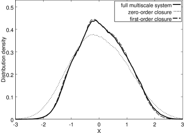
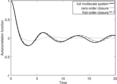
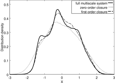
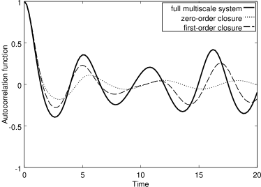
$F_{x}=8,\quad\varepsilon=0.1$
Distribution density function Autocorrelation function

$F_{x}=8,\quad\varepsilon=0.01$
Distribution density function Autocorrelation function

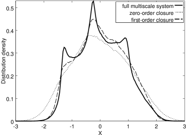
Figure 1: Distribution density and autocorrelation functions of slow variables.

To more systematically compare DDFs for many parameter regimes, we introduce two metrics on the space of distributions. First is the Jensen-Shannon metric which is derived from the information-theoretic Kullback-Leibler divergence [25] and is given by

$$m_{\mathrm{JS}}(P,Q)=\frac{1}{\sqrt{2}}\left(\int_{-\infty}^{\infty}\log\left(\frac{2p(x)}{p(x)+q(x)}\right)p(x)dx+\int_{-\infty}^{\infty}\log\left(\frac{2q(x)}{p(x)+q(x)}\right)q(x)dx\right)^{1/2},$$ (6.31)

where $p$ and $q$ are densities on distributions $P$ and $Q$. The next metric we consider is the earth mover’s distance [41], which measures the minimum energy needed to move one DDF to another as though they were piles of dirt; the energy cost is the amount of ‘dirt’ times the distance it moved. One nice property is that the distance between two delta distributions $\delta_{\alpha}$ and $\delta_{\beta}$ is simply $|\alpha-\beta|$. For distribution functions of one-dimensional random variables, the earth-mover’s distance is the $L^{1}$ norm of the difference of the cumulative distributions:

$$m_{\mathrm{EM}}(P,Q)=\int_{-\infty}^{\infty}\left|\int_{-\infty}^{x}p(s)-q(s)\mathrm{d}s\right|\mathrm{d}x.$$ (6.32)

Figure 2 shows distances between reduced systems DDFs and the corresponding multiscale slow variable DDFs. A variety of regimes is considered, with coupling parameters $\lambda_{x},\lambda_{y}\in[0.1,1]$, forcing parameters $F_{x}\in\{6,7,8,10,16\}$ and $F_{y}\in\{8,12,16\}$, and timescale separations $\varepsilon\in\{10^{-1},10^{-2}\}$. The data points are plotted with respect to coupling parameter $\lambda_{x}$. For each regime considered, the corresponding distances are shown for both zero-order and first-order reduced systems.

Jensen-Shannon metric	Earth mover’s distance

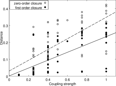
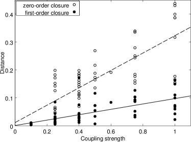
Figure 2: Distances between DDFs of reduced and multiscale systems

As the coupling strength between fast and slow systems increases, it is apparently more difficult for the reduced systems to capture the correct slow dynamics of the multiscale system, as suggested by the linear best-fit curves. It should be noted that this correlation is slightly weaker when plotted against $\lambda_{y}$, the coupling parameter for the fast system. However, the distribution densities of the first-order reduced system are consistently closer in both metrics than the zero-order system to the multiscale system.

6.2 Mean state response to small perturbations

In this section we examine the response of the mean state $\langle\boldsymbol{x}\rangle$ of the slow variables (that is, $h(\boldsymbol{x})=\boldsymbol{x}$ in (3.5)) in the Lorenz ’96 system to two simple types of small external forcing:

1. Heaviside step forcing

   $$\delta\boldsymbol{f}_{\mathrm{H}}(t)=\begin{cases}0&\text{if }t<0,\\ \boldsymbol{v}_{\mathrm{H}}&\text{if }t>0,\end{cases}$$

2. Ramp forcing

   $$\delta\boldsymbol{f}_{\mathrm{ramp}}(t)=\begin{cases}0&\text{if }t<0,\\ t\boldsymbol{v}_{\mathrm{ramp}}&\text{if }t>0,\end{cases}$$

where $\boldsymbol{v}_{\mathrm{H}}$ and $\boldsymbol{v}_{\mathrm{ramp}}$ are constant vectors. To compute the response of the mean state $\langle\boldsymbol{x}\rangle$, we generate an initial ensemble sampled from a trajectory that has been given sufficient time to settle onto the attractor. For each ensemble member we let evolve a short trajectory under the unperturbed dynamics as well as the under the perturbed dynamics, then we take the difference between these two trajectories and average over the entire ensemble. Here we consider forcing of the form $\boldsymbol{v}=\alpha\hat{e}_{j}$, where $\alpha$ is constant and $\hat{e}_{j}$ a standard basis vector in $\mathbb{R}^{N_{x}}$. In the translation-invariant Lorenz ’96 system, without loss of generality we need only consider a single such vector, say $\hat{e}_{0}$. Figure 3 shows the mean response of the slow variables to small Heaviside forcing in the two-time rescaled Lorenz ’96 system, where the magnitude of the forcing $|\boldsymbol{v}_{\mathrm{H}}|$ is $1\%$ of $|\boldsymbol{f}|$ averaged over the invariant distribution.

Figure 3: Mean response of $\boldsymbol{x}$ to step forcing at node $x_{11}$. $N_{x}=20,\ N_{y}=80,\ F_{x}=16,\ F_{y}=12,\ \lambda_{x}=0.4,\ \lambda_{y}=0.4,\ \varepsilon=0.1$

Since the external forcing is sufficiently small to consider the response of the mean state approximately linear, we use the ideal response operator of Gritsun and Dymnikov [20] (also see [1, 2, 3, 9, 8, 10, 11, 27]) by generating mean responses for several perturbations and computing the linear best least-squares fit. This is a time-dependent matrix, and due to the symmetry of the Lorenz ’96 system the dimensionality is reduced by one so that we have simply a time-dependent vector. With the ideal response operator, the response to a multitude of forcings can be readily estimated. We verify the nonlinearity in the actual response in Figure 4, which shows the growth in time of the relative error between the ideal response and the actual response to small Heaviside step forcing, averaged over several different forcings. We limit the plot to 5 time units because the large features of the Heaviside response are mostly fully developed by that time. Note in particular that the response is more linear in the reduced system, which is probably due to the fact that the Lyapunov exponents in the reduced system are much smaller than those in the two-scale system.

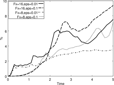
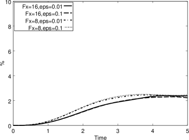
Mean relative error of ideal response Multiscale system Reduced system

Figure 4: Nonlinearity of response: relative error ideal response vs actual nonlinear response.

We now compare the ideal responses of the full and reduced systems. The snapshots of the ideal responses for the two-scale and reduced models (as well as the linear response approximation, described in the next section) at times $T=2$ and $T=5$ are shown in Figures 5 and 6 for the Heaviside and ramp forcing, respectively. The response is captured accurately at the node which is directly forced (here $x_{11}$), but capturing the off-diagonal response as the perturbation propagates through the system is more difficult. Indeed, it seems that in the zero-order reduced systems the propagation speed is slightly faster than in the two-scale systems, but for the first-order reduced systems the response is well captured.

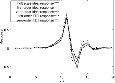
Response to Heaviside forcing. $F_{x}=16,\ \varepsilon=0.1$ Response to Heaviside forcing. $F_{x}=8,\ \varepsilon=0.1$
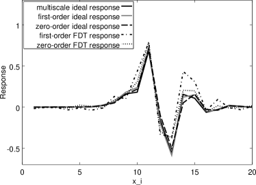
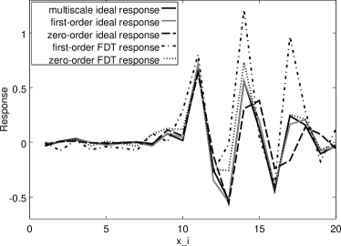
Response to Heaviside forcing. $F_{x}=8,\ \varepsilon=0.01$

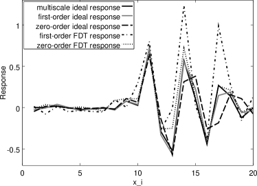
Figure 5: Snapshots of the response operators for the response time $T=2$ (left), and $T=5$ (right), Heaviside forcing.

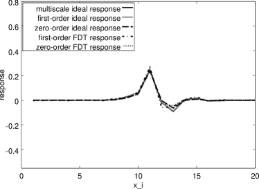
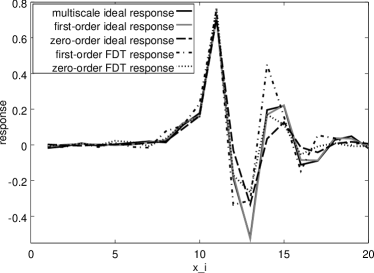
Response to ramp forcing. $F_{x}=16,\ \varepsilon=0.1$ Response to ramp forcing. $F_{x}=8,\ \varepsilon=0.1$ Response to ramp forcing. $F_{x}=8,\ \varepsilon=0.01$

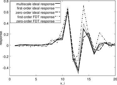
Figure 6: Snapshots of the response operators for the response time $T=2$ (left), and $T=5$ (right), ramp forcing.

It is more clear to see the quantitative differences in Figures 7 and 8 which show the relative distance between the responses as well as their cosine similarity $\frac{\boldsymbol{u}\cdot\boldsymbol{v}}{\|\boldsymbol{u}\|\|\boldsymbol{v}\|}$ versus time for Heaviside step forcing and ramp forcing, respectively. Also shown in these figures are the linear responses computed using the reduced system statistics, as described in the next section.

Response to Heaviside forcing. $F_{x}=16,\ \varepsilon=0.1$ Relative error Cosine similarity

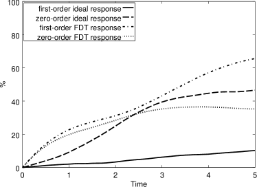
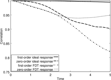
Response to Heaviside forcing. $F_{x}=8,\ \varepsilon=0.1$ Relative error Cosine similarity

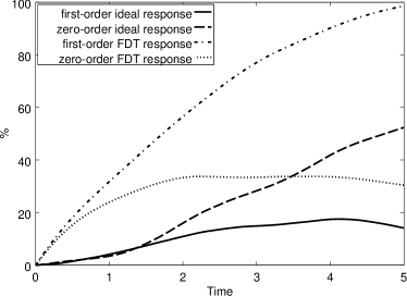
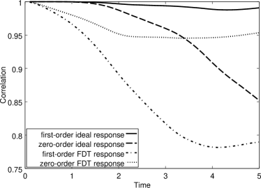
Response to Heaviside forcing. $F_{x}=8,\ \varepsilon=0.01$ Relative error Cosine similarity

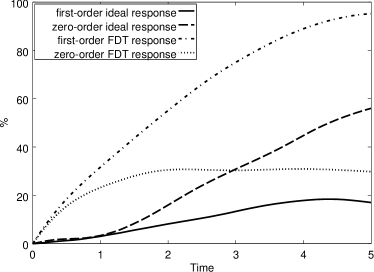
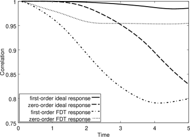
Figure 7: Comparing multiscale ideal response with reduced system ideal & quasi-Gaussian response operators for Heaviside forcing

Response to ramp forcing. $F_{x}=16,\ \varepsilon=0.1$ Relative error Cosine similarity

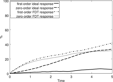
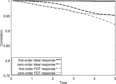
Ramp forcing. $F_{x}=8,\ \varepsilon=0.1$ Relative error Cosine similarity

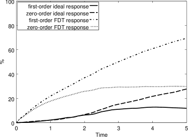
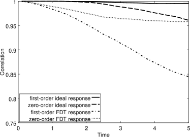
Response to ramp forcing. $F_{x}=8,\ \varepsilon=0.01$ Relative error Cosine similarity

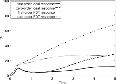
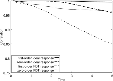
Figure 8: Comparing multiscale ideal response with reduced system ideal & quasi-Gaussian response operators for ramp forcing

We observe that the first-order reduced system ideal response is a much closer approximation to the multiscale ideal response than the corresponding zero-order ideal response. In these regimes the relative error of the first-order response is limited to about $20\%$ for the Heaviside forcing and less for the ramp forcing, while in the zero-order system the error is around $40\%$ for the step forcing and $30\%$ for ramp forcing at time $t=5$. Remark that in the third plot for ramp forcing response in Figure 8 there is a small bump in the relative error shortly after the onset of forcing. This plot corresponds to a weakly chaotic regime ($F_{x}=8,F_{y}=12$) with a large timescale separation ($\varepsilon=10^{-2}$) in the multiscale system. In this regime the small nonlinear fluctuations of the multiscale system are relatively large compared to the ramp forcing for $t$ near zero, so the relative error of the reduced system responses is large.

6.3 Predicting the response of the two-scale system via linear response approximation of the reduced system

Above in Section 6.2 we discussed the actual responses of the statistical mean states of both the two-scale and reduced models to small Heaviside and ramp forcings. For completeness of the study, we also attempt to predict the response of the mean state of the two-scale system via the quasi-Gaussian linear response approximation [1, 2, 3, 9, 9, 8, 10, 11, 27] of the reduced system. In the quasi-Gaussian response approximation, the terms $\bar{b}(\boldsymbol{x})$ and $b_{A}(\boldsymbol{x})$ in (3.19) are replaced with the Gaussian approximations with same mean state and covariance matrices as in the actual dynamics. This, and the fact that $h(\boldsymbol{x})=\boldsymbol{x}$ in (3.5) yields the following formula for the linear response approximation of the mean state response:

$$\begin{array}[]{c}\displaystyle\delta\langle\boldsymbol{x}\rangle(t)=\int_{0}^{t}\boldsymbol{R}(t-s)\delta\boldsymbol{f}(s)\mathrm{d}s,\\ \displaystyle\boldsymbol{R}(t)=\lim_{r\rightarrow\infty}\frac{1}{r}\int_{0}^{r}\boldsymbol{x}(\tau+t))(\boldsymbol{x}(\tau)-\boldsymbol{\bar{x}})^{T}\mathrm{d}\tau\,\Sigma^{-1},\end{array}$$ (6.33a)

$$\begin{array}[]{c}\displaystyle\delta\langle\boldsymbol{x}\rangle_{A}(t)=\int_{0}^{t}\boldsymbol{R}_{A}(t-s)\delta\boldsymbol{f}(s)\mathrm{d}s,\\ \displaystyle\boldsymbol{R}_{A}(t)=\lim_{r\rightarrow\infty}\frac{1}{r}\int_{0}^{r}\boldsymbol{x}_{A}(\tau+t))(\boldsymbol{x}_{A}(\tau)-\boldsymbol{\bar{x}}_{A})^{T}\mathrm{d}\tau\,\Sigma_{A}^{-1},\end{array}$$ (6.33b)

where $\boldsymbol{\bar{x}}$ and $\Sigma$ are the mean state and covariance matrix of the corresponding unperturbed systems (two-scale and reduced), computed as

$$\boldsymbol{\bar{x}}=\lim_{r\rightarrow\infty}\frac{1}{r}\int_{0}^{r}\boldsymbol{x}(\tau)\mathrm{d}\tau,$$ (6.34a)

$$\Sigma=\lim_{r\rightarrow\infty}\frac{1}{r}\int_{0}^{r}(\boldsymbol{x}(\tau)-\boldsymbol{\bar{x}})(\boldsymbol{x}(\tau)-\boldsymbol{\bar{x}})^{T}\mathrm{d}\tau.$$ (6.34b)

For large multiscale problems the mean response may be difficult to compute directly, since the large ensemble size needed for an accurate average is compounded by an already large number of variables and small timestep discretization. In the case where the mean response of the slow variables is desired, one might prefer to compute the FDT response (6.33) using a time series from the reduced system for a “quick and dirty” approximation to the ideal response operator for the multiscale slow system. We show the accuracy of this FDT response approximation for the Lorenz ’96 system, using a quasi-Gaussian approximation with time series data from the zero- and first-order reduced systems. The quasi-Gaussian response snapshots for the response times $T=2$ and $T=5$ are shown in Figures 5 and 6 for the Heaviside and ramp forcing, respectively. Qualitatively, the quasi-Gaussian response does capture the large features of the actual response, although most noticeable in these snapshots is the large exaggeration of the quasi-Gaussian response calculated from the first-order reduced system, which predicts a much larger off-diagonal response than what is observed. The possible reason for that is that the distribution densities of the first-order reduced model are more strongly non-Gaussian than those of the zero-order reduced model, while the time autocorrelation functions are more weakly decaying (see Figure 1). It was observed previously in [27] that in these conditions the quasi-Gaussian linear response approximation tends to overshoot the off-diagonal response by a large margin. In other words, the better precision of the quasi-Gaussian linear response of the zero-order model is the result of mutual cancellation of the two errors: first one is the error in the distribution density of the zero-order reduced model (significantly more Gaussian than in in the multiscale dynamics), while the second one is the error in the quasi-Gaussian linear response due to non-Gaussianity of the statistical state (less in the case of the zero-order model).

The relative error and cosine similarity are measured against the multiscale ideal response and can be seen for Heaviside step forcing in Figure 7 and for ramp forcing in Figure 8. The ideal response of the first-order reduced system is clearly the best of the four responses at capturing response in the slow variables. It is interesting, but perhaps not too surprising, that the least accurate estimate is given by the FDT response of the first-order reduced system. This should be expected since the quasi-Gaussian approximation is only valid for well-mixing systems whose distribution densities are close to Gaussian, which in particular is the case for the uncoupled Lorenz ’96 systems in a chaotic regime $F\geq 8$. However, such a system exhibits suppressed chaos when coupled to another chaotic systems, and the resulting distribution density will be far from Gaussian [5]. Since the first-order reduced system matches more closely the multiscale system, and the zero-order system will behave as an uncoupled Lorenz ’96 system, the first-order system will be less chaotic and will be a poor candidate for the quasi-Gaussian FDT response. In fact, for non-chaotic regimes, as in the case of $F_{x}=7,\ F_{y}=12$ where spatially periodic solutions emerge in the two-scale and first-order reduced systems, the long-time covariance matrix $\Sigma$ will be singular, so the quasi-Gaussian response as presented will not be applicable. For further reading on blended FDT responses which might be more effective in these cases, see [8].

7 Summary

In this work we studied the response to small external perturbations of multiscale dynamics and their reduced models for slow variables only. We elucidated a set of criteria for statistical properties of the multiscale and reduced systems which facilitated similarity of responses of both systems to small external perturbations. It was shown that the similarity of marginal distribution densities of slow variables and their time autocorrelation functions controlled the similarity of responses to small external perturbations of both systems.

Like in [4], here we demonstrated that including a first-order correction term to a standard closure approximation for a nonlinear chaotic two-time system offered distinct improvements over the zero-order closure in capturing large-scale features of the slow dynamics. In particular, this reduced system was able to accurately capture the distribution density of solutions as well as the mean state response of the system to simple forcing perturbations. This correction term was relatively easy to generate, requiring only simple statistical calculations of the uncoupled fast system for an appropriate set of fixed parameters, and the resulting reduced system required much less computational resources than the corresponding multiscale system.

Focusing on the mean state linear response of the slow variables, we showed that forcing perturbations in the reduced systems have similar responses as in the two-time system. Furthermore, we showed that using the unperturbed dynamics of the reduced systems for linear response prediction is also possible. However, in the parameter regimes we present here the first-order reduced systems are not rapidly mixing and do not follow a Gaussian distribution, but the zero-order reduced systems do have these properties, so this fluctuation-dissipation response is effective only using the zero-order system. A linear response method which takes into account the non-Gaussianity of the invariant statistical state (such as the blended response algorithm [9, 8, 10, 11], based on the tangent map linear response approximation) is apparently needed to capture the response for strongly non-Gaussian dynamical regimes in reduced models.

Here the linear response closure derivation and numerical results have been presented only for the special case of linear coupling between slow and fast systems, but this derivation has been extended to systems with nonlinear and multiplicative coupling [6]. In future work we hope to extend similar results to these more general systems and to test the robustness of this method for application to a large variety of problems.

Acknowledgment. Rafail Abramov was supported by the National Science Foundation CAREER grant DMS-0845760, and the Office of Naval Research grants N00014-09-0083 and 25-74200-F6607. Marc Kjerland was supported as a Research Assistant through the National Science Foundation CAREER grant DMS-0845760.

References

- [1] R.V. Abramov. Short-time linear response with reduced-rank tangent map. Chin. Ann. Math., 30B(5):447–462, 2009.
- [2] R.V. Abramov. Approximate linear response for slow variables of deterministic or stochastic dynamics with time scale separation. J. Comput. Phys., 229(20):7739–7746, 2010.
- [3] R.V. Abramov. Improved linear response for stochastically driven systems. Front. Math. China, 7(2):199–216, 2012.
- [4] R.V. Abramov. A simple linear response closure approximation for slow dynamics of a multiscale system with linear coupling. Multiscale Model. Simul., 10(1):28–47, 2012.
- [5] R.V. Abramov. Suppression of chaos at slow variables by rapidly mixing fast dynamics through linear energy-preserving coupling. Commun. Math. Sci., 10(2):595–624, 2012.
- [6] R.V. Abramov. A simple closure approximation for slow dynamics of a multiscale system: Nonlinear and multiplicative coupling. Multiscale Model. Simul., 11(1):134–151, 2013.
- [7] R.V. Abramov. A simple stochastic parameterization for reduced models of multiscale dynamics. Multiscale Model. Simul., 2013. submitted.
- [8] R.V. Abramov and A.J. Majda. Blended response algorithms for linear fluctuation-dissipation for complex nonlinear dynamical systems. Nonlinearity, 20:2793–2821, 2007.
- [9] R.V. Abramov and A.J. Majda. New approximations and tests of linear fluctuation-response for chaotic nonlinear forced-dissipative dynamical systems. J. Nonlin. Sci., 18(3):303–341, 2008.
- [10] R.V. Abramov and A.J. Majda. New algorithms for low frequency climate response. J. Atmos. Sci., 66:286–309, 2009.
- [11] R.V. Abramov and A.J. Majda. Low frequency climate response of quasigeostrophic wind-driven ocean circulation. J. Phys. Oceanogr., 42:243–260, 2012.
- [12] R. Azencott, A. Beri, and I. Timofeyev. Sub-sampling and parametric estimation for multiscale dynamics. Comm. Math. Sci., 2012. to appear.
- [13] G. Branstator. Low-frequency patterns induced by stationary waves. J. Atmos. Sci., 47:629–648, 1990.
- [14] G. Branstator and J. Berner. Linear and nonlinear signatures in planetary wave dynamics of an AGCM: phase space tendencies. J. Atmos. Sci., 62:1792–1811, 2005.
- [15] R. Buizza, M. Miller, and T. Palmer. Stochastic representation of model uncertainty in the ECMWF Ensemble Prediction System. Q. J. R. Meteor. Soc., 125:2887–2908, 1999.
- [16] D.T. Crommelin and E. Vanden-Eijnden. Subgrid scale parameterization with conditional Markov chains. J. Atmos. Sci., 65:2661–2675, 2008.
- [17] I. Fatkullin and E. Vanden-Eijnden. A computational strategy for multiscale systems with applications to Lorenz 96 model. J. Comp. Phys., 200:605–638, 2004.
- [18] C. Franzke and A.J. Majda. Low-order stochastic mode reduction for a prototype atmospheric GCM. J. Atmos. Sci., 63:457–479, 2006.
- [19] C. Franzke, A.J. Majda, and E. Vanden-Eijnden. Low-order stochastic model reduction for a realistic barotropic model climate. J. Atmos. Sci., 62:1722–1745, 2005.
- [20] A. Gritsun and V. Dymnikov. Barotropic atmosphere response to small external actions. theory and numerical experiments. Atmos. Ocean Phys., 35(5):511–525, 1999.
- [21] K. Hasselmann. Stochastic climate models, part I, theory. Tellus, 28:473–485, 1976.
- [22] M.A. Katsoulakis and G.D. Vlachos. Hierarchical kinetic monte carlo simulations for diffusion of interacting molecules. J. Chem. Phys., 112:9412–9427, 2003.
- [23] B. Khouider, A.J. Majda, and M.A. Katsoulakis. Coarse grained stochastic models for tropical convection. Proc. Natl. Acad. Sci., 100:11941–11946, 2003.
- [24] S. Kravtsov, D. Kondrashov, and M. Ghil. Multilevel regression modeling of nonlinear processes: Derivation and applications to climatic variability. J. Clim., 18(21):4404–4424, 2005.
- [25] S. Kullback and R. Leibler. On information and sufficiency. Ann. Math. Stat., 22:79–86, 1951.
- [26] E. Lorenz. Predictability: A problem partly solved. In Proceedings of the Seminar on Predictability, Shinfield Park, Reading, England, 1996. ECMWF.
- [27] A.J. Majda, R.V Abramov, and M.J. Grote. Information Theory and Stochastics for Multiscale Nonlinear Systems, volume 25 of CRM Monograph Series of Centre de Recherches Mathématiques, Université de Montréal. American Mathematical Society, 2005. ISBN 0-8218-3843-1.
- [28] A.J. Majda, C. Franzke, and D.T. Crommelin. Normal forms for reduced stochastic climate models. Proc. Natl. Acad. Sci., 97:12413–12417, 2009.
- [29] A.J. Majda, B. Gershgorin, and Y. Yuan. Low frequency response and fluctuation-dissipation theorems: Theory and practice. J. Atmos. Sci., 67:1186–1201, 2010.
- [30] A.J. Majda and B. Khouider. Stochastic and mesoscopic models for tropical convection. Proc. Natl. Acad. Sci., 99:1123–1128, 2002.
- [31] A.J. Majda, I. Timofeyev, and E. Vanden-Eijnden. Models for stochastic climate prediction. Proc. Natl. Acad. Sci., 96:14687–14691, 1999.
- [32] A.J. Majda, I. Timofeyev, and E. Vanden-Eijnden. A mathematical framework for stochastic climate models. Comm. Pure Appl. Math., 54:891–974, 2001.
- [33] A.J. Majda, I. Timofeyev, and E. Vanden-Eijnden. A priori tests of a stochastic mode reduction strategy. Physica D, 170:206–252, 2002.
- [34] A.J. Majda, I. Timofeyev, and E. Vanden-Eijnden. Systematic strategies for stochastic mode reduction in climate. J. Atmos. Sci., 60:1705–1722, 2003.
- [35] A.J. Majda and X. Wang. Linear response theory for statistical ensembles in complex systems with time-periodic forcing. Comm. Math. Sci., 8(1):145–172, 2010.
- [36] M. Newman, P.D. Sardeshmukh, and C. Penland. Stochastic forcing of the wintertime extratropical flow. J. Atmos. Sci., 54:435–455, 1997.
- [37] T. Palmer. A nonlinear dynamical perspective on model error: A proposal for nonlocal stochastic-dynamic parameterization in weather and climate prediction models. Q. J. R. Meteor. Soc., 127:279–304, 2001.
- [38] G. Papanicolaou. Introduction to the asymptotic analysis of stochastic equations. In R. DiPrima, editor, Modern modeling of continuum phenomena, volume 16 of Lectures in Applied Mathematics. American Mathematical Society, 1977.
- [39] G. Pavliotis and A. Stuart. Multiscale Methods: Averaging and Homogenization. Springer, 2008.
- [40] H. Risken. The Fokker-Planck Equation. Springer-Verlag, New York, 2nd edition, 1989.
- [41] Y. Rubner, C. Tomasi, and L.J. Guibas. The earth mover’s distance as a metric for image retrieval. Int. J. Comput. Vision, 40(2):99–121, 2000.
- [42] D. Ruelle. Chaotic Evolution and Strange Attractors. Cambridge University Press, 1989.
- [43] D. Ruelle. Differentiation of SRB states. Comm. Math. Phys., 187:227–241, 1997.
- [44] D. Ruelle. General linear response formula in statistical mechanics, and the fluctuation-dissipation theorem far from equilibrium. Phys. Lett. A, 245:220–224, 1998.
- [45] G. Uhlenbeck and L. Ornstein. On the theory of the Brownian motion. Phys. Rev., 36:823–841, 1930.
- [46] E. Vanden-Eijnden. Numerical techniques for multiscale dynamical systems with stochastic effects. Comm. Math. Sci., 1:385–391, 2003.
- [47] V.M. Volosov. Averaging in systems of ordinary differential equations. Russian Math. Surveys, 17:1–126, 1962.
- [48] J.S. Whitaker and P.D. Sardeshmukh. A linear theory of extratropical synoptic eddy statistics. J. Atmos. Sci., 55:237–258, 1998.
- [49] D. Wilks. Effects of stochastic parameterizations in the Lorenz ’96 system. Q. J. R. Meteorol. Soc., 131:389–407, 2005.
- [50] L.-S. Young. What are SRB measures, and which dynamical systems have them? J. Stat. Phys., 108(5-6):733–754, 2002.
- [51] Y. Zhang and I.M. Held. A linear stochastic model of a GCM’s midlatitude storm tracks. J. Atmos. Sci., 56:3416–3435, 1999.