A simple and efficient numerical method for computing the dynamics of rotating Bose-Einstein condensates via a rotating Lagrangian coordinate

Abstract

We propose a simple, efficient and accurate numerical method for simulating the dynamics of rotating Bose-Einstein condensates (BECs) in a rotational frame with/without a long-range dipole-dipole interaction. We begin with the three-dimensional (3D) Gross-Pitaevskii equation (GPE) with an angular momentum rotation term and/or long-range dipole-dipole interaction, state the two-dimensional (2D) GPE obtained from the 3D GPE via dimension reduction under anisotropic external potential and review some dynamical laws related to the 2D and 3D GPE. By introducing a rotating Lagrangian coordinate system, the original GPEs are re-formulated to GPEs without the angular momentum rotation which is replaced by a time-dependent potential in the new coordinate system. We then cast the conserved quantities and dynamical laws in the new rotating Lagrangian coordinates. Based on the new formulation of the GPE for rotating BECs in the rotating Lagrangian coordinates, a time-splitting spectral method is presented for computing the dynamics of rotating BECs. The new numerical method is explicit, simple to implement, unconditionally stable and very efficient in computation. It is spectral order accurate in space and second-order accurate in time, and conserves the mass in the discrete level. Extensive numerical results are reported to demonstrate the efficiency and accuracy of the new numerical method. Finally, the numerical method is applied to test the dynamical laws of rotating BECs such as the dynamics of condensate width, angular momentum expectation and center-of-mass, and to investigate numerically the dynamics and interaction of quantized vortex lattices in rotating BECs without/with the long-range dipole-dipole interaction.

1 Introduction

Bose–Einstein condensation (BEC), first observed in 1995 [4, 17, 22], has provided a platform to study the macroscopic quantum world. Later, with the observation of quantized vortices [36, 33, 34, 38, 2, 48, 18], rotating BECs have been extensively studied in the laboratory. The occurrence of quantized vortices is a hallmark of the superfluid nature of Bose–Einstein condensates. In addition, condensation of bosonic atoms and molecules with significant dipole moments whose interaction is both nonlocal and anisotropic has recently been achieved experimentally in trapped ⁵²Cr and ¹⁶⁴Dy gases [26, 32, 31, 1, 21, 35, 46].

At temperatures $T$ much smaller than the critical temperature $T_{c}$, the properties of a BEC in a rotating frame with long-range dipole-dipole interaction are well described by the macroscopic complex-valued wave function $\psi=\psi({\bf x},t)$, whose evolution is governed by the three-dimensional (3D) Gross-Pitaevskii equation (GPE) in dimensionless units with angular momentum rotation term and long-range dipole-dipole interaction [52, 47, 45, 9, 19, 1, 40]:

(1.1) $$i\partial_{t}\psi({{\bf x}},t)=\left[-\frac{1}{2}\nabla^{2}+V({\bf x})+\kappa|\psi|^{2}+\lambda\left(U_{\rm dip}*|\psi|^{2}\right)-\Omega L_{z}\right]\psi({\bf x},t),$$

where $t$ denotes time, ${\bf x}=(x,y,z)^{T}\in{\mathbb{R}}^{3}$ is the Cartesian coordinate vector, $V({\bf x})$ is a given real-valued external trapping potential which is determined by the type of system under investigation and $\kappa=\frac{4\pi Na_{s}}{x_{s}}$ is a dimensionless constant describing the strength of the short-range two-body interaction (positive for repulsive interaction, and resp. negative for attractive interaction) of a condensate consisting of $N$ particles with $s$-wave scattering length $a_{s}$ and a dimensionless length unit $x_{s}$ [9, 19]. Furthermore $\Omega\in{\mathbb{R}}$ is a given dimensionless constant representing the angular velocity, and $\lambda=\frac{mN\mu_{0}\mu_{\rm dip}^{2}}{3\hbar^{2}x_{s}}$ is a dimensionless constant describing the strength of the long-range dipole-dipole interaction with $m$ the mass of a particle, $\mu_{0}$ the vacuum permeability, $\mu_{\rm dip}$ the permanent magnetic dipole moment (e.g. $\mu_{\rm dip}=6\mu_{{}_{B}}$ for ⁵²C_r with $\mu_{{}_{B}}$ being the Bohr magneton) and $\hbar$ the Planck constant [9, 19, 40]. In addition, $L_{z}$ is the dimensionless $z$-component of the angular momentum rotation defined as

(1.2) $$L_{z}=-i(x\partial_{y}-y\partial_{x}),$$

and $U_{\rm dip}$ is the dimensionless long-range dipole-dipole interaction potential defined as

(1.3) $$U_{\rm dip}({\bf x})=\frac{3}{4\pi|{\bf x}|^{3}}\left[1-\frac{3({\bf x}\cdot{\bf n})^{2}}{|{\bf x}|^{2}}\right]=\frac{3}{4\pi|{\bf x}|^{3}}\left[1-3\cos^{2}(\vartheta)\right],\qquad{\bf x}\in{\mathbb{R}}^{3},$$

with ${\bf n}=(n_{1},n_{2},n_{3})^{T}\in{\mathbb{R}}^{3}$ a given unit vector, i.e. $|{\bf n}|=\sqrt{n_{1}^{2}+n_{2}^{2}+n_{3}^{2}}=1$, representing the dipole axis (or dipole moment) and $\vartheta=\vartheta_{\bf n}({\bf x})$ the angle between the dipole axis ${\bf n}$ and the vector ${\bf x}$ [9, 19]. The wave function is normalized to

(1.4) $$\|\psi\|^{2}:=\int_{{\mathbb{R}}^{3}}|\psi({\bf x},t)|^{2}\,d{\bf x}=1.$$

In addition, similar to [9, 19], the above GPE (1.1) can be re-formulated as the following Gross-Pitaevskii-Poisson system [9, 6, 19]

(1.5) $$i\partial_{t}\psi({{\bf x}},t)=\left[-\frac{1}{2}\nabla^{2}+V({\bf x})+(\kappa-\lambda)|\psi|^{2}-3\lambda\varphi({\bf x},t)-\Omega L_{z}\right]\psi({\bf x},t),$$

(1.6) $$\varphi({\bf x},t)=\partial_{{\bf n}{\bf n}}u({\bf x},t),\quad-\nabla^{2}u({\bf x},t)=|\psi({\bf x},t)|^{2}\ \ \hbox{with}\ \ \lim_{|{\bf x}|\to\infty}u({\bf x},t)=0,$$

where $\partial_{\bf n}={\bf n}\cdot\nabla$ and $\partial_{{\bf n}{\bf n}}=\partial_{\bf n}(\partial_{\bf n})$. From (1.6), it is easy to see that

(1.7) $$u({\bf x},t)=\left(\frac{1}{4\pi|{\bf x}|}\right)*|\psi|^{2}:=\int_{{\mathbb{R}}^{3}}\frac{1}{4\pi|{\bf x}-{\bf x}^{\prime}|}|\psi({\bf x}^{\prime},t)|^{2}d{\bf x}^{\prime},\quad{\bf x}\in{\mathbb{R}}^{3},\quad t\geq 0.$$

In some physical experiments of rotating BEC, the external trap is strongly confined in the $z$-direction, i.e.

(1.8) $$V({\bf x})=V_{2}(x,y)+\frac{z^{2}}{2\varepsilon^{4}},\qquad{\bf x}\in{\mathbb{R}}^{3},$$

with $0<\varepsilon\ll 1$ a given dimensionless parameter [6], resulting in a pancake-shaped BEC. Similar to the case of a non-rotating BEC, formally the GPE (1.1) or (1.5)-(1.6) can effectively be approximated by a two-dimensional (2D) GPE as [10, 9, 19]:

(1.9) $$\qquad i\partial_{t}\psi({{\bf x}_{\perp}},t)=\left[-\frac{1}{2}\nabla_{\perp}^{2}+V_{2}({\bf x}_{\perp})+\frac{\kappa+\lambda(3n_{3}^{2}-1)}{\varepsilon\sqrt{2\pi}}|\psi|^{2}-\frac{3\lambda}{2}\varphi-\Omega L_{z}\right]\psi,$$

(1.10) $$\qquad\varphi=\varphi({\bf x}_{\perp},t)=\left(\partial_{{\bf n}_{\perp}{\bf n}_{\perp}}-n_{3}^{2}\nabla_{\perp}^{2}\right)u({\bf x}_{\perp},t),\quad{\bf x}_{\perp}=(x,y)^{T}\in{\mathbb{R}}^{2},\ t\geq 0,$$

where $\nabla_{\perp}=(\partial_{x},\partial_{y})^{T}$, $\nabla_{\perp}^{2}=\partial_{xx}+\partial_{yy}$, ${\bf n}_{\perp}=(n_{1},n_{2})^{T}$, $\partial_{{\bf n}_{\perp}}={\bf n}_{\perp}\cdot\nabla_{\perp}$, $\partial_{{\bf n}_{\perp}{\bf n}_{\perp}}=\partial_{{\bf n}_{\perp}}(\partial_{{\bf n}_{\perp}})$ and

(1.11) $$u({\bf x}_{\perp},t)=G^{\varepsilon}*|\psi|^{2},\quad G^{\varepsilon}({\bf x}_{\perp})=\frac{1}{(2\pi)^{3/2}}\int_{\mathbb{R}}\frac{e^{-s^{2}/2}}{\sqrt{|{\bf x}_{\perp}|^{2}+\varepsilon^{2}s^{2}}}ds,\quad{\bf x}_{\perp}\in{\mathbb{R}}^{2}.$$

The above problem (1.9)-(1.10) with (1.11) is usually called surface adiabatic model (SAM) for a rotating BEC with dipole-dipole interaction in 2D. Furthermore, taking $\varepsilon\to 0^{+}$ in (1.11), we obtain

(1.12) $$G^{\varepsilon}({\bf x}_{\perp})\to\frac{1}{2\pi|{\bf x}_{\perp}|}:=G^{0}({\bf x}_{\perp}),\qquad{\bf x}_{\perp}\in{\mathbb{R}}^{2}.$$

This, together with (1.11), implies that when $\varepsilon\to 0^{+}$,

(1.13) $$u({\bf x}_{\perp},t)=\frac{1}{2\pi|{\bf x}_{\perp}|}*|\psi|^{2}\Longleftrightarrow(-\nabla_{\perp}^{2})^{1/2}u=|\psi|^{2}\quad\hbox{with}\ \lim_{|{\bf x}_{\perp}|\to\infty}u({\bf x}_{\perp},t)=0.$$

The problem (1.9)-(1.10) with (1.13) is usually called surface density model (SDM) for a rotating BEC with dipole-dipole interaction in 2D. Note that even for the SDM we retain the $\varepsilon$-dependence in (1.9).

In fact, the GPE (1.1) or (1.5) in 3D and the SAM or SDM in 2D can be written in a unified way in $d$-dimensions ($d=2$ or $3$) with ${\bf x}=(x,y)^{T}$ when $d=2$ and ${\bf x}=(x,y,z)^{T}$ when $d=3$:

(1.14) $$i\partial_{t}\psi({{\bf x}},t)=\left[-\frac{1}{2}\nabla^{2}+V({\bf x})+\beta|\psi|^{2}+\eta\varphi({\bf x},t)-\Omega L_{z}\right]\psi({{\bf x}},t),$$

(1.15) $$\varphi({\bf x},t)=L_{\bf n}u({\bf x},t),\qquad u({\bf x},t)=G*|\psi|^{2},\qquad{\bf x}\in{\mathbb{R}}^{d},\quad t\geq 0,$$

where $V({\bf x})=V_{2}({\bf x})$ when $d=2$ and

(1.16) $$\beta=\left\{\begin{array}[]{l}\frac{\kappa+\lambda(3n_{3}^{2}-1)}{\varepsilon\sqrt{2\pi}},\\ \kappa-\lambda,\\ \end{array}\right.\quad\eta=\left\{\begin{array}[]{l}-3\lambda/2,\\ -3\lambda,\\ \end{array}\right.\quad L_{\bf n}=\left\{\begin{array}[]{ll}\partial_{\bf n_{\bot}n_{\bot}}-n_{3}^{2}\nabla^{2},&d=2,\\ \partial_{\bf nn},&d=3,\end{array}\right.$$

(1.17) $$G({\bf x})=\left\{\begin{array}[]{l}1/2\pi|{\bf x}|,\\ G^{\varepsilon}({\bf x}),\\ 1/4\pi|{\bf x}|,\\ \end{array}\right.\Longleftrightarrow\widehat{G}(\xi)=\left\{\begin{array}[]{ll}1/|\xi|,&d=2\ \&\ \hbox{SDM},\\ \frac{1}{2\pi^{2}}\int_{\mathbb{R}}\frac{e^{-\varepsilon^{2}s^{2}/2}}{|\xi|^{2}+s^{2}}ds,&d=2\ \&\ \hbox{SAM},\\ 1/|\xi|^{2},&d=3,\\ \end{array}\right.$$

where $\widehat{f}(\xi)$ denotes the Fourier transform of the function $f({\bf x})$ for ${\bf x},\,\xi\in{\mathbb{R}}^{d}$. For studying the dynamics of a rotating BEC, the following initial condition is used:

(1.18) $$\psi({\bf x},0)=\psi_{0}({\bf x}),\qquad{\bf x}\in{\mathbb{R}}^{d},\qquad\mbox{with}\quad\|\psi_{0}\|^{2}:=\int_{\mathbb{R}^{d}}|\psi_{0}({\bf x})|^{2}\,d{\bf x}=1.$$

We remark here that in most BEC experiments, the following dimensionless harmonic potential is used

(1.19) $$V({\bf x})=\frac{1}{2}\left\{\begin{array}[]{ll}\gamma_{x}^{2}x^{2}+\gamma_{y}^{2}y^{2},&d=2,\\ \gamma_{x}^{2}x^{2}+\gamma_{y}^{2}y^{2}+\gamma_{z}^{2}z^{2},&d=3,\end{array}\right.$$

where $\gamma_{x}>0$, $\gamma_{y}>0$ and $\gamma_{z}>0$ are dimensionless constants proportional to the trapping frequencies in $x$-, $y$- and $z$-direction, respectively.

Recently, many numerical and theoretical studies have been done on rotating (dipolar) BECs. There have been many numerical methods proposed to study the dynamics of non-rotating BECs, i.e. when $\Omega=0$ and $\eta=0$ [20, 3, 28, 11, 14, 43, 37]. Among them, the time-splitting sine/Fourier pseudospectral method is one of the most successful methods. Compared to other methods, the time-splitting pseudospectral method has spectral accuracy in space and is easy to implement. In addition, as was shown in [9], this method can also be easily generalized to simulate the dynamics of dipolar BECs when $\eta\neq 0$. However, in rotating condensates, i.e. when $\Omega\neq 0$, we can not directly apply the time-splitting pseudospectral method proposed in [14] to study their dynamics due to the appearance of angular rotational term. So far, there have been several methods introduced to solve the GPE with an angular momentum term. For example, a pseudospectral type method was proposed in [10] by reformulating the problem in the two-dimensional polar coordinates $(r,\theta)$ or three-dimensional cylindrical coordinates $(r,\theta,z)$. The method is of second-order or fourth-order in the radial direction and spectral accuracy in other directions. A time-splitting alternating direction implicit method was proposed in [13], where the authors decouple the angular terms into two parts and apply the Fourier transform in each direction. Furthermore, a generalized Laguerre-Fourier-Hermite pseudospectral method was presented in [12]. These methods have higher spatial accuracy compared to those in [3, 28, 8] and are also valid in dissipative variants of the GPE (1.1), cf. [44]. On the other hand, the implementation of these methods can become quite involved. The aim of this paper is to propose a simple and efficient numerical method to solve the GPE with angular momentum rotation term which may include a dipolar interaction term. One novel idea in this method consists in the use of rotating Lagrangian coordinates as in [5] in which the angular momentum rotation term vanishes. Hence, we can easily apply the methods for non-rotating BECs in [14] to solve the rotating case.

This paper is organized as follows. In Section 2, we present the dynamical laws of rotating dipolar BECs based on the GPE (1.14)–(1.18). Then in Section 3, we introduce a coordinate transformation and cast the GPE and its dynamical quantities in the new coordinate system. Numerical methods are proposed in Section 4 to discretize the GPE for both the two-dimensional and three-dimensional cases. In Section 5, we report on the accuracy of our methods and present some numerical results. We make some concluding remarks in Section 6.

2 Dynamical properties

In this section, we analytically study the dynamics of rotating dipolar BECs. We present dynamical laws, including the conservation of angular momentum expectation, the dynamics of condensate widths and the dynamics of the center of mass. In the following we omit the proofs for brevity; they are similar to the ones in [14, 10].

2.1 Conservation of mass and energy

The GPE in (1.14)–(1.18) has two important invariants: the mass (or normalization) of the wave function, which is defined as

(2.1) $$N(t):=\|\psi(\cdot,t)\|^{2}:=\int_{{\mathbb{R}}^{d}}|\psi({{\bf x}},t)|^{2}d{\bf x}\equiv\int_{{\mathbb{R}}^{d}}|\psi({\bf x},0)|^{2}d{\bf x}=1,\qquad t\geq 0,$$

and the energy per particle

(2.2) $$E(t) := E(\psi(\cdot,t))=\int_{{\mathbb{R}}^{d}}\left[\frac{1}{2}|\nabla\psi|^{2}+V({\bf x})|\psi|^{2}+\frac{\beta}{2}|\psi|^{4}+\frac{\eta}{2}\varphi|\psi|^{2}-\Omega\psi^{*}L_{z}\psi\right]d{\bf x}$$

$$\equiv E(\psi(\cdot,0))=E(\psi_{0}),\qquad t\geq 0,$$

where $f^{*}$ denotes the conjugate of the complex-valued function $f$. Stationary states, corresponding to critical points of the energy defined in (2.2), play an important role in the study of rotating dipolar BECs. Usually, to find stationary states $\phi_{s}({\bf x})$, one can use the ansatz

(2.3) $$\psi({\bf x},t)=e^{-i\mu_{s}t}\phi_{s}({\bf x}),\qquad{\bf x}\in{\mathbb{R}}^{d},\quad t\geq 0,$$

where $\mu_{s}\in{\mathbb{R}}$ is the chemical potential. Substituting (2.3) into (1.14) yields the nonlinear eigenvalue problem

(2.4) $$\mu_{s}\phi_{s}({{\bf x}})=\left[-\frac{1}{2}\nabla^{2}+V({\bf x})+\beta|\phi_{s}|^{2}+\eta\varphi_{s}-\Omega L_{z}\right]\phi_{s}({\bf x}),\quad\ {\bf x}\in{\mathbb{R}}^{d},$$

(2.5) $$\varphi_{s}({\bf x})=L_{\bf n}u_{s}({\bf x}),\qquad u_{s}({\bf x})=G*|\phi_{s}|^{2},\qquad{\bf x}\in{\mathbb{R}}^{d},$$

under the constraint

(2.6) $$\|\phi_{s}\|^{2}=\int_{\mathbb{R}^{d}}|\phi_{s}({\bf x})|^{2}d{\bf x}=1.$$

Thus, by solving the constrained nonlinear eigenvalue problem (2.4)–(2.6), one can find the stationary states of rotating dipolar BECs. In physics literature, the stationary state with the lowest energy is called ground state, while those with larger energy are called excited states.

2.2 Conservation of angular momentum expectation

The angular momentum expectation of a condensate is defined as [14, 10]

(2.7) $$\langle L_{z}\rangle(t)=\int_{{\mathbb{R}}^{d}}\psi^{*}({\bf x},t)L_{z}\psi({\bf x},t)\,d{\bf x},\qquad t\geq 0.$$

This quantity is often used to measure the vortex flux. The following lemma describes the dynamics of angular momentum expectation in rotating dipolar BECs.

Lemma 1.

Suppose that $\psi({\bf x},t)$ solves the GPE (1.14)–(1.18) with $V({\bf x})$ chosen as the harmonic potential (1.19). Then we have

(2.8) $$\qquad\frac{d\langle L_{z}\rangle(t)}{dt}=(\gamma_{x}^{2}-\gamma_{y}^{2})\int_{{\mathbb{R}}^{d}}xy|\psi|^{2}d{\bf x}-\eta{\int_{{\mathbb{R}}^{d}}|\psi|^{2}\left[(x\partial_{y}-y\partial_{x})\varphi\right]d{\bf x}},\quad t\geq 0.$$

Furthermore, if the following two conditions are satisfied: (i) $\gamma_{x}=\gamma_{y}$ and (ii) $\eta=0$ for any given initial data $\psi_{0}$ in (1.18) or ${\bf n}=(0,0,1)^{T}$ when $\psi_{0}$ satisfies $\psi_{0}({\bf x})=f(r)e^{im\theta}$ in 2D and $\psi_{0}({\bf x})=f(r,z)e^{im\theta}$ in 3D with ${m\in\mathbb{Z}}$ and $f$ a function of $r$ in 2D or $(r,z)$ in 3D, then the angular momentum expectation is conserved, i.e.

(2.9) $$\langle L_{z}\rangle(t)\equiv\langle L_{z}\rangle(0),\quad t\geq 0.$$

That is, in a radially symmetric trap in 2D or a cylindrically symmetric trap in 3D, the angular momentum expectation is conserved when either there is no dipolar interaction for any initial data or the dipole axis is parallel to the $z$-axis with a radially/cylindrically symmetric or central vortex-type initial data.

2.3 Dynamics of condensate width

The condensate width of a BEC in $\alpha$-direction (where $\alpha=x,y,z$ or $r=\sqrt{x^{2}+y^{2}}$) is defined by

(2.10) $$\sigma_{\alpha}(t)=\sqrt{\delta_{\alpha}(t)},\quad\ t\geq 0,\qquad\mbox{where}\quad\delta_{\alpha}(t)=\int_{{\mathbb{R}}^{d}}\alpha^{2}|\psi({\bf x},t)|^{2}d{\bf x}.$$

In particular, when $d=2$, we have the following lemma for its dynamics [10]:

Lemma 2.

Consider two-dimensional BECs with radially symmetric harmonic trap (1.19), i.e. $d=2$ and $\gamma_{x}=\gamma_{y}:=\gamma_{r}$. If $\eta=0$, then for any initial datum $\psi_{0}({\bf x})$ in (1.18), it holds for $t\geq 0$

(2.11) $$\qquad\delta_{r}(t)=\frac{E(\psi_{0})+\Omega\langle L_{z}\rangle(0)}{\gamma_{r}^{2}}[1-\cos(2\gamma_{r}t)]+\delta_{r}^{(0)}\cos(2\gamma_{r}t)+\frac{\delta_{r}^{(1)}}{2\gamma_{r}}\sin(2\gamma_{r}t),$$

where $\delta_{r}(t):=\delta_{x}(t)+\delta_{y}(t)$, $\delta_{r}^{(0)}:=\delta_{x}(0)+\delta_{y}(0)$ and $\delta_{r}^{(1)}:=\dot{\delta}_{x}(0)+\dot{\delta}_{y}(0)$. Furthermore, if the initial condition $\psi_{0}({\bf x})$ is radially symmetric, we have

(2.12) $$\delta_{x}(t) = \delta_{y}(t)\;=\;\frac{1}{2}\delta_{r}(t)$$

$$= \frac{E(\psi_{0})+\Omega\langle L_{z}\rangle(0)}{2\gamma_{x}^{2}}[1-\cos(2\gamma_{x}t)]+\delta_{x}^{(0)}\cos(2\gamma_{x}t)+\frac{\delta_{x}^{(1)}}{2\gamma_{x}}\sin(2\gamma_{x}t),\ t\geq 0.$$

Thus, in this case the condensate widths $\sigma_{x}(t)$ and $\sigma_{y}(t)$ are periodic functions with frequency doubling trapping frequency.

2.4 Dynamics of center of mass

We define the center of mass of a condensate at any time $t$ by

(2.13) $${\bf x}_{c}(t)=\int_{\mathbb{R}^{d}}{\bf x}\,|\psi({\bf x},t)|^{2}d{\bf x},\qquad t\geq 0.$$

The following lemma describes the dynamics of the center of mass.

Lemma 3.

Suppose that $\psi({\bf x},t)$ solves the GPE (1.14)–(1.18) with $V({\bf x})$ chosen as the harmonic potential (1.19). Then for any given initial data $\psi_{0}$, the dynamics of the center of mass are governed by the following second-order ODEs:

(2.16) $$\ddot{{\bf x}}_{c}(t)-2\Omega{J}\dot{{\bf x}}_{c}(t)+({\Lambda}+\Omega^{2}{J^{2}})\,{\bf x}_{c}(t)=0,\qquad t\geq 0,\qquad\qquad\qquad$$

$${\bf x}_{c}(0)={\bf x}_{c}^{(0)}:=\int_{\mathbb{R}^{d}}{\bf x}|\psi_{0}|^{2}d{\bf x},\qquad$$

$$\dot{{\bf x}}_{c}(0)={\bf x}_{c}^{(1)}:=\int_{\mathbb{R}^{d}}{\rm Im}\left(\psi_{0}^{*}\nabla\psi_{0}\right)d{\bf x}-\Omega{J}{\bf x}_{c}^{(0)},$$

where ${\rm Im}(f)$ denotes the imaginary part of the function $f$ and the matrices

$${J}=\left(\begin{array}[]{cc}0&1\\ -1&0\end{array}\right),\qquad{\Lambda}=\left(\begin{array}[]{cc}\gamma_{x}^{2}&0\\ 0&\gamma^{2}_{y}\end{array}\right),\qquad\mbox{for\quad$d=2$},$$

or

$${J}=\left(\begin{array}[]{ccc}0&1&0\\ -1&0&0\\ 0&0&0\end{array}\right),\qquad{\Lambda}=\left(\begin{array}[]{ccc}\gamma_{x}^{2}&0&0\\ 0&\gamma^{2}_{y}&0\\ 0&0&\gamma_{z}^{2}\end{array}\right),\qquad\mbox{for\quad$d=3$}.$$

Lemma 3 shows that the dynamics of the center of mass depends on the trapping frequencies and the angular velocity, but it is independent of the interaction strength constants $\beta$ and $\eta$ in (1.14). For analytical solutions to the second-order ODEs (2.16)-(2.16), we refer to [51].

2.5 An analytical solution under special initial data

From Lemma 3, we can construct an analytical solution to the GPE (1.14)–(1.18) when the initial data is chosen as a stationary state with its center shifted.

Lemma 4.

Suppose $V({\bf x})$ in (1.14) is chosen as the harmonic potential (1.19) and the initial condition $\psi_{0}({\bf x})$ in (1.18) is chosen as

(2.19) $$\psi_{0}({\bf x})=\phi_{s}({\bf x}-{\bf x}^{0}),\qquad{\bf x}\in{\mathbb{R}}^{d},$$

where ${\bf x}^{0}\in{\mathbb{R}}^{d}$ is a given point and $\phi_{s}({\bf x})$ is a stationary state defined in (2.4)–(2.6) with chemical potential $\mu_{s}$, then the exact solution of (1.14)–(1.18) can be constructed as

(2.20) $$\psi({\bf x},t)=\phi_{s}({\bf x}-{\bf x}_{c}(t))\,e^{-i\mu_{s}t}\,e^{iw({\bf x},t)},\qquad{\bf x}\in{\mathbb{R}}^{d},\quad t\geq 0,$$

where ${\bf x}_{c}(t)$ satisfies the ODE (2.16) with

(2.21) $${\bf x}_{c}(0)={\bf x}^{0},\qquad\dot{{\bf x}}_{c}(0)=-\Omega{J}{\bf x}^{0},$$

and $w({\bf x},t)$ is linear in ${\bf x}$, i.e.

$$w({\bf x},t)={\bf c}(t)\cdot{\bf x}+g(t),\quad{\bf c}(t)=(c_{1}(t),\ldots,c_{d}(t))^{T},\quad{\bf x}\in{\mathbb{R}}^{d},\ \ t\geq 0$$

for some functions ${\bf c}(t)$ and $g(t)$. Thus, up to phase shifts, $\psi$ remains a stationary state with shifted center at all times.

3 GPE under a rotating Lagrangian coordinate

In this section, we first introduce a coordinate transformation and derive the GPE in transformed coordinates. Then we reformulate the dynamical quantities studied in Section 2 in the new coordinate system.

3.1 A rotating Lagrangian coordinate transformation

For any time $t\geq 0$, let ${A}(t)$ be an orthogonal rotational matrix defined as

(3.3) $${A}(t)=\left(\begin{array}[]{cc}\cos(\Omega t)&\sin(\Omega t)\\ -\sin(\Omega t)&\cos(\Omega t)\end{array}\right),\quad\ \ \mbox{if \ \ $d=2$,}\qquad\quad\ \$$

and

(3.7) $${A}(t)=\left(\begin{array}[]{ccc}\cos(\Omega t)&\sin(\Omega t)&0\\ -\sin(\Omega t)&\cos(\Omega t)&0\\ 0&0&1\end{array}\right),\quad\ \ \mbox{if \ \ $d=3$.}\qquad$$

It is easy to verify that $A^{-1}(t)=A^{T}(t)$ for any $t\geq 0$ and ${A}(0)={I}$ with $I$ the identity matrix. For any $t\geq 0$, we introduce the rotating Lagrangian coordinates $\widetilde{\bf x}$ as [5, 23, 27]

(3.8) $$\widetilde{\bf x}={A}^{-1}(t){\bf x}=A^{T}(t){\bf x}\quad\Leftrightarrow\quad{\bf x}={A}(t){\widetilde{\bf x}},\qquad{\bf x}\in{\mathbb{R}}^{d},$$

and denote the wave function in the new coordinates as $\phi:=\phi(\widetilde{\bf x},t)$

(3.9) $$\phi(\widetilde{\bf x},t):=\psi({\bf x},t)=\psi\left({A}(t){\widetilde{\bf x}},t\right),\qquad{\bf x}\in{\mathbb{R}}^{d},\quad t\geq 0.$$

In fact, here we refer the Cartesian coordinates ${\bf x}$ as the Eulerian coordinates and Fig. 1 depicts the geometrical relation between the Eulerian coordinates ${\bf x}$ and the rotating Lagrangian coordinates $\widetilde{\bf x}$ for any fixed $t\geq 0$.

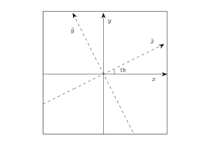
Fig. 1: Cartesian (or Eulerian) coordinates $(x,y)$ (solid) and rotating Lagrangian coordinates $(\tilde{x},\tilde{y})$ (dashed) in 2D for any fixed $t\geq 0$.

Using the chain rule, we obtain the derivatives

$$\qquad\partial_{t}\phi(\widetilde{\bf x},t)=\partial_{t}\psi({\bf x},t)+\nabla\psi({\bf x},t)\cdot\left(\dot{A}(t)\widetilde{\bf x}\right)=\partial_{t}\psi({\bf x},t)-\Omega(x\partial_{y}-y\partial_{x})\psi({\bf x},t),$$

$$\qquad\nabla\phi(\widetilde{\bf x},t)={A^{-1}}(t)\nabla\psi({\bf x},t),\qquad\nabla^{2}\phi(\widetilde{\bf x},t)=\nabla^{2}\psi({\bf x},t).$$

Substituting them into (1.14)–(1.18) gives the following $d$-dimensional GPE in the rotating Lagrangian coordinates:

(3.10) $$\qquad i\partial_{t}\phi(\widetilde{{\bf x}},t)=\left[-\frac{1}{2}\nabla^{2}+W(\widetilde{{\bf x}},t)+\beta|\phi|^{2}+\eta\varphi(\widetilde{\bf x},t)\right]\phi(\widetilde{\bf x},t),\quad\widetilde{\bf x}\in{\mathbb{R}}^{d},\quad t>0,$$

(3.11) $$\qquad\varphi(\widetilde{\bf x},t)=L_{{\bf m}(t)}u(\widetilde{\bf x},t),\qquad u(\widetilde{\bf x},t)=G*|\phi|^{2},\qquad\widetilde{\bf x}\in{\mathbb{R}}^{d},\quad t\geq 0,$$

where $G$ is defined in (1.17) and

(3.12) $$W(\widetilde{\bf x},t)=V(A(t)\widetilde{\bf x}),\qquad\widetilde{\bf x}\in{\mathbb{R}}^{d},$$

(3.15) $$L_{{\bf m}(t)}=\left\{\begin{array}[]{ll}\partial_{{\bf m}_{\perp}(t){\bf m}_{\perp}(t)}-n_{3}^{2}\nabla^{2},&d=2,\\ \partial_{{\bf m}(t){\bf m}(t)},&d=3,\end{array}\right.\quad t\geq 0,$$

with ${\bf m}(t)\in{\mathbb{R}}^{3}$ and ${\bf m}_{\perp}(t)\in{\mathbb{R}}^{2}$ defined as

(3.16) $${\bf m}(t)=\left(\begin{array}[]{c}m_{1}(t)\\ m_{2}(t)\\ m_{3}(t)\end{array}\right):={A}^{-1}(t){\bf n}=\left(\begin{array}[]{c}n_{1}\cos(\Omega t)-n_{2}\sin(\Omega t)\\ n_{1}\sin(\Omega t)+n_{2}\cos(\Omega t)\\ n_{3}\end{array}\right),\quad t\geq 0,$$

and ${\bf m}_{\perp}(t)=(m_{1}(t),m_{2}(t))^{T}$, respectively. The initial data transforms as

(3.17) $$\phi(\widetilde{\bf x},0)=\psi({\bf x},0)=\psi_{0}({\bf x}):=\phi_{0}({\bf x})=\phi_{0}(\widetilde{\bf x}),\qquad\widetilde{\bf x}={\bf x}\in{\mathbb{R}}^{d}.$$

We remark here again that if $V({\bf x})$ in (1.14) is a harmonic potential as defined in (1.19), then the potential $W(\widetilde{\bf x},t)$ in (3.10) has the form

$$W(\widetilde{\bf x},t)=\frac{1}{4}\left\{\begin{array}[]{ll}{\omega}_{1}({\widetilde{x}}^{2}+{\widetilde{y}}^{2})+{\omega}_{2}\left[({\widetilde{x}}^{2}-{\widetilde{y}}^{2})\cos(2\Omega t)+2{\widetilde{x}}{\widetilde{y}}\sin(2\Omega t)\right],&d=2,\\ \omega_{1}({\widetilde{x}}^{2}+{\widetilde{y}}^{2})+\omega_{2}\left[({\widetilde{x}}^{2}-{\widetilde{y}}^{2})\cos(2\Omega t)+2{\widetilde{x}}{\widetilde{y}}\sin(2\Omega t)\right]+2\gamma_{z}^{2}{\widetilde{z}}^{2},&d=3,\\ \end{array}\right.$$

where $\omega_{1}=\gamma_{x}^{2}+\gamma_{y}^{2}$ and $\omega_{2}=\gamma_{x}^{2}-\gamma_{y}^{2}$. It is easy to see that when $\gamma_{x}=\gamma_{y}:=\gamma_{r}$, i.e. radially and cylindrically symmetric harmonic trap in 2D and 3D, respectively, we have $\omega_{1}=2\gamma_{r}^{2}$ and $\omega_{2}=0$ and thus the potential $W(\widetilde{\bf x},t)=V(\widetilde{\bf x})$ becomes time-independent.

In contrast to (1.14), the GPE (3.10) does not have an angular momentum rotation term, which enables us to develop simple and efficient numerical methods for simulating the dynamics of rotating dipolar BEC in Section 4.

3.2 Dynamical quantities

In the above, we introduced rotating Lagrangian coordinates and cast the GPE in the new coordinate system. Next we consider the dynamical laws in terms of the new wave function $\phi({\widetilde{\bf x}},t)$.

Mass and energy. In rotating Lagrangian coordinates, the conservation of mass (2.1) yields

(3.19) $$\qquad\|\psi(\cdot,t)\|^{2}:=\int_{{\mathbb{R}}^{d}}|\psi({\bf x},t)|^{2}d{\bf x}=\int_{\mathbb{R}^{d}}|\phi(\widetilde{\bf x},t)|^{2}d\widetilde{\bf x}=\|\phi(\cdot,t)\|^{2}\equiv 1,\quad\ t\geq 0.$$

The energy defined in (2.2) becomes

$$\widetilde{E}(\phi(\cdot,t))=\int_{{\mathbb{R}}^{d}}\left[\frac{1}{2}|\nabla\phi|^{2}+W(\widetilde{\bf x},t)|\phi|^{2}+\frac{\beta}{2}|\phi|^{4}+\frac{\eta}{2}\varphi|\phi|^{2}\right]d\widetilde{\bf x}$$

(3.20) $$\qquad\qquad-\int_{{\mathbb{R}}^{d}}\int_{0}^{t}\Big{[}\partial_{\tau}W(\widetilde{\bf x},\tau)+\frac{\eta}{2}(\partial_{\tau}L_{{\bf m}(\tau)})u(\widetilde{\bf x},\tau)\Big{]}|\phi|^{2}d\tau\,d\widetilde{\bf x}\equiv\widetilde{E}(\phi(\cdot,0)),\quad t\geq 0,$$

where $u$ is given in (3.11). Specifically, it holds

$$\partial_{t}L_{{\bf m}(t)}=2\begin{cases}\partial_{\dot{A}^{T}(t){\bf n}_{\perp}}\partial_{A^{T}(t){\bf n}_{\perp}},\qquad&d=2,\\ \partial_{\dot{A}^{T}(t){\bf n}}\partial_{A^{T}(t){\bf n}},\quad&d=3.\\ \end{cases}$$

Angular momentum expectation. The angular momentum expectation in the new coordinates becomes

(3.21) $$\langle L_{z}\rangle(t) = -i\int_{\mathbb{R}^{d}}\psi^{*}({\bf x},t)(x\partial_{y}-y\partial_{x})\psi({\bf x},t)\,d{\bf x}$$

$$= -i\int_{\mathbb{R}^{d}}\phi^{*}(\widetilde{\bf x},t)({\widetilde{x}}\partial_{\tilde{y}}-{\widetilde{y}}\partial_{\tilde{x}})\phi(\widetilde{\bf x},t)\,d\widetilde{\bf x},\quad\ t\geq 0,$$

which has the same form as (2.7) in the new coordinates of $\widetilde{\bf x}\in{\mathbb{R}^{d}}$ and the wave function $\phi(\widetilde{\bf x},t)$. Indeed, if we denote $\widetilde{L}_{z}$ as the $z$-component of the angular momentum in the rotating Lagrangian coordinates, we have $\widetilde{L}_{z}=-i({\widetilde{x}}\partial_{\tilde{y}}-{\widetilde{y}}\partial_{\tilde{x}})=-i(x\partial_{y}-y\partial_{x})=L_{z}$, i.e. the coordinate transform does not change the angular momentum in $z$-direction. In addition, noticing that for any $t\geq 0$ it holds $\phi(\widetilde{\bf x},t)=\psi({\bf x},t)$ and $|{A}(t)|=1$ for any $t\geq 0$ immediately yields (3.21).

Condensate width. After the coordinate transform, it holds

(3.22) $$\delta_{r}(t)=\int_{\mathbb{R}^{d}}(x^{2}+y^{2})|\psi|^{2}d{\bf x}=\int_{\mathbb{R}^{d}}({\widetilde{x}}^{2}+{\widetilde{y}}^{2})|\phi|^{2}d\widetilde{\bf x}=\delta_{\tilde{x}}(t)+\delta_{\tilde{y}}(t),$$

(3.23) $$\delta_{z}(t)=\int_{\mathbb{R}^{d}}z^{2}|\psi|^{2}d{\bf x}=\int_{\mathbb{R}^{d}}{\widetilde{z}}^{2}|\phi|^{2}d\widetilde{\bf x}=\delta_{\tilde{z}}(t),$$

for any $t\geq 0$.

Center of mass. The center of mass in rotating Lagrangian coordinates is defined as

(3.24) $$\widetilde{\bf x}_{c}(t)=\int_{\mathbb{R}^{d}}\widetilde{\bf x}\,|\phi(\widetilde{\bf x},t)|^{2}d\widetilde{\bf x},\qquad t\geq 0.$$

Since $\det(A(t))=1$ for any $t\geq 0$, it holds that ${\bf x}_{c}(t)=A(t)\widetilde{\bf x}_{c}(t)$ for any time $t\geq 0$. In rotating Lagrangian coordinates, we have the following analogue of Lemma 4:

Lemma 5.

Suppose $V({\bf x})$ in (1.14) is chosen as the harmonic potential (1.19) and the initial condition $\phi_{0}(\widetilde{\bf x})$ in (3.17) is chosen as

(3.25) $$\phi_{0}(\widetilde{\bf x})={\phi_{s}}(\widetilde{\bf x}-\widetilde{\bf x}^{0}),\qquad\widetilde{\bf x}\in{\mathbb{R}}^{d},$$

where $\widetilde{\bf x}^{0}$ is a given point in ${\mathbb{R}}^{d}$ and ${\phi_{s}}(\widetilde{\bf x})$ is a stationary state defined in (2.4)–(2.6) with chemical potential ${\mu_{s}}$, then the exact solution of (3.10)–(3.11) is of the form

(3.26) $$\phi(\widetilde{\bf x},t) = {\phi_{s}}(\widetilde{\bf x}-\widetilde{\bf x}_{c}(t))\,e^{-i{\mu_{s}}t}\,e^{i\widetilde{w}(\widetilde{\bf x},t)},\qquad t>0,$$

where $\widetilde{\bf x}_{c}(t)$ satisfies the second-order ODEs:

(3.27) $$\ddot{\widetilde{\bf x}}_{c}(t)+A^{T}(t)\Lambda A(t)\,\widetilde{\bf x}_{c}(t)={\bf 0},\qquad t\geq 0,\qquad\qquad\qquad$$

(3.28) $$\widetilde{\bf x}_{c}(0)=\widetilde{\bf x}^{0},\quad\dot{\widetilde{\bf x}}_{c}(0)={\bf 0},$$

with the matrix $\Lambda$ defined in Lemma 3 and $\widetilde{w}(\widetilde{\bf x},t)$ is linear in $\widetilde{\bf x}$, i.e.

$$\widetilde{w}(\widetilde{\bf x},t)={\bf\widetilde{c}}(t)\cdot\widetilde{\bf x}+\widetilde{g}(t),\quad{\bf\widetilde{c}}(t)=(\widetilde{c}_{1}(t),\ldots,\widetilde{c}_{d}(t))^{T},\quad{\bf x}\in{\mathbb{R}}^{d},\ \ t\geq 0.$$

We have seen that the form of the transformation matrix ${A}(t)$ in (3.7) is such that the coordinate transformation does not affect the quantities in $z$-direction, e.g. $\langle L_{z}\rangle$, $\sigma_{z}(t)$ and $z_{c}(t)$.

4 Numerical methods

To study the dynamics of rotating dipolar BECs, in this section we propose a simple and efficient numerical method for discretizing the GPE (3.10)–(3.17) in rotating Lagrangian coordinates. The detailed discretizations for both the 2D and 3D GPEs are presented. Here we assume $\Omega\neq 0$, and for $\Omega=0$, we refer to [9, 7, 46, 19].

In practical computations, we first truncate the whole space problem (3.10)–(3.17) to a bounded computational domain $\mathcal{D}\subset{\mathbb{R}}^{d}$ and consider

(4.1) $$\qquad i\partial_{t}\phi(\widetilde{\bf x},t)=-\frac{1}{2}\nabla^{2}\phi+W(\widetilde{\bf x},t)\phi+\beta|\phi|^{2}\phi+\eta\varphi\phi,\quad\widetilde{\bf x}\in{\mathcal{D}},\ t>0,$$

(4.2) $$\qquad\varphi(\widetilde{\bf x},t)=L_{{\bf m}(t)}u(\widetilde{\bf x},t),\quad u(\widetilde{\bf x},t)=\int_{{\mathbb{R}}^{d}}G(\widetilde{\bf x}-\widetilde{\bf y})\rho(\widetilde{\bf y},t)\,d\widetilde{\bf y},\quad\widetilde{\bf x}\in{\mathcal{D}},\ t>0;$$

where

$$\rho(\widetilde{\bf y},t)=\left\{\begin{array}[]{ll}|\phi(\widetilde{\bf y},t)|^{2},&\widetilde{\bf y}\in\mathcal{D},\\ 0,&\hbox{otherwise},\end{array}\right.\qquad\widetilde{\bf y}\in{\mathbb{R}}^{d}.$$

The initial condition is given by

(4.3) $$\phi(\widetilde{\bf x},0)=\phi_{0}(\widetilde{\bf x}),\quad\ \widetilde{\bf x}\in\overline{\mathcal{D}}.$$

The boundary condition to (4.1) will be chosen based on the kernel function $G$ defined in (1.17). Due to the convolution in (4.2), it is natural to consider using the Fourier transform to compute $u(\widetilde{\bf x},t)$. However, from (1.17) and (3.19), we know that $\lim_{\xi\to 0}\widehat{G}(\xi)=\infty$ and $\widehat{|\phi|^{2}}(\xi=0)\neq 0$. As noted for simulating dipolar BECs in 3D [39, 15, 9], there is a numerical locking phenomena, i.e. numerical errors will be bounded below no matter how small the mesh size is, when one uses the Fourier transform to evaluate $u(\widetilde{\bf x},t)$ and/or $\varphi(\widetilde{\bf x},t)$ numerically in (4.2). As noticed in [9, 6], the second (integral) equation in (4.2) can be reformulated into the Poisson equation (1.6) and square-root-Poisson equation (1.13) for 3D and 2D SDM model, respectively. With these PDE formulations for $u(\widetilde{\bf x},t)$, we can truncate them on the domain $\mathcal{D}$ and solve them numerically via spectral method with sine basis functions instead of Fourier basis functions and thus we can avoid using the $0$-modes [9]. Thus in 3D and 2D SDM model, we choose the homogeneous Dirichlet boundary conditions to (4.1). Of course, for the 2D SAM model, one has to use the Fourier transform to compute $u(\widetilde{\bf x},t)$, thus we take the periodic boundary conditions to (4.1).

The computational domain ${\mathcal{D}}\subset{\mathbb{R}}^{d}$ is chosen as ${\mathcal{D}}=[a,b]\times[c,d]$ if $d=2$ and ${\mathcal{D}}=[a,b]\times[c,d]\times[e,f]$ if $d=3$. Due to the confinement of the external potential, the wave function decays exponentially fast as $|\widetilde{\bf x}|\to\infty$. Thus if we choose ${\mathcal{D}}$ to be sufficiently large, the error from the domain truncation can be neglected. As long as we solve $\phi(\widetilde{\bf x},t)$ in the bounded computational domain ${\mathcal{D}}$, we obtain a corresponding solution $\psi({\bf x},t)$ in the domain $A(t){\mathcal{D}}$. As shown in Fig. 2 for the example of a 2D domain, although the domains $A(t){\mathcal{D}}$ for $t\geq 0$, are in general different for different time $t$, they share a common disk which is bounded by the inner green solid circle in Fig. 2. Thus, the value of $\psi({\bf x},t)$ inside the vertical maximal square (the magenta area) which lies fully within the inner disk can be calculated easily by interpolation.

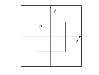
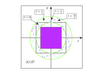
Fig. 2: The bounded computational domain $\mathcal{D}$ in rotating Lagrangian coordinates $\widetilde{\bf x}$ (left) and the corresponding domain $A(t)\mathcal{D}$ in Cartesian (or Eulerian) coordinates ${\bf x}$ (right) when $\Omega=0.5$ at different times: $t=0$ (black solid), $t=\frac{\pi}{4}$ (cyan dashed), $t=\frac{\pi}{2}$ (red dotted) and $t=\frac{3\pi}{4}$ (blue dash-dotted). The two green solid circles determine two disks which are the union (inner circle) and the intersection of all domains $A(t)\mathcal{D}$ for $t\geq 0$, respectively. The magenta area is the vertical maximal square inside the inner circle.

4.1 Time-splitting method

Next, let us introduce a time-splitting method to discretize (4.1)–(4.3). We choose a time-step size $\Delta t>0$ and define the time sequence as $t_{n}=n\Delta t$ for $n\in\mathbb{N}$. Then from $t=t_{n}$ to $t=t_{n+1}$, we numerically solve the GPE (4.1) in two steps. First we solve

(4.4) $$i\partial_{t}\phi(\widetilde{\bf x},t) = -\frac{1}{2}\nabla^{2}\phi(\widetilde{\bf x},t),\quad\ \widetilde{\bf x}\in{\mathcal{D}},\quad t_{n}\leq t\leq t_{n+1}$$

for a time step of length $\Delta t$, and then we solve

(4.5) $$i\partial_{t}\phi(\widetilde{\bf x},t)=\left[W(\widetilde{\bf x},t)+\beta|\phi|^{2}+\eta\varphi\right]\phi(\widetilde{\bf x},t),\quad\ \widetilde{\bf x}\in{\mathcal{D}},\quad t_{n}\leq t\leq t_{n+1},$$

(4.6) $$\varphi(\widetilde{\bf x},t)=L_{{\bf m}(t)}u(\widetilde{\bf x},t),\qquad u(\widetilde{\bf x},t)=\int_{{\mathbb{R}}^{d}}G(\widetilde{\bf x}-\widetilde{\bf y})\rho(\widetilde{\bf y},t)\,d\widetilde{\bf y},$$

for the same time step.

Equation (4.4) can be discretized in space by sine or Fourier pseudospectral methods and then integrated exactly in time. If homogeneous Dirichlet boundary conditions are used, then we choose the sine pseudospectral method to discretize it; otherwise, the Fourier pseudospectral method is used if the boundary conditions are periodic. For more details, see e.g. [14, 9].

On the other hand, we notice that on each time interval $[t_{n},t_{n+1}]$, the problem (4.5)–(4.6) leaves $|\phi(\widetilde{\bf x},t)|$ and hence $u(\widetilde{\bf x},t)$ invariant, i.e. $|\phi(\widetilde{\bf x},t)|=|\phi(\widetilde{\bf x},t_{n})|$ and $u(\widetilde{\bf x},t)=u(\widetilde{\bf x},t_{n})$ for all times $t_{n}\leq t\leq t_{n+1}$. Thus, for $t\in[t_{n},t_{n+1}]$, Eq. (4.5) reduces to

(4.7) $$\qquad i\partial_{t}\phi(\widetilde{\bf x},t)=\left[W(\widetilde{\bf x},t)+\beta|\phi(\widetilde{\bf x},t_{n})|^{2}+\eta\left(L_{{\bf m}(t)}u(\widetilde{\bf x},t_{n})\right)\right]\phi(\widetilde{\bf x},t),\quad\widetilde{\bf x}\in{\mathcal{D}}.$$

Integrating (4.7) in time gives the solution

(4.8) $$\qquad\phi(\widetilde{\bf x},t)=\phi(\widetilde{\bf x},t_{n})\exp\left[-i\left(\beta|\phi(\widetilde{\bf x},t_{n})|^{2}(t-t_{n})+\eta\Phi(\widetilde{\bf x},t)+\int_{t_{n}}^{t}W(\widetilde{\bf x},\tau)d\tau\right)\right]$$

for $\widetilde{\bf x}\in{\mathcal{D}}$ and $t\in[t_{n},t_{n+1}]$, where the function $\Phi(\widetilde{\bf x},t)$ is defined by

(4.9) $$\Phi(\widetilde{\bf x},t)=\int_{t_{n}}^{t}\left[L_{{\bf m}(\tau)}u(\widetilde{\bf x},t_{n})\right]d\tau=\left(\int_{t_{n}}^{t}L_{\bf m(\tau)}\;d\tau\right)u(\widetilde{\bf x},t_{n}).$$

Plugging (3.16) and (3.15) into (4.9), we get

(4.10) $$\Phi(\widetilde{\bf x},t)=\tilde{L}_{d}(t)u(\widetilde{\bf x},t_{n}),\qquad\widetilde{\bf x}\in{\mathcal{D}},\quad t_{n}\leq t\leq t_{n+1},$$

where

$$\tilde{L}_{d}(t)=\left\{\begin{array}[]{ll}[l_{e}^{11}(t)-l_{e}^{33}(t)]\partial_{\tilde{x}\tilde{x}}+[l_{e}^{22}(t)-l_{e}^{33}(t)]\partial_{\tilde{y}\tilde{y}}+l_{e}^{12}(t)\partial_{\tilde{x}\tilde{y}},&d=2,\\ l_{e}^{11}(t)\partial_{\tilde{x}\tilde{x}}+l_{e}^{22}(t)\partial_{\tilde{y}\tilde{y}}+l_{e}^{33}(t)\partial_{\tilde{z}\tilde{z}}+l_{e}^{12}(t)\partial_{\tilde{x}\tilde{y}}+l_{e}^{13}(t)\partial_{\tilde{x}\tilde{z}}+l_{e}^{23}(t)\partial_{\tilde{y}\tilde{z}},&d=3,\end{array}\right.$$

with

$$l_{e}^{11}(t) = \int_{t_{n}}^{t}m_{1}^{2}(\tau)d\tau=\int_{t_{n}}^{t}\left[n_{1}^{2}\cos^{2}(\Omega\tau)+n_{2}^{2}\sin^{2}(\Omega\tau)-n_{1}n_{2}\sin(2\Omega\tau)\right]d\tau$$

$$= \frac{n_{1}^{2}+n_{2}^{2}}{2}(t-t_{n})+\frac{n_{1}^{2}-n_{2}^{2}}{4\Omega}\left[\sin(2\Omega t)-\sin(2\Omega t_{n})\right]+\frac{n_{1}n_{2}}{2\Omega}\left[\cos(2\Omega t)-\cos(2\Omega t_{n})\right],$$

$$l_{e}^{22}(t) = \int_{t_{n}}^{t}m_{2}^{2}(\tau)d\tau=\int_{t_{n}}^{t}\left[n_{2}^{2}\cos^{2}(\Omega\tau)+n_{1}^{2}\sin^{2}(\Omega\tau)+n_{1}n_{2}\sin(2\Omega\tau)\right]d\tau$$

$$= \frac{n_{1}^{2}+n_{2}^{2}}{2}(t-t_{n})-\frac{n_{1}^{2}-n_{2}^{2}}{4\Omega}\left[\sin(2\Omega t)-\sin(2\Omega t_{n})\right]-\frac{n_{1}n_{2}}{2\Omega}\left[\cos(2\Omega t)-\cos(2\Omega t_{n})\right],$$

$$l_{e}^{12}(t) = 2\int_{t_{n}}^{t}m_{1}(\tau)m_{2}(\tau)d\tau=\int_{t_{n}}^{t}\left[(n_{1}^{2}-n_{2}^{2})\sin(2\Omega\tau)+2n_{1}n_{2}\cos(2\Omega t)\right]d\tau$$

$$= \frac{n_{1}^{2}-n_{2}^{2}}{2\Omega}\left[\cos(2\Omega t_{n})-\cos(2\Omega t)\right]+\frac{n_{1}n_{2}}{\Omega}\left[\sin(2\Omega t)-\sin(2\Omega t_{n})\right],$$

$$l_{e}^{13}(t) = 2n_{3}\int_{t_{n}}^{t}m_{1}(\tau)d\tau=2n_{3}\int_{t_{n}}^{t}\left[n_{1}\cos(\Omega\tau)-n_{2}\sin(\Omega\tau)\right]d\tau$$

$$= \frac{2n_{3}}{\Omega}\left[n_{1}\left[\sin(\Omega t)-\sin(\Omega t_{n})\right]+n_{2}\left[\cos(\Omega t)-\cos(\Omega t_{n})\right]\right],$$

$$l_{e}^{23}(t) = 2n_{3}\int_{t_{n}}^{t}m_{2}(\tau)d\tau=2n_{3}\int_{t_{n}}^{t}\left[n_{1}\sin(\Omega\tau)+n_{2}\cos(\Omega\tau)\right]d\tau$$

$$= \frac{2n_{3}}{\Omega}\left[n_{2}\left[\sin(\Omega t)-\sin(\Omega t_{n})\right]-n_{1}\left[\cos(\Omega t)-\cos(\Omega t_{n})\right]\right],$$

$$l_{e}^{33}(t) = \int_{t_{n}}^{t}n_{3}^{2}\,d\tau=n_{3}^{2}(t-t_{n}),\qquad t_{n}\leq t\leq t_{n+1}.$$

In Section 4.2, we will discuss in detail the approximations to $\Phi(\widetilde{\bf x},t)$ in (4.10). In addition, we remark here again that if $V({\bf x})$ in (1.14) is a harmonic potential as defined in (1.19), then the definite integral in (4.8) can be calculated analytically as

$$\int_{t_{n}}^{t}W(\widetilde{\bf x},\tau)d\tau=\frac{1}{4}{\omega}_{1}({\widetilde{x}}^{2}+{\widetilde{y}}^{2})(t-t_{n})+H(\widetilde{\bf x},t)+\frac{1}{2}\left\{\begin{array}[]{ll}0,&d=2,\\ \gamma_{z}^{2}{\widetilde{z}}^{2}(t-t_{n}),&d=3,\\ \end{array}\right.$$

where

$$H(\widetilde{\bf x},t) = \frac{1}{4}\int_{t_{n}}^{t}{\omega}_{2}\left[({\widetilde{x}}^{2}-{\widetilde{y}}^{2})\cos(2\Omega\tau)+2{\widetilde{x}}{\widetilde{y}}\sin(2\Omega\tau)\right]d\tau$$

$$= \frac{{\omega}_{2}}{8\Omega}\left[\left({\widetilde{x}}^{2}-{\widetilde{y}}^{2}\right)\left[\sin(2\Omega t)-\sin(2\Omega t_{n})\right]-2{\widetilde{x}}{\widetilde{y}}\left[\cos(2\Omega t)-\cos(2\Omega t_{n})\right]\right].$$

Of course, for general external potential $V({\bf x})$ in (1.14), the integral of $W(\widetilde{\bf x},\tau)$ in (4.8) might not be found analytically. In this situation, we can simply adopt a numerical quadrature to approximate it, e.g. the Simpson’s rule can be used as

$$\int_{t_{n}}^{t}W(\widetilde{\bf x},\tau)\,d\tau\approx\frac{t-t_{n}}{6}\left[W(\widetilde{\bf x},t_{n})+4W(\widetilde{\bf x},\frac{t_{n}+t}{2})+W(\widetilde{\bf x},t)\right].$$

We remark here that, in practice, we always use the second-order Strang splitting method [42] to combine the two steps in (4.4) and (4.5)–(4.6). That is, from time $t=t_{n}$ to $t=t_{n+1}$, we (i) evolve (4.4) for half time step $\Delta t/2$ with initial data given at $t=t_{n}$; (ii) evolve (4.5)–(4.6)) for one step $\Delta t$ starting with the new data; and (iii) evolve (4.4) for half time step $\Delta t/2$ again with the newer data. For a more general discussion of the splitting method, we refer the reader to [24, 7, 14].

4.2 Computation of $\Phi(\widetilde{\bf x},t)$

In this section, we present approximations to the function $\Phi(\widetilde{\bf x},t)$ in (4.10). From the discussion in the previous subsection, we need only show how to discretize $u(\widetilde{\bf x},t_{n})$ in (4.2) and its second-order derivatives in (4.10).

4.2.1 Surface adiabatic model in 2D

In this case, the function $u(\widetilde{\bf x},t_{n})$ in (4.9) is given by

(4.11) $$u(\widetilde{\bf x},t_{n})=\int_{{\mathbb{R}}^{2}}G(\widetilde{\bf x}-\widetilde{\bf y})\rho(\widetilde{\bf y},t_{n})\,d\widetilde{\bf y},\quad\ \widetilde{\bf x}\in{\mathcal{D}}.$$

with the kernel function $G$ defined in the second line of (1.17). To approximate it, we consider a 2D box $\mathcal{D}$ with periodic boundary conditions.

Let $M$ and $K$ be two even positive integers. Then we make the (approximate) ansatz

(4.12) $$\qquad u(\widetilde{\bf x},t_{n})=\sum_{p=-M/2}^{M/2-1}\sum_{q=-K/2}^{K/2-1}\widehat{u}^{f}_{pq}(t_{n})\,e^{i\nu_{p}^{1}({\widetilde{x}}-a)}e^{i\nu_{q}^{2}({\widetilde{y}}-c)},\qquad\widetilde{\bf x}=({\widetilde{x}},{\widetilde{y}})\in{\mathcal{D}},$$

where $\widehat{u}^{f}_{pq}(t_{n})$ is the Fourier coefficient of $u(\widetilde{\bf x},t_{n})$ corresponding to the frequencies $(p,q)$ and

$$\nu_{p}^{1}=\frac{2p\pi}{b-a},\qquad\nu_{q}^{2}=\frac{2q\pi}{d-c},\qquad(p,q)\in{\mathcal{S}}_{MK}.$$

The index set ${\mathcal{S}}_{MK}$ is defined as

$${\mathcal{S}}_{MK}=\left\{(p,q)\,|\,-\frac{M}{2}\leq p\leq\frac{M}{2}-1,\ -\frac{K}{2}\leq q\leq\frac{K}{2}-1\right\}.$$

We approximate the convolution in (4.11) by a discrete convolution and take its discrete Fourier transform to obtain

(4.13) $$\widehat{u}^{f}_{pq}(t_{n})=\widehat{G}(\nu_{p}^{1},\nu_{q}^{2})\cdot(\widehat{|\phi^{n}|^{2}})^{f}_{pq},\qquad(p,q)\in{\mathcal{S}}_{MK},$$

where $(\widehat{|\phi^{n}|^{2}})^{f}_{pq}$ is the Fourier coefficient corresponding to the frequencies $(p,q)$ of the function $|\phi(\widetilde{\bf x},t_{n})|^{2}$, and $\widehat{G}(\nu_{p}^{1},\nu_{q}^{2})$ are given by (see details in (1.17))

(4.14) $$\widehat{G}(\nu_{p}^{1},\nu_{q}^{2})=\frac{1}{2\pi^{2}}\int_{-\infty}^{\infty}\frac{e^{-\varepsilon^{2}s^{2}/2}}{(\nu_{p}^{1})^{2}+(\nu_{q}^{2})^{2}+s^{2}}ds,\qquad(p,q)\in{\mathcal{S}}_{MK}.$$

Since the integrand in (4.14) decays exponentially fast, in practice we can first truncate it to an interval $[s_{1},s_{2}]$ with $|s_{1}|,s_{2}>0$ sufficiently large and then evaluate the truncated integral by using quadrature rules, e.g. composite Simpson’s or trapezoidal quadrature rule.

Combining (4.10), (4.12) and (4.13), we obtain an approximation of $\Phi(\widetilde{\bf x},t)$ in the solution (4.8) via the Fourier spectral method as

(4.15) $$\qquad\quad\Phi(\widetilde{\bf x},t)=\sum_{p=-M/2}^{M/2-1}\sum_{q=-K/2}^{K/2-1}\left[L(\nu_{p}^{1},\nu_{q}^{2},t)\widehat{G}(\nu_{p}^{1},\nu_{q}^{2})\cdot(\widehat{|\phi^{n}|^{2}})^{f}_{pq}\right]e^{i\nu_{p}^{1}({\widetilde{x}}-a)}e^{i\nu_{q}^{2}({\widetilde{y}}-c)},$$

for time $t_{n}\leq t\leq t_{n+1}$, where the function $L(\xi_{1},\xi_{2},t)$ is defined as

$$L(\xi_{1},\xi_{2},t)=-\left[\left(l_{e}^{11}(t)-l_{e}^{33}(t)\right)\xi_{1}^{2}+\left(l_{e}^{22}(t)-l_{e}^{33}(t)\right)\xi_{2}^{2}+l_{e}^{12}(t)\xi_{1}\xi_{2}\right].$$

4.2.2 Surface density model in 2D

In this case, the function $u(\widetilde{\bf x},t_{n})$ in (4.9) also satisfies the square-root-Poisson equation in (1.13) which can be truncated on the computational domain ${\mathcal{D}}$ with homogeneous Dirichlet boundary conditions as

(4.16) $$(-\nabla^{2})^{1/2}u(\widetilde{\bf x},t_{n})=|\phi(\widetilde{\bf x},t_{n})|^{2},\quad\ \widetilde{\bf x}\in{\mathcal{D}};\qquad u(\widetilde{\bf x},t_{n})|_{\partial{\mathcal{D}}}=0.$$

The above problem can be discretized by using a sine pseudospectral method in which the 0-modes are avoided. Letting $M,K\in\mathbb{N}$, we denote the index set

$${\mathcal{T}}_{MK}=\left\{(p,q)\,|\,1\leq p\leq M-1,\ 1\leq q\leq K-1\right\},$$

and define the functions

$$U_{p,q}(\widetilde{\bf x})=\sin(\mu_{p}^{1}({\widetilde{x}}-a))\sin(\mu_{q}^{2}({\widetilde{y}}-c)),\qquad(p,q)\in{\mathcal{T}}_{MK},\qquad\widetilde{\bf x}=({\widetilde{x}},{\widetilde{y}})\in{\mathcal{D}},$$

where

(4.17) $$\mu_{p}^{1}=\frac{p\pi}{b-a},\qquad\mu_{q}^{2}=\frac{q\pi}{d-c},\qquad(p,q)\in{\mathcal{T}}_{MK}.$$

Assume that

(4.18) $$u(\widetilde{\bf x},t_{n})=\sum_{p=1}^{M-1}\sum_{q=1}^{K-1}\widehat{u}^{s}_{pq}(t_{n})U_{p,q}(\widetilde{\bf x}),\qquad\widetilde{\bf x}\in{\mathcal{D}},$$

where $\widehat{u}^{s}_{pq}(t_{n})$ is the sine transform of $u(\widetilde{\bf x},t_{n})$ at frequencies $(p,q)$. Substituting (4.18) into (4.16) and taking sine transform on both sides, we obtain

(4.19) $$\widehat{u}^{s}_{pq}(t_{n})=\frac{(\widehat{|\phi^{n}|^{2}})^{s}_{pq}}{\sqrt{(\mu_{p}^{1})^{2}+(\mu_{q}^{2})^{2}}},\qquad(p,q)\in{\mathcal{T}}_{MK},$$

where $(\widehat{|\phi^{n}|^{2}})^{s}_{pq}$ is the sine transform of $|\phi(\widetilde{\bf x},t_{n})|^{2}$ at frequencies $(p,q)$.

Combining (4.18), (4.19) and (4.10), we obtain an approximation of $\Phi(\widetilde{\bf x},t)$ in the solution (4.8) via sine spectral method as

(4.20) $$\qquad\quad\Phi(\widetilde{\bf x},t)=\sum_{p=1}^{M-1}\sum_{q=1}^{K-1}\frac{(\widehat{|\phi^{n}|^{2}})^{s}_{pq}}{\sqrt{(\mu_{p}^{1})^{2}+(\mu_{q}^{2})^{2}}}\left[L(\mu_{p}^{1},\mu_{q}^{2},t)U_{p,q}(\widetilde{\bf x})+l_{e}^{12}(t)V_{p,q}(\widetilde{\bf x})\right],$$

where the functions $L(\xi_{1},\xi_{2},t)$ and $V_{p,q}(\widetilde{\bf x})$ are defined as

$$L(\xi_{1},\xi_{2},t)=-\left[\left(l_{e}^{11}(t)-l_{e}^{33}(t)\right)\xi_{1}^{2}+\left(l_{e}^{22}(t)-l_{e}^{33}(t)\right)\xi_{2}^{2}\right],$$

$$V_{p,q}(\widetilde{\bf x})=\partial_{{\widetilde{x}}{\widetilde{y}}}U_{p,q}(\widetilde{\bf x})=\mu_{p}^{1}\mu_{q}^{2}\cos(\mu_{p}^{1}({\widetilde{x}}-a))\cos(\mu_{q}^{2}({\widetilde{y}}-c)),\qquad(p,q)\in{\mathcal{T}}_{MK}.$$

4.2.3 Approximations in 3D

In 3D case, again the function $u(\widetilde{\bf x},t_{n})$ in (4.9) also satisfies the Poisson equation in (1.6) which can be truncated on the computational domain ${\mathcal{D}}$ with homogeneous Dirichlet boundary conditions as

(4.21) $$-\nabla^{2}u(\widetilde{\bf x},t_{n})=|\phi(\widetilde{\bf x},t_{n})|^{2},\quad\widetilde{\bf x}\in{\mathcal{D}};\qquad\qquad u(\widetilde{\bf x},t_{n})|_{\partial{\mathcal{D}}}=0.$$

The above problem can be discretized by using a sine pseudospectral method in which the 0-modes are avoided. Denote the index set

$${\mathcal{T}}_{MKL}=\left\{(p,q,r)\,|\,1\leq p\leq M-1,\ 1\leq q\leq K-1,\ 1\leq r\leq L-1\right\}$$

where $M,K,L>0$ are integers and define the functions

$$U_{p,q,r}(\widetilde{\bf x})=\sin(\mu_{p}^{1}({\widetilde{x}}-a))\sin(\mu_{q}^{2}({\widetilde{y}}-c))\sin(\mu_{r}^{3}({\widetilde{z}}-e)),\quad(p,q,r)\in{\mathcal{T}}_{MKL},$$

where

$$\mu_{r}^{3}=r\pi/(f-e),\qquad 1\leq r\leq L-1.$$

Again, we take the (approximate) ansatz

(4.22) $$\ \ u(\widetilde{\bf x},t_{n})=\sum_{p=1}^{M-1}\sum_{q=1}^{K-1}\sum_{r=1}^{L-1}\widehat{u}^{s}_{pqr}(t_{n})\;U_{p,q,r}(\widetilde{\bf x}),\qquad\widetilde{\bf x}=({\widetilde{x}},{\widetilde{y}},{\widetilde{z}})\in{\mathcal{D}},$$

where $\widehat{u}_{pqr}^{s}(t_{n})$ is the sine transform of $u(\widetilde{\bf x},t_{n})$ corresponding to frequencies $(p,q,r)$. Substituting (4.22) into the Poisson equation (4.21) and noticing the orthogonality of the sine functions, we obtain

(4.23) $$\widehat{u}^{s}_{pqr}(t_{n})=\frac{(\widehat{|\phi^{n}|^{2}})^{s}_{pqr}}{(\mu_{p}^{1})^{2}+(\mu_{q}^{2})^{2}+(\mu_{r}^{3})^{2}},\qquad(p,q,r)\in{\mathcal{T}}_{MKL},$$

where $(\widehat{|\phi^{n}|^{2}})^{s}_{pqr}$ is the sine transform of $|\phi(\widetilde{\bf x},t_{n})|^{2}$ corresponding to frequencies $(p,q,r)$.

Combining (4.10), (4.22) and (4.23), we obtain an approximation of $\Phi(\widetilde{\bf x},t)$ in the solution (4.8) via sine spectral method as

(4.24) $$\quad\Phi(\widetilde{\bf x},t) = \sum_{p=1}^{M-1}\sum_{q=1}^{K-1}\sum_{r=1}^{L-1}\widehat{u}^{s}_{pqr}(t_{n})\bigg{[}L(\mu_{p}^{1},\mu_{q}^{2},\mu_{r}^{3},t)U_{p,q,r}(\widetilde{\bf x})+l_{e}^{12}V_{p,q,r}^{(1)}(\widetilde{\bf x})$$

$$\qquad+l_{e}^{13}V_{p,q,r}^{(2)}(\widetilde{\bf x})+l_{e}^{23}V_{p,q,r}^{(3)}(\widetilde{\bf x})\bigg{]},\qquad\widetilde{\bf x}\in{\mathcal{D}},$$

where the functions $L(\xi_{1},\xi_{2},\xi_{3},t)$, $V_{p,q,r}^{(1)}(\widetilde{\bf x})$, $V_{p,q,r}^{(2)}(\widetilde{\bf x})$ and $V_{p,q,r}^{(3)}(\widetilde{\bf x})$ (for $(p,q,r)\in{\mathcal{T}}_{MKL}$) are defined as

$$L(\xi_{1},\xi_{2},\xi_{3},t)=-\left[l_{e}^{11}(t)\xi_{1}^{2}+l_{e}^{22}(t)\xi_{2}^{2}+l_{e}^{33}(t)\xi_{3}^{2}\right],$$

$$V_{p,q,r}^{(1)}(\widetilde{\bf x})=\partial_{{\widetilde{x}}{\widetilde{y}}}U_{p,q,r}(\widetilde{\bf x})=\mu_{p}^{1}\mu_{q}^{2}\cos(\mu_{p}^{1}({\widetilde{x}}-a))\cos(\mu_{q}^{2}({\widetilde{y}}-c))\sin(\mu_{r}^{3}({\widetilde{z}}-e)),$$

$$V_{p,q,r}^{(2)}(\widetilde{\bf x})=\partial_{{\widetilde{x}}{\widetilde{z}}}U_{p,q,r}(\widetilde{\bf x})=\mu_{p}^{1}\mu_{r}^{3}\cos(\mu_{p}^{1}({\widetilde{x}}-a))\sin(\mu_{q}^{2}({\widetilde{y}}-c))\cos(\mu_{r}^{3}({\widetilde{z}}-e)),$$

$$V_{p,q,r}^{(3)}(\widetilde{\bf x})=\partial_{{\widetilde{y}}{\widetilde{z}}}U_{p,q,r}(\widetilde{\bf x})=\mu_{q}^{2}\mu_{r}^{3}\sin(\mu_{p}^{1}({\widetilde{x}}-a))\cos(\mu_{q}^{2}({\widetilde{y}}-c))\cos(\mu_{r}^{3}({\widetilde{z}}-e)).$$

Remark 4.1.

After obtaining the numerical solution $\phi(\widetilde{\bf x},t)$ on the bounded computational domain ${\mathcal{D}}$, if it is needed to recover the original wave function $\psi({\bf x},t)$ over a set of fixed grid points in the Cartesian coordinates ${\bf x}$, one can use the standard Fourier/sine interpolation operators from the discrete numerical solution $\phi(\widetilde{\bf x},t)$ to construct an interpolation continuous function over ${\mathcal{D}}$ [16, 41], which can be used to compute $\psi({\bf x},t)$ over a set of fixed grid points in the Cartesian coordinates ${\bf x}$ for any fixed time $t\geq 0$.

Remark 4.2.

If the potential $V({\bf x})$ in (1.14) is replaced by a time-dependent potential, e.g. $V({\bf x},t)$, the rotating Lagrangian coordinates transformation and the numerical method are still valid provided that we replace $W(\widetilde{\bf x},t)$ in (3.12) by $W(\widetilde{\bf x},t)=V(A(t)\widetilde{\bf x},t)$ for $\widetilde{\bf x}\in{\mathbb{R}}^{d}$ and $t\geq 0$.

5 Numerical results

In this section, we first test the accuracy of our numerical method, where throughout we apply the two-dimensional surface density model. Then study the dynamics of rotating dipolar BECs, including the center of mass, angular momentum expectation and condensate widths. In addition, the dynamics of vortex lattices in rotating dipolar BEC are presented.

5.1 Numerical accuracy

In order to test numerical accuracy, we consider a 2D GPE (4.1)-(4.2) with the SDM long-range interaction (1.13) and harmonic potential (1.19), i.e. $d=2$ in the GPE (4.1). The other parameters are chosen as $\Omega=0.4$, $\gamma_{x}=\gamma_{y}=1$, $\eta=-\frac{15}{2}$ and dipole axis ${{\bf n}}=(0,0,1)^{T}$. The initial condition in (4.3) is taken as

(5.1) $$\phi_{0}(\widetilde{\bf x})=\frac{1}{\pi^{1/4}}e^{\frac{-({\tilde{x}}^{2}+2{\tilde{y}}^{2})}{2}},\qquad\widetilde{\bf x}\in{\mathcal{D}},$$

where we perform our simulations on the bounded computational domain ${\mathcal{D}}=[-16,16]^{2}$. Denote $\phi^{(\Delta{\widetilde{x}},\Delta{\widetilde{y}},\Delta t)}(t)$ as the numerical solution at time $t$ obtained with the mesh size $(\Delta{\widetilde{x}},\Delta{\widetilde{y}})$ and time step $\Delta t$. With a slight abuse of notation, we let $\phi(t)$ represent the numerical solution with very fine mesh size $\Delta{\widetilde{x}}=\Delta{\widetilde{y}}=1/64$ and small time step $\Delta t=0.0001$ and assume it to be a sufficiently good representation of the exact solution at time $t$.

	$\Delta\widetilde{x}=1/2$	$\Delta\widetilde{x}=1/4$	$\Delta\widetilde{x}=1/8$	$\Delta\widetilde{x}=1/16$
$\beta=33.5914$	6.1569E-2	1.7525E-4	5.8652E-11	$<$1E-11
$\beta=58.7849$	1.9746E-1	2.3333E-3	2.5738E-8	2.6124E-11
$\beta=92.3762$	4.8133E-1	1.3385E-2	1.6620E-6	6.2264E-10
$\beta=119.8488$	1.2984	7.7206E-2	9.5202E-5	3.0974E-8

Table 1: Spatial discretization errors $\|\phi(t)-\phi^{(\Delta{\widetilde{x}},\Delta{\widetilde{y}},\Delta t)}(t)\|$ at time $t=1$.

	$\Delta t=1/40$	$\Delta t=1/80$	$\Delta t=1/160$	$\Delta t=1/320$	$\Delta t=1/640$
$\beta=33.5914$	1.0434E-3	2.6018E-4	6.4992E-5	1.6233E-5	4.0456E-6
$\beta=58.7849$	2.5241E-3	6.2783E-4	1.5674E-4	3.9143E-5	9.7550E-6
$\beta=92.3762$	4.9982E-3	1.2380E-3	3.0882E-4	7.7108E-5	1.9215E-5
$\beta=119.8488$	1.1417E-2	2.7716E-3	6.9009E-4	1.7223E-4	4.2915E-5

Table 2: Temporal discretization errors $\|\phi(t)-\phi^{(\Delta{\widetilde{x}},\Delta{\widetilde{y}},\Delta t)}(t)\|$ at time $t=1$.

Tables 1–2 show the spatial and temporal errors of our numerical method for different $\beta$ in the GPE (4.1), where the errors are computed as $\|\phi(t)-\phi^{(\Delta{\widetilde{x}},\Delta{\widetilde{y}},\Delta t)}(t)\|_{l^{2}}$ (with $\Delta\widetilde{x}=\Delta\widetilde{y}$) at time $t=1$. To calculate the spatial errors in Table 1, we always use a very small time step $\Delta t=0.0001$ so that the errors from time discretization can be neglected compared to those from spatial discretization. Table 1 shows that the spatial accuracy of our method is of spectral order. In addition, the spatial errors increase with the nonlinearity coefficient $\beta$ when the mesh size is kept constant.

In Table 2, we always use mesh sizes $\Delta{\widetilde{x}}=\Delta{\widetilde{y}}=1/64$ which are the same as those used in obtaining the ‘exact’ solution, so that one can regard the spatial discretization as ‘exact’ and the only errors are from time discretization. For different $\beta$, Table 2 shows second order decrease of the temporal errors with respect to time-step size $\Delta t$. Similarly, for the same $\Delta t$, the temporal errors increase with $\beta$.

5.2 Dynamics of center of mass

In the following, we study the dynamics of the center of mass by directly simulating the GPE (1.14)–(1.15) in 2D with SDM long-range interaction (1.13) and harmonic potential (1.19). To that end, we take $d=2$, $\beta=30\sqrt{{10}/{\pi}}$, $\eta=-\frac{15}{2}$ and dipole axis ${\bf n}=(1,0,0)^{T}$. The initial condition in (1.18) is taken as

(5.2) $$\phi_{0}({\bf x})=\alpha\,\zeta({\bf x}-{\bf x}^{0}),\qquad\mbox{with}\quad\zeta({\bf x})=(x+iy)e^{\frac{-(x^{2}+y^{2})}{2}},\quad{\bf x}\in{\mathcal{D}},$$

where the constant $\alpha$ is chosen to satisfy the normalization condition $\|\psi_{0}\|^{2}=1$. Initially, we take ${\bf x}^{0}=(1,1)^{T}$. In our simulations, we use the computational domain ${\mathcal{D}}=[-16,16]^{2}$, the mesh size $\Delta{\widetilde{x}}=\Delta{\widetilde{y}}=1/16$ and the time step size $\Delta t=0.0001$.

We consider the following two sets of trapping frequencies: (i) $\gamma_{x}=\gamma_{y}=1$, and (ii) $\gamma_{x}=1$, $\gamma_{y}=1.1$. Figure 3 shows the trajectory of the center of mass ${\bf x}_{c}(t)$ in the original coordinates as well as the time evolution of its coordinates for different angular velocities $\Omega$, where $\gamma_{x}=\gamma_{y}=1$. On the other hand, Figure 4 presents the same quantities for $\gamma_{x}=1$ and $\gamma_{y}=1.1$. In addition, the numerical results are compared with analytical ones from solving the ODEs in (2.16)–(2.16). Figs. 3–4 show that if the external trap is symmetric, i.e. $\gamma_{x}=\gamma_{y}$, the center of mass always moves within a bounded region which is symmetric with respect to the trap center $(0,0)^{T}$. Furthermore, if the angular velocity $\Omega$ is rational, the movement is periodic with a period depending on both the angular velocity and the trapping frequencies. In contrast, when $\gamma_{x}\neq\gamma_{y}$, the dynamics of the center of mass become more complicated. The simulation results in Figs. 3–4 are consistent with those obtained by solving the ODE system in Lemma 3 for given $\Omega$, $\gamma_{x}$, and $\gamma_{y}$ [51] and those numerical results reported in the literatures by other numerical methods [10, 13, 12].

On the other hand, we also study the dynamics of the center of mass $\widetilde{\bf x}_{c}(t)$ in the new coordinates. When $\gamma_{x}=\gamma_{y}$ and $\Omega$ arbitrary, the center of mass has a periodic motion on the straight line segment connecting $-\widetilde{\bf x}^{0}$ and $\widetilde{\bf x}^{0}$. This is also true for ${\bf x}_{c}(t)$ with $\Omega=0$ (cf. Fig. 3). However, the trajectories are different for different $\Omega$ if $\gamma_{x}\neq\gamma_{y}$. This observations agree with the results in Lemma 4.

  

  

  

  

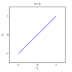
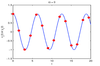
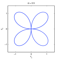
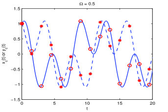
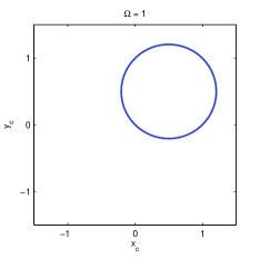
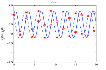
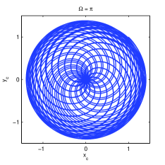
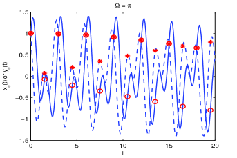
Fig. 3: Results for $\gamma_{x}=\gamma_{y}=1$. Left: trajectory of the center of mass, ${\bf x}_{c}(t)=(x_{c}(t),y_{c}(t))^{T}$ for $0\leq t\leq 100$. Right: coordinates of the trajectory ${\bf x}_{c}(t)$ (solid line: $x_{c}(t)$, dashed line: $y_{c}(t)$) for different rotation speed $\Omega$, where the solid and dashed lines are obtained by directly simulating the GPE and ‘*’ and ‘o’ represent the solutions to the ODEs in Lemma 3.

In addition, our simulations show that the dynamics of the center of mass are independent of the interaction coefficients $\beta$ and $\eta$, which is consistent with Lemma 3.

  

  

  

  

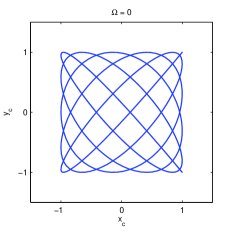
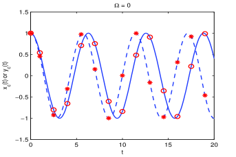
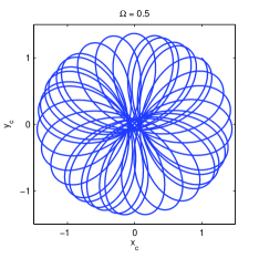
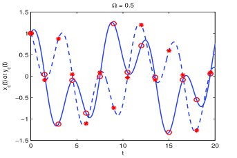
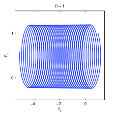
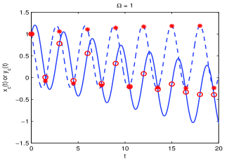
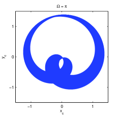
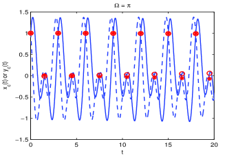
Fig. 4: Results for $\gamma_{x}=1,\gamma_{y}=1.1$. Left: trajectory of the center of mass, ${\bf x}_{c}(t)=(x_{c}(t),y_{c}(t))^{T}$ for $0\leq t\leq 100$. Right: coordinates of the trajectory ${\bf x}_{c}(t)$ (solid line: $x_{c}(t)$, dashed line: $y_{c}(t)$) for different rotation speed $\Omega$, where the solid and dashed lines are obtained by directly simulating the GPE and ‘*’ and ‘o’ represent the solutions to the ODEs in Lemma 3.

5.3 Dynamics of angular momentum expectation and condensate widths

To study the dynamics of the angular momentum expectation and condensate widths, we adapt the GPE (1.14)–(1.15) in 2D with SDM long-range interaction (1.13) and harmonic potential (1.19), i.e. we take $d=2$ and $\Omega=0.7$. Similarly, the initial condition in (1.18) is taken as

(5.3) $$\psi_{0}({\bf x})=\alpha\,\zeta({\bf x}),\qquad{\bf x}\in{\mathcal{D}},$$

where $\zeta({\bf x})$ is defined in (5.2) and $\alpha$ is a constant such that $\|\psi_{0}\|^{2}=1$. In our simulations, we consider the following four cases:

1. $\gamma_{x}=\gamma_{y}=1$, $\beta=25\sqrt{{10}/{\pi}}$, $\eta=0$, and ${\bf n}=(1,0,0)^{T}$;

2. $\gamma_{x}=\gamma_{y}=1$, $\beta=25\sqrt{{10}/{\pi}}$, $\eta=-15$, and ${\bf n}=(1,0,0)^{T}$;

3. $\gamma_{x}=\gamma_{y}=1$, $\beta=55\sqrt{{10}/{\pi}}$, $\eta=-15$, and ${\bf n}=(0,0,1)^{T}$;

4. $\gamma_{x}=1$, $\gamma_{y}=1.1$, $\beta=55\sqrt{{10}/{\pi}}$, $\eta=-15$, and ${\bf n}=(0,0,1)^{T}$.

 

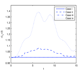
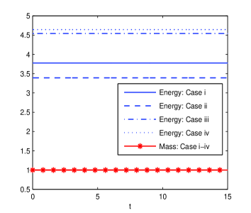
Fig. 5: Time evolution of the angular momentum expectation (left) and energy and mass (right) for Cases (i)-(iv) in section 5.3.

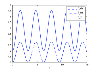
i) ii)

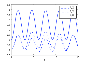
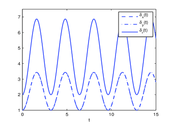
iii) iv)

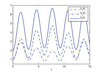
Fig. 6: Time evolution of condensate widths in the Cases (i)–(iv) in section 5.3.

In Figure 5, we present the dynamics of the angular momentum expectation, energy and mass for each of the above four cases in the interval $t\in[0,15]$. We see that if the external trap is radially symmetric in 2D, then the angular momentum expectation is conserved when either there is no dipolar interaction (Case (i)) or the dipolar axis is parallel to the $z$-axis (Case (iii)). Otherwise, the angular momentum expectation is not conserved. The above numerical observations are consistent with the analytical results obtained in Lemma 1. In addition, we find that our method conserves the energy and mass very well during the dynamics (cf. Fig. 5 right). Furthermore, from our additional numerical results not shown here for brevity, we observed that the angular momentum expectation is conserved in 3D for any initial data if the external trap is cylindrically symmetric and either there is no dipolar interaction or the dipolar axis is parallel to the $z$-axis, which can also be justified mathematically.

The dynamics of the condensate widths are presented in Figure 6. We find that $\delta_{r}(t)$ is periodic as long as the trapping frequencies satisfy $\gamma_{x}=\gamma_{y}$ and the influence of the dipole axis vanishes, e.g. in the Case (i), which confirms the analytical results of Lemma 2. Furthermore, from our additional numerical results not shown here for brevity, we observed that $\delta_{r}(t)$ is periodic and $\delta_{x}(t)=\delta_{y}(t)=\frac{1}{2}\delta_{r}(t)$ if $\eta=0$ for any initial data or ${\bf n}=(0,0,1)^{T}$ for radially symmetric or central vortex-type initial data.

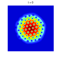
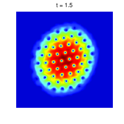
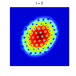
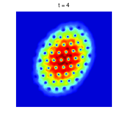
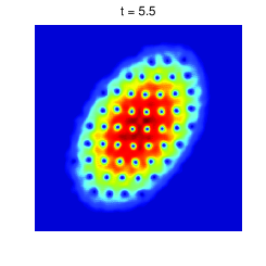
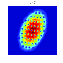
Fig. 7: Contour plots of the density function $|\psi({\bf x},t)|^{2}$ for dynamics of a vortex lattice in a rotating BEC (Case (i)). Domain displayed: $(x,y)\in[-13,13]^{2}$.

5.4 Dynamics of quantized vortex lattices

In the following, we apply our numerical method to study the dynamics of quantized vortex lattices in rotating dipolar BECs. Again, we adapt the GPE (1.14)–(1.15) in 2D with SDM long-range interaction (1.13) and harmonic potential (1.19), i.e. we choose $d=2$, $\beta=1000$ and $\Omega=0.9$. The initial datum in (1.18) is chosen as a stationary vortex lattice which is computed numerically by using the method in [49, 50] with the above parameters and $\gamma_{x}=\gamma_{y}=1$, $\eta=0$, i.e. no long-range dipole-dipole interaction initially. Then the dynamics of vortex lattices are studied in two cases:

1. perturb the external potential by setting $\gamma_{x}=1.05$ and $\gamma_{y}=0.95$ at $t=0$;

2. turn on the dipolar interactions by setting $\eta=-600$ and dipolar axis ${\bf n}=(1,0,0)^{T}$ at time $t=0$.

In our simulations, we use ${\mathcal{D}}=[-16,16]^{2}$, $\Delta{\widetilde{x}}=\Delta{\widetilde{y}}=1/16$ and $\Delta t=0.0001$. Figures 7–8 show the contour plots of the density function $|\psi({\bf x},t)|^{2}$ at different time steps for Cases (i) and (ii), respectively, where the wave function $\psi({\bf x},t)$ is obtained from $\phi(\widetilde{\bf x},t)$ by using interpolation via sine basis (see Remark 4.1). We see that during the dynamics, the number of vortices is conserved in both cases. The lattices rotate to form different patterns because of the anisotropic external potential and dipolar interaction in Cases (i) and (ii), respectively. In addition, the results in Case (i) are similar to those obtained in [10], where a spectral type method in polar coordinates was used to simulate the dynamics of vortex lattices.

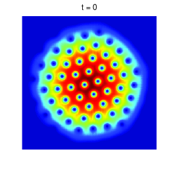
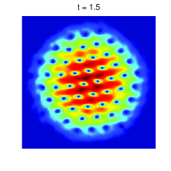
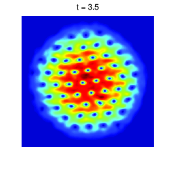
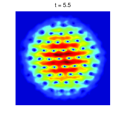
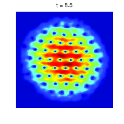
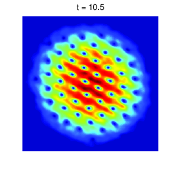
Fig. 8: Contour plots of the density function $|\psi({\bf x},t)|^{2}$ for dynamics of a vortex lattice in a rotating dipolar BEC (Case (ii)). Domain displayed: $(x,y)\in[-10,10]^{2}$.

6 Conclusions

We proposed a simple and efficient numerical method to simulate the dynamics of rotating dipolar Bose-Einstein condensation (BEC) whose properties are described by the Gross–Pitaevskii equation (GPE) with both the angular rotation term and the long-range dipole-dipole interaction. First, by decoupling the short-range and long-range interactions, we reformulate the GPE as a Gross-Pitaevskii-(fractional) Poisson system. Then we eliminate the angular rotation term from the GPE using a rotating Lagrangian coordinate transformation, which makes it possible to design a simple and efficient numerical method. In the new rotating Lagrangian coordinates, we presented a numerical method which combines the time-splitting techniques with Fourier/sine pseudospectral approximation to simulate the dynamics of rotating dipolar BECs. The numerical methods is explicit, unconditional stable, spectral accurate in space and second order accurate in time, and conserves the mass in the discretized level. The memory cost is $O(MK)$ in 2D and $O(MKL)$ in 3D, and the computational cost per time step is $O\left(MK\ln(MK)\right)$ in 2D and $O\left(MKL\ln(MKL)\right)$ in 3D. More specifically, the method is very easy to be implemented via FFT or DST. We then numerically examine the conservation of the angular momentum expectation and study the dynamics of condensate widths and center of mass for different angular velocities. In addition, the dynamics of vortex lattice in rotating dipolar BEC are investigated. Numerical studies show that our method is very effective in simulating the dynamics of rotating dipolar BECs.

Acknowledgement We acknowledge Professor Christof Sparber for stimulating and helpful discussions. Part of this work was done when the authors were visiting the Institute for Mathematical Sciences at the National University of Singapore in 2012.

References

- [1] M. Abad, M. Guilleumas, R. Mayol, M. Pi and D. M. Jazek, Vortices in Bose–Einstein condensates with dominant dipolar interactions, Phys. Rev. A, 79 (2009), article 063622.
- [2] J. R. Abo-Shaeer, C. Raman, J. M. Vogels and W. Ketterle, Observation of vortex lattices in Bose-Einstein Condensates, Science, 292 (2001), pp. 476–479.
- [3] A. Aftalion and Q. Du, Vortices in a rotating Bose–Einstein condensate: Critical angular velocities and energy diagrams in the Thomas–Fermi regime, Phys. Rev. A, 64 (2001), article 063603.
- [4] M. H. Anderson, J. R. Ensher, M. R. Matthewa, C. E. Wieman and E. A. Cornell, Observation of Bose-Einstein condensation in a dilute atomic vapor, Science, 269 (1995), pp. 198–201.
- [5] P. Antonelli, D. Marahrens and C. Sparber, On the Cauchy problem for nonlinear Schrödinger equations with rotation, Disc. Contin. Dyn. Syst. A, 32 (2012), pp. 703–715.
- [6] W. Bao, N. Ben Abdallah and Y. Cai, Gross-Pitaevskii-Poisson equations for dipolar Bose-Einstein condensate with anisotropic confinement, SIAM J. Math. Anal., 44 (2012), pp. 1713-1741.
- [7] W. Bao and Y. Cai, Mathematical theory and numerical methods for Bose-Einstein condensation, Kinet. Relat. Mod., 6 (2013), pp. 1-135.
- [8] W. Bao and Y. Cai, Optimal error estimates of finite difference methods for the Gross-Pitaevskii equation with angular momentum rotation, Math. Comp., 82 (2013), pp. 99-128.
- [9] W. Bao, Y. Cai and H. Wang, Efficient numerical methods for computing ground states and dynamics of dipolar Bose-Einstein condensates, J. Comput. Phys., 229 (2010), pp. 7874-7892.
- [10] W. Bao, Q. Du and Y. Zhang, Dynamics of rotating Bose-Einstein condensates and its efficient and accurate numerical computation, SIAM J. Appl. Math., 66 (2006), pp. 758-786.
- [11] W. Bao, D. Jaksch and P. A. Markowich, Numerical solution of the Gross–Pitaevskii equation for Bose–Einstein condensation, J. Comput. Phys., 187 (2003), pp. 318–342.
- [12] W. Bao, H. Li and J. Shen, A generalized Laguerre-Foruier-Hermite pseudospectral method for computing the dynamics of rotating Bose–Einstein condensates, SIAM J. Sci. Comput., 31 (2009), pp. 3685-3711.
- [13] W. Bao and H. Wang, An efficient and spectrally accurate numerical method for computing dynamics of rotating Bose–Einstein condensates, J. Comput. Phys., 271 (2006), pp. 612-626.
- [14] W. Bao and Y. Zhang, Dynamics of the ground state and central vortex state in Bose–Einstein condensation, Math. Mod. Meth. Appl. Sci., 15 (2005), pp. 1863-1896.
- [15] P. B. Blakie, C. Ticknor, A. S. Bradley, A. M. Martin, M. J. Davis and Y. Kawaguchi, Numerical method for evolving the dipolar projected Gross–Pitaevskii equation, Phy. Rev. E, 80 (2009), article 016703.
- [16] J. P. Boyd, A fast algorithm for Chebyshev, Fourier, and sinc interpolation onto an irregular grid, J. Comput. Phys., 103 (1992), pp. 243–257.
- [17] C. C. Bradley, C. A. Sackett, J. J. Tollett and R. G. Hulet, Evidence of Bose-Einstein condensation in an atomic gas with attractive interaction, Phys. Rev. Lett., 75 (1995), pp. 1687–1690.
- [18] V. Bretin, S. Stock, Y. Seurin and J. Dalibard, Fast rotation of a Bose-Einstein condensate, Phys. Rev. Lett., 92 (2004), article 050403.
- [19] Y. Cai, M. Rosenkranz, Z. Lei and W. Bao, Mean-field regime of trapped dipolar Bose-Einstein condensates in one and two dimensions, Phys. Rev. A, 82 (2010), article 043623.
- [20] M. M. Cerimele, M. L. Chiofalo, F. Pistella, S. Succi and M. P. Tosi, Numerical solution of the Gross–Pitaevskii equation using an explicit finite-difference scheme: An application to trapped Bose–Einstein condensates, Phys. Rev. E, 62 (2000), pp. 1382–1389.
- [21] N. R. Cooper, E. H. Rezayi and S. H. Simon, Vortex lattices in rotating atomic Bose gases with dipolar interactions, Phys. Rev. Lett., 95 (2005), article 200402.
- [22] K. B. Davis, M. O. Mewes, M. R. Andrews, N. J. van Druten, D. S. Durfee, D. M. Kurn and W. Ketterle, Bose-Einstein condensation in a gas of sodium atoms, Phys. Rev. Lett., 75 (1995), pp. 3969–3973.
- [23] J. J. García-Ripoll, V. M. Pérez-García and V. Vekslerchik, Construction of exact solution by spatial translations in inhomogeneous nonlinear Schrödinger equations, Phys. Rev. E, 64 (2001), article 056602.
- [24] R. Glowinski and P. Le Tallec, Augmented Lagrangian and operator splitting methods in nonlinear mechanics, SIAM Stud. Appl. Math., 9 (1989) SIAM, Philadelphia.
- [25] K. Góral, K. Rzayewski and T. Pfau, Bose–Einstein condensation with magnetic dipole-dipole forces, Phys. Rev. A, 61 (2000), article 051601(R).
- [26] A. Griesmaier, J. Werner, S. Hensler, J. Stuhler and T. Pfau, Bose–Einstein condensation of Chromium, Phys. Rev. Lett., 94 (2005), article 160401.
- [27] M. Hintermüller, D. Marahrens, P. Markowich, C. Sparber, Optimal bilinear control of Gross-Pitaevskii equations, arXiv:1202.2306 (2012).
- [28] K. Kasamatsu, M. Tsubota and M. Ueda, Nonlinear dynamics of vortex lattice formation in a rotating Bose–Einstein condensate, Phys. Rev. A, 67 (2003), article 033610.
- [29] S. Komineas and N.R. Cooper, Vortex lattices in Bose–Einstein condensates with dipolar interactions beyond the weak-interaction limit, Phys. Rev. A, 75 (2007), 023623.
- [30] R. K. Kumar and P. Muruganandam, Vortex dynamics of rotating dipolar Bose–Einstein condensates, J. Phys. B: At. Mol. Opt. Phys., 45 (2012), article 215301.
- [31] T. Lahaye, C. Menotti, L. Santos, M. Lewenstein and T. Pfau, The physics of dipolar bosonic quantum gases, Rep. Prog. Phys., 72 (2009), 126401.
- [32] M. Lu, N. Q. Burdick, S. H. Youn and B. L. Lev, Strongly dipolar Bose–Einstein condensate of Dysprosium, Phys. Rev. Lett., 107 (2011), article 190401.
- [33] K. W. Madison, F. Chevy, W. Wohlleben and J. Dalibard, Vortex formation in a stirred Bose–Einstein condensate, Phys. Rev. Lett., 84 (2000), pp. 806–809.
- [34] K. W. Madison, F. Chevy, V. Bretin and J. Dalibard, Stationary states of a rotating Bose–Einstein condensates: Routes to vortex nucleation, Phys. Rev. Lett., 86 (2001), pp. 4443–4446.
- [35] F. Malet, T. Kristensen, S. M. Reimann and G. M. Kavoulakis, Rotational properties of dipolar Bose–Einstein condensates confined in anisotropic harmonic potential, Phys. Rev. A, 83 (2011), article 033628.
- [36] M. R. Matthews, B. P. Anderson, P. C. Haljan, D. S. Hall, C. E. Wiemann and E. A. Cornell, Vortices in a Bose–Einstein condensate, Phys. Rev. Lett., 83 (1999), pp. 2498–2501.
- [37] P. Muruganandam and S.K. Adhikari, Fortran programs for the time-dependent Gross–Pitaevskii equation in a fully anisotropic trap, Comput. Phys. Commun., 180 (2009), pp. 1888–1912.
- [38] C. Raman, J. R. Abo-Shaeer, J. M. Vogels, K. Xu and W. Ketterle, Vortex nucleation in a stirred Bose–Einstein condensate, Phys. Rev. Lett., 87 (2001), article 210402.
- [39] S. Ronen, D. C. E. Bortolotti and J. L. Bohn, Bogoliubov modes of a dipolar condensate in a cylindrical trap, Phys. Rev. A 74 (2006), article 013623.
- [40] R. Seiringer, Ground state asymptotics of a dilute rotating gas, J. Phys. A: Math. Gen., 36 (2003), pp. 9755-9778.
- [41] J. Shen, T. Tang and L. Wang, Spectral Methods: Algorithms, Analysis and Applications, Springer, 2011.
- [42] G. Strang, On the construction and comparision of difference schemes, SIAM J. Numer. Anal., 5 (1968), 505-517.
- [43] R. P. Tiwari and A. Shukla, A basis-set based Fortran program to solve the Gross–Pitaevskii equation for dilute Bose gases in harmonic and anharmonic traps, Comput. Phys. Commun., 174 (2006), pp. 966-982.
- [44] M. Tsubota, K. Kasamatsu and M. Ueda, Vortex lattice formation in a rotating Bose-Einstein condensate, Phys. Rev. A 65 (2002), article 023603.
- [45] R. M. W. van Bijnen, A. J. Dow, D. H. J. O’Dell, N. G. Parker and A. M. Martin, Exact solutions and stability of rotating dipolar Bose–Einstein condensates in the Thomas–Fermi limit, Phys. Rev. A, 80 (2009), article 033617.
- [46] B. Xiong, J. Gong, H. Pu, W. Bao and B. Li, Symmetry breaking and self-trapping of a dipolar Bose-Einstein condensate in a double-well potential, Phys. Rev. A, 79 (2009), article 013626.
- [47] S. Yi and H. Pu, Vortex structures in dipolar condensates, Phys. Rev. A, 73 (2006), article 061602(R).
- [48] C. Yuce and Z. Oztas, Off-axis vortex in a rotating dipolar Bose–Einstein condensate, J. Phys. B: At. Mol. Opt. Phys., 43 (2010), article 135301.
- [49] R. Zeng and Y. Zhang, Efficiently computing vortex lattices in fast rotating Bose–Einstein condensates, Comput. Phys. Commun., 180 (2009), pp. 854–860.
- [50] Y. Zhang, Numerical study of vortex interactions in Bose–Einstein condensation, Commun. Comput. Phys., 8 (2010), pp. 327–350.
- [51] Y. Zhang and W. Bao, Dynamics of the center of mass in rotating Bose-Einstein condensates, Appl. Numer. Math., 57 (2007), pp. 697–709.
- [52] J. Zhang and H. Zhai, Vortex lattices in planar Bose-Einstein condensates with dipolar interactions, Phys. Rev. Lett., 95 (2005), article 200403.