Mixing, entropy and competition

Abstract

Non-traditional thermodynamics, applied to random behaviour associated with turbulence, mixing and competition, is reviewed and analysed. Competitive mixing represents a general framework for the study of generic properties of competitive systems and can be used to model a wide class of non-equilibrium phenomena ranging from turbulent premixed flames and invasion waves to complex competitive systems. We demonstrate consistency of the general principles of competition with thermodynamic description, review and analyse the related entropy concepts and introduce the corresponding competitive H-theorem. A competitive system can be characterised by a thermodynamic quantity — competitive potential — which determines the likely direction of evolution of the system. Contested resources tend to move between systems from lower to higher values of the competitive potential. There is, however, an important difference between conventional thermodynamics and competitive thermodynamics. While conventional thermodynamics is constrained by its zeroth law and is fundamentally transitive, the transitivity of competitive thermodynamics depends on the transitivity of the competition rules. Intransitivities are common in the real world and are responsible for complex behaviour in competitive systems.

This work follows the ideas and methods that are originated in analysis of turbulent combustion but reviews a much broader scope of issues linked to mixing and competition, including thermodynamic characterisation of complex competitive systems with self-organisation. The approach presented here is interdisciplinary and is addressed to a general educated reader, while the mathematical details can be found in the Appendices.

———————————–

Published: Phys. Scr. 85 (2012) 068201 (29pp)

1 Introduction

Thermodynamics allows for a concise description of complex stochastic systems, determining an overall trend behind a large number of random events and offering insightful generalisations. The success of classical thermodynamics is largely based on recognising and postulating irreversibility of the surrounding world that on one hand represents an obvious fact and on the other hand still awaits explanation from the first principles of physics. The second law of thermodynamics, which predicts irreversible increase of entropy — the key thermodynamic quantity serving as a measure of chaotic uncertainty — is equally applicable to a small combustor and to stars and galaxies.

This remarkable success of thermodynamics can not hide from us its major difficulty - our world appears to be much more complicated and much less chaotic than generally might be inferred from the second law. It is well known that complex non-equilibrium stochastic processes tend to display a significant level of regularity along with randomness [1]. In non-equilibrium phenomena, the production of physical entropy is typically high, in perfect agreement with the laws of thermodynamic. Although no direct violation of the laws of thermodynamics is known, thermodynamics struggles to explain complexity, which is often observed in essentially non-equilibrium phenomena: turbulent mixing and combustion as well as evolution of life forms may serve as typical examples. The entropy of turbulent fluctuations does not seem to be maximal and the same applies to entropies characterising distributions in other complex non-equilibrium processes. These entropies have similarities with but are not the same as the molecular entropy, which characterises disorder of molecular movements and is subject to the laws of thermodynamics. We use the term apparent entropy to distinguish entropy-like quantities from the molecular entropy.

The present work reviews the use of entropy in the analysis of turbulence, turbulent mixing and combustion and shows that the term “entropy” is commonly used to denote both apparent entropy and molecular entropy. The same trend can be observed across other disciplines. In principle, the use of apparent entropy may or may not imply the existence of underlying thermodynamics. The existence of apparent thermodynamics associated with mixing is of prime interest for this work. Thermodynamic description is a very general methodology involving abstract theories, i.e. theories not directly linked to the dynamics of molecules. The general theory of Gibbs measures [2] and the axiomatic thermodynamic theory [3], introducing entropy on the basis of ordering of thermodynamic states by Caratheodory’s adiabatic accessibility [4], should be mentioned in this respect.

Competitive systems, which are typically associated with complex stochastic behaviour, are common in the real world. Abstract competition, which studies generic principles of competition in their most abstract form, can be interpreted as a form of mixing [5]. This mixing, which is called competitive mixing, can be used to characterise various processes: turbulent combustion, invasion waves and other related phenomena [6]. Unlike conventional conservative mixing, competitive mixing can display complex behaviour with sophisticated interdependencies. After reviewing existing publications and taking into account a number of theorems presented in the Appendices, we demonstrate that competitive systems do allow for a thermodynamic description. The implications of this demonstration are profound: the evolution of competitive systems occurs in a stochastic manner but in agreement with competitive thermodynamics. A competitive system can be characterised by competitive entropy and by a new thermodynamic quantity — the competitive potential — which determines the likely direction of evolution of the system and is analogous to chemical potential in conventional thermodynamics (taken with the opposite sign). Following in the footsteps of classical thermodynamics, competitive thermodynamics recognises the obvious trend towards more competitive states while the details of the mechanism behind the competition rules may remain unknown.

Competitive thermodynamics, while answering many existing questions, poses several new ones. A conventional thermodynamic system evolves towards equilibrium and, once the global equilibrium is reached remains in this state indefinitely. Competitive systems tend to display much more complex and unending pattern of evolution — how this can be consistent with a thermodynamic description? The answer lies in the details. Competitive thermodynamics has a principal difference with conventional thermodynamics: transitivity of competitive thermodynamics can not be taken for granted. While conventional thermodynamics is constrained by its zeroth law and is fundamentally transitive, the transitivity of competitive thermodynamics depends on the transitivity of the competition rules. Intransitivities are not only possible in real competitive systems, but seem to be quite common. Unlike chemical potential or temperature, which can be assigned absolute values, the competitive potential becomes relative and this removes the rigid constraints of conventional thermodynamics and introduces complex patens into evolution. Intransitivity, which has long been known in science under the name of the Condorcet paradox [7] and has traditionally been considered as something paradoxical, abnormal or unwanted, is viewed here as a common property of nature.

The approach presented here is derived from the long-standing tradition of modelling turbulent reacting flows repeatedly reviewed in publications [8, 9, 10, 11, 12, 13, 14, 15, 16, 17, 18]. The rapid development over the last few decades of computational models designed for the simulation of transport, reaction and dispersion in turbulent flows has led to a wide use of Pope particles [8, 19]. These notional particles move in physical space and posses a set of properties that can be changed due to 1) kinetic evolution within each particle and 2) mixing exchanges between the particles. With the introduction of competitive mixing, Pope particles can be viewed not only as being effective tools for modelling of turbulent reacting flows but also as universal building blocks for a wide class of models that can simulate complex behaviour. Conventional conservative mixing does not result in significant stochastic interdependencies between the particles and a system of many particles can be characterised by a single one-particle pdf. If conventional mixing is replaced by competitive mixing, these interdependencies may become significant, dramatically increasing the effective dimensionality and complexity of the simulations. Competitive mixing naturally appears in simulations of turbulent premixed flames [6], which are driven by the forces of conventional thermodynamics. We review these applications and take the logical step of extending these thermodynamic descriptions to more complex competitive systems. There is a large number of publications dedicated to different aspects of complexity, for example, algorithmic (Kolmogorov-Chaitin) complexity and algorithmic entropy [20], complex adaptive systems (CAS) [21, 22] and evolution of complexity [23].

The phenomena we consider display a combination of chaotic and ordered behaviour. Entropy, which is conventionally used to characterise the balance of order and disorder, has been repeatedly applied to the analysis of non-equilibrium systems in general [24, 25, 26, 27, 28, 29] and turbulent flows in particular [30, 31, 32, 33, 34, 35, 36]. Our treatment of non-equilibrium processes is based on introducing non-conventional or apparent thermodynamics, which is not analogous to but still may have some links with the principles of non-equilibrium thermodynamics (i.e. entropy production principles of Prigogine [24] and Ziegler [26] and the fluctuation theorem [27]). This work follows the application of the concept of entropy to semi-autonomous elements, which in most cases can be effectively represented by Pope particles.

In accordance with the “Turbulent Mixing and Beyond” tradition, the review starts from the methods used in modelling of turbulent mixing and combustion and then extends these methods beyond turbulence to mixing and competitive systems of a general nature. The possibility of thermodynamic description is sought and, in many cases, found for these systems. While the thermodynamic description of mixing, both conservative and competitive, is the focus of the present work, the other areas are covered as necessary but only to the extent of their relevance to the main topic.

The review is divided into 8 sections and 4 appendices. The sections present the following material:

• Section 2 defines entropy for systems of notional particles. The defined entropy involves two major components: configurational (related to collective particle disorder) and potential (related to the state of each particle). The use of particle entropy in context of turbulent flows is subsequently reviewed.

• Section 3 analyses the effect of conservative and competitive mixing on entropy. Conventional conservative mixing models, which are commonly used in modelling of transport and reactions in turbulent flows, are reviewed and the condition that enforces conservative mixing to be entropy-consistent is presented. The conventional entropy of premixed combustion is extended (as apparent entropy) to become a common property of systems involving competitive mixing.

• Section 4 explores the fundamental link between ordering, ranking and entropy. The analysis is directed at competitive mixing but the related methodologies developed in other disciplines (adiabatic accessibility and economic utility) are also reviewed.

• Section 5 analyses the behavior of systems with transitive competition and shows that it is thermodynamically consistent. The thermodynamic analogy is especially strong for the class of mutations that is called Gibbs mutations by analogy with Gibbs measures. A transitive competitive system tend to promptly reach a quasi-equilibrium state and then slowly drift in the direction of increasing competitiveness. Both processes are characterised by increase in apparent entropy.

• Section 6 investigates a more complex case of intransitive competition. Thermodynamic considerations can be applicable if intransitive competition retains some transitive properties. The applicability of competitive thermodynamics to general intransitive systems, which may involve competitive cooperation and other forms of complex behaviour, is also explored.

• Section 7 gives several examples of intransitive behaviour including intransitivity in turbulent flows, in chemical reactions and in a generic competitive system displaying complex behaviour.

• Section 8 outlines the main conclusions for this work.

• Apendices present useful mathematical details and additional material, which is not available in the published literature but is essential to this review:

  • Appendix A gives a brief summary of the related mathematical results.

  • Appendix B generalises rankings for preferential mixing

  • Appendix C introduces Gibbs and near-Gibbs mutations and explores their relations with Markov processes, Gibbs measures and the fluctuation theorem.

  • Appendix D presents governing equations, general theorems and analysis of some special cases for evolution of competitive systems.

2 Entropy of particle systems

Although entropy was introduced in thermodynamics and statistical physics by Clausius, Boltzmann and Gibbs as a specific, heat-related property of large systems of molecules, the modern use of this term ranges from rigorous extensions of the concept of entropy (such as Shannon’s entropy in information theory) to relatively vague and intuitive interpretations (such as social entropy). The more general view of entropy, which takes its origin in Shannon’s famous work [37], sees entropy as a property characterising disorder of stochastic behaviour in general. In the present we understand entropy as a quantity which displays (or is expected to display) behavior similar to that of the molecular entropy. This entropy, though, does not necessarily coincide with the molecular entropy used in conventional thermodynamics and the word apparent is used whenever it is necessary to stress this difference. Thermodynamic quantities introduced for competitive systems can be also named as competitive. In this section, common definitions of entropy for a system of notional particles are considered.

2.1 Configurational entropy and potential entropy

Consider $n$ notional stochastic particles, where each of these particle is characterised by a vector $\mathbf{X}=(X^{(1)},...,X^{(k_{d})}).$ The joint probability distribution of these particles is denoted by $P_{n}=P_{n}(\mathbf{X}_{1},...,\mathbf{X}_{n})$. The Gibbs entropy is introduced as a statistical sum (or integral) over all possible states of this system

$$\bar{S}=\int_{\infty}\left(-P_{n}\ln\left(\frac{P_{n}}{A_{n}}\right)+P_{n}s_{n}\right)d\mathbf{X}_{1}...d\mathbf{X}_{n},$$ (1)

where $A_{n}$ can be interpreted as a priori statistical weight characterising effective volumes in the parameter space. This definition is conventional [33] but includes an additional term $P_{n}s_{n},$ which is considered below. If the particles are (or can be treated as) statistically independent then the joint pdf (probability density function) is decomposed into single-particle pdfs

$$P_{n}=P_{n}(\mathbf{X}_{1},...,\mathbf{X}_{n})=P(\mathbf{X}_{1})...P(\mathbf{X}_{n}),$$ (2)

and the equation for entropy takes the form of Boltzmann entropy

$$\bar{S}=\;\underset{\bar{S}_{c}}{\underbrace{-n\int_{\infty}P(\mathbf{X})\ln\left(\frac{P(\mathbf{X})}{A(\mathbf{X})}\right)d\mathbf{X}}}\;+\;\underset{\bar{S}_{f}}{\underbrace{n\int_{\infty}P(\mathbf{X})s(\mathbf{X})d\mathbf{X}}}$$ (3)

The first term $\bar{S}_{c},$ which is called here configurational entropy, is related to the stochastic nature of the particles distribution while the second term $\bar{S}_{f}$, which is called potential entropy, is related to the particle state and characterised by the entropy potential $s(\mathbf{X})$. If we interpret the particles as computational objects, the configurational entropy is the same as Shannon entropy of variable $\mathbf{X}$. It is arguable that, if the particles are not distinguishable, the value $\ln(n!)\approx n\ln(n)$ needs to be deducted from (3). This however does not affect our considerations since the number of particles is kept constant. The entropy $\bar{S}$ can be interpreted as free entropy, defined as $\bar{S}=-G/T$ where $G$ is the Gibbs (or Helmholtz) free energy and $T$ is the absolute temperature measured in energy units. In this case the physical interpretation of $s(\mathbf{X})$ is most transparent and linked to free energy of each state $\mathbf{X}$. The distinction between configurational and non-configurational free energies is commonly used in thermodynamic modelling [38]. In the present work, we do not restrict our consideration to a specific interpretation of $\bar{S}$. Inclusion of a priori statistical weight $A(\mathbf{X})$ makes the definition of entropy invariant with respect to replacements of variables $\mathbf{X}$.

The Gibbs entropy and Boltzmann entropy are equivalent only if the particles are independent. The particles may display some dependence in case of conventional conservative mixing [39] but these dependencies are typically small. As discussed in the following sections, complex particle behavior, which can be observed in the case of competitive mixing, may be accompanied by significant particle dependencies and substantial differences between the two definitions. In this case, however, Gibbs entropy becomes computationally intractable since the sum is to be evaluated over all alternative realizations in the overall composition space of very large dimension $n\times k_{d}.$ Typically, these alternative realizations remain unknown in computations while the whole ensemble of realisations may be difficult to define for complex systems. Our analysis is largely based on Boltzmann entropy, which is evaluated using the discrete representation of the single-particle pdf $P(\mathbf{X})$ by the current distribution of $n$ particles, where $n$ is assumed to be large. Note that in complex systems the current distribution may fluctuate even if $n$ is large.

2.2 Entropy of Pope particles

We now consider Pope particles and distinguish location of the particle denoted by $\mathbf{x}=(x_{1},...,x_{k_{x}})$ and particle properties denoted by $\mathbf{y}=(y_{1},...,y_{k_{y}}),$ that is $\mathbf{X}=(\mathbf{x},\mathbf{y})$ and $k_{d}=k_{x}+k_{y}$. The variables $x_{1},...,x_{k_{x}}$ represent physical coordinates and, possibly, other reference variables such as those used in MMC mixing [40, 41]. The coordinates $\mathbf{x}$ are conventionally governed by a Markov diffusion process while the particle properties $\mathbf{y}$ change due to mixing and, possibly, chemical reactions. With this distinction drawn between the physical coordinates $\mathbf{x}$ and particle properties $\mathbf{y,}$ we assume that entropy of the particle state $s$ is dependent on particle properties $\mathbf{y}$ but not on particle coordinates $\mathbf{x}$ (that is particles are not placed in any force field acting in physical space). The entropy can be divided into volumetric and local $S=S(\mathbf{x})$ components according to

$$\bar{S}=n\int_{\infty}\left(S(\mathbf{x})-\ln(p(\mathbf{x}))\right)p(\mathbf{x})d\mathbf{x}$$

$$S(\mathbf{x})=\int_{\infty}p(\mathbf{y|x})s(\mathbf{y})d\mathbf{y-}\int_{\infty}p(\mathbf{y|x})\ln\left(\frac{p(\mathbf{y|x})}{A(\mathbf{y,x})}\right)d\mathbf{y}\;$$

The one-particle pdf $P=P\left(\mathbf{y},\mathbf{x},t\right)$ governing distribution of Pope particles satisfies the equation [8, 39]

$$\frac{\partial P}{\partial t}+\mathop{\mathrm{d}iv}\left(\mathbf{v}P\right)-D\nabla^{2}P+\sum_{j}\frac{\partial W^{(j)}P}{\partial y^{(j)}}=\left[\frac{dP}{dt}\right]_{\mathop{\mathrm{m}ix}},$$ (4)

where $\mathbf{v}$ is the velocity in physical space $\mathbf{x}$, $D$ is the diffusion coefficient in physical space, $W^{(j)}$ is the reaction rate and the term on right hand side symbolically represents the effect of mixing. After some conventional manipulations, differentiating equation (3) results in

$$\frac{d\bar{S}}{dt}=n\underset{\infty}{\int\int}\left(\digamma_{x}+\sum_{j}\frac{\partial W^{(j)}}{\partial y^{(j)}}-\ln(P)\left[\frac{dP}{dt}\right]_{\mathop{\mathrm{m}ix}}\right)d\mathbf{x}d\mathbf{y+}$$

$$+n\underset{\infty}{\int\int}\left(P\sum_{j}W^{(j)}\frac{\partial s(\mathbf{y})}{\partial y^{(j)}}+s(\mathbf{y})\left[\frac{dP}{dt}\right]_{\mathop{\mathrm{m}ix}}\right)d\mathbf{y}d\mathbf{x,}$$ (5)

where

$$\digamma_{x}=P\mathop{\mathrm{d}iv}\left(\mathbf{v}\right)+D\frac{\left(\nabla P\right)^{2}}{P}$$

represents terms related to spatial inhomogeneity. The velocity divergence term was previously derived and investigated by Falkovich and Fouxon [33], who concluded that this term may result in entropy extraction from the system to the environment. The effect of the second term is well known – this term contributes to generation of entropy [42]. In the present work we focus on the mixing term and its influence on entropy and mainly restrict our attention to a spatially homogenous and non-reacting case. The mixing operator is typically presumed to be localised in $\mathbf{x}$-space and can be assumed to be non-preferential with respect to $\mathbf{y}$. That is all particles are selected for mixing from a given location $\mathbf{x}$ with equal probability irrespective of their properties. The simplest mixing models are non-preferential but, in principle, modelling can be improved by exercising proper preferences during mixing.

2.3 Maximal entropy distribution and competitive potential

In the rest of the paper we denote $P(\mathbf{y|x})=f(\mathbf{y})$ and consider only local characteristics so that the equation for the local entropy takes the form

$$S=\underset{S_{c}}{\;\underbrace{-\int_{\infty}f(\mathbf{y})\ln\left(\frac{f(\mathbf{y})}{A(\mathbf{y})}\right)d\mathbf{y}}}\;+\;\underset{S_{f}}{\underbrace{\int_{\infty}f(\mathbf{y})s(\mathbf{y})d\mathbf{y}}}$$ (6)

With the use of the equilibrium function $f_{0}(\mathbf{y})$ defined by

$$f_{0}(\mathbf{y})=\frac{A(\mathbf{y})}{Z}\exp\left(s(\mathbf{y})\right),$$ (7)

where

$$Z=\int_{\infty}A(\mathbf{y})\exp\left(s(\mathbf{y})\right)d\mathbf{y}$$ (8)

is the partition function, the entropy equation takes the form

$$S([f])\mathbf{=}\int_{\infty}f(\mathbf{y})\left(\ln(Z)-\ln\left(\frac{f(\mathbf{y})}{f_{0}(\mathbf{y})}\right)\right)d\mathbf{y}$$ (9)

The notation $S([f])$ is used to emphasise that $S$ is a functional of the distribution $f(\mathbf{y})$. Equation (9) is similar to the Kullback-Leibler divergence [43], that is known to achieve global entropy maximum

$$S([f_{0}])=\ln(Z)$$

by the distribution $f(\mathbf{y})=f_{0}(\mathbf{y})$.

For competitive systems, we also introduce competitive potential $\chi$ defined by

$$\chi(\mathbf{y})=\frac{\delta S}{\delta f(\mathbf{y})}=-\ln\left(\frac{f(\mathbf{y})}{f_{0}(\mathbf{y})}\right)+\chi_{0},$$ (10)

where

$$\chi_{0}=\ln(Z)-1$$ (11)

is the competitive potential of the equilibrium state. The constant of unity can be omitted from these equations. The a priori statistical weight $A(\mathbf{y})$ can be subject to different physical interpretations in competitive systems but it seems most logical to link $A(\mathbf{y})$ to the probability distributions assuming that competition is switched off (i.e. to the a priori probability). Particles with fixed $\mathbf{y}$ can be treated as reactants with potential $\chi$ while $\chi_{0}$ represents the potential of the system composed from different equilibrated reactants. Note that $f(\mathbf{y})$ should be multiplied by $n,$ if the number of particles $n$ may change. The competitive potential can be seen as a thermodynamic quantity which is similar to the chemical potential of reacting systems although $\chi$ is defined with the opposite sign. The sign of $\chi$ is selected to avoid a direct conflict with the common-sense interpretation of the expression of “having a high competitive potential”. This change in sign does not affect any physical properties of the system and is purely a notational matter. The similarity of competitive and chemical potentials is linked to the fact that it is the number of particles that is presumed to be preserved in interactions. Entropy combined with preservation of energy introduces the temperature. The particle systems considered here do not have temperature as long as there is no associated energy-like quantity that is conserved in mixing interactions.

2.4 Entropy in studies of turbulent flows.

In this section, we review the use of entropy in studies of turbulent flows revealing that different physical quantities or different conditions may in fact be implied when invoking this term. The molecular entropy has been used on numerous occasions to construct models of turbulent flows. The following examples indicate the wide scope of possible applications but, of course, are not intended as a comprehensive review of all possible applications. Molecular entropy can be used to characterise the spectrum of convective turbulence [44], ensure consistency of models with the laws of thermodynamics [45], control mixing processes [42], or model turbulent combustion [46]. In the last work [46], entropy is used in stochastic simulations as a convenient progress variable that allows for effective reduction of the chemical composition space [47].

Production of molecular entropy is the key factor in two general principles applicable to non-equilibrium dynamics: Prigogine’s theorem of minimal entropy production [24] and Ziegler’s maximal entropy production (MEP) principle [26]. Despite the apparent contradiction, these principles do not interfere with each other and both of the principles are consequences of Onsager’s reciprocal relations. Prigogine’s theorem is formulated for the specific conditions of a system asymptotically converging to steady (but not necessarily equilibrium) state where entropy production reaches its minimum while MEP is related to determining thermodynamic flows for given thermodynamic forces and at a fixed moment of time. According to a number of authors [25, 29], MEP can also be viewed as a very general principle: if a nonlinear system has several routes of moving towards its equilibrium state, nature seems to prefer the route with maximal entropy production. For example, turbulent flow is a more likely state than laminar flow and the former has higher dissipation and higher entropy production. This MEP principle seems to be very plausible and general but it still needs qualifications of conditions and justification [48]. Ozawa et al [49] analysed several different types of turbulent flows and concluded that MEP is applicable to these flows. The probabilities of positive and negative values of the entropy generation in non-equilibrium thermodynamics are connected by the fluctuation theorem [27], which indicates that entropy increases are much more likely than entropy reductions. The variational principles of non-equilibrium thermodynamics have been previously reviewed in the literature [28].

The possibility of applying the entropy concept to macroscopic motions in turbulence and other similar processes (rather than to thermodynamic microstates) is the main interest of the present work. Pope [30] suggested that in absence of any further information, the best way of approximating pdfs in turbulent flows is maximisation of entropy of the pdf constrained by available information about the pdf. Falkovich and Fouxon [33] analysed turbulence spectra with the use of entropy defined similar to the configurational entropy in the present work. Apparent thermodynamics is quite successful in specifying properties of inverse cascade in two-dimensional turbulence [87, 2005], since energy is preserved in this cascade and there is no vortex stretching in two dimensions. Dupree [31] analysed two-dimensional turbulence and introduced a definition of entropy which has two terms similar to configurational and state terms in equation (6). Three-dimensional turbulence, however, has proven to be more difficult and less susceptible to analysis based on the thermodynamic principles. Celani and Seminara [34] used DNS (direct numerical simulations) results to demonstrate that the statistics of turbulent scalar transport differs from the statistics expected in Gibbs equilibrium. Duplat and Villermaux [36] considered random stirring of a scalar field and found that it does not produce a field with maximal entropy. In all these works, fluctuations are treated as bringing additional chaos and entropy of these fluctuations is a positive quantity. Sancho and Llebot [32], however, suggest that the entropy associated with turbulent motion, which is more ordered as compared to highly chaotic molecular motion, is negative. This does not contradict the other publications since turbulent entropy is defined in Ref. [32] as the difference between the molecular entropy in a turbulent flow and that in a notional state of the flow after all turbulent fluctuations have been dissipated by viscosity. These examples illustrate that different quantities can be introduced as entropy and be very useful for analysis of non-equilibrium processes. However, when these quantities are different from the conventional molecular entropy, it is important to accurately define the quantity under consideration. In the present work, we use the term apparent entropy to distinguish entropy-like quantities from the molecular entropy. A similar distinction was drawn by Gray-Weale and Attard [35] who use the terms “first entropy” and “second entropy” to distinguish the quantities analogous to the molecular and apparent entropies. Unlike molecular entropy, the apparent entropy is not necessarily controlled by the laws of thermodynamics (separately from molecular entropy), and its properties require a special investigation.

3 Entropy and mixing

3.1 Entropy change by conservative mixing

In this subsection we consider how entropy is changed by mixing as simulated by the major conventional mixing models. Mixing between particles can be preferential, when particle properties affect the selection of particles for mixing, or non-preferential. Although all mixing models we consider perform mixing between particles locally in physical space $\mathbf{x}$, non-preferential mixing models do not discriminate particles on the basis of their properties $\mathbf{y}.$ In principle, preferential mixing allows for additional adjustment of mixing models to match better the physical mixing processes they simulate. Mixing preference can generally be expressed with the use of the mixing connectivity function $0\leq\Psi_{pq}\leq 1$ defined so that particles $p$ and $q$ can not mix if $\Psi_{pq}=0,$ particles $p$ and $q$ are most likely to be selected for mixing if $\Psi_{pq}=1.$ The example problem is conventional homogeneous mixing of two initial states with $y=0$ and $y=1$ occurring with equal probability into the final state of $y=1/2$.

The models commonly used in combustion applications include IEM (Interactions by Exchange with the Mean, [51]), the Curl’s [52] and modified Curl’s mixing models [53, 54], the EMST (Euclidean Minimal Spanning Tree) [55] and the MMC (Multiple Mapping Conditioning) model [40, 41]. The two last models represent stochastic versions of Mapping Closure (MC) [56] and, for the problem considered here, would perform similar to MC. EMST introduces MC-type mixing through preferential mixing between particles. MMC exercises preferential mixing between particles but only in terms of the special reference variables that are added to the set of physical coordinates $\mathbf{x}$; the selection of particles does not depend on $\mathbf{y}$ during MMC mixing. Mixing in the conventional Curl’s model is non-preferential.

Mixing affects both the configurational and state entropies. The change in configurational entropy is considered first. If the initial pdf $f(y)$ has Delta-functions, the IEM and the old Curl’s model do no produce smooth pdf distributions and are not suitable for this analysis. The mixing simulated by modified Curl’s model and MP results in smooth distributions for which the configurational entropy is well defined. The Curl’s model specifies mixing of particle $p$ with another particle $q$ by formula

$$\acute{y}_{p}=\frac{1+\eta}{2}y_{p}+\frac{1-\eta}{2}y_{q},$$ (12)

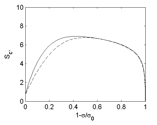
Figure 1: Evolution of configurational entropy $S_{c}$ in homogeneous turbulence simulated by mapping closure (solid line) and by modified Curl’s model (dotted line)

where the extent of mixing $\eta$ is constant for the old Curl’s model and random for the modified Curl’s model. We use a uniform distribution of $\eta$ on the interval $[0,1]$. The calculated values of the configurational entropy versus a time-like variable $1-\sigma/\sigma_{0}$ where $\sigma^{2}=\left\langle(y-\left\langle y\right\rangle)^{2}\right\rangle$ and $\sigma_{0}=\sigma(t_{0})$ are presented in Figure 1. There is a noticeable difference in entropies at the first stages of the mixing process that becomes small in the final stages of mixing despite the fact that MC-simulated pdf correctly approaches the Gaussian distribution while the pdf simulated by the modified curls model does not. The pdf simulated by MC is very close to the scalar pdf in real homogeneous turbulence [57] and so should be the configurational entropy term shown in Figure 1.

We note that the configurational entropy can both increase and decrease in simulations. This, of course, does not contradict to the second law of thermodynamics as the second component — the potential entropy — must be taken into account. For the case of ideal mixing the molecular entropy of mixing is defined by

$$s(y)=-\beta_{m}\left(y\ln(y)+(1-y)\ln(1-y)\right)$$ (13)

where the constant $\beta_{m}$ is introduced to account for Boltzmann constant and scale different entropies consistently. The term $s(y)$ enters equation (6) as the potential entropy $S_{f}$ . We can show that this quantity always increases when simulated by any mixing model producing a non-negative approximation for the conditional scalar dissipation $N_{y}=\left\langle D(\nabla y)^{2}|y\right\rangle$. Indeed the pdf scalar transport equation

$$\frac{\partial f(y)}{\partial t}=-\frac{\partial^{2}N_{y}f(y)}{\partial y^{2}}$$

results in the following expression for the entropy change

$$\frac{dS_{f}}{dt}=\int_{0}^{1}\frac{\partial f(y)}{\partial t}s(y)dy=$$

$$=-\int_{0}^{1}\frac{\partial^{2}N_{y}f(y)}{\partial y^{2}}s(y)dy=-\int_{0}^{1}N_{y}f(y)\frac{d^{2}s(y)}{dy^{2}}dy\geq 0$$ (14)

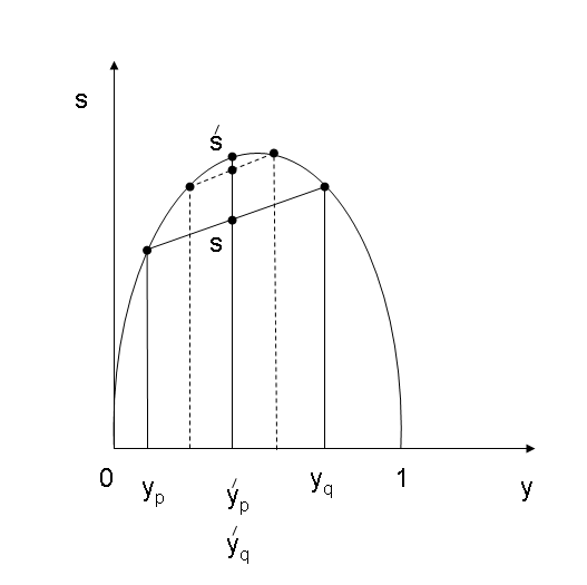
Figure 2: Change in entropy of mixing $s(y)$ induced by Curl’s mixing

considering the fact that $d^{2}s/dy^{2}$ is negative for $s(y)$ defined by (13). The integral is evaluated here by parts while taking into account that both $N_{y}f(y)$ and its derivative tend to zero at the boundaries $y=0$ and $y=1$ [12]. Figure 2 shows the curve $s(y)$ and demonstrates that after both complete and incomplete mixing of two particles $p$ and $q$ the mean entropy of these particles $(s(y_{p})+(y_{q}))/2$ increases.

This example illustrates the following important point. The total entropy can be treated as the conventional thermodynamic entropy with the potential entropy $S_{f}$ representing chaos of molecules completely mixed to molecular level and the configurational entropy $S_{c}$ representing the chaos of turbulent fluctuations. In this case, however, the term $S_{f}$ is proportional to the number of molecules and $\beta_{m}$ is so large that the term $S_{c}$ is indistinguishable in the sum. The entropy $S=S_{c}+S_{f}$ does, of course, satisfy the second law of thermodynamics. It can be very useful to consider the entropy of turbulent fluctuations but this quantity needs to be examined separately from the molecular entropy.

3.2 Entropy change by competitive mixing

Abstract competition studies the principles of competition in their most generic form [58]. The purpose of this representation may be seen to be similar to that of the Turing machine: making complex behaviours susceptible to general analysis but not specifically simulating any real devices or processes. Consider a complex system that has a large number of autonomous elements engaged in competition with each other. The evolution of a competitive system involves, in its general form, a process of determining a winner and a loser for competition between any two elements of the system. The properties of the loser are lost while the winner duplicates its properties into the resource previously occupied by the loser. The duplication process may involve random changes, which are customarily called mutations irrespective of the physical nature of the process. These mutations are predominantly negative or detrimental but can occasionally deliver a positive outcome. It is easy to see that abstract competition can be represented by a system of Pope particles, provided conventional conservative mixing is replaced by competitive mixing as discussed below. In context of computations, the competing elements or any other notional autonomous objects are conventionally called particles without implying a reference to physical particles of any kind. In the present review “elements” and “particles” are used synonymously with “elements” primarily referring to competing components of general nature and “particles” to their computational implementations.

Unlike conservative mixing, competitive mixing does not conserve the scalar values and gives a priority to the particle in a mixing group that is determined as the “winner” by duplicating its properties. The properties that belong to the loser are lost. The binary relationship “$\mathbf{y}_{p}$ stronger than $\mathbf{y}_{q}",$ or $\mathbf{y}_{p}\succ\mathbf{y}_{q},$ means that particle $p$ is the winner and particle $q$ is the loser in competition of these particles. If $\mathbf{y}_{p}$ is stronger than $\mathbf{y}_{q}$ (i.e. $\mathbf{y}_{p}\succ\mathbf{y}_{q}$) then, by definition, $\mathbf{y}_{q}$ is weaker than $\mathbf{y}_{p}$ (i.e. $\mathbf{y}_{q}\prec\mathbf{y}_{p}$). If $\mathbf{y}_{p}$ and $\mathbf{y}_{q}$ have the same strength then write $\mathbf{y}_{p}\simeq\mathbf{y}_{q},$ while “$\preccurlyeq$” implies “$\prec$” or “$\simeq$” and “$\succcurlyeq$” implies “$\succ$” or “$\simeq$”. The outcome of competition is determined by the properties of the particles. Although more complicated schemes can be considered, competitive mixing is introduced here according to the following mixing rules [5]

$$\mathbf{\acute{y}}_{p}=\left\{\begin{array}[]{ccc}\mathbf{y}_{q}+\mathbf{\zeta},&\mathbf{y}_{p}\prec\mathbf{y}_{q},R_{pq}=-1&(\mathop{\mathrm{l}oser})\\ \left[\begin{array}[]{c}\mathbf{y}_{q}+\mathbf{\zeta}\\ \mathbf{y}_{p}\end{array}\right],&\mathbf{y}_{p}\simeq\mathbf{y}_{q},R_{pq}=0&(\mathop{\mathrm{d}raw})\\ \mathbf{y}_{p},&\mathbf{y}_{p}\succ\mathbf{y}_{q},R_{pq}=+1&(\mathop{\mathrm{w}inner})\end{array}\right.,$$ (15)

where $R_{pq}=-R_{qp}$ is the antisymmetric competition index and $\mathbf{\zeta}$ represents random mutations. Although this term is obviously borrowed from biology, mutations used here represent random redistribution of resources (i.e. particles) between different states and should not be confused with genetic mutations. In the case of a draw, the two possible outcomes are selected with equal probability. In principle, particles $p$ and $q$ can also be isolated from each other $\mathbf{y}_{p}\parallel\mathbf{y}_{q},$ which corresponds to $\Psi_{pq}=0$; in this case $R_{pq}$ does not need to be defined but still can be defined for these particles if convenient. Competition can be illustrated by the following reaction between the particles

$$\mathbf{y}_{p}+\mathbf{y}_{q}+\mathop{\mathrm{e}nergy}\rightarrow\mathbf{y}_{p}+\mathbf{y}_{p}^{\prime},\;\;\;\;\mathbf{y}_{p}\succ\mathbf{y}_{q}$$ (16)

where $\mathbf{y}_{p}^{\prime}$ represents a mutated version of $\mathbf{y}_{p}$, $\mathbf{y}_{p}$ is stronger than $\mathbf{y}_{q}$ and the word “energy” indicates existence of an external source of energy.

The most simple example of competitive mixing is given by mixing of two states the losing state of $y=0$ and the winning state of $y=1.$ The properties of this mixing were investigated by Klimenko and Pope [6]. This mixing can be considered as a model for turbulent premixed combustion as well as for evolutionary invasion processes such as invasion of more successful species into the area occupied by less successful species. The model follows findings of Pope and Anand [59] that when reactions are fast the pdf of the reaction progress variable is dominated by two states: unburned $y=0$ and burned $y=1.$ The governing equation for this model is related to the KPP-Fisher equation [60, 61] and to the BML (Bray-Moss-Libby) model for premixed turbulent combustion [62]. The equation is named after Fisher who introduced it first and after Kolmogorov, Petrovsky and Piskunov who investigated the mathematical properties of this class of equations. For this case, the entropy equation (6) takes the form

$$S=\underset{S_{f}}{\underbrace{s_{1}\left\langle y\right\rangle}}\mathbf{-}\underset{S_{c}}{\underbrace{\mathbf{(}\left\langle y\right\rangle\ln\left(\left\langle y\right\rangle\right)+(1-\left\langle y\right\rangle)\ln((1-\left\langle y\right\rangle))}},$$ (17)

where we put $s(0)=0$ and $s_{1}=s(1)$ without loss of generality and $\left\langle y\right\rangle$ is the average value of $y$ over the two states $y=0$ and $y=1$. Although one may notice some similarity with equation (13), the physical meaning of that equation is different. As $\left\langle y\right\rangle$ increases due to mixing, configurational entropy $S_{c}$ increases but then, as the winning state becomes more and more dominant in the distribution, decreases. For combustion waves, this correspond to converting reactants into the products and $S_{c}=0$ when the reactions are complete and only products are present. The products have a much higher value of entropy than the reactants (i.e. $s_{1}\gg 1)$ and this ensures that the reactions are directed from reactants to the products.

The existence of thermodynamics driving chemical reactions towards their equilibrium states is obvious. Since the same model based on Pope particles can be used to simulate invasions [6], there should be an apparent thermodynamics, which can characterise the invasion and be similar to the conventional thermodynamics of the chemical reactions mentioned above. While noting the similarities between reactions and invasions, we should not forget about the differences. Reactions in premixed combustion are directly driven by conventional thermodynamics towards maximal molecular entropy (or possibly minimal molecular Gibbs/Helmholtz free energy). In this case apparent thermodynamics is directly linked to conventional thermodynamics. Molecular entropy of successful species is not necessarily higher than (and the Gibbs/Helmholtz free energy is not necessarily lower than) that of unsuccessful species and the apparent and molecular quantities are not directly linked. Competitive systems in this case must receive exergy from outside to avoid the constraints imposed by conventional thermodynamics on isolated systems. Positive values of the apparent entropy potential $s_{1}$ indicate the higher probability of presence of successful species in the equilibrium mixture irrespective of the physical reasons that ensure this success. While molecular thermodynamics explains the “success” of products over the reactants, it is not likely to offer a universal justification for the success of some competing elements over the others. Apparent thermodynamics recognises the obvious: nature has a greater affinity towards some states or competitive elements as compared to the other states or elements, irrespective whether we have an explanation for this affinity or not. Apparent thermodynamics is not fully reducible to molecular thermodynamics in the same way as molecular thermodynamics is not fully reducible to the laws of conventional and quantum mechanics.

The invasion process is redistribution of the available resources in favor of the successful species. Mutations represent randomness in this process and may or may not be related to genetic mutations. The relativistic nature of the competitiveness should be stressed. Weaker species are perfectly stable and become weak only in presence of stronger species in the same way as reactants disappear only when their transformation into products is allowed. We now proceed further to introduce a special thermodynamics that can characterise competitive systems.

4 Ordering, ranking and entropy

4.1 Ranking in competitive systems

Ranking of particles or elements in competition reflects how well a particle performs relative to the other particles. We distinguish the following rankings:

1. Two-particle ranking is the index function $R_{pq}=R(\mathbf{y}_{p},\mathbf{y}_{q})$ that determines the winner and the loser in competition of $p$ and $q$ as shown in equation (15)

2. Absolute ranking is a function $r_{\#}(\mathbf{y}_{p})$ that determines the outcomes of the competition by

   $$r_{\#}(\mathbf{y}_{p})\leq r_{\#}(\mathbf{y}_{q})\;\;\Leftrightarrow\;\;\mathbf{y}_{p}\preccurlyeq\mathbf{y}_{q}$$ (18)

   that is $r_{\#}(\mathbf{y}_{p})\leq r_{\#}(\mathbf{y}_{q})$ when and only when $q$ is not a loser in competition with $p.$ Introduction of absolute ranking requires transitivity and is subject to additional conditions as discussed in the following subsections.

3. Relative ranking $r(\mathbf{y}_{p}\mathbf{,[}f])$ is ranking of a particle $\mathbf{y}_{p}$ relative to a given distribution $f(\mathbf{y})$

   $$r(\mathbf{y}_{p}\mathbf{,[}f])=\underset{\infty}{\int}R(\mathbf{y}_{p},\mathbf{y}^{\prime})f(\mathbf{y}^{\prime})d\mathbf{y}^{\prime},$$ (19)

   which indicates how competitive particle $p$ is with respect to distribution $f(\mathbf{y}).$ The function $-r(\mathbf{y}^{\prime}\mathbf{,[}f])$ can also be interpreted as ranking of distribution $f(\mathbf{y})$ relative to the location $\mathbf{y}^{\prime}$.

4. Co-ranking $\bar{R}([f_{1}],[f_{2}])$ is relative ranking of two distributions $f_{1}(\mathbf{y})$ and $f_{2}(\mathbf{y})$ defined by

   $$\bar{R}([f_{1}],[f_{2}])=\underset{\infty}{\int\int}R(\mathbf{y},\mathbf{y}^{\prime})f_{1}(\mathbf{y})f_{2}(\mathbf{y}^{\prime})d\mathbf{y}d\mathbf{y}^{\prime}$$ (20)

   and indicating competitive strength of these distributions with respect to each other. Note that co-ranking is anti-symmetric: $\bar{R}([f_{1}],[f_{2}])=-\bar{R}([f_{2}],[f_{1}])$ and $\bar{R}([f_{1}],[f_{1}])=0$.  If $\bar{R}([f_{1}],[f_{2}])>0,$ we may write $[f_{1}]\succ[f_{2}]$ and say that the distribution $f_{1}$ is stronger than $f_{2}$ or, if $\bar{R}([f_{1}],[f_{2}])=0,$ we may write $[f_{1}]\simeq[f_{2}]$ and say that the both distributions have the same strength.

In Appendix B, these definitions are generalised for preferential mixing. The competitive binary relation, which is considered here, orders competing elements and is connected to their ranking. This and the example given in the previous subsection indicate the existence of a link between ranking and the entropy potential. For example, if the absolute ranking is introduced, then entropy potential $s$ can be deemed to be a function of $r_{\#}$ and higher ranking is expected to correspond to higher $s$. Higher ranking and higher entropy potential recognise a greater affinity of nature towards these states, while the physical reasons responsible for this affinity may differ. For example, more competitive states may correspond to higher molecular entropy or lower molecular Gibbs/Helmholtz free energy — in these cases the apparent and conventional thermodynamics are directly linked. More competitive states may also correspond to higher production rates of molecular entropy — apparent thermodynamics can reflect the MEP principle or, in fact, any other related variational principle. Following the traditions of classical thermodynamics, we generally leave the exact physical mechanism of competitiveness of the elements outside our consideration but accept that some states are more competitive than others and proceed to investigate the consequences. Competitive systems are, of course, compliant with molecular thermodynamics but, at the same time, they represent open systems and the apparent quantity $s$ is not necessarily linked to the molecular entropy or Gibbs/Helmholtz free energy. The connection between ordering, ranking and entropy has, as reviewed below, cross-disciplinary significance. This connection is further explored in the following sections, where we draw an important distinction between transitive and intransitive competitions.

4.2 Ranking and fitness

The concept of fitness has similarities with competitive ranking, although these concepts have differences. Ranking differs from fitness in the same way that competition differs from criteria-based selection. A high-ranking particle can perform poorly when even higher ranking competitors are present while a low-ranking particle may survive if it does not have to compete against particles with higher ranks. Traditional fitness reflects adaptation to the environment and has an absolute value, which typically indicates the percentage of surviving offspring, while ranking reflects a direct competition between elements and is inherently relativistic. If the differences between adaptation and competition are overlooked and fitness is defined as a general indicator of the overall ability to survive, the absolute ranking (provided, of course, the absolute ranking exists) can be identified with fitness.

We should mention Eigen’s quasispecies models [63], which can also duplicate and mutate elements. The essence of the current approach is the direct competition between the elements comprising the system while the elements of the Eigen model do not compete directly against each other but utilise a common restricted resource with efficiency determined by the fitness of the elements. The behaviour of competing elements changes dramatically depending on which competitors are currently present, while the relationships between different elements expressed by (15) can be very complex. Competition makes a very sharp judgment: a loss by a small margin is still a loss. As in the Eigen model, the competition may be powered by an external source of exergy but, otherwise, the abstract competition, which we consider here, is much more similar to conventional mixing than to self-replication taking place in the Eigen model.

4.3 Ranking and adiabatic accessibility

A number of publications [64, 65, 66, 67] has been dedicated to the goal of constructing thermodynamics based on the principle of adiabatic accessibility [4]. A notable success has been achieved by Lieb and Yngvason [3], who reviewed the previous attempts and demonstrated that this goal can be achieved in a rigorous and unambiguous manner. A popular presentation of these results is given by Thess [68]. Adiabatic accessibility is a binary relationship that indicates the possibility or impossibility of reaching one state from the other by a reversible or irreversible adiabatic process. This binary relation and the rest of conventional thermodynamics are fundamentally transitive. Adiabatic accessibility is required to comply with a number of axioms including transitivity and allows for the introduction of empirical entropy that remains the same in reversible processes and increases in irreversible processes [66]. Empirical entropy is not unique: any strictly monotonic continuous function of the empirical entropy is its equivalent. One of these functions, however, is thermodynamically extensive and represents the thermodynamic entropy. If we use the current notations, then $\mathbf{y}_{p}\preccurlyeq\mathbf{y}_{q}$ indicates that the state $\mathbf{y}_{q}$ is adiabatically accessible from the state $\mathbf{y}_{p}$ by a reversible adiabatic process when $\mathbf{y}_{p}\simeq\mathbf{y}_{q}$ or by an irreversible adiabatic process when $\mathbf{y}_{p}\prec\mathbf{y}_{q}$. The empirical entropy is analogous to absolute ranking $r_{\#}(\mathbf{y)}$ while $s$ is related to thermodynamic entropy. The function $s=s(r_{\#})$ is monotonic and represents equivalent ranking but $s$ is also constrained by the properties of mutations. The analogy with adiabatic accessibility is transparent.

4.4 Ranking and economic utility

The introduction of an absolute ranking for transitive ordering is subject to conditions of the Debreu theorem [69] (see Appendix A), which was originally formulated in context of economic science, where absolute ranking of consumer preferences has been repeatedly studied under the name of “utility” (see review by Mehta [70]). Utility specifies the competitive property of some goods and services to satisfy the needs of consumers as compared to that of other goods and services.

It is most useful to learn that similar methods have been under development in theoretical physics and mathematical economics for more than half a century without any knowledge or interaction between these fields. The similarity between introducing economic utility and physical entropy was noticed first by Candeal et. al. [71], who called the similarity “astonishing”. While Candeal et. al. [71] proceeded further to compare the formal conditions of the main theorems, the principal question of the physical reasons behind this similarity remained unanswered. If abstract competition is relevant to both thermodynamical entropy and consumer utility, this may serve as the missing physical link between the fields. Although abstract competition is a generic framework, which is not intended to simulate any specific economic conditions, the following consideration indicates that, indeed, consumer behaviour might be related to abstract competition and there probably should be a kind of economic entropy associated with utility.

The traditional economic consumer has to solve a conditional extremum problem while going shopping — the problem of maximising the utility of his consumption bundle under given budgetary constraints. A less mathematically savvy consumer, who behaves according to the competition principles considered here, simply compares his existing bundle $\mathbf{y}_{p}$ with another offered bundle $\mathbf{y}_{q}$ and, if he likes $\mathbf{y}_{p}$ more than $\mathbf{y}_{q}$ (i.e. $\mathbf{y}_{p}\succ\mathbf{y}_{q}$), keeps the existing bundle $\mathbf{y}_{p}.$ The consumer, however, can like the new offering more than the old one (i.e. $\mathbf{y}_{q}\succ\mathbf{y}_{p}$), then in this case $\mathbf{y}_{p}$ is replaced by $\mathbf{y}_{q}$. Economists may say that the consumer reveals his preference of $\mathbf{y}_{q}$ over $\mathbf{y}_{p}$. The analogy can be extended to involve mutations: if $\mathbf{y}_{q}\succ\mathbf{y}_{p},$ the consumer may not get exactly what he/she wants or expects (i.e. $\mathbf{y}_{q}$ — one may recall inaccurate advertising or incomplete information about the products) but a modified version of the bundle $\mathbf{\acute{y}}_{p}=\mathbf{y}_{q}+\mathbf{\zeta.}$ It is most likely that the consumer would not like these modifications $\mathbf{y}_{q}+\mathbf{\zeta}\prec\mathbf{y}_{q}$ as, indeed, the mutations tend to be predominantly negative.

5 Thermodynamics of transitive competition

Competition is deemed transitive when for any selected particles $p,$ $q$ and $r,$

$$\mathbf{y}_{p}\preccurlyeq\mathbf{y}_{q}\mathop{\mathrm{a}nd}\mathbf{y}_{q}\preccurlyeq\mathbf{y}_{r}\Rightarrow\mathbf{y}_{p}\preccurlyeq\mathbf{y}_{r}$$ (21)

that is the relations $\mathbf{y}_{p}\preccurlyeq\mathbf{y}_{q}$ and $\mathbf{y}_{q}\preccurlyeq\mathbf{y}_{r}$ demand that $\mathbf{y}_{p}\preccurlyeq\mathbf{y}_{r}$. Transitive binary relationships of this kind can be referred to as order or a preorder. Subject to the conditions of the Debreu theorem [69], transitive competition allows for introduction of the absolute ranking $r_{\#}=r_{\#}(\mathbf{y})$ defined by (18).

The absolute ranking is related to the entropy potential: higher ranking of $\mathbf{y}_{q}$ corresponds to higher probability of this state and consequently to higher entropy potential $s(r_{\#}(\mathbf{y}_{p}))$. In the example of premixed combustion model of the previous section, the absolute ranking can be selected so that the states of $y=0$ and $y=1$ correspond to $r_{\#}=0$ and $r_{\#}=1$ respectively. so that higher rank corresponds to a stronger particle. If mixing is non-preferential, it is sufficient to consider a single property $r_{\#}(\mathbf{y})$ that can be simply denoted by $y$. It should be noted that absolute ranking is not unique and any monotonically increasing function of $r_{\#}$ represents an equivalent ranking. Similarities with existing approaches are explored in the following subsections.

5.1 Gibbs mutations

If mixing is non-preferential and the competition is transitive, the outcomes of the competition are determined only by the absolute ranking $r_{\#}(\mathbf{y})$. For the sake of simplicity, we can assume that $\mathbf{y}$ is a scalar denoted by $y$ since, otherwise, we can simply select ranking $r_{\#}$ as $y$. Knowledge of $y_{p}$ and $y_{q}$ is sufficient to determine the winner in competition between particles $p$ and $q$. We imply that higher values of $y$ correspond to higher ranking, hence $y_{1}\preccurlyeq y_{2}$ is the same as $y_{1}\leq y_{2}$.

Thermodynamic relations become most transparent for a certain class of mutations that satisfy some Markovian restrictions and are named Gibbs mutations. As discussed in Appendix C, we broadly follow the ideas of introducing thermodynamically consistent Gibbs measures for Markov fields and graphs [2]. Gibbs mutations are non-positive and for the case considered here take the form

$$f_{\zeta}(y,y^{\circ})=\left\{\begin{array}[]{cc}\frac{f_{0}(y)}{F_{0}(y^{\circ})},&y\leq y^{\circ}\\ 0,&y>y^{\circ}\end{array}\right.,$$ (22)

where $F_{0}(y^{\circ})$ is the normalisation constant depending on $y^{\circ}$ and $f_{0}(y)$ is the equilibrium distribution (that is according to the H-theorem 1, the distributions $f(y\mathbf{)}$ converges to the same function $f_{0}(y\mathbf{)}$ that is used in the definition of $f_{\zeta}.$ Equation (22) is consistent with (52) and also with a more general definition of Gibbs mutations by (54).

Absolute ranking is generally not unique since any monotonically increasing function of $r_{\#}$ represents an equivalent ranking. We relate absolute ranking to entropy $s=s(r_{\#})$ potential and can use this entropy for ranking purposes. The equation $f_{0}\sim\exp(s)$ links $s$ to the mutation intensity and makes this entropy-related definition of ranking unique. The a priori statistical weight $A(y\mathbf{)}$ can account for different phase volumes of different states and in many cases can formally be set to unity without affecting the evolution of the system. However, the physical interpretation of $A(y\mathbf{)}$ can be linked to the probability of particle distribution under conditions when the competition is switched off. We should note that the exponential form for distribution of mutations was previously suggested and used in genetic theory [72], although we do not have any specific intention here to match the properties of genetic mutations and are interested in a general consideration of competing systems. Theorem 1, which is proved in Appendix D and represents the principal step for introducing competitive thermodynamics, is a competitive analog of the Boltzmann H-theorem. According to this theorem, the entropy $S$ monotonically increases until it reaches its maximal value and at this point the distribution $f(y)$ reaches its equilibrium $f_{0}(y)$. The particle with the highest rank — the leading particle, which denoted here by $y_{\ast}$ — remains at the same location since it can not lose competition to a lower-ranker and at the same time can not be overtaken by another particle due to absence of positive mutations.

The H-theorem also indicates that a detailed equilibrium is reached in the equilibrium state. In this state the overall entropy is maximal and, if the system is divided into subsystems, say $I$ and $J$ (see Appendix B), their competitive potentials must be the same $\chi_{I}=\chi_{J},$ otherwise the entropy can be increased by transferring particles from the subsystem with lower $\chi$ to the subsystem with higher $\chi$ (note that according to equation (10) $\chi_{I}=\ln(Z_{I}/a_{I})-1$ for any $I$ ). Due to the detailed balance in equilibrium, the competitive connection between any two locations, say $y_{1}$ and $y_{2},$ can be severed without affecting the equilibrium state (terminating both the competition and the exchange by mutations) as long as these locations remain connected through other locations. Competitive systems with Gibbs mutations are thus most stable and stability is an important factor constraining the existence of any realistic system.

5.2 Infrequently positive near-Gibbs mutations

The existence of positive mutations is an important factor affecting the evolution of competitive systems which can not be overlooked or neglected even if these mutations are small and infrequent. Positive mutations are deemed to be relatively rare and negative mutations remain dominant. The absolute ranking $r_{\ast}=r_{\#}(y_{\ast})$ of the leading particle still can not decrease but can increase as there is a small but still positive probability of mutations that result in a particle overtaking the leader and becoming the leading particle. The state with distribution $f_{0}(y,y_{\ast})$ and a fixed $y_{\ast}$ should be referred to as a quasi-equilibrium state since the distribution may shift towards higher ranks whenever the leading particle is overtaken. The leading particle $y_{\ast}$ is occasionally overtaken by another particle $y_{\ast}^{\prime}$ due to a positive mutation in the leading group so that $r_{\ast}^{\prime}=r_{\#}(y_{\ast}^{\prime})>r_{\ast}=r_{\#}(y_{\ast})$. The distribution function remains almost without change $f_{0}(y,y_{\ast})$ but it is now different from the new equilibrium distribution $f_{0}(y,y_{\ast}^{\prime}).$ According to the H-theorem, $f_{0}(y,y_{\ast})$ should evolve towards $f_{0}(y,y_{\ast}^{\prime})$ as entropy increases. The current system can be treated as a combination of two subsystems with the domains $\mathfrak{D}_{\ast}$ and $\mathfrak{D}_{\Delta}$ corresponding to the intervals $r_{\#}(y)\leq r_{\ast}$ and $r_{\ast}<r_{\#}(y)\leq r_{\ast}^{\prime}$. The particles move between the subsystems towards higher values of competitive potential $\chi,$ that is from $\mathfrak{D}_{\ast}$ to $\mathfrak{D}_{\Delta}$ until the equilibrium between the subsystems is reached. The overall distribution shifts from $f_{0}(y,y_{\ast})$ into the more competitive state of $f_{0}(y,y_{\ast}^{\prime})$.

The behaviour of competitive systems with infrequently positive mutations is still consistent with the introduced thermodynamics and results in increasing total entropy $S(t)$ and competitive potential $\chi_{0}(t)$. Equilibration from arbitrary initial conditions occurs in two steps: rapid relaxation into quasi-equilibrium $f_{0}(y,y_{\ast})$ with fixed $y_{\ast}$ and 2) gradual increase of the system ranking $r_{\ast}(t)=r_{\#}(y_{\ast}(t))$ in time. The second process is, rigorously, still not at equilibrium but as long as the probability and the magnitude of positive mutations are small, the current distribution $f$ remains close to the equilibrium distribution $f_{0}(y,y_{\ast}(t))$ that depends on the currently attained ranking $r_{\ast}(t)$ of the leading particle $y_{\ast}(t)$. Hence, $f$ is given by equation (7) with

$$A(y,y_{\ast}(t))=A_{0}(y)H(y_{\ast}(t)-y),$$ (23)

where $H$ is the Heaviside function and the partition function (8) becomes time-dependent

$$Z(t)=\int_{-\infty}^{y_{\ast}(t)}A_{0}(y)\exp\left(s(y)\right)dy,$$ (24)

Competition resulting in gradual overall increase in absolute ranking and in competitive potential $\chi_{0}(t)=\ln(Z(t))-1$ is called competitive escalation. If and when the leader reaches its maximal possible rank, the system enters the state of global equilibrium, which can be altered only by external forces.

5.3 General infrequently positive mutations

Although Gibbs mutations represent a reasonable and general approximation for the randomness present in competitions, mutations may deviate from this approximation. For example, this may happen if the accessible space becomes dependent on the location of the leading particle. In terms of the a priori statistical weight this can be expressed as $A=A(\mathbf{y,y}_{\ast})$.  The competition considered in this subsection is transitive with absolute ranking $r_{\#}(\mathbf{y})$. If the competition is transitive and the position of the leading particle is fixed, the process according to the second convergence theorem presented in Appendix D still converges to its equilibrium state $f_{0}$ with maximal entropy $S$ although convergence is not necessarily monotonic and the detailed balance is not necessarily achieved in the steady state. The shape of the equilibrium distribution is dependent on the position of the leading particle.

The position of the leading particle either remains fixed if the mutations are non-positive (and no particle can overtake or challenge the leader), or the leading particle $\mathbf{y}_{\ast}(t)$ escalates towards higher ranks: $\partial r_{\#}(\mathbf{y}_{\ast}(t))/\partial t>0$ if mutations are infrequently positive. Small and infrequent positive mutations should not affect a distribution that remains close to the equilibrium $f\approx f_{0}(\mathbf{y,y}_{\ast}(t)).$ If the parameters of the competition do not change with $\mathbf{y}_{\ast}$ the shape of the function remains the same $f\approx f_{0}(\mathbf{y-y}_{\ast}(t))$ while location of the function shifts towards higher ranks. Hence, the behaviour considered here is very similar to the case with near-Gibbs mutations: rapid relaxation of the distribution into a quasi-equilibrium state $f_{0}(\mathbf{y,y}_{\ast})$ and then a gradual escalation of the distribution towards higher ranks.

Overall, a competitive system with general infrequently positive mutations and transitive competition behaves qualitatively similarly to the case of Gibbs mutations, but the analogy with conventional thermodynamics weakens.

5.4 Competition and principles of non-equilibrium thermodynamics

The trend of moving towards higher ranking is consistent with the introduced competitive thermodynamics since the total entropy increases in this process. Although Prigogine’s theorem of minimal entropy production [24] is generally not applicable to this process, we note that the behavior of the system with infrequently positive mutations is qualitatively consistent with the theorem. Indeed, if the initial distribution $f(y_{1},y_{\ast})$ is far from equilibrium, the system rapidly approaches the equilibrium distribution $f_{0}(y_{1},y_{\ast})$ and the entropy production significantly decreases as the distribution becomes close to $f_{0}(y_{1},y_{\ast})$. If positive mutations are present in the system, then the entropy production continues at a small rate as the distribution gradually moves towards larger values of $r_{\#}$ and $s$. Application of the MEP principle to complex systems can be subject to different interpretations [48, 28, 29]. One of the possibilities is applying MEP to apparent entropy. We may expect that nature favours quasi-steady processes with the fastest possible rate of increase (or minimal rate of decrease) of competitiveness (and, consequently the apparent entropy) among all possibilities available to the system. This seems plausible as the systems achieving the most competitive states are expected to be the winners in the competition. The possibility of applying MEP to the rate of production of the molecular entropy is not clear as self-organisation, which is present in competitive systems and discussed in the following sections, tends to reduce the intensity of competition and, as a result, reduce the production rate of conventional entropy (while increase in numbers of successful species should indeed increase consumption of the resources and the molecular entropy production).

In our consideration, information has eternal properties: once some combination of particle properties is achieved, it can exist forever unless destroyed in competition. We may also consider the case when particles have a finite life span, as quasispecies have in the Eigen model [63]. The particles are to be terminated (and regenerated with random properties) with some small probability after a lengthy characteristic time $\tau_{e},$ which we may call the erosion time as this process is likely to be associated with increase in molecular entropy. In this case, the leading particle may eventually disappear resulting in a weak drift towards lower ranks. The presence of some randomness in determining the winner and the loser would have a similar effect.

The mutations considered here are predominantly negative. The physical reason behind the rarity of positive mutations is not an inherent propensity of the mutations for weakness: the mutations are random and do not have any “purpose”, positive or negative. Mutations, however, tend to be negative since there are many more effective micro-states $\Gamma(y)$ at the lower ranks than at the higher ranks. Hence, a purely random mutation is much more likely to step down than to step up in ranks. Here, we consider scalar $y$ for the sake of simplicity although the consideration is also suitable for vector states $\mathbf{y.}$ It is possible to introduce the a priori entropy $\hat{s}(y),$ which is linked to the number of micro-states at given state $y$ and defined by the Boltzmann relation $\hat{s}(y)=\ln(\Gamma(y)).$ Here, $\Gamma(y)$ represents a priori probability, which is the nominal steady-state probability distribution in absence of competition. As previously noted, $A(y)$ can be justifiably identified with $\Gamma(y)$ but $A(y)$ also may be selected in different ways without loss of generality. For presentation of results in this section, it is convenient to simply put $A(y)\sim 1$.

Although the entropy $\hat{s}$ may often be implied while referring to the entropy of evolutionary systems, the a priori entropy $\hat{s}$ is different from and should not be confused with the entropy potential $s.$ The entropy potential is related to competition and is larger at higher ranks while $\hat{s}$ is not related to competition and is larger at lower ranks. Although $\hat{s}$ does not enter the definition (6), the effect of the a priori entropy is present in competitive thermodynamics. First we note that there is an equilibrium distribution $\hat{f}_{0}(y)\sim\exp(\hat{s}(y)),$ which generally should be approached when competition is switched off. In fact $\hat{f}_{0}$ can not be approached in most cases due to the enormous capacity of $\Gamma;$ hence $\hat{f}$ has to stay far from the equilibrium $\hat{f}_{0}$. The a priori entropy, however, still influences competition through non-equilibrium mechanisms as expressed by the fluctuation theorem [27]. Appendix C demonstrates that relative frequency of positive mutations is constrained by the fluctuation theorem so that

$$f_{\zeta}(\zeta)=f_{\zeta}(-\zeta)\exp\left(-\hat{\beta}\zeta\right),\;\;-\frac{d\hat{s}}{dy}=\hat{\beta}$$ (25)

Assuming that $\hat{\beta}>0\;$and $\zeta>0,$ one can note that the distribution $f_{\zeta}$ has a steeper exponent on the positive side so that  large $\hat{\beta}$ enforces infrequency of the positive mutations. The absence of positive mutations corresponds to infinitely large $\hat{\beta}$. Note that the condition $\hat{\beta}\gg 1$ limits the possible range of $y$ by physical restrictions imposed on $\Gamma$.

5.5 Numerical simulations of competitive escalation

In the special case of $A=1$ and linear dependence of $s$ on $y,$ that is $s=\beta y+\mathop{\mathrm{c}onst},$ the distributions of mutations become exponential. The value of $\beta$ may be seen as resembling conventional inverse temperature, being inversely proportional to the intensity of fluctuations. Equations (7), (22) and (25) yield a double-exponential distribution

$$f_{\zeta}(y,y^{\circ})=\left\{\begin{array}[]{cc}b_{0}\exp\left(b_{1}(y-y^{\circ})\right),&y\leq y^{\circ}\\ b_{0}\exp\left(b_{2}(y^{\circ}-y)\right),&y\geq y^{\circ}\end{array}\right.$$ (26)

where $b_{0}$ is determined by the normalisation condition

$$\frac{1}{b_{0}}=\frac{1}{b_{1}}+\frac{1}{b_{2}}$$ (27)

and

$$b_{1}=\beta=\frac{ds}{dy},\;\;b_{2}=b_{1}+\hat{\beta},\;\;\hat{\beta}=-\frac{d\hat{s}}{dy}$$ (28)

Note that both values $\beta$ and $\hat{\beta}$ are positive. Another distribution, which is used in simulations presented here, is the shifted exponential distribution given by

$$\ f_{\zeta}(y,y^{\circ})=\left\{\begin{array}[]{cc}b_{1}\exp(b_{1}(y-y^{\circ}-\zeta_{0})),&y\leq y^{\circ}+\zeta_{0}\\ 0,&y>y^{\circ}+\zeta_{0}\end{array}\right.$$ (29)

Here, a small value $\zeta_{0}\geq 0$ accounts for rare positive mutations. Without loss of generality, one may put $b_{1}=1$ and $y=s$.

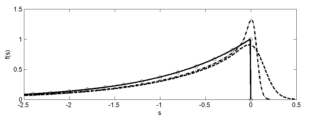
Figure 3: Quasi-equilibrium distributions for infrequently (4%) positive mutations (dashed line – double-exponential mutations; dash-dotted line – shifted exponential mutations) and equilibrium distributions for non-positive mutations (solid line – numerical simulations; circles – exponential distribution )

The mutations are non-positive when $b_{2}=\infty$ in (26) or $\zeta_{0}=0$ in (29). The mutations, however, become infrequently positive when $b_{2}$ is large or $\zeta_{0}$ is small. The exact analytical solution $f_{0}=\exp(y-y_{\ast})$ for non-positive mutations is shown in Figure 3 by the solid line. The other lines show the distribution $f(y,y_{\ast})$ for the process of competitive escalation with $4\%$ of positive mutations (i.e. $1/b_{2}=\zeta_{0}=0.04$). The simulations are performed with 1000000 Pope particles. Mutations (26) and (29) correspond to the dashed and dotted lines. The formula determining the rate of competitive escalation, which was derived in Ref. [5], can be written as

$$\frac{dy_{\ast}}{dt}=\frac{c_{0}}{\Delta t}\left\langle\zeta H(\zeta)\right\rangle\approx\frac{c_{0}}{\Delta t}\frac{\beta}{\hat{\beta}^{2}},$$ (30)

where $H$ is the Heaviside function, $\Delta t$ is the time step and $c_{0}$ is a constant depending on the distribution of mutations. The approximate evaluation of $dy_{\ast}/dt$ is performed in (30) for $b_{2}\gg b_{1}$ in the double-exponential distribution (26), indicating that the effective selection rate of the competition process is given by $d\hat{s}_{\ast}/dt\sim-\beta/\hat{\beta}.$ The constant is $c_{0}\approx 5.4$ for (26), $c_{0}\approx 3.2$ for (29) and $c_{0}\approx 3.7$ for the uniform distribution of mutations considered in Ref. [5].

6 Thermodynamics of intransitive competition.

Competition is intransitive if at least one intransitive triplet

$$\mathbf{y}_{p}\preccurlyeq\mathbf{y}_{q}\preccurlyeq\mathbf{y}_{r}\prec\mathbf{y}_{p}\$$ (31)

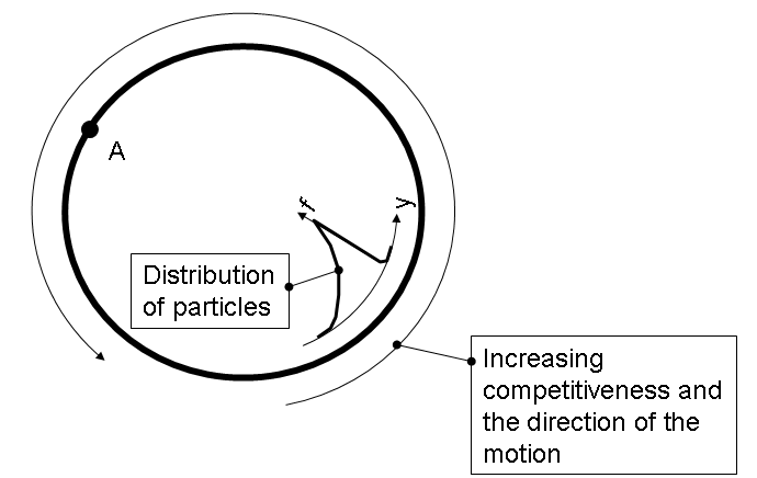
Figure 5: Current transitivity in completely intransitive competition.

exists in the system. Generally, a consistent absolute ranking can not be introduced for intransitive competition, but ranking can often be assigned to subdomains if the competition is transitive within these subdomains. It should be noted, however, that the rankings assigned in different subdomains would result in multi-valued functions and can not be made fully consistent with each other when the competition is intransitive (see the example in Figure 5). Relative rankings are valid for all competitive systems irrespective of their transitivity. The problem of introducing ranking in intransitive tournaments has been treated in a number of relatively recent publications [73, 74]. Our choice of ranking specified by (18)-(20) is based on consistency with the evolution induced by competitive mixing. The term “ordering” conventionally refers to transitive orders while intransitive binary relationships may be called “preferences” or “tournaments”. The term “tournament” seems to have become common in recent publications [75], unfortunately, this term is likely to be confusing in the context of the present work.

6.1 Intransitivity and its physical reasons

Although the fact that intransitivity may appear as the result of superimposing several perfectly transitive rules has been known since the days of French revolution as the Condorcet paradox (this paradox was noted first by outstanding mathematician, philosopher and humanist marquis de Condorcet [7]), intransitivities were viewed for a long time as something illogical or undesirable [76]. For example, if someone prefers A to B, B to C and C to A, can we see this individual as behaving reasonably? According to the famous Arrow theorem [77], the problem of intransitivity may pose a problem to choice in democratic elections. McGarvey[78] proved that any intransitive preferences on a finite set can be represented as a majority superposition of a finite number of transitive orders. Intransitivities have become more philosophically accepted in recent times [79] and are now commonly used in physics [80], biology [81] as well as in social and economic studies [73, 74, 75].

Conventional thermodynamics is fundamentally transitive and the thermodynamics of transitive competition is similar to conventional thermodynamics in this important respect. We cannot expect competitiveness to increase indefinitely, as it is likely to have some physical constraints even if an external source of exergy exempts the system from being isolated and subject to the immediate constraints of conventional thermodynamics. As shown in the previous section, if the leading element of the distribution reaches the point of maximal possible rank in transitive competition, any further development in the system is terminated. In conventional thermodynamics, this point is represented by the global equilibrium with maximal entropy or minimal Gibbs/Helmholtz free energy. The highly competitive group with maximal ranking would prevent any alternatives from a successful challenge; the system then stops evolving any further. One may hope that once a transitive equilibrium is reached, the creative hand of nature changes external conditions in a “right” direction so that the complex development may resume. Unless the complexity of this intervention is at least comparable with the complexity of the evolving systems, the long-term efficacy of such intervention seems doubtful. In most cases stable systems only slightly alter their states to attain a new equilibrium and compensate for the environmental disturbance. It seems that transitive description is an oversimplification of the complex (and often cyclic) behaviours observed in realistic competitive systems. Transitivity of competitive thermodynamics is not guaranteed a priori and depends on transitivity of the competition rules. Multiplicity of competitiveness criteria combined with a rather limited number of outcomes (i.e. winner or loser) is most likely to produce intransitivities due to the same reasons that were first discovered in the Condorcet paradox. Systems with intransitive competition rules must have an external source of exergy or negentropy [82], since isolated systems are subject to the constraints of conventional thermodynamics and must be transitive. Complex behaviour is known to occur far from equilibrium of conventional thermodynamics [1], since Onsager’s reciprocal relations do not allow for cycles and enforce transitivity close to the equilibrium.

6.2 Types of intransitivity

Any intransitive relation has its transitive closure — another relation that is transitive and is, as much as possible, close to the original relation (see Appendix A for details). We denote the transitive closure of our original competition rules by “$\prec_{t}$”, “$\succ_{t}$” and “$\simeq_{t}$”. It is useful to distinguish the following possibilities.

1. By transitive closure:

   1. Completely intransitive competition: all elements are transitively equivalent, i.e. $\mathbf{y}_{p}\simeq_{t}\mathbf{y}_{q}$ for any $p$ and $q.$ In terms of the original relation, any two elements $p$ and $q$ are a part of at least one intransitive loop

      $$\mathbf{y}_{p}\preccurlyeq\mathbf{y}_{1}\preccurlyeq\mathbf{y}_{2}...\preccurlyeq\mathbf{y}_{q}\preccurlyeq\mathbf{y}_{1}^{\prime}\preccurlyeq\mathbf{y}_{2}^{\prime}...\preccurlyeq\mathbf{y}_{p}$$ (32)

   2. Intransitive competition having a transitive component: the transitive closure involves several transitively unequal classes. In this case, $\mathbf{y}_{p}\succ_{t}\mathbf{y}_{q}$ requires $\mathbf{y}_{p}\succ\mathbf{y}_{q}.$

2. By localisation:

   1. Locally intransitive competition: intransitive triplets can be found in the vicinity of any point

   2. Intransitive competition with local transitivity: the domain of properties can be divided into subdomains so that the competition is transitive within each subdomain (but not in the whole domain)

If competition has a transitive component, an absolute ranking $r_{t}$ corresponding to this component can be introduced. This ranking, however, would be the same for all elements from the same transitive class, i.e. $r_{t}(\mathbf{y}_{p})=r_{t}(\mathbf{y}_{q})$ for $\mathbf{y}_{p}\simeq_{t}\mathbf{y}_{q}$ while it might be the case that $\mathbf{y}_{p}\succ\mathbf{y}_{q}$ or $\mathbf{y}_{p}\prec\mathbf{y}_{q}.$ If competition is locally transitive, rankings can be introduced for each transitive subdomain but can not be consistently extended to the whole domain. In general, a complex competition may involve a sophisticated hierarchy of transitive and intransitive rules. For example, intransitive competition may have a locally transitive component or intransitive competition may be locally transitive and have a transitive component, etc.

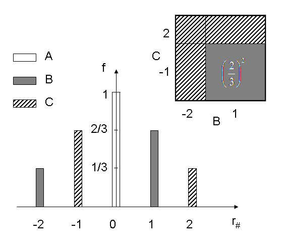
Figure 4: Competitive version of the Condorcet paradox: an example of intransitivity of group co-ranking $[f_{\mathop{\mathrm{A}}}]\prec[f_{\mathop{\mathrm{B}}}]\prec[f_{\mathop{\mathrm{C}}}]\prec[f_{\mathop{\mathrm{A}}}]$ occuring when the underlying competition is strictly transitive and determined by absolute ranking $r_{\#}$. Competition is presumed to be non-preferential. The square demonstrates that $[f_{\mathop{\mathrm{B}}}]\prec[f_{\mathop{\mathrm{C}}}]$ since B wins over C only in 4/9 of all cases.

Intransitivities may be also distinguished by their origin. A common source of intransitivity is superimposition of perfectly transitive rules. For example, comparison of subsystems by co-ranking (that is $[f_{\mathop{\mathrm{A}}}]\preccurlyeq[f_{\mathop{\mathrm{B}}}]$ when $\bar{R}([f_{\mathop{\mathrm{A}}}],[f_{\mathop{\mathrm{B}}}])\leq 0$) can exhibit intransitive properties even if the underlined competition between particles is strictly transitive. This can be interpreted as a variation of the Condorcet paradox[7]. The example of three distributions of particles $f_{\mathop{\mathrm{A}}}$, $f_{\mathop{\mathrm{B}}}$ and $f_{\mathop{\mathrm{C}}}$ such that $[f_{\mathop{\mathrm{A}}}]\prec[f_{\mathop{\mathrm{B}}}]\prec[f_{\mathop{\mathrm{C}}}]\prec[f_{\mathop{\mathrm{A}}}]$ is shown in Figure 4. We may interpret the sybsystems as competing super-elements but should expect that the rules for this competition are intransitive irrespective of the transitivity of the original competition rules.

6.3 Gibbs mutations in intransitive systems.

If mutations are restricted to Gibbs mutations, only one equilibrium distribution $f_{0}(\mathbf{y})$ is possible in the case of complete intransitivity since mutations defined by equation (54) propagate to the whole of the domain through the chain (32). Different equilibriums, however, are possible when the competition has a transitive component. Since the component ordering denoted by $\succ_{t}$ is transitive, an absolute ranking can be introduced so that $r_{t}(\mathbf{y}_{p})\leq r_{t}(\mathbf{y}_{q})$ is equivalent to $\mathbf{y}_{p}\preccurlyeq_{t}\mathbf{y}_{q}$. If intransitive competition has a transitive component, the system behaves with respect to this component as discussed in the previous section. The equilibrium distributions can be written as $f_{0}(\mathbf{y},r_{\ast})$ where $r_{\ast}$ is the ranking of the leading class and $r_{\ast}$ may increase if some positive mutations are present in the system. The H-theorem (Theorem 1) apply to Gibbs mutations irrespective of the transitivity of the competition.

6.4 Current or local transitivity

Distribution of a finite number of particles may be confined to a much smaller region (we can call it current region) as compared to the region of strict positiveness $f>0$ of the function $f(\mathbf{y})$: particles can not be found in the region where $f(\mathbf{y})$ is formally positive but very small. Competition in the current region may be transitive while remaining intransitive in larger regions. We can characterise this situation as currently transitive distribution. Currently transitive distributions behave over short period of time as if the competition is transitive. This case is illustrated in Figure 5. The competition shown in this figure is completely intransitive and an equilibrium distribution spreads over the whole domain. If the system is invariant with respect to shifts along the circle, this equilibrium distribution must be uniform. There is, however, another possibility when the number of particles is limited: the equilibrium distribution of particles can be confined to a narrow segment of the circle since $f$ in the rest of the domain is too small to be taken into account. If some rare positive mutations are present in the system, this distribution will keep cycling around the circle indefinitely. In this example, the competition is completely intransitive but currently transitive.

6.5 General mutations in intransitive systems.

In transitive competition, systems with general mutations behave in a qualitatively similar way as compared to systems with Gibbs mutations. This is not necessarily the case when competition is intransitive. In the absence of mutations, all non-trivial stationary distributions tend to produce oscillations (unless $R_{pq}=0$ for all non-isolated $p$ and $q$ — see Appendix D). Instabilities can also be expected in intransitive systems if the level of mutations is insufficient. Although there is a large diversity of possibilities in intransitive competitions, the behaviour of the systems may be predicted when certain restrictions apply. Intransitivity may be weak and dominated by transitive relations. If competition is intransitive but has a transitive component, the system would behave with respect to this component in a way that is similar to the case of general mutations in transitive systems. The ranking associated with the transitive component can stay constant or increase in time. A similar behaviour can be expected for competition that is currently transitive. The distribution evolves as if the competition is transitive over a short period of time but the system may appear to be cyclic over longer periods as illustrated in Figure 5. Absolute ranking can be introduced within a sector of the circles in Figure 5 but not over the whole domain. Cyclic behaviour is common for intransitive competition: at any given moment the system seems to progress forward but after the cycle is completed, it finds itself in the original state. Changes that seem to be improvements at a given time may prove to be detrimental in the long run.

Although intransitive competition does not guarantee a global improvement in competitiveness of a system, we still may expect some degree of local consistency with competitive thermodynamics. Since there is generally no absolute ranking in intransitive competition, we can use a relative ranking measured with respect to current distribution $f^{\circ}=f(\mathbf{y},t^{\circ})$ that is $r^{\circ}(\mathbf{y)}=r(\mathbf{y},[f^{\circ}])$ and $\bar{R}^{\circ}([f])=\bar{R}([f],[f^{\circ}])$. The distribution $f^{\circ}$ remains fixed and, as $f(\mathbf{y},t)$ evolves, $f$ becomes more and more different from $f^{\circ}$. We, however, consider a short-term development of $f,$ when $f$ stays close to $f^{\circ}.$ According to the evolution equation (78), the competition step $\delta f_{c}$ always improves current ranking $\bar{R}^{\circ}([\delta f_{c}])>0,$ but tends to decrease the configurational entropy $S_{c}$. The following mutation step $\delta f_{m}$ tend to decrease ranking $\bar{R}^{\circ}([\delta f_{m}])<0,$ since most of the mutations are non-positive and increase the configurational entropy $S_{c}$, since mutations are random. In a steady case $f=f_{0}$ all these changes compensate each other and entropy defined by equation (9) reaches its maximum. It is possible, however, to have a nearly steady state which is stable but continues to evolve slowly, that is $f_{0}=f_{0}(\mathbf{y,y}_{\ast}^{\circ})$ where $\mathbf{y}_{\ast}^{\circ}$ is the $f^{\circ}$-graded leading particle (the particle from the distribution $f$ with the maximal ranking $r_{\ast}^{\circ}=r(\mathbf{y}_{\ast}^{\circ},[f^{\circ}])$ ). In many cases $r_{\ast}^{\circ}=r_{\ast}^{\circ}(t)$ tends to increase in time and conditions sufficient to ensure this can be nominated (for example possessing a current transitivity or a transitive component). It seems, however, that cases of decreasing $r_{\ast}^{\circ}(t)$ are also possible in some circumstances: we call these cases competitive degradations. There are indications (Section 7.4) that degradations are accompanied by an increase in chaotic behaviour and it may be the case that properly defined overall entropy still increases, although there is no certainty. Competitive degradations, which are competition failures, should be distinguished from erosive degradations, which are induced by physical inabilities of the system to retain information as needed or by partial suppression of the competition.

The intransitive competition process is blind and can not guarantee long term absolute increase in rankings. Ranking in intransitive competition becomes relative: what seems to be a competitive improvement now may later appear to be a loss of competitiveness. It is natural, however, that competition improves the current relative ranking $\bar{R}^{\circ}([f])=\bar{R}([f],[f^{\circ}])$. The example shown in Figure 5 illustrates the case when the current ranking $\bar{R}^{\circ}([f])$ increases as the distribution $f(\mathbf{y,y}_{\ast}^{\circ}(t))$ moves counterclockwise. This distribution, however, may lose its stability and collapse due to disturbances located at point A, since ranking of the distribution with respect to point A decreases as $\mathbf{y}_{\ast}^{\circ}(t)$ gets closer to A. Hence, decline and collapse may be caused by both of the factors mentioned above: direct competitive degradations accompanied by reduction of $\bar{R}^{\circ}([f])$ and by short-term escalation of ranking $\bar{R}^{\circ}([f])$ that appears to be detrimental to the stability of the distribution over a long run.

7 Examples of different behaviours observed in competitive systems

Without implying that competitive behaviour must be limited to the modes listed below, we distinguish the following types of behaviour in realistic systems:

1. Stable equilibrium. A competitive system remains in this state indefinitely unless surrounding conditions are changed.

2. Competitive escalation. A competitive system reaches a quasi-equilibrium state and continues to slowly evolve in the direction of increasing competitiveness

3. Invasion wave is a rapid escalation occurring in a propagating wave. This process is inhomogeneous.

4. ^∗Regular cycle. Competitive escalation with respect to the current distribution results in recurrence of the same conditions due to cyclic intransitivity.

5. ^∗Competitive cooperation and self-organisation. Under certain conditions when competition is intransitive and localised in physical space, the elements tend to form cooperative structures (with a reduced level of competition within the structure) and collectively struggle for domination over other structures.

6. ^∗Competitive degradation. A system reaches a quasi-equilibrium state which slowly loses its competitiveness.

7. ^∗Leaping cycle. A structure quickly rises to dominance, holds a dominant position and then weakens due to competitive degradation or loss of stability and rapidly collapses. If the competition has a transitive component, each subsequent cycle should be somewhat different from the previous one, so that the evolution of the system resembles a spiral.

8. ^∗Unstable and/or stochastic behaviour. A system does not have a stable equilibrium (or quasi-equilibrium) and possibly evolves in an irregular manner.

The types of behaviour marked by the asterisk can be observed only in intransitive systems. An example of a stable equilibrium is given by non-negative mutations in transitive competition. Competitive escalation is related to positive mutations, whose effect is shown in Figure 3. Turbulent premixed flames give an example of invasion waves [6]. Competitive cooperation, self-organisation and competitive degradation have been detected to occur in intransitive systems with localisation of mixing in physical space [5]. While transitive behaviour is more consistent with conventional thermodynamics, which is constrained by its zeroth law and is fundamentally transitive, complex behaviour in competitive systems is associated with intransitivity. Examples of intransitive competitions are considered below.

7.1 Turbulent flows

Turbulence is a complex phenomenon which can provide examples of intransitive behaviour. One of the possible examples of turbulent intransitivities is illustrated in Figure 6, which shows the routes for kinetic energy exchange between different Reynolds stresses in a turbulent shear flow[13]. Energy is supplied from the mean shear and dissipated at the smallest scales. This supply/dissipation process, however, is not uniform: competition for energy between different Reynolds stresses occurs in an intransitive manner as shown in Figure 6. In general, the cyclic nature of the energy exchange shown in the figure may produce oscillations during rapid distortions but it seems that dissipation, which is strong in turbulent flows, tends to dampen these oscillations in most cases.

7.2 Belousov-Zhabotinsky reaction

Intransitivities are possible in chemical reactions. The Belousov-Zhabotinsky reaction is known to display a cyclic chemical behavior in a homogeneous mixture, which is unusual since most chemical kinetics tend to monotonically converge to an equilibrium or steady state. If the reactants denoted by A and B are supplied to the system and the product P is removed from the system, the oscillations of concentrations can continue indefinitely. The simplest chemical kinetic scheme that can adequately simulate the Belousov-Zhabotinsky reaction is Oregonator [83]. This scheme involves an essential intransitivity related to the following cycle X$\rightarrow$Z$\rightarrow$Y$\rightarrow$X$\rightarrow$…, schematically depicted in Figure 7. It should be noted that this cycle has to be powered by external sources of exergy (supply of reactant A and B in this case) since autonomous conversion of X into Z then into Y then into X is impossible due to transitive constraints of conventional thermodynamics.

Although the Oregonator system involves only three active elements X, Y and Z, its cycle deviates from a regular cycle and has some features of the leaping cycle: the phase of rapid expansion X$\rightarrow$Z$\rightarrow$Y is followed by a slow decay of Y until the system loses stability and a new pulse of injection of X repeats the cycle.

7.3 Oscillations in the scissors–paper–rock system

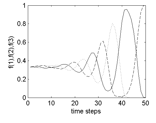
Figure 8: Regular cycle in intransitive competition without mutations

Consider a system that has three states: 1) paper, 2) scissors and 3) rock. The competition rules are intransitive and given by $1\prec 2\prec 3\prec 1$. No mutations are present in the system. The initial distribution is given by $f(1)=f(2)=f(3)=1/3$. This distribution is stationary due to the symmetry of the competition rules. According to Appendix D, oscillations are expected in this system, while finite time steps make these oscillations mildly unstable. Figure 8 demonstrates evolution of this system.

7.4 Intransitive competition and competitive cooperation

The figures presented below are obtained from computer simulations of abstract competition. In these simulations, particle properties are represented by the vector $\mathbf{y}=(y^{(1)},$ $y^{(2)},$ $y^{(3)})$, which satisfies the conservation constraint $y^{(1)}+y^{(2)}+y^{(3)}=1$ and is interpreted as a combination of the primary colors: red, green and blue. The competition is controlled by the Condorcet rules representing the majority superposition of the following orderings: $y_{p}^{(i)}<y_{q}^{(i)}$, $i=1,2,3$ for every given couple $p$ and $q$. These rules are locally intransitive and intransitive triplets $\mathbf{y}_{p}\mathbf{\prec y}_{q}\mathbf{\prec y}_{r}\mathbf{\prec y}_{p}$ can be found in a vicinity of any point $p$ in the property space. The competition process is localised in the physical space. The physical domain is 2-dimensional and is mapped into a rectangle in the images presented here. None of the primary colors has any competitive advantages over the other primary colors but particles may have different overall competition strength with brighter colors performing on average better than the darker colors. Particle colors change according to the competition rules and predominantly negative random mutations. Otherwise, there is no coordination of any kind over the particle properties. The competition rules and process parameters do not change during the simulations. The details of the methodology of these competitive simulations can be found in Ref.[5]. We stress that the complex behavior observed in these simulations is linked to intransitivity and localisation of the competition.

The formation of a spot-like structure, which is observed in intransitive simulations with localisation of competition effective volume in physical space, reduces the intensity of competition. This reduction can be interpreted as a competitive cooperation between the particles. The particles of a dominant color manage to dominate collectively while reducing their overall competition effort. The intensity of competition is the average magnitude of adjustments of the properties of the losers $\Xi=2\Sigma_{p}\left|\mathbf{\acute{y}}_{p}-\mathbf{y}_{p}\right|/n,$ where the sum is taken over $n/2$ losing particles. There are two major factors that reduce the competition intensity. The competition is, obviously, less intense within a spot filled with similar colors than between the spots having very different colors. Within a spot, particles of different competitive strengths tend to compete at their own level of strength.

The curves in Figure 9 represent the intensity of the primary colors $y^{(i)}$, $i=1$ (red), 2 (green) and 3 (blue) averaged over all particles and plotted versus the number of time steps. The simulations display leaping cycles: a color leaps into a dominant position of controlling the domain and manages to fend off competitors for a while, but ultimately reduces its competitiveness due to competitive degradation and loses competition to new challenges. The periods of clear dominance of a color are interchanged with periods of chaotic struggle without a clear winner or by periods of dominance of another color. The figure also presents configurations entropy $S_{c}$ determined for $A=1,$ ranking $\bar{R}_{u}([f])=\bar{R}([f],[f_{u}])$ relative to the uniform distribution $f_{u}=\mathop{\mathrm{c}onst}$ and the intensity of competition $\Xi$. It is clear that the loss of ranking $\bar{R}_{u}$ brings a more chaotic behaviour into the system – negative correlation between $S_{c}$ and  $\bar{R}_{u}$ is prominent. More chaotic behaviour tends to increase the intensity of competition $\Xi$. Figure 10 shows two consecutive states of the system (the property space on the left and the physical space on the right) when a newborn structure takes control over a chaotic behaviour and becomes highly dominant until it gradually weakens and loses its dominant position. Note the pyramid-like cooperative structures in the property space — within these structures the competition tends to be stratified and occur between particles with close properties and ranks.

8 Summary and conclusions

This work reviews existing publications and introduces a number of new results related to the application of non-conventional thermodynamics to turbulence, combustion and general non-equilibrium competitive processes involving different forms of mixing.

8.1 Competitive mixing.

The possibility of application of general principles of thermodynamics to competitive systems is reviewed and investigated. In its abstract form, competition is essentially a type of mixing, (i.e. competitive mixing), which can be effectively represented by a system of Pope particles and used to simulate a wide range of non-equilibrium processes including turbulent mixing and combustion. Although abstract competition should have a wide interdisciplinary range of applications, examples mentioned in this work are mainly restricted to turbulent flows, chemical reactions and combustion, which are the author’s prime areas of interest. In applications not related to turbulence, the concept of competitiveness represents a logical extension of the concepts of fitness and/or utility. Although abstract competition has been derived from a single field (turbulent combustion), it seems to represent an interdisciplinary approach linking distant fields and concepts (adiabatic accessibility and economic preferences may serve as an example).

8.2 Competitive thermodynamics.

Thermodynamic description of stochastic systems can be very useful and is repeatedly used in the literature but, in application to complex systems, thermodynamics does have its limitations discussed below. Entropy is the key quantity in thermodynamics, while the other thermodynamic properties are linked to the definition of entropy. During last decades it has become conventional to use the term entropy in different contexts, ranging from mathematics to social sciences. The same trend can be observed in studies of turbulent flows, where different physical quantities may be implied under this term. In the present work we use the term “apparent” to distinguish entropy-like quantities from molecular entropy.

We introduce a special type of random disturbances present in competition — the Gibbs mutations which possess certain Markov-like properties — and demonstrate that general principles of competition are consistent with thermodynamic description. Competitive entropy is subject to the competitive H-theorem presented in Appendix D. A competitive system can also be characterised by another thermodynamic quantity — the competitive potential, which determines the likely direction of evolution of the system. A competitive system can be generally expected to stay in equilibrium or gradually increase its competitive potential over time. Contested resources tend to move between systems from lower to higher values of the competitive potential. In premixed combustion, products have higher entropy than the reactants and thus are more competitive. In the same manner, more competitive species invading areas occupied by less competitive species should be assigned a higher value of the effective entropy. Competitive thermodynamics recognises the obvious trend of moving towards more competitive states, irrespective of the exact nature of this competitiveness. The adiabatic accessibility approach, the theory of Gibbs measures and the principles of non-equilibrium thermodynamics should be mentioned here as important results preceding competitive thermodynamics. The overall rate of selection is linked to the frequency of positive mutations, which is constrained by the fluctuation theorem and other thermodynamic parameters.

The analogy with conventional thermodynamics is established first for Gibbs mutations but, if competition is transitive, any system with weakly positive mutations of a general nature would behave in a qualitatively similar manner to Gibbs systems: the system would quickly reach its quasi-equilibrium and then slowly escalate towards more competitive states until the point of maximal competitiveness is reached. After this, no further evolution can occur in the system as long as the external conditions remain fixed. In principle, a transitive competitive system, which is decoupled from molecular thermodynamics by an external source of exergy, may escalate its competitiveness indefinitely but, practically, there should be some physical limits on how high this competitiveness could be. Any equilibrium represents a balance between the forces of chaos and the forces of order. Thus, from the perspective of competitive thermodynamics, some degree of order appearing out of chaos in competitive systems should be expected in the same way as more ordered crystalline states can appear in conventional thermodynamics under appropriate conditions. From the perspective of competitive thermodynamics, order appearing in some conventionally non-equilibrium competitive processes is, by itself, no more or less surprising than the possible presence of order in equilibrium states of conventional thermodynamics.

8.3 Intransitivity.

The main argument presented in this paper is, however, not about similarities of conventional and competitive thermodynamics, but about their differences. In the case of relatively simple systems, transitive competition and transitive thermodynamics produce a plausible picture of monotonic motion towards competitive equilibrium. This, however, does not seem to be consistent with the endlessly vigorous and often cyclic behaviour observed in complex competitive systems. However, if the competition rules are allowed to be intransitive, new types of complex behaviours emerge within the systems. The elements may form structures with a reduced level of competition within the structure (i.e. competitive cooperation) and struggle collectively to dominate the allowable space. Endless cyclic behaviour seems to become quite common under intransitive conditions: cooperative structures tend to survive and dominate for some time only to degrade at the end and be replaced by new structures. Intransitive systems can not be thermodynamically isolated, as this would immediately impose the transitive constrains of conventional thermodynamics, but require a relatively simple form of intervention — an external source of exergy. The choice in favour of considering intransitivities needs to be made not because intransitivity can immediately explain all the complexities of the surrounding world but because transitive competition certainly cannot. This does not prevent many specific features from having perfectly transitive explanations, while intransitivity is associated with more complex effects.

The early success of classical thermodynamics was associated with recognition of the irreversibility of the world around us, in spite of the time reversibility adopted by classical physics. It is difficult to make a general statement but abstract competition seems to point towards intransitivity, and the number of publications dedicated to different aspects of intransitivity is on the rise. We thus might have to face another difficult task of recognising the intransitivity of the surrounding world in contrast with the natural preference for the simplicity of the transitive description. In the transitive world, we have clear signposts: “strong” versus “weak”, “fit” versus “unfit” and so on. The intransitive word is much more relativistic: a strategy that seems to be a big winner today may prove to be disastrous in a long run. We do not like intransitivities, not because they do not exist, but because they cause complications and it is generally difficult to treat them in a logical manner. This, however, is exactly the reason why intransitivities should be studied — they are responsible for the complexity of the world around us. The reasons behind the ubiquitousness of intransitivity seem to be quite transparent and very much similar to the reasons behind the Condorcet paradox: intransitivity is common when the simple outcome “is” or “is not” depends on many factors and criteria. A complex system is characterised by a multiplicity of rules; even if each rule is perfectly transitive, it is quite likely that a superposition of these rules is not. An element of a system may represent a system on its own (i.e. subsystem) while co-ranking of subsystems is inherently intransitive (see the example shown in Figure 4). Another cause of intransitivity is that transitively weak elements tend to be removed by competition and further competition occurs in a more refined domain, where elements have similar ranks and intransitivities are likely.

8.4 Unresolved problems.

The theorems given in the Appendices establish major principles for evolution of competitive systems. It is worthwhile, however, to draw the attention of the reader to the immediate unresolved problems associated with intransitive behaviour. While competitive thermodynamics is useful when competition is intransitive but retains some transitive properties (such as being currently transitive or having a transitive component) or when mutations are not much different from Gibbs mutations, the feasibility of thermodynamic treatment of general mutations combined with general intransitivity is under the question mark. The analogy with conventional thermodynamics works well for simpler competitions but it seems to become less suitable for complex cases.

Competitive degradations are an outcome of competition that seems abnormal from the perspective of apparent thermodynamics, but they appear to be possible in intransitive competitions. It seems that competitive cooperation, which also becomes possible in intransitive systems and is one of the key signs of complex behaviour, has a penalty of competitive degradation attached to the benefits of competitive cooperation. Establishing necessary and sufficient conditions for the existence of competitive degradations is an outstanding problem.

8.5 Conclusion

Competitive thermodynamics, whose concept has been derived from the modelling of turbulent combustion by competitive mixing, indicates that transitive evolution of competitive systems is generally consistent with conventional thermodynamic principles. Studies of complex behaviour in competitive systems, however, need to move beyond the principles of conventional thermodynamics in order to take into account intransitivity, which is commonly present in nature and seems to be responsible for complex cooperative behaviour.

9 Acknowledgments

The author thanks D.N.P. Murthy for numerous discussions and S.B.Pope for insightful comments and suggestions. Suggestions made by the anonymous reviewers are also appreciated. The author thanks D.N. Saulov and D.A. Klimenko for useful comments and assistance in preparation of the manuscript. The wide scope of possible applications of this work is likely to make some omissions inevitable; any omissions, irrespective of their fields of application, are regretted by the author. The part of this work related to particle methods is supported by the Australian Research Council.

APPENDICES

Appendix A Transitivity and absolute ranking

This section gives a brief explanation of the mathematical terms and statements referred to in the main text.

A.1 Absolute ranking and Debreu theorem

Consider totally and transitively pre-ordered sets in Euclidean space or in a complete separable metric space:

• Totality implies that any two elements $p$ and $q$ are comparable, that is either $\mathbf{y}_{p}\preccurlyeq\mathbf{y}_{q}$ or $\mathbf{y}_{p}\succcurlyeq\mathbf{y}_{q}$ or both of these relations are correct and $\mathbf{y}_{p}\simeq\mathbf{y}_{q}$.

• Pre-ordering, unlike ordering, allows for $\mathbf{y}_{p}\simeq\mathbf{y}_{q}$ when $\mathbf{y}_{p}$ and $\mathbf{y}_{q}$ are not the same.

• Transitivity is defined as the following property: $\mathbf{y}_{p}\preccurlyeq\mathbf{y}_{q}$ and $\mathbf{y}_{q}\preccurlyeq\mathbf{y}_{r}$ always demands that $\mathbf{y}_{p}\preccurlyeq\mathbf{y}_{r}$ for any $p,$ $q$ and $r$.

• Continuity. Pre-ordering is continuous when the subsets $\mathfrak{D}_{\preccurlyeq}(\mathbf{y}^{\circ})=\{\mathbf{y}\;|\;\mathbf{y}\preccurlyeq\mathbf{y}^{\circ}\}$ and $\mathfrak{D}_{\succcurlyeq}(\mathbf{y}^{\circ})=\{\mathbf{y}\;|\;\mathbf{y}\succcurlyeq\mathbf{y}^{\circ}\}$ are closed for any $\mathbf{y}^{\circ};$ or equivalently when for any converging sequence $\mathbf{y}_{p},$ $p=1,2,...$ selected from the set, the boundedness of the sequence by $\mathbf{y}_{p}\preccurlyeq\mathbf{y}^{\circ}$ (or $\mathbf{y}_{p}\succcurlyeq\mathbf{y}^{\circ}$) demands the corresponding boundedness of the limit $\mathbf{y}_{p}\rightarrow\mathbf{y}_{0}$ as$\;p\rightarrow\infty$ by $\mathbf{y}_{0}\preccurlyeq\mathbf{y}^{\circ}$ (or $\mathbf{y}_{0}\succcurlyeq\mathbf{y}^{\circ}$) for any $\mathbf{y}^{\circ}$. Physically, continuity of the ordering indicates a connection between ordering and the intrinsic metric of the space.

• Absolute ranking, which is a scalar function $r_{\#}(\mathbf{y)}$ defined on the set, is equivalent to pre-ordering when $r_{\#}(\mathbf{y}_{p}\mathbf{)\leq}r_{\#}(\mathbf{y}_{q}\mathbf{)}$ is equivalent to $\mathbf{y}_{p}\preccurlyeq\mathbf{y}_{q}$ for any $p$ and $q.$ Ranking is called continuous when the function $r_{\#}(\mathbf{y)}$ is continuous.

• Debreu theorem. The introduction of absolute ranking is subject to the Debreu theorem [69, 84] which states that equivalent absolute ranking $r_{\#}(\mathbf{y}_{p}\mathbf{)}$ can be introduced for any transitive total pre-ordering provided the pre-ordering is continuous. The ranking can be selected to be continuous.

Demonstrating the necessity of the continuity restriction imposed on pre-ordering is relatively easy. If the converging sequence $\mathbf{y}_{p}\rightarrow\mathbf{y}_{0}$ as$\;p\rightarrow\infty$ is bounded by $\mathbf{y}_{p}\preccurlyeq\mathbf{y}^{\circ}$ then the equivalent continuous ranks $r_{p}=r_{\#}(\mathbf{y}_{p})$ are bounded by $r_{p}\leq r^{\circ}=r_{\#}(\mathbf{y}^{\circ})$. The ranks $r_{p}$ converge to $r_{p}\rightarrow r_{0}=r_{\#}(\mathbf{y}_{0})$ since the ranking function is continuous. It is clear that $r_{0}\leq r^{\circ},$ otherwise convergence of the ranks to $r_{0}$ is impossible. Hence, we conclude that $\mathbf{y}_{0}\preccurlyeq\mathbf{y}^{\circ}$. The necessity of transitivity is also obvious. Indeed, let $\mathbf{y}_{p}\prec\mathbf{y}_{q}\prec\mathbf{y}_{r}\prec\mathbf{y}_{p}$ be an intransitive triplet. For equivalent ranking we then have $r_{\#}(\mathbf{y}_{p})<r_{\#}(\mathbf{y}_{q})<r_{\#}(\mathbf{y}_{r})<r_{\#}(\mathbf{y}_{p})$ and ranking in intransitive competition, if it exists, becomes a multivalued function.

The sufficiency part of the theorem, which is much more difficult to establish, has been proved by Debreu [69, 84] for topological second-separable spaces. The results of Lieb and Yngvason [3], who also postulated transitivity and continuity (although called the latter “stability”) for pre-ordering by adiabatic accessibility that, are consistent with the Debreu theorem.

The following examples illustrate the possibility or impossibility of absolute ranking:

• Lexicographic ordering. The example of a transitive preordering that is not continuous and can not have an equivalent ranking has been given by Debreu [69]. Consider lexicographic ordering of the plane $\mathbf{y}=(y^{(1)},y^{(2)})$. Let $\mathbf{y}_{p}\preccurlyeq\mathbf{y}_{q}$ when, by definition, either $y_{p}^{(1)}<y_{q}^{(1)}$ or $y_{p}^{(1)}=y_{q}^{(1)}$ and $y_{p}^{(2)}\leq y_{q}^{(2)}$ implying that $\mathbf{y}_{p}=\mathbf{y}_{q}$ when $y_{p}^{(1)}=y_{q}^{(1)}$ and $y_{p}^{(2)}=y_{q}^{(2)}$. The subsets $\mathfrak{S}(y^{(1)})=\{(y^{(1)},-\infty<y^{(2)}<+\infty)\}$ should have non-overlapping intervals of ranks $r_{\#}(\mathfrak{S}(y_{1}))\cap r_{\#}(\mathfrak{S}(y_{2}))=\emptyset$ when $y_{1}\neq y_{2}$. Since there is a non-countable number of subsets $\mathfrak{S}(y)$ and only a countable number of the intervals $r_{\#}(\mathfrak{S}(y_{1}))$, equivalent ranking is impossible.

• Countable sets. Equivalent ranking can always be introduced for any totally and transitively pre-ordered countable set. Let $\mathbf{y}_{1},\mathbf{y}_{2},...$ be the counting sequence that, of course, is generally not coincident with the ordering sequence. The first element $\mathbf{y}_{1}$ can be assigned any rank, say $r_{\#}(\mathbf{y}_{1})=0$. Assuming that equivalent ranks have been assigned to first $k$ elements from the counting sequence, we can always select a rank, which is consistent with the previous $k$ assignments, for the element numbered $k+1$. Repeating this procedure for the rest of the counting sequence assigns equivalent ranks to all elements.

• Measure-based ranking. If a measure $\mu$ is defined for the space under consideration, a relatively simple absolute ranking can be introduced for total transitive pre-ordering by

  $$r_{\mu}(\mathbf{y}^{\circ})=\mu\left(\{\mathbf{y\;}|\;\mathbf{y}\preccurlyeq\mathbf{y}^{\circ}\}\right)$$ (33)

  From a practical perspective, the measure-based ranking may be sufficiently accurate but, generally, it does not represent an equivalent ranking and may coarsen the original pre-ordering:

  1. if $\mathbf{y}_{p}\simeq\mathbf{y}_{p}$ then $r_{\mu}(\mathbf{y}_{p})=r_{\mu}(\mathbf{y}_{p})$

  2. if $r_{\mu}(\mathbf{y}_{p})<r_{\mu}(\mathbf{y}_{q})$ then $\mathbf{y}_{p}\prec\mathbf{y}_{q}$

  3. if $r_{\mu}(\mathbf{y}_{p})=r_{\mu}(\mathbf{y}_{q})$ then $\mathbf{y}_{p}\prec\mathbf{y}_{q}$ or $\mathbf{y}_{p}\succ\mathbf{y}_{q}$ or $\mathbf{y}_{p}\simeq\mathbf{y}_{q}$

A.2 Transitive closure

This subsection gives a brief explanation of transitive closures, which are commonly used in the analysis of intransitive relations; for more details see other publications, [75] for example. The transitive closure defines a new transitive relation “$\preccurlyeq_{t}$” that is consistent as much as possible with a given intransitive relation “$\preccurlyeq$”. Transitive closure is minimal i.e. additional relations, which are not needed to establish transitivity of existing relations, are not included in the closure. If “$\preccurlyeq$” is transitive than “$\preccurlyeq_{t}$” coincides with “$\preccurlyeq$”.

The closure involves several steps. For the sake of simplicity, we may presume that all elements are comparable so that elements in every pair are related by “$\prec$”, “$\succ$” or “$\simeq$”. These relations are first expressed in terms of “$\preccurlyeq$”, for example “$\prec$” means “$\preccurlyeq$” but not “$\succcurlyeq$”. Second, $\mathbf{y}_{p}\preccurlyeq_{t}\mathbf{y}_{q}$ is defined for any $p$ and $q$ that $\mathbf{y}_{p}\preccurlyeq\mathbf{y}_{q}$. Third, the new relation is transitively extended to new elements: whenever $\mathbf{y}_{p}\preccurlyeq_{t}\mathbf{y}_{q}\preccurlyeq_{t}\mathbf{y}_{r}$ it is also set that$\ \mathbf{y}_{p}\preccurlyeq_{t}\mathbf{y}_{r}$. The third step is repeated as long as necessary until these extensions do not introduce any new relations. Finally, $\mathbf{y}_{p}\simeq_{t}\mathbf{y}_{q}$ is defined when $\mathbf{y}_{p}\preccurlyeq_{t}\mathbf{y}_{q}$ and $\mathbf{y}_{p}\succcurlyeq_{t}\mathbf{y}_{q}$ (that is $\mathbf{y}_{q}\preccurlyeq_{t}\mathbf{y}_{p}$); while $\mathbf{y}_{p}\prec_{t}\mathbf{y}_{q}$ is defined when $\mathbf{y}_{p}\preccurlyeq_{t}\mathbf{y}_{q}$ but not $\mathbf{y}_{p}\succcurlyeq_{t}\mathbf{y}_{q}.$ The defined closure is transitive by definition.

The transitive closure divides all elements into one or more classes of equivalence $\mathfrak{C}_{I}$ where $\mathbf{y}_{p}\simeq_{t}\mathbf{y}_{q}$ when and only when $p$ and $q$ belong to the same class $I$. The classes are totally ordered by “$\prec_{t}$” so that $\mathbf{y}_{p(I)}\prec_{t}\mathbf{y}_{q(J)}$when and only when $\mathfrak{C}_{I}\prec_{t}\mathfrak{C}_{J},$ where $p(I)$ denotes any $p$ that belongs to class $I$. The transitive and intransitive relations are related to each other by:

• Within each class any two elements $p$ and $q$ are part of at least one loop with a changing but finite number of elements

  $$\mathbf{y}_{p}\preccurlyeq\mathbf{y}_{1}\preccurlyeq\mathbf{y}_{2}\preccurlyeq...\preccurlyeq\mathbf{y}_{q}\preccurlyeq\mathbf{y}_{1}^{\prime}\preccurlyeq\mathbf{y}_{2}^{\prime}\preccurlyeq...\preccurlyeq\mathbf{y}_{p}$$ (34)

  where all elements belong to the same class $\mathbf{y}_{p}\simeq_{t}\mathbf{y}_{1}\simeq_{t}...\simeq_{t}\mathbf{y}_{q}\simeq_{t}\mathbf{y}_{1}^{\prime}\simeq_{t}...\simeq_{t}\mathbf{y}_{p}$. The shortest possible loop has only two elements $\mathbf{y}_{p}\simeq\mathbf{y}_{p}$.

• The transitive relation coarsens the original relation , that is for any $p$ and $q$

  1. if $\mathbf{y}_{p}\simeq\mathbf{y}_{p}$ then $\mathbf{y}_{p}\simeq_{t}\mathbf{y}_{p}$

  2. if $\mathbf{y}_{p}\prec_{t}\mathbf{y}_{q}$ then $\mathbf{y}_{p}\prec\mathbf{y}_{q}$

  3. if $\mathbf{y}_{p}\simeq_{t}\mathbf{y}_{q}$ then $\mathbf{y}_{p}\prec\mathbf{y}_{q}$ or $\mathbf{y}_{p}\succ\mathbf{y}_{q}$ or $\mathbf{y}_{p}\simeq\mathbf{y}_{q}$

Appendix B Relative ranking in preferential competitions

This section gives a more general definition of ranking suitable for preferential mixing. These rankings are weighted by the preference function $\Psi_{pq}=\Psi(\mathbf{y}_{p},\mathbf{y}_{q}),$ which determines the probability of selecting the couple $p,q$ for mixing. This function is presumed bounded $0\leq\Psi(\mathbf{y}_{p},\mathbf{y}_{q})\leq 1.$ If mixing is non-preferential $\Psi=1$ for all particles; if particles $p$ and $q$ are isolated and can not mix $\mathbf{y}_{p}\parallel\mathbf{y}_{q}$ then $\Psi_{pq}=0$.

B.1 Losing and winning capacities

Relative ranking is related to losing and winning capacities. The generalised Heaviside step function

$$H(\mathbf{y},\mathbf{y}^{\prime})=\frac{R(\mathbf{y},\mathbf{y}^{\prime})+1}{2}=\left\{\begin{array}[]{c}0,\;\;\mathbf{y}\prec\mathbf{y}^{\prime}\\ \frac{1}{2},\;\;\mathbf{y}\simeq\mathbf{y}^{\prime}\\ 1,\;\;\mathbf{y}\succ\mathbf{y}^{\prime}\end{array}\right.$$ (35)

has the following properties

$$H(\mathbf{y},\mathbf{y}^{\prime})=1-H(\mathbf{y}^{\prime},\mathbf{y})$$ (36)

$$R(\mathbf{y},\mathbf{y}^{\prime})=H(\mathbf{y},\mathbf{y}^{\prime})-H(\mathbf{y}^{\prime},\mathbf{y}),$$ (37)

We denote $H_{pq}=H(\mathbf{y}_{p},\mathbf{y}_{q})$ and define winning and losing capacities of a particle by relationships

$$h^{+}(\mathbf{y}_{p}\mathbf{,[}f])=\underset{\infty}{\int}\Psi(\mathbf{y}_{p},\mathbf{y}_{q})H(\mathbf{y}_{p},\mathbf{y}_{q})f(\mathbf{y}_{q})d\mathbf{y}_{q}=\frac{1}{n}\sum_{q}\Psi_{pq}H_{pq}$$ (38)

$$h^{-}(\mathbf{y}_{p}\mathbf{,[}f])=\underset{\infty}{\int}\Psi(\mathbf{y}_{p},\mathbf{y}_{q})H(\mathbf{y}_{q},\mathbf{y}_{p})f(\mathbf{y}_{q})d\mathbf{y}_{q}=\frac{1}{n}\sum_{q}\Psi_{pq}H_{qp}$$ (39)

Here, as an example, we give both the continuous and discrete forms, assuming that the distribution $f(\mathbf{y}_{q})$ is represented by a large number of particles $q=1,...,n$. The average winning capacity of one distribution $f_{1}(\mathbf{y})$ with respect to another $f_{2}(\mathbf{y})$

$$\bar{H}([f_{1}],[f_{2}])=\underset{\infty}{\int\int}\Psi(\mathbf{y}_{1},\mathbf{y}_{2})H(\mathbf{y}_{1},\mathbf{y}_{2})f_{1}(\mathbf{y}_{1})f_{2}(\mathbf{y}_{2})d\mathbf{y}_{1}d\mathbf{y}_{2}$$ (40)

represents an average of $h^{+}(\mathbf{y}_{1}\mathbf{,[}f_{2}])$ where $\mathbf{y}_{1}$ is distributed with $f_{1}(\mathbf{y}_{1})$ and $\mathbf{y}_{2}$ is distributed with $f_{2}(\mathbf{y}_{2}),$ while $p_{1}=1,...,n_{1}$ and $p_{2}=1,...,n_{2}$ run over particle groups representing distributions $f_{1}$ and $f_{2}$ correspondingly.

B.2 Relative ranking and co-ranking

The effective relative ranking of a particle is then given by

$$r(\mathbf{y}_{p}\mathbf{,[}f])=\frac{h^{+}-h^{-}}{h^{+}+h^{-}}=\frac{\theta(\mathbf{y}_{p}\mathbf{,[}f])}{\psi(\mathbf{y}_{p}\mathbf{,[}f])}$$ (41)

where

$$\theta=h^{+}-h^{-}\;\mathop{\mathrm{a}nd}\;\psi=h^{+}+h^{-}$$

is the connectivity of particle $p$ to distribution $f(\mathbf{y})$: that is $\psi=1$ if mixing is non-preferential and $\psi=0$ if the particle is isolated from the distribution $f(\mathbf{y})$ which can be expressed by $\mathbf{y}_{p}\parallel[f]$. Relative $\Psi$-weighted ranking $r$ indicates the strength of particle $\mathbf{y}_{p}$ in competition with distribution $f(\mathbf{y})$ and $r_{p}=r(\mathbf{y}_{p}\mathbf{,[}f])$ may not be defined when $\mathbf{y}_{p}\parallel[f]$.

The relative ranking (co-ranking) of two distributions $f_{1}(\mathbf{y})$ and $f_{2}(\mathbf{y})$ is defined as

$$\bar{R}([f_{1}],[f_{2}])=\frac{\bar{\Theta}([f_{1}],[f_{2}])}{\bar{\Psi}([f_{1}],[f_{2}])}$$ (42)

where

$$\bar{\Theta}([f_{1}],[f_{2}])=\bar{H}([f_{1}],[f_{2}])-\bar{H}([f_{2}],[f_{1}])$$ (43)

and

$$\bar{\Psi}([f_{1}],[f_{2}])=\bar{H}([f_{1}],[f_{2}])+\bar{H}([f_{2}],[f_{1}])$$ (44)

is mixing connectivity of these two distributions. If $\bar{\Psi}([f_{1}],[f_{2}])=0,$ distributions $f_{1}(\mathbf{y})$ and $f_{2}(\mathbf{y})$ are isolated $[f_{1}]\parallel[f_{2}]$ and particles from these distributions do not compete with each other. The equations given above generalise equations (19) – (20) for preferential mixing.

B.3 Subsystem ranking

If the distribution $f(\mathbf{y})$ is divided into groups or subsystems $I=1,...,K$ so that

$$f(\mathbf{y})=\sum_{I=1}^{K}a_{I}\phi_{I}(\mathbf{y})$$ (45)

where the distributions $\phi_{I}(\mathbf{y})$ and constants $a_{I}$ are normalised, i.e.

$$\int_{\mathfrak{D}_{I}}\phi_{I}(\mathbf{y})d\mathbf{y}=1,\;\;\;\sum_{I=1}^{K}a_{I}=1$$

Each group of particles is generally presumed to be a subsystem, which is confined to a certain domain $\mathfrak{D}_{I}$ distinctive for each subsystem. The ranking of subsystems can be introduced as

$$\bar{R}_{I}=\bar{R}([\phi_{I}],[f])=\frac{\bar{\Theta}_{I}}{\bar{\Psi}_{I}}=\frac{1}{\bar{\Psi}_{I}}\sum_{J}a_{J}\bar{\Psi}_{IJ}\bar{R}_{IJ}$$ (46)

$$\bar{\Theta}_{I}=\bar{\Theta}([\phi_{I}],[f])=\sum_{J}a_{J}\bar{\Theta}_{IJ}$$ (47)

$$\bar{\Psi}_{I}=\bar{\Psi}([\phi_{I}],[f])=\sum_{J}a_{J}\bar{\Psi}_{IJ}$$ (48)

where $R_{IJ}$ represents the group co-ranking matrix

$$-\bar{R}_{JI}=\bar{R}_{IJ}=\bar{R}([\phi_{I}],[\phi_{J}])=\frac{\bar{\Theta}_{IJ}}{\bar{\Psi}_{IJ}}=\frac{\bar{\Theta}([\phi_{I}],[\phi_{J}])}{\bar{\Psi}([\phi_{I}],[\phi_{J}])}$$ (49)

If the subsystems $I$ and $J$ are isolated $[\phi_{I}]\parallel[\phi_{J}]$ then $\bar{\Psi}_{IJ}=0$ and co-ranking of these subsystems $R_{JI}$ is not defined. The possibility of treating the subsystems as new competing super-elements should be mentioned. Complex systems can be expected to have a hierarchy of subdivisions.

Appendix C Mutations

This section introduces Gibbs mutations that have some links with to Markov properties and Gibbs measures. Gibbs mutations are non-negative while near-Gibbs mutations can be infrequently positive. The distribution of infrequent positive mutations is analysed using thermodynamic considerations and the fluctuation theorem.

C.1 Gibbs mutations

The case of non-preferential mixing, where connections between Gibbs mutations, Markovian properties and Gibbs measures are most transparent, is considered first. A more general definition of Gibbs mutations for preferential mixing is given at the end of this subsection.

Let $f_{\zeta}(y,y^{\circ}\mathbf{)}$ be the probability distribution of mutations $y=y^{\circ}+\zeta$ originating at state $y^{\circ}$. Mutations we consider in this section are non-positive (i.e. $y^{\circ}+\zeta\preccurlyeq y^{\circ}$) and $f_{\zeta}$ is presumed to be free of singular components. The function

$$F_{\zeta}(y,y^{\circ})=\int_{-\infty}^{y}f_{\zeta}(y^{\prime},y^{\circ}\mathbf{)}dy^{\prime}$$ (50)

specifies the probability that ranking falls down to $r_{\#}(y)$ or below for mutations originating at $y^{\circ}$. Note that $F_{\zeta}(y,y^{\circ})=1$ for $y\succcurlyeq y^{\circ}$ since no positive mutations are allowed. In addition, the distributions of Gibbs mutations are required to satisfy the probability decomposition

$$F_{\zeta}(y,y^{\circ})=F_{\zeta}(y,y^{\prime})F_{\zeta}(y^{\prime},y^{\circ})$$ (51)

for any $y\preccurlyeq y^{\prime}\preccurlyeq y^{\circ}$. This condition can be interpreted as a Markov property. Indeed, consider mutations which occur continuously instead of a single jump and the motion down the ranks is terminated at a random moment. The Markov property requires that the termination moment depends only on the current location (and not on the state of origin of the mutation). With this property, equation (51) become almost obvious: in order to reach the state $y$ from $y^{\circ}$, a mutation needs to reach first the intermediate state $y^{\prime}$ and then proceed further to $y$. Differentiation of (51) with respect to $y$ yields

$$f_{\zeta}(y,y^{\prime})=\frac{f_{\zeta}(y,y^{\circ})}{F_{\zeta}(y^{\prime},y^{\circ})}$$ (52)

Another useful interpretation is treating each mutation as a sequence $y_{0},y_{1},...,y_{k}$ of a large number $k$ of small and stochastically independent steps $\Delta y_{i}=y_{i-1}-y_{i},$ $i=1,...,k$ so that $y_{0}=y^{\circ}$ is the mutation origin and $y_{k}=y$ is its final state. Each step $\Delta y_{i}$ is associated with effective energy $u_{i}$ so that step $i$ occurs with probability $\lambda_{i}=\exp(-u_{i})$ when and if the previous step $i-1$ is completed. If the step $i-1$ does not occur, then $u_{i}$ is taken to be infinite and the probability of step $i$ is zero. Hence the probability of reaching $y_{k}$ and beyond is given by the exponent

$$F_{\zeta}(y_{k},y_{0})=\prod_{i=1}^{k}F_{\zeta}(y_{i},y_{i-1})=\exp(-\sum_{i=1}^{k}u_{i})$$ (53)

which can be interpreted as a Gibbs measure [2]. This demonstrates the existence of a link between Gibbs mutations and Gibbs measures. Note the functional consistency of the equations (22), (51) and (52) and (53). As Gibbs measures, Gibbs mutations can be introduced on mathematical trees but we can approach more complex cases with a more general (but perhaps less physically transparent) definition.

Preferential mixing and mutations in more complex geometries need a more general approach to Gibbs mutations. The general definition of Gibbs mutations is given by the following expression for $f_{\zeta}(\mathbf{y},\mathbf{y}^{\circ})$

$$f_{\zeta}(\mathbf{y},\mathbf{y}^{\circ})=\frac{f_{0}(\mathbf{y})\Psi(\mathbf{y},\mathbf{y}^{\circ})}{h_{0}^{+}(\mathbf{y}^{\circ})}H(\mathbf{y}^{\circ},\mathbf{y})$$ (54)

where $h_{0}^{+}(\mathbf{y}^{\circ})=h^{+}(\mathbf{y}^{\circ},[f_{0}])$ is introduced. These mutations are non-positive ($\mathbf{y}+\mathbf{\zeta\;}\preccurlyeq\mathbf{y}$). Equation (22) can be easily recovered from (54) under simplifying assumptions. The H-theorem given in Appendix D demonstrates that the function $f_{0}$ in (22) and in (54) is, in fact, the equilibrium distribution specified by (7).

C.2 Fluctuation theorem

Consider an isolated thermodynamic system, which is characterised by the entropy $\hat{s}(y)$ and by corresponding equilibrium distribution

$$\hat{f}(y)\sim\exp\left(\hat{s}(y)\right)$$ (55)

The system changes its states though a random walk between the states $...,y_{-1},y_{0},y_{1},...$ by moving from the current node $i$ to its neighbour $i-1$ or $i+1$ with probabilities $\ \alpha_{i}^{-}$ and $\alpha_{i}^{+}$ correspondingly. The detailed balance at equilibrium requires that

$$\hat{f}_{i}\alpha_{i}^{+}=\hat{f}_{i+1}\alpha_{i-1}^{-},\;\;\hat{f}_{i}\sim\exp\left(\hat{s}_{i}\right)$$ (56)

where $\hat{f}_{i}$ is the discrete version of the equilibrium distribution and $\hat{s}_{i}=\hat{s}(y_{i})$. The condition (56) then takes the form

$$\frac{\alpha_{i}^{+}}{\alpha_{i+1}^{-}}=\frac{\hat{f}_{i+1}}{\hat{f}_{i}}=\exp\left(\Delta\hat{s}_{i}\right),\;\;\Delta\hat{s}_{i}=\hat{s}_{i+1}-\hat{s}_{i}$$ (57)

Let $\mathbb{P}(j^{\circ}\rightarrow j,k)$ be the probability of transition from node $j^{\circ}$ to node $j$ after exactly $k$ steps (assuming of course that $\left|j-j^{\circ}\right|\leq k$). Each given sequence $j^{\circ}\rightarrow...\rightarrow j$ can be reversed $j\rightarrow...\rightarrow j^{\circ}$ and we may assume $j\geq j^{\circ}$ without loss of generality. The ratio of probabilities of these direct and reverse sequences is now evaluated. The direct sequence has $j-j^{\circ}$ increasing steps ($i\rightarrow i+1$) and, possibly, a certain number of closed loops (i.e. subsequences that start and finish at the same location) while the reverse sequence has the $j-j^{\circ}$ of similar but decreasing steps ($i+1\rightarrow i$) and the exactly same number of the exactly same close loops as in the direct sequence. The ratio of probabilities becomes

$$\frac{\mathbb{P}\left(j^{\circ}\rightarrow j,k\right)}{\mathbb{P}\left(j\rightarrow j^{\circ},k\right)}=\frac{\mathbb{P}_{\Sigma 0}}{\mathbb{P}_{\Sigma 0}}\frac{\mathbb{P}\left(j^{\circ}\rightarrow j,j-j^{\circ}\right)}{\mathbb{P}\left(j\rightarrow j^{\circ},j-j^{\circ}\right)}=$$

$$=\prod_{i=j^{\circ}}^{j-1}\frac{\alpha_{i}^{+}}{\alpha_{i+1}^{-}}=\exp\left(\sum_{i=j^{\circ}}^{j-1}\Delta\hat{s}_{i}\right)=\exp\left(\hat{s}_{j}-\hat{s}_{j^{\circ}}\right)$$ (58)

where $\mathbb{P}_{\Sigma 0}$ represents the probability of the all closed loops occurring in the sequence. Note that the ratio does not depend on the path and on $k.$ The ratio then can be written in terms of probabilities of changing from entropy $\hat{s}^{\circ}$ to entropy $\hat{s}$ and back

$$\frac{\mathbb{P}\left(\hat{s}^{\circ}\rightarrow\hat{s}\right)}{\mathbb{P}\left(\hat{s}\rightarrow\hat{s}^{\circ}\right)}=\exp\left(\hat{s}-\hat{s}^{\circ}\right)$$ (59)

This equation is essentially the statement of the fluctuation theorem [27] applied to the case under consideration.

The fluctuation theorem evaluates only the ratio of probabilities but not the probabilities $\mathbb{P}\left(\hat{s}^{\circ}\rightarrow\hat{s}\right)$ and $\mathbb{P}\left(\hat{s}\rightarrow\hat{s}^{\circ}\right)$ themselves. It is applicable to any stochastic process that can be considered as a limit of the random walk specified here. In case of a simple random walk the probabilities $\mathbb{P}\left(\hat{s}^{\circ}\rightarrow\hat{s}\right)$ become normal after a large number of steps, in accordance with the central limit theorem. This, however, does not have to be the case for more general walks as considered below.

C.3 Near-Gibbs mutations with exponential distributions

The mutations analysed in this subsection are the near-Gibbs mutations, which are similar to Gibbs mutations but may be infrequently positive, that is $\acute{y}=y+\zeta\preccurlyeq y$ in most cases but $\acute{y}\succ y$ is also occasionally possible. Consider mutations that are generated by a random walk with a termination after a randomly chosen number of steps. We demonstrate that under some conditions discussed below, the probability distribution of these mutations becomes exponential and specified by (26).

Let the mutations be represented by a random walk with stochastically similar steps and termination probability given by $1-\lambda,$ where $0<\lambda<1.$ The probability of each consequent time step is then $\lambda=\exp(-u),$ where the exponential form with $u$ is used according to the notations accepted for the Gibbs measures (53). The mutation $\zeta$ can be represented by the sums

$$\zeta=\sum_{i=0}^{m}\xi_{i}$$ (60)

where all $\xi_{i}$ are stochastically equivalent and independent and $m$ is a random integer value with the probability distribution

$$\mathbb{P}\left(m=k\right)=\lambda^{k}(1-\lambda)$$ (61)

The variable $\zeta$ represents mutations $y=y^{\circ}+\zeta$ originated at $y^{\circ}$.

The moment producing function of the random steps is given by

$$\Upsilon_{\xi}(b)=\left\langle\exp\left(b\xi\right)\right\rangle=\sum_{i=0}^{\infty}\frac{\left\langle\xi^{i}\right\rangle}{i!}b^{i}$$ (62)

The moment producing function of $k$ independent steps is

$$\Upsilon_{k}(b)=\left\langle\exp\left(b\sum_{i=0}^{k}\xi_{i}\right)\right\rangle=\left\langle\exp\left(b\xi\right)\right\rangle^{k}=\left(\Upsilon_{\xi}(b)\right)^{k}$$ (63)

The moment producing function for the variable $\zeta$ representing mutations is given by

$$\frac{\Upsilon_{\zeta}(b)}{1-\lambda}=\frac{\left\langle\exp\left(b\zeta\right)\right\rangle}{1-\lambda}=1+\lambda\Upsilon_{1}(b)+\lambda^{2}\Upsilon_{2}(b)+...=$$

$$=\sum_{i=0}^{\infty}\left(\lambda\Upsilon_{\xi}(b)\right)^{i}=\frac{1}{1-\lambda\Upsilon_{\xi}(b)}$$ (64)

The value of $\lambda$ is presumed to be closed to $1$ that is $u$ is small. In this case the sequence involves many steps before termination and the universal limiting distribution of $\zeta$ can be determined. The function $\Upsilon_{\xi}(b)$ can be expanded into a series to give

$$\Upsilon_{\zeta}(b)=\frac{1/\lambda-1}{1/\lambda-1-\left\langle\xi\right\rangle b-\frac{\left\langle\xi^{2}\right\rangle}{2}b^{2}-...}$$ (65)

With the use of

$$1/\lambda-1=\exp(u)-1=u+...$$ (66)

we observe that characteristic values of $b$ in (65) are small when $u$ is small. The leading order expression for the moment generating function becomes

$$\Upsilon(b)=\frac{1}{1-\frac{\left\langle\xi\right\rangle}{u}b}$$ (67)

which means that

$$f(\zeta)=b_{1}\exp\left(b_{1}\zeta\right),\;\;b_{1}=-\frac{u}{\left\langle\xi\right\rangle}$$ (68)

Without loss of generality, we imply that $\left\langle\xi\right\rangle$ is negative and $\zeta$ is predominantly negative while $b_{1}>0$.

In special cases, when $\left|\left\langle\xi\right\rangle\right|$ is zero or small, equation for $b_{1}$ needs to be replaced by another equation

$$b_{1}=\frac{-\left|\left\langle\xi\right\rangle\right|+\sqrt{\left\langle\xi\right\rangle^{2}+2u\left\langle\xi^{2}\right\rangle}}{\left\langle\xi^{2}\right\rangle}$$ (69)

which is obtained by retaining the second moment $\left\langle\xi^{2}\right\rangle$ in (65). If $\left\langle\xi\right\rangle=0$ then $b_{1}=(2u/\left\langle\xi^{2}\right\rangle)^{1/2}$ and the exponent for the positive mutations must be the same $b_{2}=b_{1}$ since the problem with $\left\langle\xi\right\rangle=0$ is symmetric with respect to the substitution of $-\zeta$ for $\zeta$.

If $\left\langle\xi\right\rangle$ is not small then $b_{2}$ becomes much larger than $b_{1}$ and evaluation of the distribution on the positive side becomes difficult — at the leading order the positive fluctuations are too small to be detected. The fluctuation theorem, nevertheless, allows to determine the probability distribution of positive mutations even if these mutations are very small and infrequent. Indeed, we may write the fluctuation theorem (59) in the form

$$\frac{\mathbb{P}\left(\zeta=\zeta^{\circ}\right)}{\mathbb{P}\left(\zeta=-\zeta^{\circ}\right)}=\exp\left(-\hat{\beta}\zeta^{\circ}\right),\;\;-\frac{d\hat{s}}{dy}=\hat{\beta}$$ (70)

resulting in

$$f_{\zeta}(\zeta)=b_{0}\exp\left(-b_{2}\zeta\right),\;\zeta\geq 0$$ (71)

$$b_{2}=b_{1}+\hat{\beta}$$ (72)

as suggested in equation (26). The value $\hat{\beta}$, which is expected to be positive for predominantly negative mutations, needs to be connected to the stochastic properties of the variable $\xi$. We can apply the fluctuation theorem to the distribution of $\xi$

$$\frac{\mathbb{P}\left(\xi=\xi^{\circ}\right)}{\mathbb{P}\left(\xi=-\xi^{\circ}\right)}=\exp\left(-\hat{\beta}\xi^{\circ}\right)$$ (73)

which after multiplying by $\mathbb{P}\left(\xi=-\xi^{\circ}\right)$ and integrating over all $\xi^{\circ}$ yields [27]

$$\left\langle\exp\left(\hat{\beta}\xi\right)\right\rangle=1$$ (74)

This equation allows to determine $\hat{\beta}$. If $\xi$ is small, then expanding the exponent in (74) into a power series allows us to obtain the following explicit expression for $\hat{\beta}:$

$$\hat{\beta}=-2\frac{\left\langle\xi\right\rangle}{\left\langle\xi^{2}\right\rangle}$$ (75)

Note that $\hat{\beta}$ is positive when $\xi$ is predominantly negative.

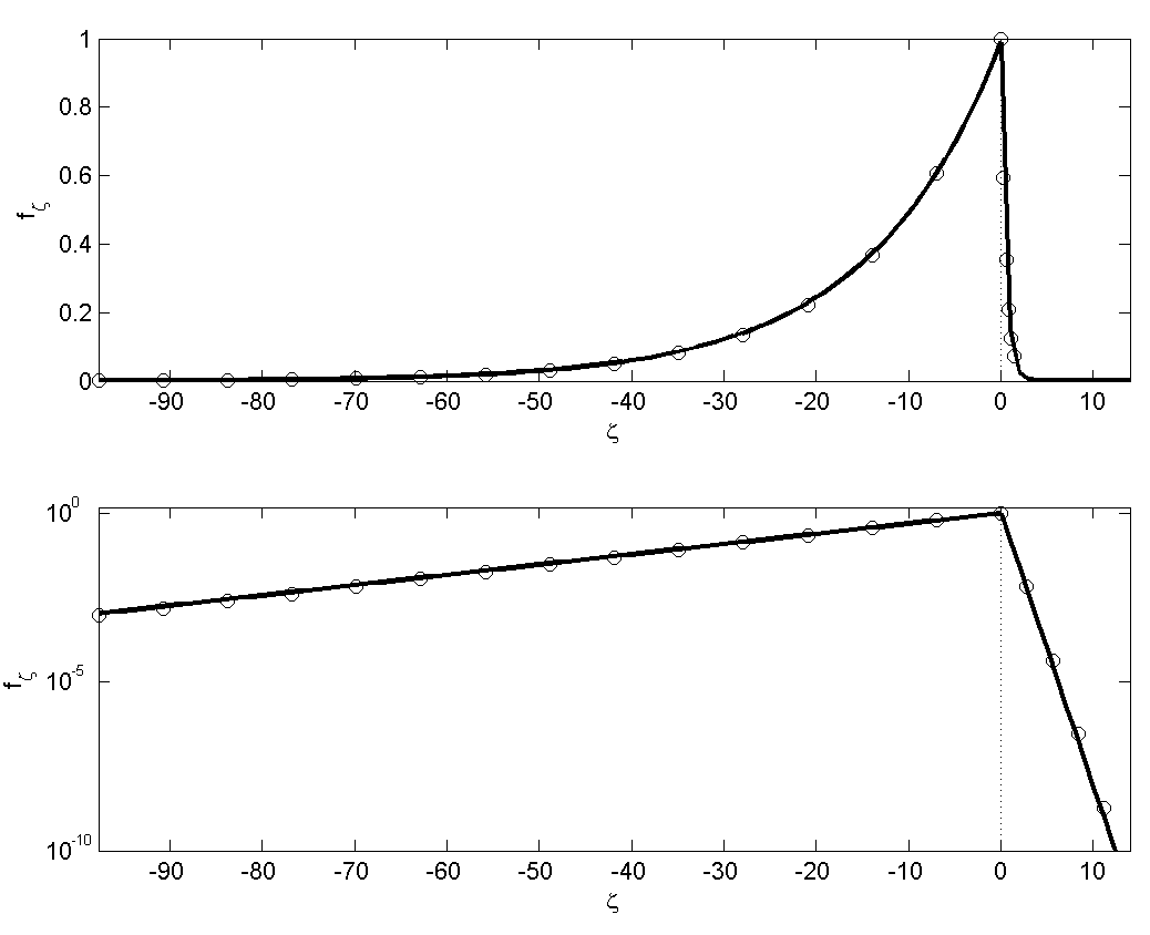
Figure 11: Simulated (solid line) and predicted (symbols) double exponential distribution of mutations obtained as a limit of the random walk with interruptions. The bottom figure shows the same distribution as the top figure but using a logarithmic ordinate.

Convergence of a random walk distribution to the double-exponential distribution is shown in Figure 11. The walk involves random steps$\ \xi=-1$ with probability 85% and $\xi=+1$ with probability 15%, while the termination parameter was set to $\lambda=0.95$. The solid line presents the numerical evaluation while the symbols show the expected double-exponential distribution. This distribution has around 4% positive mutations.

Appendix D Evolution of competitive systems

D.1 Abstract competition

Consider a large number of autonomous elements that possess two sets of properties a) non-conservative (information-like), b) conservative (energy-like) and, possibly, c) a set of physical coordinates. Abstract competition involves the following steps:

1. Selection. Random selection of elements to form competing couples, possibly with some preferences and/or isolations and possibly from the same locality in physical space.

2. Competition. Determining the winner and the loser for each couple on the basis of the element properties, possibly with some randomness.

3. Conservative mixing. The conservative properties are redistributed on even basis or from the loser to the winner. The total amounts are preserved in this redistribution.

4. Non-conservative mixing. The non-conservative properties are redistributed from the winner to the loser so that some or all non-conservative properties of the loser are lost.

5. Mutations. The redistribution of non-conservative properties may involve random changes (i.e. mutations), which are expected to be mostly detrimental to competitiveness of the elements.

It appears that the abstract competition can be naturally represented by a system of Pope particles with competitive and conservative mixing. In the present work, the conservative properties are limited to the particles themselves, i.e. each particle has the conservative property of $1.$ Particles with finite life times can be considered if needed.

D.2 Competitive pdf equation

In the presence of mutations, the evolution equation for the pdf takes the form

$$\frac{\partial f(\mathbf{y)}}{\partial t}=\gamma\left(\mathbb{M}\left(h^{+}(\mathbf{y},[f])f(\mathbf{y})\right)-h^{-}(\mathbf{y},[f])f(\mathbf{y})\right)$$ (76)

where and $\mathbb{M}$ is the mutation operator

$$\mathbb{M}\left(f(\mathbf{y})\right)=\underset{\infty}{\int}f_{\zeta}(\mathbf{y,y^{\circ})}f(\mathbf{y^{\circ})}d\mathbf{y}^{\circ},$$ (77)

$f_{\zeta}(\mathbf{y,y^{\circ})}$ is the normalised distribution of mutations originated from state $\mathbf{y}^{\circ}$ and $\gamma$ is the constant determining the overall rate of mixing. The non-homogeneous terms present in the standard pdf equation (4) are not included here since the case is presumed to be spatially homogeneous. This equation is a generalisation of the evolution equation derived in Ref. [5] and is quite transparent: $h^{+}(\mathbf{y},[f])f(\mathbf{y})$ is the total fraction of losers to the element $\mathbf{y}$ and $h^{-}(\mathbf{y},[f])f(\mathbf{y})$ is the total fraction of winners over the element $\mathbf{y}$. The losers are subject to mutations originated at $\mathbf{y}$ while the winners remove particles from location $\mathbf{y}$.

D.3 Mutation-free evolution

In the absence of mutations the rate of change of the distribution can be easily expressed in terms of relative ranking

$$\frac{\partial\ln(f(\mathbf{y))}}{\partial t}=\gamma\theta(\mathbf{y,}[f]),\;\;\;\mathbf{\zeta}=0$$ (78)

where $\gamma$ is the constant determining the rate of mixing and $\theta(\mathbf{y,}[f])=r(\mathbf{y,}[f])\psi(\mathbf{y,}[f])$. We note that the cases where there is a draw do not change the properties when mutations are not present.

In case of transitive competition of non-isolated particles, a steady state is possible only in a trivial case when all particles have the same rank (and thus $R_{pq}=0$ for any $p$ and $q$). Indeed, any particle $p$, which has a rank $r_{p}$ lower than that of the leader $r_{\ast}$, would eventually lose competition to the leader and acquire the leading rank $r_{\ast}$. The steady state is reached only when all particles are ranked at $r_{\ast}$. A steady state with $R_{pq}\neq 0$ is, however, possible for intransitive competition. For example, consider particles equally distributed between the three states in the scissors-paper-rock competition. This distribution is steady as the probabilities of losing a particle and gaining a particle are the same for all three states. Stability of non-trivial steady distributions in intransitive competitions is not guaranteed and needs to be examined.

Equation (78) indicates that in absence of mutations any stationary solution requires $\theta(\mathbf{y,}[f_{0}])=0$ for any $\mathbf{y}$ such that $f(\mathbf{y})>0$. Consider variation $\delta f(\mathbf{y})=f(\mathbf{y})-f_{0}(\mathbf{y})$, whose support is not larger than that of $f_{0}(\mathbf{y})$ (that is $\delta f(\mathbf{y})=0$  for all $\mathbf{y}$ that$\ f(\mathbf{y})=0$) then within the support of $f_{0}(\mathbf{y})$ we have $\theta(\mathbf{y},[f_{0}])=0$ and

$$\theta(\mathbf{y},[f])=\theta(\mathbf{y},[f_{0}+\delta f])=\theta(\mathbf{y},[f_{0}])+\theta(\mathbf{y},[\delta f])=\theta(\mathbf{y},[\delta f])$$ (79)

The linearised form of equation (78) is

$$\frac{\partial\delta f(\mathbf{y})}{\partial t}=\gamma f_{0}(\mathbf{y})\theta(\mathbf{y,}[\delta f])$$ (80)

With the use of $\widetilde{\delta f}(\mathbf{y})=\delta f(\mathbf{y})/f_{0}(\mathbf{y})^{1/2}$ this equation can be written as

$$\frac{\partial\widetilde{\delta f}}{\partial t}=\gamma\mathbb{L}_{f}\widetilde{\delta f}$$ (81)

where $\mathbb{L}_{f}$ is a linear operator applied to $\widetilde{\delta f}$ and defined by

$$\mathbb{L}_{f}\widetilde{\delta f}(\mathbf{y})=\underset{\infty}{\int}\Psi(\mathbf{y},\mathbf{y}^{\prime})R(\mathbf{y},\mathbf{y}^{\prime})\widetilde{\delta f}(\mathbf{y}^{\prime})\sqrt{f(\mathbf{y})f(\mathbf{y}^{\prime})}d\mathbf{y}^{\prime}$$ (82)

The positiveness of $f_{0}(\mathbf{y})$ for all $\mathbf{y}$ where $\delta f(\mathbf{y})\neq 0$ must be noted. The operator $\mathbb{L}_{f}$ is skew-symmetric (anti-symmetric)

$$\underset{\infty}{\int}\widetilde{\delta f}(\mathbf{y})\mathbb{L}_{f}\widetilde{\delta f}(\mathbf{y})d\mathbf{y}=0$$ (83)

due to $R(\mathbf{y},\mathbf{y}^{\prime})=-R(\mathbf{y}^{\prime},\mathbf{y})$. The solution of equation (81) with initial conditions  $\widetilde{\delta f}(\mathbf{y})=\widetilde{\delta f^{\circ}}(\mathbf{y})$ at $t=0$ is given by

$$\widetilde{\delta f}(\mathbf{y})=\exp(\gamma t\mathbb{L}_{f}\mathbb{)}\widetilde{\delta f^{\circ}}(\mathbf{y})$$ (84)

where the exponential operator is unitary. Hence, unless $R_{pq}=0$ for all particle couples $p$ and $q,$ the system of competing particles without mutations has non-decaying oscillations. Generally, negative mutations tend to act as a stabilising factor while positive mutations tend to be destabilising.

D.4 Nearly mutation-free evolution

Consider the overall steady distribution $f(\mathbf{y})$, represented by a superposition of $a_{I}\phi_{I}(\mathbf{y}),$ where $\phi_{I}(\mathbf{y})$ is the distribution of particles within one of the subsystems $I=1,...,K$ located in domains $\mathfrak{D}_{I}$ as specified by (45). The major changes in the system occur due to the competition between the subsystems, which does not involve mutations, while smaller adjustments of distributions happen due to competitions within each subsystem and may involve some non-positive mutations. The distribution $f(\mathbf{y})$ is, initially, at equilibrium.

If competition is transitive and the subsystem leaders $\mathbf{y}_{I\ast}$ are not isolated from each other, then any non-trivial steady distribution is impossible. Indeed, once a subsystem leader has lost competition to a leader from another subsystem, it cannot be replaced due to absence of mutations between subsystems and absence of positive mutations within the subsystem. The system keeps evolving until only one subsystem is left. A non-trivial steady state, however, is possible in intransitive competition.

Let us consider linear stability of the equilibrium with respect to the disturbance, which is represented by small changes in $a_{I}$ while $\phi_{I}(\mathbf{y})$ are not changed initially and remain the same within accuracy of our analysis. In the absence of mutational exchanges between the subsystem, this leads to the relation

$$\frac{\partial a_{I}}{\partial t}=\gamma\bar{\Theta}_{I}([f])a_{I}=\gamma\sum_{J}a_{I}a_{J}\bar{\Theta}_{IJ}$$ (85)

which can be obtained from (76) by integrating $f$ over each of the subsystem domains $\mathfrak{D}_{I}$ under assumptions that $\phi_{I}(\mathbf{y})$ (and consequently $\bar{\Theta}_{IJ})$ are at equilibrium and do not change in time and that domains $\mathfrak{D}_{I}$ do not exchange mutations.

Since $f(\mathbf{y})$ is steady, equation (85) indicates that $\bar{\Theta}_{I}a_{I}=0$. We investigate stability of the system with respect to changes of every $a_{I}\neq 0$ and $\bar{\Theta}_{I}=0$ by $\Delta a_{I}$ assuming that $\phi_{I}(\mathbf{y})$ do not change that is $\Delta f(\mathbf{y})=\Sigma_{I}\phi_{I}(\mathbf{y})\Delta a_{I}.$ Note that if $a_{J}=0$, competition without mutations does not allow to change this value. Equation (85) takes the form

$$\frac{\partial a_{I}}{\partial t}=\gamma a_{I}\Delta\bar{\Theta}_{I}=\gamma a_{I}\sum_{J=1}^{K}\bar{\Theta}_{IJ}\Delta a_{J}$$ (86)

With $\widetilde{\Delta a}_{I}=\Delta a_{I}/a_{I}^{1/2}$ the linearised version of this equation takes the form

$$\frac{\partial\widetilde{\Delta a}_{I}}{\partial t}=\sum_{J=1}^{K}L_{IJ}\widetilde{\Delta a}_{J}=\mathbb{L}_{a}\widetilde{\Delta a}_{I}$$ (87)

where the linear operator $\mathbb{L}_{a}$ is represented by the skew-symmetric matrix

$$L_{IJ}=a_{I}^{1/2}\bar{\Theta}_{IJ}a_{J}^{1/2}$$ (88)

Note that $a_{I}>0$ for any $I$ that $\Delta a_{I}>0$. The solution of equation (87) with initial conditions $\widetilde{\Delta a}_{I}=\widetilde{\Delta a_{I}^{\circ}}$ at $t=0$ is

$$\widetilde{\Delta a}_{I}=\sum_{J=1}^{K}\exp(\gamma t\mathbb{L}_{a})\widetilde{\Delta a_{I}^{\circ}}$$ (89)

where the matrix exponent $\exp(\gamma t\mathbb{L}_{a})$ produces a unitary matrix. Hence, unless $\bar{\Theta}_{IJ}=\bar{R}_{IJ}\bar{\Psi}_{IJ}=0$ for every $I$ and $J,$ a deviation from the steady state is expected to generate oscillations in the system. Equilibration of two non-isolated subsystems $I$ and $J$ in the absence of mutational exchanges between the subsystems needs $\bar{R}_{IJ}=0$ rather than equivalence of the competitive potentials.

D.5 Competitive H-theorem

The competition considered here can be transitive or intransitive, preferential or non-preferential. Mutations are represented by Gibbs mutations satisfying formula (54).

Theorem 1

The total entropy of a competitive system with non-positive Gibbs mutations monotonically increases during evolution of the system until it reaches its maximal value at the equilibrium.

For mutations distributed according to equation (54), the governing equation (76) takes the form

$$\frac{\partial f(\mathbf{y}_{1})}{\partial t}=$$

$$\gamma\underset{\infty}{\int}H(\mathbf{y}_{2},\mathbf{y}_{1})\Psi(\mathbf{y}_{1},\mathbf{y}_{2})\frac{f(\mathbf{y}_{2})}{h_{0}^{+}(\mathbf{y}_{2})}\left(f_{0}(\mathbf{y}_{1})h^{+}(\mathbf{y}_{2},[f])-f(\mathbf{y}_{1})h_{0}^{+}(\mathbf{y}_{2})\right)d\mathbf{y}_{2}$$

$$=\gamma\underset{\infty}{\int\int}\Phi_{3}(\mathbf{y}_{1},\mathbf{y}_{2},\mathbf{y}_{3})\underset{\varphi(\mathbf{y}_{1},\mathbf{y}_{3})}{\underbrace{\left(f_{0}(\mathbf{y}_{1})f(\mathbf{y}_{3})-f(\mathbf{y}_{1})f_{0}(\mathbf{y}_{3})\right)}}d\mathbf{y}_{3}d\mathbf{y}_{2}$$ (90)

where

$$\Phi_{3}(\mathbf{y}_{1},\mathbf{y}_{2},\mathbf{y}_{3})=H(\mathbf{y}_{2},\mathbf{y}_{1})\Psi(\mathbf{y}_{1},\mathbf{y}_{2})H(\mathbf{y}_{2},\mathbf{y}_{3})\Psi(\mathbf{y}_{3},\mathbf{y}_{2})\frac{f(\mathbf{y}_{2})}{h_{0}^{+}(\mathbf{y}_{2})}\geq 0$$

Evaluation of the time derivative for the entropy defined by

$$S([f(\mathbf{y})])=\;-\int_{\infty}f(\mathbf{y})\ln\left(\frac{f(\mathbf{y})}{f_{0}(\mathbf{y})}\right)d\mathbf{y+}C_{0}([f_{0}(\mathbf{y})])$$ (91)

results, after substitution of (90), in

$$\frac{dS}{dt}=-\underset{\infty}{\int}\frac{\partial f(\mathbf{y}_{1})}{\partial t}\ln\left(\frac{f(\mathbf{y}_{1})}{f_{0}(\mathbf{y}_{1})}\right)d\mathbf{y}_{1}=$$

$$-\gamma\underset{\infty}{\int\int\int}\Phi_{3}(\mathbf{y}_{1},\mathbf{y}_{2},\mathbf{y}_{3})\underset{\Phi_{2}(\mathbf{y}_{1},\mathbf{y}_{3})}{\underbrace{\varphi(\mathbf{y}_{1},\mathbf{y}_{3})\ln\left(\frac{f(\mathbf{y}_{1})}{f_{0}(\mathbf{y}_{1})}\right)}}d\mathbf{y}_{1}d\mathbf{y}_{2}d\mathbf{y}_{3}=$$

$$-\gamma\underset{\infty}{\int\int\int}\Phi_{3}(\mathbf{y}_{1},\mathbf{y}_{2},\mathbf{y}_{3})\frac{\Phi_{2}(\mathbf{y}_{1},\mathbf{y}_{3})+\Phi_{2}(\mathbf{y}_{3},\mathbf{y}_{1})}{2}d\mathbf{y}_{1}d\mathbf{y}_{2}d\mathbf{y}_{3}$$ (92)

Here, we use the symmetric properties $\Phi_{3}(\mathbf{y}_{1},\mathbf{y}_{2},\mathbf{y}_{3})=\Phi_{3}(\mathbf{y}_{3},\mathbf{y}_{2},\mathbf{y}_{1})$ of the function $\Phi_{3}$ while noting that the variables $\mathbf{y}_{1}$ and $\mathbf{y}_{3}$ are dummy integration variables and can be swapped in the integral. With the use the expression

$$\Phi_{2}(\mathbf{y}_{1},\mathbf{y}_{3})+\Phi_{2}(\mathbf{y}_{3},\mathbf{y}_{1})=$$

$$\varphi(\mathbf{y}_{1},\mathbf{y}_{3})\left(\ln\left(\frac{f(\mathbf{y}_{1})}{f_{0}(\mathbf{y}_{1})}\right)-\ln\left(\frac{f(\mathbf{y}_{3})}{f_{0}(\mathbf{y}_{3})}\right)\right)=$$

$$-f_{0}(\mathbf{y}_{1})f(\mathbf{y}_{3})\left(\omega-1\right)\ln(\omega)\leq 0$$ (93)

and antisymmetry of the function $\varphi$

$$\varphi(\mathbf{y}_{1},\mathbf{y}_{3})=-\varphi(\mathbf{y}_{3},\mathbf{y}_{1})$$

while introducing $\omega$ by

$$\omega=\frac{f(\mathbf{y}_{3})}{f_{0}(\mathbf{y}_{3})}\frac{f_{0}(\mathbf{y}_{1})}{f(\mathbf{y}_{1})}$$

and noting that $\left(\omega-1\right)\ln(\omega)\geq 0,$ we obtain the relation

$$\frac{\gamma}{2}\underset{\infty}{\int\int\int}\Phi_{3}(\mathbf{y}_{1},\mathbf{y}_{2},\mathbf{y}_{3})f_{0}(\mathbf{y}_{1})f(\mathbf{y}_{3})\left(\omega-1\right)\ln(\omega)d\mathbf{y}_{1}d\mathbf{y}_{2}d\mathbf{y}_{3}=$$

$$=\frac{dS}{dt}\geq 0$$ (94)

proving the H-theorem.

D.6 Convergence theorem for transitive competition

The mutations considered in this subsection are deemed to be general non-positive mutations (rather than Gibbs mutations), although our analysis is restricted to transitive competition. Consider competition within a closed domain $\mathfrak{D}$ that has a finite measure (i.e. volume) $\mu(\mathfrak{D})<\infty$ and assume that the mutation distribution function $f_{\zeta}(\mathbf{y},\mathbf{y}^{\circ})$ is continuous in this domain. The mixing is assumed to be non-preferential ($\Psi=1$). The absolute ranking $r_{\#}(\mathbf{y})$ is continuous and satisfies additional continuity requirement $\mu(\mathfrak{D}_{2}(r_{1},r_{1}+\Delta r))\rightarrow 0$ as $\Delta r\rightarrow 0$ uniformly in $\mathfrak{D.}$ Here we define $\ \mathfrak{D}_{2}(r_{1},r_{2})=\{\mathbf{y|}r_{1}\mathbf{\leq}r_{\#}(\mathbf{y})\mathbf{\leq}r_{2}\}$ and, analogously, $\mathfrak{D}_{2}(\mathbf{y}_{1}\mathbf{,y}_{2})=\{\mathbf{y}|\mathbf{y}_{1}\mathbf{\preccurlyeq y\preccurlyeq y}_{2}\}.$ For the mathematical space of continuous functions $f(\mathbf{y})$ defined on $\mathfrak{D}$ and conventionally denoted by $C^{0}(\mathfrak{D),}$ the norm of $f$ can be specified by

$$\left\|f\right\|=\max_{\mathbf{y}\in\mathfrak{D}}\left(\left|f(\mathbf{y})\right|\right)$$ (95)

The mathematical restrictions considered here are introduced to keep the proof transparent and, in principle, can be modified or relaxed.

Theorem 2

If competition is transitive and mutations are non-positive, the system asymptotically approaches its equilibrium state where the total entropy of the system reaches its maximal value.

If mutations are non-positive, the governing equation (76) takes the form

$$\frac{\partial f(\mathbf{y})}{\partial t}=$$

$$\gamma\underset{\mathfrak{D}}{\int}H(\mathbf{y}^{\circ},\mathbf{y})\left(f_{\zeta}(\mathbf{y},\mathbf{y}^{\circ})(1-h^{-}(\mathbf{y}^{\circ},[f]))-f(\mathbf{y})\right)f(\mathbf{y}^{\circ})d\mathbf{y}^{\circ}$$ (96)

implying that for any $\mathbf{y}_{1}$ the evolution of the distribution in the region $\mathbf{y}\succcurlyeq\mathbf{y}_{1}$ does not depend on the distribution in the region $\mathbf{y\prec y}_{1}$. If a stationary solution is reached for $\mathbf{y}\succcurlyeq\mathbf{y}_{1},$ it will remain in this state although $f(\mathbf{y})$ may still evolve at $\mathbf{y\prec y}_{1}$. we can formally rewrite equation (96) in the form

$$\frac{\partial f(\mathbf{y)}}{\partial t}=\int_{\mathbf{y}}^{\mathbf{y}_{\ast}}f_{\zeta}(\mathbf{y,y}^{\circ}\mathbf{)}\left(1-h^{-}(\mathbf{y}^{\circ},[f])\right)f(\mathbf{y}^{\circ})d\mathbf{y}^{\circ}$$

$$-h^{-}(\mathbf{y},[f])f(\mathbf{y})$$ (97)

where

$$h^{-}(\mathbf{y,[}f])=\int_{\mathbf{y}}^{\mathbf{y}_{\ast}}f(\mathbf{y}^{\circ})d\mathbf{y}^{\circ}$$ (98)

The limits in this equation imply that the integral is evaluated over the region $\mathfrak{D}_{2}(\mathbf{y,y}_{\ast})$ where $\mathbf{y}_{\ast}$ is the location of the leading particle. Note that the regions $\mathfrak{D}_{2}(\mathbf{y}_{1}\mathbf{,y}_{1})$ have a zero measure for any $\mathbf{y}_{1}$.

If the steady solution is established in the region $\mathfrak{D}_{2}(\mathbf{y}_{1}\mathbf{,y}_{\ast})$ but not in the region $\mathfrak{D}_{2}(\mathbf{y,y}_{1}),$ which is presumed to be small as $\mathbf{y}$ is taken close to $\mathbf{y}_{1},$ a steady state must be established in the second region as it is effectively controlled by the first region and mutations in a small region can always be deemed close to being Gibbs mutations.

The integral in (97) can be divided into several terms

$$\frac{\partial f}{\partial t}=\gamma Q_{0}+\gamma\mathbb{Q}_{1}(f)-\gamma\mathbb{Q}_{2}(f)-\gamma h_{0}^{-}(\mathbf{y}_{1})f(\mathbf{y})$$ (99)

where

$$Q_{0}=\int_{\mathbf{y}_{1}}^{\mathbf{y}_{\ast}}f_{\zeta}(\mathbf{y,y}^{\circ}\mathbf{)(}1\mathbf{-}h_{0}^{-}(\mathbf{y}^{\circ}))f_{0}(\mathbf{y}^{\circ})d\mathbf{y}^{\circ}$$

$$\mathbb{Q}_{1}(f)=\int_{\mathbf{y}}^{\mathbf{y}_{1}}f_{\zeta}(\mathbf{y,y}^{\circ}\mathbf{)}(1-h^{-}(\mathbf{y}^{\circ},[f]))f(\mathbf{y}^{\circ})d\mathbf{y}^{\circ}$$

$$\mathbb{Q}_{2}(f)=f(\mathbf{y})\left(h^{-}(\mathbf{y},[f])-h_{0}^{-}(\mathbf{y}_{1})\right)=f(\mathbf{y})\int_{\mathbf{y}}^{\mathbf{y}_{1}}f(\mathbf{y}^{\circ})d\mathbf{y}^{\circ}$$

and seek a solution in form of the time steps

$$f(\mathbf{y},t+\Delta t)=$$

$$f(\mathbf{y},t)\left(1-h_{0}^{-}(\mathbf{y}_{1})\gamma\Delta t\right)+\gamma\Delta t\left(Q_{0}+\mathbb{Q}_{1}(f)-\mathbb{Q}_{2}(f)\right)$$ (100)

The norms of the operators $\mathbb{Q}_{1}$ and $\mathbb{Q}_{2}$ can be easily estimated by

$$\left\|\mathbb{Q}_{1}\right\|\leq\left\|f_{\zeta}\right\|_{\Delta}\mu_{\Delta}$$

$$\left\|\mathbb{Q}_{2}\right\|\leq 2\left\|f\right\|_{\Delta}\mu_{\Delta}$$

where

$$\mu_{\Delta}=\mu(\mathfrak{D}_{2}(\mathbf{y,y}_{1}))$$

is the measure of the region $\mathfrak{D}_{2}(\mathbf{y,y}_{1})$ and the norms subscribed by $\Delta$ are evaluated over $\mathfrak{D}_{2}(\mathbf{y,y}_{1})$. The norm of operators $\mathbb{Q}_{1}$ and $\mathbb{Q}_{2}$ can be made smaller than any given $\varepsilon>0$ by selecting $r_{\#}(\mathbf{y)}$ sufficiently close to (but still at a finite distance from) $r_{\#}(\mathbf{y}_{1}).$  The leading order estimate of the stationary distribution on $\mathfrak{D}_{2}(\mathbf{y,y}_{1})$ is given by $f_{0}\approx Q_{0}/h_{0}^{-}(\mathbf{y}_{1}),$ constraining the norms of the converging distributions (assuming reasonable initial conditions). Since $Q_{0}$ does not depend on $f$ and the norms of the operators $\mathbb{Q}_{1}$ and $\mathbb{Q}_{2}$ are relatively small, the operator on the right-hand side of equation (D.25) becomes a contraction mapping (provided $\varepsilon$ is selected so that $\varepsilon<h_{0}^{-}(\mathbf{y}_{1})$ and the time step $\Delta t$ is sufficiently small). This proves convergence and uniqueness of the solution.

Note that $\varepsilon$ can be selected uniformly over the domain with the exception of the vicinity of the leading particle where $h_{0}^{-}(\mathbf{y})\rightarrow 0$ as $\mathbf{y\rightarrow y}_{\ast}$.  One may also notice that $\partial f(\mathbf{y)/}\partial t\rightarrow 0$ as $\mathbf{y\rightarrow y}_{\ast}$. The vicinity of leading particle needs special consideration that takes into account the discrete nature of the particle system. The position of the leading particle is fixed and we need to consider the distribution behind the leading particle where $h_{0}^{-}(\mathbf{y})\geq 1/n$ is positive, where $n$ is the total number of particles. The singularity of $h_{0}^{-}(\mathbf{y})\rightarrow 0$ as $\mathbf{y\rightarrow y}_{\ast}$ indicates that convergence to a steady solution in the leading group is not uniform and can be quite slow. Indeed, let two particles $p$ and $q$ be initially located at $\mathbf{y}_{\ast}.$ This distribution is not at equilibrium since eventually, after certain characteristic time $t_{\ast},$ these two particles would form a mixing couple and one of them is destined to leave the leading position. If the total number of particles $n$ is very large, the deviation from the equilibrium is small but the time $t_{\ast}$ can be very large.

As $f\rightarrow f_{0}$, the entropy defined by (91) approaches its maximal value; the theorem, however, does not guarantee that this process is monotonic.

Figure 6: Intransitivity of energy exchange between Reynolds stresses in turbulent shear flows

Figure 7: Intransitivity of the Oregonator model [83] for the Belousov-Zhabotinsky reaction.

Figure 9: Average intensity of colours indicating leaping cycles, average relative rank $\bar{R}_{u}$, configurational entropy $S_{c}$ and average intensity of competition $\Xi$ indicating the level of competitive cooperation in intransitive abstract competition. The vertical dashed line shows location of images displayed in the next Figure.

Figure 10: Order appearing out of chaos: the red spot gradually asserts its dominance over the domain that previously was in a state of chaos. The blue spot on the left attempts to launch a competitive bid for dominance but ultimately fails. Two consecutive frames of this process are shown. The property space is shown in the left column of figures while corresponding physical spaces are shown in the right column.

References

- [1] G. Nicolis and I. Prigogine. Self-organization in nonequilibrium systems: from dissipative structures to order through fluctuations. Wiley, New York, 1977.
- [2] R. Kindermann and J. L. Snell. Markov random fields and their applications. AMS, 1980.
- [3] E. H. Lieb and J. Yngvason. The entropy of classical thermodynamics. In A. Greven, G. Keller, and G. Warnecke, editors, Entropy, chapter 8, pages 147–195. Princeton University Press, 2003.
- [4] C. Caratheodory. Studies in the foundation of thermodynamics. Math. Ann., 67:355 386, 1909.
- [5] A. Y. Klimenko. Conservative and competitive mixing and their applications. Physica Scripta, T142:014054, 2010.
- [6] A. Y. Klimenko and S. B. Pope. Propagation speed of combustion and invasion waves in stochastic simulations with competitive mixing. Combustion Theory and Modelling, page doi:10.1080/13647830.2011.647091, 2012.
- [7] N. de Condorcet. Essay on the Application of Analysis to the Probability of Majority Decisions. De L’imprimerie Royale., Paris, 1785.
- [8] S. B. Pope. Pdf methods for turbulent reactive flows. Prog. Energy Combust. Sci., 11:119–192, 1985.
- [9] F. A. Williams. Combustion Theory. Addison-Wesley, Reading, MA, 2nd edition, 1985.
- [10] V. R. Kuznetsov and V. A. Sabelnikov. Turbulence and Combustion. Hemisphere, New York, 1990.
- [11] J. Warnatz, U. Maas, and R. W. Dibble. Combustion: physical and chemical fundamentals, modelling and simulation, experiments, pollutant formation. Springer-Verlag, Berlin, 1996.
- [12] A. Y. Klimenko and R. W. Bilger. Conditional moment closure for turbulent combustion. Prog. Energy Combust. Sci., 25:595–687, 1999.
- [13] S. B. Pope. Turbulent Flows. Cambridge University Press, Cambridge, 2000.
- [14] R. Fox. Computational Models for Turbulent Reacting Flows. Cambridge University Press, Cambridge, 2003.
- [15] S. Heinz. Statistical Mechanics of Turbulent Flows. Springer, Berlin, 2003.
- [16] H. Pitsch. Large-Eddy simulations of turbulent combustion. Annu. Rev. Fluid Mech., 38:453–482, 2006.
- [17] D. Haworth. Progress in probability density function methods for turbulent reacting flows. Prog. Energy Combust. Sci., 36:168–259, 2010.
- [18] T. Echekki and E. Mastorakos. Turbulent Combustion Modelling. Advances, New Trends and Perspectives. Springer, 2011.
- [19] A. Y. Klimenko and M. J. Cleary. Convergence to a model in sparse-lagrangian fdf simulations. Flow, Turbulence and Combustion (Special issue dedicated to S.B.Pope), 85:567 591, 2010.
- [20] S. Devine. The insights of algorithmic entropy. Entropy, 11(1):85–110, 2009.
- [21] M. Gell-Mann. The quark and the jaguar. W.H.Freemen and Co., N.-Y., 1994.
- [22] J.H. Holland. Studying complex adaptive systems. J. of Syst. Sci. and Complexity, 19(1):1–8, 2006.
- [23] F. Heylighen, J. Bollen, and A. Riegler. The evolution of complexity, volume 8. Kluwer, Dordrecht, 1999.
- [24] P. Glansdorff and I. Prigogine. Thermodynamic theory of structure, stability and fluctuations. Wiley-Interscience, London ; New York, 1971.
- [25] G. W. Paltridge. Climate and thermodynamic systems of maximum dissipation. Nature, 279(5714):630–631, 1979.
- [26] H. Ziegler. An introduction to thermomechanics, volume 21. North-Holland, Amsterdam ; New York, 1983.
- [27] D.J. Evans and D.J. Searles. The fluctuation theorem. Advances in Physics, 51(7):1529–1585, 2002.
- [28] L. M. Martyushev and V. D. Seleznev. Maximum entropy production principle in physics, chemistry and biology. Physics Reports, 426(1):1–45, 2006.
- [29] R. Swenson. The fourth law of thermodynamics or the law of maximum entropy production. Chemistry, 18(5):333–339, 2009.
- [30] S. B. Pope. A rational method of determining probability distributions in turbulent reacting flows. J. Non-Equilib. Thermodyn, 4:309–320, 1979.
- [31] T. H. Dupree. Coarse-grain entropy in two-dimensional turbulence. Physics of Fluids B: Plasma Physics, 4(10):3101, 1992.
- [32] P. Sancho and J. Llebot. Thermodynamic entropy and turbulence. Physica A: Statistical and Theoretical Physics, 205(4):623–633, 1994.
- [33] G. Falkovich and A. Fouxon. Entropy production and extraction in dynamical systems and turbulence. New Journal of Physics, 6:50–50, 2004.
- [34] A. Celani and A. Seminara. Large-scale structure of passive scalar turbulence. Phys. Rev. Lett., 94(21):214503–214503, 2005.
- [35] A. Gray-Weale and P. Attard. Time correlations and the second entropy. The Journal of Chemical Physics, 127:044503, 2007.
- [36] J. Duplat and E. Villermaux. Mixing by random stirring in confined mixtures. J. Fluid Mech., 617:51–86, 2008.
- [37] C.E. Shannon. Prediction and entropy of printed english. Bell System Technical Journal, 30(1):50–64, 1951.
- [38] D. N. Saulov, I. G. Vladimirov, and A.Y. Klimenko. Modified associate formalism without entropy paradox: Part I. model description. Journal of Alloys and Compounds, 473(1-2):167 – 175, 2009.
- [39] A. Y. Klimenko. Lagrangian particles with mixing. I. simulating scalar transport. Phys. Fluids, 21:065101, 2009.
- [40] A. Y. Klimenko and S. B. Pope. A model for turbulent reactive flows based on multiple mapping conditioning. Physics of Fluids, 15:1907–1925, 2003.
- [41] M.J. Cleary and A.Y. Klimenko. Multiple mapping conditioning: a new modelling framework for turbulent combustion. In T. Echekki and E. Mastorakos, editors, Turbulent Combustion Modelling. Advances, New Trends and Perspectives., chapter 7, pages 143–173. Springer, 2011.
- [42] G. van Heijst, R. Trieling, M. Hoeijmakers, F. Fontenele Araujo, and H. Nijmeijer. Control of mixing via entropy tracking. Physical Review E, 81(6):066302, 2010.
- [43] A. Garrid. About some properties of the Kullback-Leibler divergence. Advanced Modeling and Optimization, 11:571–578, 2009.
- [44] V. S. Lvov. Spectra of velocity and temperature-fluctuations with constant entropy flux of fully-developed free-convective turbulence. Phys. Rev. Lett., 67(6):687–690, 1991.
- [45] Z. Ren and S. B. Pope. Entropy production and element conservation in the quasi-steady-state approximation. Combustion and Flame, 137(1-2):251–254, 2004.
- [46] V. Scherer, S. Wirtz, and J. Leicher. Evaluation of an entropy-based combustion model using stochastic reactors. Chemical Engineering and Technology, 31(7):964–970, 2008.
- [47] V. Bykov and U. Maas. Reaction-diffusion manifolds and global quasi-linearization: Two complementary methods for mechanism reduction. The Open Thermodynamics Journal, 4:92–100, 2010.
- [48] J. Whitfield. Order out of chaos. Nature, 436(7053):905–907, 2005.
- [49] H. Sakuma, S. Shimokawa, and H. Ozawa. Thermodynamics of fluid turbulence: a unified approach to the maximum transport properties. Physical review. E, 64(2 Pt 2):026303, 2001.
- [50] J. Sommeria. Entropy production in turbulent mixing. In M Lesieur, A. Yaglom, and F. David, editors, New trends in turbulence, pages 79–91. Springer Berlin Heidelberg, Berlin, Heidelberg, 2005.
- [51] C. Dopazo. Probability density function approach for a turbulent axisymmetric heated jet centreline evolution. Phys. Fluids, 18:397–410, 1975.
- [52] R. L. Curl. Dispersed phase mixing. I. AIChE J., 9:175, 1963.
- [53] J. Janicka, W. Kolbe, and W. Kollmann. Closure of the transport equation for the probability density function of scalar fields. J. Non-equilib. Thermodyn, 4(1):47–66, 1979.
- [54] R. P. Lindstedt, S. A. Louloudi, J. J. Driscoll, and V. Sick. Finite rate chemistry effects in turbulent reacting flows. Flow, Turbulence and Combustion, 72:407–426, 2004.
- [55] S. Subramaniam and S. B. Pope. A mixing model for turbulent reactive flows based on Euclidean minimum spanning trees. Combust. Flame, 115:487–514, 1998.
- [56] H. Chen, S. Chen, and R. H. Kraichnan. Probability distribution of a stochastically advected scalar field. Phys. Rev. Lett., 63:2657–2660, 1989.
- [57] S. B. Pope. Mapping closures for turbulent mixing and reaction. Theor. Comput. Fluid Dyn., 2:255–270, 1991.
- [58] A. Y. Klimenko. Computer simulations of abstract competition. In Proceedings of International Conference on Complexity, Informatics and Cybernetics (IMCIC), volume 1, pages 97–102, 2010.
- [59] S. B. Pope and M. S. Anand. Flamelet and distributed combustion in premixed turbulent flames. In Proc. Combust. Inst, volume 20, pages 403–410, Pittsburgh, 1985. Combustion Institute.
- [60] A. N. Kolmogorov, I. G. Petrovsky, and N. S. Piskunov. A study of the equation of diffusion with increase in the quantity of matter, and its application to a biological problem. Mosc. Univ. Bull. (A: Math. and Mech.), 1:1, 1937.
- [61] R. A. Fisher. The wave of advance of advantageous genes. Ann. Eugen., 7:355, 1937.
- [62] K. N. C. Bray, P. A. Libby, and J. B. Moss. Flamelet crossing frequencies and mean reaction rates in premixed turbulent combustion. Combust. Sci. Technol., 41:143–172, 1984.
- [63] M. Eigen. Selforganization of matter and the evolution of biological macromolecules. Naturwissenschaften, 58:465–523, 1971.
- [64] R. Giles. Mathematical foundations of thermodynamics. Pergamon, Oxford, 1964.
- [65] J. L. B. Cooper. The foundations of thermodynamics. Journal of Mathematical Analysis and Applications, 17:172 193, 1967.
- [66] H. A. Buchdahl. Twenty lectures on thermodynamics. Pergamon Press (Australia), 1975.
- [67] P. T. Landsberg. Thermodynamics and statistical mechanics. Oxford University Press, Oxford, 1978.
- [68] A. Thess. The Entropy Principle. Springer, Dordrecht, 2011.
- [69] G. Debreu. Presentation of a preference odering by a numerical function. In R. M. Thrall, C. H. Coombs, and R. L. Davis, editors, Decision process, pages 159–165. J.Wiley and Sons, 1954.
- [70] G. B. Mehta. Preference and utility. In S. Barbera, P. Hammond, and C. Seidl, editors, Handbook of utility theory, pages 1 –47. Kluwer, Boston, 1999.
- [71] J. C. Candeal, J. R. De Miguel, E. Indurain, and G.B. Mehta. Utility and entropy. Economic Theory, 17(1):233–238, 2001.
- [72] T. Ohta. Extension to the neutral mutation random drift hypothesis. In M Kimura, editor, Molecular Evolution and Polymorphism, pages 148 –167. National Institute of Genetics, Mishima, 1977.
- [73] D. Bouyssou. Monotonicity of ranking by choosing : A progress report. Social Choice and Welfare, 23(2):249–273, 2004.
- [74] G. Slutzki and O. Volij. Ranking participants in generalized tournaments. International Journal of Game Theory, 33(2):255–270, 2005.
- [75] R.-R. Joseph. Making choices with a binary relation: Relative choice axioms and transitive closures. European Journal of Operational Research, 207(2):865–877, 2010.
- [76] G. Tullock. The irrationality of intransitivity. Oxford Economic Papers, 16(3):401–406, 1964.
- [77] K. J. Arrow. Social Choice and Individual Values. Yale University Press, USA, 1951.
- [78] David C. McGarvey. Theorem on the construction of voting paradoxes. Econometrica, 21(4):608–610, 1953.
- [79] P. Anand. The philosophy of intransitive preference. Economic Journal, 103(417):337–346, 1993.
- [80] M. Makowski and E. W. Piotrowski. Decisions in elections – transitive or intransitive quantum preferences. Journal of Physics A: Mathematical and Theoretical, 44(21):215303, 2011.
- [81] Lynne Boddy. Interspecific combative interactions between wood-decaying basidiomycetes. FEMS Microbiology Ecology, 31(3):185–194, 2000.
- [82] E. Schrodinger. What is Life - the Physical Aspect of the Living Cell. Cambridge University Press, Cambridge, UK, 1944.
- [83] R. J. Field. Limit cycle oscillations in the reversible oregonator. The Journal of Chemical Physics, 63(6):2289, 1975.
- [84] G. Debreu. Continuity properties of paretian utility. International Economic Review, 5:285 –293, 1964.
- [85] E.P. Gyftopoulos and G.P. Beretta. Thermodynamics. Foundations and Applications. Macmillan, N.Y., USA, 1991.
- [86] GJF Heijst, van, D. Molenaar, Z. Yin, and HJH Clercx. Attractor crisis and bursting in a fluid flow with two no-slip directions. Physical Review E, 75(3):036309, 2007.
- [87] J. Sommeria. Entropy production in turbulent mixing. In M Lesieur, A. Yaglom, and F. David, editors, New trends in turbulence, pages 385–447. EDP Sciences, Berlin, Heidelberg, 2001.