Amplitude death phenomena in delay–coupled Hamiltonian systems

Abstract

Hamiltonian systems, when coupled via time–delayed interactions, do not remain conservative. In the uncoupled system, the motion can typically be periodic, quasiperiodic or chaotic. This changes drastically when delay coupling is introduced since now attractors can be created in the phase space. In particular for sufficiently strong coupling there can be amplitude death (AD), namely the stabilization of point attractors and the cessation of oscillatory motion. The approach to the state of AD or oscillation death is also accompanied by a phase–flip in the transient dynamics. A discussion and analysis of the phenomenology is made through an application to the specific cases of harmonic as well as anharmonic coupled oscillators, in particular the Hénon-Heiles system.

I Introduction

The coupling between dynamical systems can give rise to a number of collective phenomena such as synchronization, phase locking, phase shifting sync , amplitude death yam ; eli ; ins ; resmi ; rep , phase-flip pf ; pfb ; nirmal , hysteresis hys , riddling rid and so on gen . Since communication between the individual systems is mediated by signals that can have a finite transmission time, many studies account for this by the introduction of time–delay in the coupling wagner ; konishi ; reddyall ; zou ; ravi ; senthil . A number of recent studies have examined the manner in which delay coupling can affect the collective dynamics, particularly since time–delay makes the systems effectively infinite dimensional farmer .

When conservative systems are coupled via time–delayed interactions, then there are additional considerations. To start with, the system becomes explicitly non–conservative and thus the nature of the dynamics changes drastically: in the uncoupled system, the phase flow preserves volumes tabor , but in the coupled system there can be attractors. This issue is of added interest when studying Hamiltonian systems where there can be a hierarchy of conserved quantities arnold . Studies of coupled Hamiltonian systems have largely examined the case of instantaneous coupling zanette which does not affect the Hamiltonian structure.

In the present work we study time–delay coupled Hamiltonian systems and examine the effect of interaction on the nature of the dynamics. We consider the following examples, that of diffusively coupled harmonic oscillators that models delay–coupled pendulums, for instance, and coupled Hénon–Heiles oscillators. In the absence of coupling, in the former case the motion is periodic, while in the latter case the dynamics can be (quasi)periodic or chaotic. In both instances we find that the effect of introducing dissipation is to cause the oscillatory dynamics to be damped to a fixed point, namely we find that there is the so–called amplitude death (AD) rep as has been seen in delay–coupled dissipative dynamical systems rep ; reddyall .

Although the major effect of the coupling is to make the overall system dissipative, there are differences from the case when non-Hamiltonian systems are coupled. When the dynamics is decaying to a point attractor, there is an abrupt transition in the relative phases of the oscillatory transient motion. This is the phase–flip transition that has been seen in a number of other systems nirmal . Here, however, there are special values of the time–delay when the coupling term effectively vanishes: the underlying Hamiltonian structure then becomes apparent.

Our main results are presented in Sections II and III where we consider the cases of coupled harmonic oscillators and coupled Hénon Heiles systems respectively. We show how AD is reached and the nature of the phase-flip transition in both cases. Since the uncoupled systems are Hamiltonian, it is possible to define an energy, and while this quantity has been studied in coupled feedback oscillators wang as a tool to determine onset of AD, its variation in the AD regime itself has not been examined. In this work we do energy analysis in the AD region and find that the energy dissipation is non monotonic as a function of the coupling, decaying faster prior to the phase–flip transition and slower subsequently. The paper concludes in Section IV with a summary and discussion of the results.

II Delay coupled harmonic oscillators

The simplest system we consider is that of diffusively coupled harmonic oscillators. We consider the following equations of motion

$$\ddot{x}_{j}+\omega_{j}^{2}x_{j}-\epsilon[\dot{x}_{k}(t-\tau)-\dot{x}_{j}(t)]=0$$ (1)

where $j,k$=1, 2 and $j\neq k$ and $x_{j}$ and $\dot{x}_{j}$ represent the position and the velocity of the $j$th oscillator, and $\omega_{j}$ is the intrinsic frequency. We take the oscillators to be identical mis , $\omega_{1}=\omega_{2}=\omega=1$. The parameters $\epsilon$ and $\tau$ represent coupling strength and time delay respectively. In the absence of delay, $\epsilon$ causes the systems to synchronize completely. Due to the simple dynamics of the system no other significant behavior is observed. When, delay is finite the coupling quenches oscillations leading to AD.

Stability analysis of Eq. (1) around the fixed point, namely the origin, gives the characteristic equations

$$\lambda(\lambda+\epsilon)+\omega^{2}=\pm\epsilon\lambda\exp{(-\lambda\tau)}.$$ (2)

Taking the roots of the Jacobian to be $\lambda=\alpha+i\beta$, the condition for marginal stability is $\alpha=0$, and substituting this condition in Eq. (2) we get

$$\tau = \tau_{c}=\frac{n\pi}{\omega}=\frac{nT}{2}\mbox{~{}~{}and}$$

$$\beta = \pm\omega$$

where $\tau_{c}$ is the critical value at which $\alpha=0$ and $T$ is the time-period of the uncoupled oscillators. Shown in Fig. 1(a) are the first two Lyapunov exponents num of the system as a function of $\tau$ for fixed coupling strength $\epsilon$ = 1. The largest LE is zero only at $\tau_{c}=nT/2$ (marked in Fig. 1(a) as B and D) and remains negative for all other values of $\tau$, implying that the system is driven to AD except when the delay is an integral multiple of half the time period. Further, at these critical delay values the system oscillates at the frequency of the uncoupled system namely $\beta=\omega$, and the parameter space is divided into multiple AD regions by the critical delay values which are independent of the coupling strength $\epsilon$. In contrast, in non–Hamiltonian systems AD islands are separated by finite range of delay values rep ; reddyall where the coupling function need not vanish. Hence, in those systems the reappearance of oscillations after AD depends both on the coupling strength and on the delay, whereas in coupled Hamiltonian systems we find that this happens only due to delay.

In the AD regime(s) points of discontinuity in the slope of the largest LE (marked in Fig. 1(a) as A and C) indicate the change in the relative phases of oscillation. This is the so–called phase-flip transition pf , and the difference in the phases of the coupled subsystems changes by $\pi$; see (Fig.1b). As in other cases where this phenomenon has been observed, there is simultaneously a discontinuous change in the oscillation frequency fqcal , as shown in Fig.1(c).

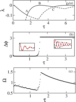
Figure 1: (Color online) (a) Lyapunov exponents of coupled harmonic oscillators Eq. (1) as a function of the time–delay $\tau$ for fixed $\epsilon$ = 1; (b) phase difference between the oscillators around point A indicated in (a). Inset figures show trajectories $x_{1}$ and $x_{2}$ as a function of time for the in–phase and the out–of–phase dynamics at $\tau$ =1 and 2 respectively, namely on either side of the phase–flip transition, and (c) the frequency of oscillation of the subsystems.

The uncoupled conservative Hamiltonian systems are made dissipative through the time–delay coupling, and this is also reflected in the fact that the sum of all the LEs remains negative for all $\tau$. Defining the energy of the individual oscillators as

$$E_{j}=(\dot{x}_{j}^{2}+\Omega_{j}^{2}x_{j}^{2})/2$$ (3)

where $\Omega_{j}$ is the instantaneous frequency of oscillation, the approach to the fixed point can be seen to be at an exponential rate in the AD regime trans as can be seen in Fig. 2(a). The exponential decay is however modulated, the oscillatory behavior being due to coupling (see the inset in the figure). In order to capture the dynamics, we define a decay constant as

$$e_{j} =\langle\,\ln|E^{m+1}_{j}-E^{m}_{j}|\rangle_{m}$$

$$\xi_{j} =\langle\,e_{j}\,\rangle_{IC}$$ (4)

where $E^{m}_{j}$ represents the $m$-th maxima in the energy time series of the $j$th oscillator. The averages $\langle\cdot\rangle_{m}$ and $\langle\cdot\rangle_{IC}$ are performed on $m$ and 100 initial conditions respectively.

Since the oscillatory behavior is modulated by exponential decay, $E^{m+1}_{j}-E^{m}_{j}$ is also an exponentially decaying function of $m$, at rate $\xi_{j}$. This rate can be measured experimentally and its variation with $\tau$ is shown in Fig. 2(b); the variation mirrors that of the frequency change at phase–flip, suggesting that energy decays more rapidly before the transition than after it.

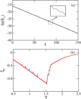
Figure 2: (Color online) (a)Energy of one of the oscillators, Eq. (3), as a function of time for $\tau=1$. The marked box is expanded in the inset. (b) The decay rate, $\xi_{1}$ as a function of $\tau$ (see Eq. (4)). Errorbars (marked in red) are calculated for 100 initial conditions.

At the critical delay values $\tau=n\pi/\omega$ (see points B and D in Fig. 1(a)) the largest Lyapunov exponent is zero and thus the motion is periodic. Fig. 3(a) shows orbits for five different initial conditions at the critical point; these resemble invariant curves as in conservative systems. However, in the vicinity of the critical delay values the largest lyapunov exponent is near zero and the motion appears periodic after an initial transient. The time series of one such periodic orbit is shown in Fig. 3(b). Also, as can be seen in the inset, there is very slow decrease in amplitude. This occurs since delay is not strictly $\tau_{c}$.

Away from delay $\tau_{c}$, the dissipation is more pronounced. The rate of decrease of the amplitude can be quantified through the measure

$$d_{j} =\langle\,|x_{j}^{m+1}-x_{j}^{m}|\,\rangle_{m}$$

$$\delta_{j} =\langle d_{j}\,\rangle_{IC}$$ (5)

where $x_{j}^{m}$ is the $m$-th maxima of $x_{j}$. This is plotted in Fig. 3(c) as a function of $\tau$ in the vicinity of $\tau=\pi/\omega$, namely the point B in Fig. 1(a). At $\tau=n\pi/\omega$ the rate of decrease of amplitudes approaches zero and hence the orbits are almost periodic. Similar behavior is observed at point D of Fig.1(a).

The reason for reappearance of oscillatory motion is straightforward. When the delay is a multiple of half the natural period of oscillation, then the coupling term effectively vanishes since

$$\dot{x}_{k}(t-\tau)\approx\dot{x}_{j}(t)$$ (6)

and the system effectively becomes conservative. Clearly when this occurs, each initial condition gives rise to an invariant curve (or, in this case, a nearly invariant curve). The better the equality above is realized, the more long lived the transients are.

There is the phase–flip transition at A, C and also higher values of $\tau$. At each transition a phase difference of $\pi$ is introduced between the oscillators resulting in anti–phase synchronization at $\tau=T/2$ and in–phase synchrony as $\tau=T$ and so on. Hence, the coupling function becomes zero at these critical delays. The consecutive oscillatory states alternate between having the oscillations being in–phase or out–of–phase, as shown in Fig. 3(d) (out–of–phase at $\tau=\pi/\omega$, namely at B) and Fig. 3(e) (in–phase at $\tau=2\pi/\omega$ at the point marked $D$) respectively. Note that the phase-relation between oscillators is independent of the initial conditions.

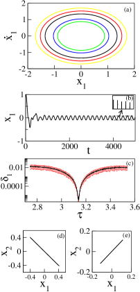
Figure 3: (Color online) (a) Periodic orbits with five different initial conditions at $\tau=\pi/\omega$; (b) time series of position variable $x_{1}$ as a function of time at $\tau=3.14$. The inset figure shows decrease in amplitude of $x_{1}$; (c) The averaged distance $\delta_{1}$ with errorbars, as function of delay $\tau$ near $\tau=\pi/\omega$. The errorbars are calculated for 100 initial conditions; (d) out-of-phase motion and (e) in-phase motion in relative phase plane $x_{1}-x_{2}$ at $\tau=\pi/\omega$ and $2\pi/\omega$ respectively (corresponding to points B and D of Fig. 1(a)).

III Coupled Hénon-Heiles systems

In order to examine the dynamics when the uncoupled systems are capable of exhibiting chaotic motion, we examine the behavior of two non-integrable Hénon-Heiles systems tabor ,

$$\ddot{x}_{j}+x_{j}+2x_{j}y_{j}-\epsilon(\dot{x}_{k}(\tau-t)-\dot{x}_{j}(t)) = 0$$

$$\ddot{y}_{j}+y_{j}+x_{j}^{2}-y_{j}^{2} = 0$$ (7)

As is well–known, in the uncoupled case ($\epsilon$=0) the system has both regular and irregular behavior largely depending on the total energy as well as on the initial condition tabor . Shown in Fig. 4 are the Poincaré maps for two different initial conditions, one leading to regular motion (red points), while another leads to chaotic dynamics (black points), at the same energy $E_{j}$ = 0.13 just below the dissociation limit $E_{j}$ = 1/6.

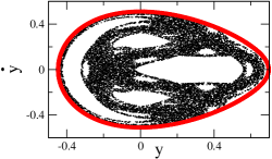
Figure 4: (Color online) (a) Poincaré map of two orbits in the Hénon-Heiles system, Eq. (7), at energy $E_{j}=0.13$. Red (outer) and black (inner) dots represent regular and chaotic motion respectively.

III.1 Instantaneous coupling $(\tau=0)$

In the absence of delay $\tau=0$, Eq. (7) reduces to the case of simple diffusive coupling. The effect of increasing the coupling strength, namely $\epsilon$, is to induce simplicity to the resulting collective dynamics. Shown in Fig.(5) are the the fraction of initial conditions $(f)$ leading to quasiperiodic motion. We take 100 pairs of random initial conditions from the bounded region of phase space (Fig. 4). In one case, when the initial condition pairs of quasiperiodic motions are taken, the collective dynamics due to interaction remains quasiperiodic (solid line (black circles): $QP+QP$). However, if the initial motion is chaotic then the resulting dynamics becomes quasiperiodic only after certain value of coupling strength (dashed line (red triangles): $C+C$). Similar behavior is observed when initial conditions of mixed chaotic and quasiperiodic motions are used (dotted line (green stars): $C+QP$). These results indicate that for small coupling strength the Hamiltonian structure still exists, but for larger values of coupling the collective dynamics becomes quasiperiodic; in this sense coupling induces simplicity in such coupled systems.

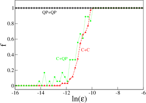
Figure 5: (Color online) Fraction of initial conditions that lead to quasiperiodic motion. The solid (black circles), dashed (red triangles) and dotted (green stars) curves are the results for the different cases of initial conditions corresponding to quasiperiodic ($QP+QP$), chaotic ($C+C$) and mixed chaotic and quasiperiodic $(C+QP)$ motions respectively. Averages have been taken over a sample of 100 initial conditions.

III.2 Time delay coupling

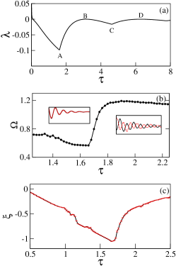
Figure 6: (Color online) (a) Largest Lyapunov exponent as a function of the time–delay, $\tau$, and (b) the oscillation frequency, for coupling strength $\epsilon$ = 1. The inset shows trajectories $x_{1}(t)$ and $x_{2}(t)$ for $\tau$ =1.4 and 1.8 respectively. (c) The decay constant $\xi_{1}$ as a function of the delay $\tau$.

When the two systems are coupled in presence of delay, $\tau$ (initial conditions taken from either the regular or irregular motion) the largest Lyapunov exponent quickly becomes negative. This is shown as a function of the delay in Fig. 6(a): almost as soon as the delay is switched on the oscillators are driven to AD state. The phenomenology of this higher dimensional system is very similar to that of the coupled harmonic oscillators: the largest LE has the same characteristic shape—there is a change in the slope at point A, where it is clear that the phase-flip transition occurs. Shown in Fig. 6(b) is the common frequency of oscillations as a function of delay which changes discontinuously at $\tau\sim$1.65. Since the phase of the oscillators is not clearly defined in such systems, we infer the phase relation from the time–series (inset figures) of the two systems in the neighborhood of the point of discontinuity. The phase difference changes from 0 to $\pi$ along with the frequency jump as in the simpler 1–dimensional harmonic system.

Here also energy decreases exponentially in this AD region. We define the energy of individual systems in the usual manner tabor

$$E_{j}=\frac{\dot{x_{j}}^{2}+\dot{y_{j}}^{2}}{2}+\frac{{x_{j}}^{2}+{y_{j}}^{2}}{2}+x_{j}^{2}y_{j}-\frac{y_{j}^{3}}{3},$$ (8)

and quantify the energy dissipation as in Eq. (3) by a quantifier $\xi_{j}$. The variation of this quantity with $\tau$ can be seen in Fig. 6(c). It confirms that energy dissipation is faster before phase flip transition and slower thereafter.

When the largest Lyapunov exponents approach zero (at points marked B and D in Fig. 6(a)) the motion is oscillatory, decaying very slowly to the fixed point. Critical delays are at half the natural time period of oscillation, and since the natural frequencies of the oscillators is equal to ‘1’, the time period is 2$\pi$. The Poincaré sections of representative trajectories at $\tau=3.14$ are shown in Fig. 7(a) which are quasiperiodic (cf. Section IIA). In the vicinity of this point, the rate of decay can be computed numerically as discussed earlier, and the quantifier $\delta$, Eq. (5) defined to locate the oscillatory state also has a minimum for at $\tau\approx 3.14$. At successive critical points ($\tau=3.14$ and $\tau=6.28$) the quasiperiodic motions alternate in the nature of the phase synchrony; see Fig. 7(d,e). Unlike the case of harmonic oscillators, though, the coupling term does not quite vanish, so the emergence of oscillations is not as pronounced in this case.

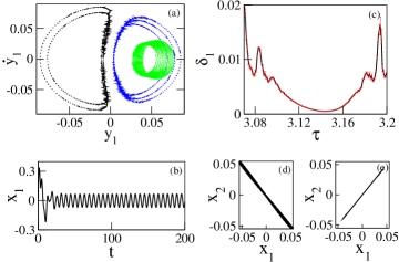
Figure 7: (Color online) (a) Poincaré section at $\tau=3.14$ for three different initial conditions; (b) time series of $x_{1}$; (c) variation of $\delta_{1}$ as a function of delay. The error bars are computed from a large number of initial conditions. (d) The relative phase in $x_{1}-x_{2}$ plane to show anti-phase motion at $\tau=\pi$ and (e) in-phase motion at $2\pi$.

IV Summary and Discussion

In the present paper we have explored the effects of incorporating time–delay in the coupling between Hamiltonian systems. The coupled system effectively becomes dissipative, and in the absence of other attractors, the total system displays amplitude death. However the coupling can effectively vanish for specific values of the time–delay, at which delay the the system naturally appears to be conservative. We find that this behaviour differs from that of delay–coupled non–Hamiltonian systems, where AD islands are separated by finite ranges of delay values where the coupling function need not vanish.

Orbits near these critical delay values reflect both dissipative and conservative behavior: different initial conditions give rise to different (seemingly) invariant curves which are very long lived transients. Energy dissipation in the AD regime is found to be associated with the phase–flip transition, and the damping is faster prior to the transition, and slower after it.

The finite velocity with which signals are transmitted gives rise to intrinsic delays in the coupling, and as such this is germane in both dissipative as well as conservative systems. Nevertheless, the effect of delay has been explored to a limited extent in conservative systems. The results presented here may have more general applicability in coupled systems with other conservation laws such as in ecological contexts eco .

Acknowledgment: GS gratefully acknowledges the support of the CSIR, India. AP and RR acknowledge the research support of the Department of Science and Technology (DST). AP also acknowledges DST for DU-DST-Purse grant for financial support. This work was started when AP was a sabbatical visitor at the MPI-PKS in Dresden, Germany, and he acknowledges their kind hospitality.

References

- (1) L. M. Pecora and T. L. Carroll, Phys. Rev. Lett. 64, 821 (1990); S. Pikovsky, M. G. Rosenblum, and J. Kurths, Synchronization: A Universal Concept in Nonlinear Sciences (Cambridge University Press, Cambridge, 2001).
- (2) Y. Yamaguchi and H. Shimizu, Physica 11D, 212 (1984);
- (3) K. Bar-Eli, Physica 14D, 242 (1985).
- (4) D. G. Aronson, , Physica 41D, 403 (1990); P. C. Mathews and S. H. Strogatz, Phys. Rev. Lett. 65, 1701 (1990); G. B. Ermentrout, Physica 41D, 219 (1990);
- (5) V. Resmi, G. Ambika and R. E. Amritkar, Phys. Rev. E 84, 046212 (2011); V. Resmi, G. Ambika, R. E. Amritkar and G. Rangarajan, Phys. Rev. E 85, 046211 (2012).
- (6) G. Saxena, A. Prasad, and R. Ramaswamy, Phys. Reports 521,205 (2012).
- (7) A. Prasad, Phys. Rev. E 72, 056204 (2005).
- (8) A. Prasad, J. Kurths, S. K. Dana and R. Ramaswamy, Phys. Rev. E 74, 035204 (2006); A. Prasad, S. K. Dana, R. Karnataka, J. Kurths, B. Blasius and R. Ramaswamy, Chaos 18, 23111, (2008); C. Masoller, M. Torrent and J. O. Garcia, Phil. Trans. R. Soc. A. 367, 3255 (2009); Y. Chen, J. Xiao, W. Liu, L. Li and Y. Yang, Phys. Rev. E 80, 046206 (2009); J. M. Cruz, J. Escalona, P. Parmananda, R. Karnatak, A. Prasad, and R. Ramaswamy, Phys. Rev. E. 81, 046213 (2010); B. M. Adhikari, A. Prasad, M. Dhamala, Chaos 21, 023116 (2011);
- (9) R. Karnatak, P. Nirmal, A. Prasad and R. Ramaswamy, Phys. Rev. E. 82, 046219 (2010); P. Nirmal, R. Karnatak, A. Prasad, J. Kurths and R. Ramaswamy, Phys. Rev. E 85, 046204 (2012).
- (10) S. Kim, S. H. Park and C. S. Ryu, Phys. Rev. Lett. 79, 2911 (1997); A. Prasad, L. D. Iasemidid, S. Sabesan and K. Tsakalis, Pramana 64, 513 (2005).
- (11) J. C. Sommerer and E. Ott, Nature 365, 138 (1993).
- (12) K. Kaneko, Theory and Applications of Coupled Map Lattices (John Wiley and Sons, New York, 1993).
- (13) H. G. Schuster and P. Wagner, Prog. Theo. Phys. 81, 939 (1989).
- (14) K. Konishi, M. Ishii and H. Kokame, Phys. Rev. E 54, 3455 (1996); K. Konishi, H. Kokame and K. Hirato, Phys. Rev. E 62, 384 (2000); K. Konishi, Phys. Rev. E 67, 017201 (2003); K. Konishi, K. Senda and H. Kokame, Phys. Rev. E 78, 056216 (2008); K. Konishi, H. Kokame and N. Hara, Phys. Rev. E 81, 016201 (2010); L. B. Le, K. Konishi and N. Hara, Nonlinear Dyn. 67, 1407,(2012).
- (15) D. V. Ramana Reddy, , Phys. Rev. Lett. 80, 5109 (1998); S. H. Strogatz, Nature (London) 394, 316 (1998); F. M. Atay, Phys. Rev. Lett. 91, 094101 (2003); F. M. Atay, J. Jost, Phys. Rev. Lett. 92, 144101 (2004); F. M. Atay, Physica 183D, 1 (2003); G. Saxena, A. Prasad, and R.Ramaswamy, Phys. Rev. E. 82, 017201 (2010).
- (16) W. Zou, C. Yao and M. Zhan, Phys. Rev. E 82, 056203 (2010); W. Zou, J. Lu, Y. Tang, C. Zhang and J. Kurths, Phys. Rev. E 84, 066208 (2011); W. Zou, Y. Tang, L. Li and J. Kurths, Phys. Rev. E 85, 046206 (2012); W. Zou, D. V. Senthilkumar, Y. Tang and J. Kurths, Phys. Rev. E 86, 036210 (2012).
- (17) V. Ravichandran, V. Chinnathambi and S. Rajshekar, Pramana 78, 2911 (2012).
- (18) M. Lakshamanan and D. V. Senthilkumar, Dynamics of Nonlinear Timedelay systems (Springer, India, 2011).
- (19) J. D. Farmer, Physica 4D, 366 (1982).
- (20) M. Tabor, Chaos and Integrability in Nonlinear Dynamics: An Introduction (John Wiley & Sons, New York, 1989).
- (21) V. I. Arnold, Mathematical Methods of Classical Mechanics (Springer, New York, 1978).
- (22) D. H. Zanette and A. S. Mikhailov, Phys. Lett. 235A, 135 (1997); A. Hampton and D. H. Zanette, Phys. Rev. Lett. 83, 2197 (1999).
- (23) Z. Wang and H. Hu, Proceedings of International Design Engineering Technical Conferences & Computers and Information in Engineering Conference (2005).
- (24) Similar results are found for mismatched oscillators.
- (25) The flow is integrated using the Runge-Kutta order scheme with integration step where is fixed. As we increase the value (checked upto ) the decrease in amplitude in Fig. 3(b) becomes slower. Lyapunov exponents are calculated using the method as given in Ref. farmer .
- (26) Phase and frequency are numerically calculated as per Ref. pf .
- (27) Understanding the transient dynamics is essential in describing AD since this state is asymptotically featureless. Transients can be significant in applications that are restricted to finite times, as for example in ecology tra .
- (28) A. Hatings, Eco. Lett. 215, 4 (2001); O. Ovaskainen, I. Hanski Theor. Popul. Biol. 61, 285 (2002);
- (29) Y. Nutku, Phys. Lett. 145A, 27 (1990).