TILTED SEXTUPOLES FOR CORRECTION OF CHROMATIC ABERRATIONS IN BEAM LINES WITH HORIZONTAL AND VERTICAL DISPERSIONS

Abstract

In this article we discuss the usage of tilted multipoles for correction of chromatic aberrations in the design of the beam switchyard arc at the European X-Ray Free-Electron Laser (XFEL) Facility [2].

1 INTRODUCTION

The European XFEL has been planed as a multiuser facility and from the beginning will have the possibility to distribute electron bunches of one beam pulse to one or the other of two electron beamlines, each serving its own set of undulators. Additional space is reserved for the later addition of a third electron beamline. Because different users have contradictory requirements to the bunch repetition pattern, operational flexibility will be reached by a distribution system which will use very stable flat-top kickers for directing beam into the undulator beamlines and fast single bunch kickers to kick individual bunches into the transport line to the beam dump before the beam distribution [2, 3].

Both, the beam separation between undulator beamlines and beam deflection into the beam dump will be realized with a kicker-septum scheme. While the beam quality in the dump line is not an issue, the optics of the beam separation between two undulator beamlines must meet a very tight set of performance specifications. It should be able to accept bunches with different energies (up to $\pm 1.5\%$ from nominal energy) and transport them without any noticeable deterioration not only transverse, but also longitudinal beam parameters, i.e. it must be sufficiently achromatic and sufficiently isochronous. Besides that it is necessary to avoid magnet collisions in the design, and to keep the degradation of the beam quality due to collective effects within acceptable limits.

In this paper we discuss the optics solution for the beam separation area between two undulator beamlines (see Fig.1) with the main attention played to the improvement of the chromatic properties of the beam deflection arc by usage of sextupole and octupole magnets. Because of the Lambertson type septums used in the design, the deflection arc has nonzero horizontal and vertical dispersions simultaneously. This means that regardless of the fact that the linear on-energy betatron motion is still transversely uncoupled in such a beamline, we have not only the non-linear dispersions generated in both transverse planes, but also vertical and horizontal oscillations become chromatically coupled due to vertical dispersion in the horizontal bending magnets and horizontal dispersion in the vertical dipoles. Nevertheless, because these effects are not the result of magnet misalignments and imperfections and are well controlled by the linear optics design, the usage of tilted sextupoles and octupoles in such a beamline allows to maintain the total number of multipoles required for correction of chromatic aberrations on the same level as required in the mid-plane symmetric systems.

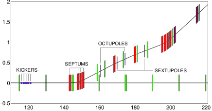
Figure 1: Top view of the separation area between two electron beamlines. Green, red and purple colors mark quadrupole magnets, and horizontal and vertical dipole magnets, respectively. Horizontal and vertical distances are measured in meters.

2 SECOND-ORDER CHROMATIC ABERRATIONS DUE TO SEXTUPOLES

In this section we give formulas for the sextupole contributions to the second-order chromatic aberrations from which one can see similarities and differences in the usage of tilted sextupole magnets in the beamlines with non-flat dispersion and in beamlines which bend the beam only horizontally (formulas (7)-(21) with arbitrary angle $\theta$ and with angle $\theta$ multiple of $180^{\circ}$, respectively). The effect of octupoles can be calculated and analyzed in a similar fashion and due to space limitation is not given here.

As usual, we take the path length along the reference orbit $\tau$ to be the independent variable and use a complete set of symplectic variables $\mbox{\boldmath$z$}=(x,p_{x},y,p_{y},\sigma,\varepsilon)$ as particle coordinates [4, 5]. In these variables the Hamiltonian describing the motion of a particle in the magnetostatic system of interest can be written as

$$H(\mbox{\boldmath$z$})\,=\,\varepsilon-(1+hx+\alpha y)\cdot\Big{[}\Big{(}(1+\varepsilon)^{2}\Big{.}\Big{.}$$

$$\Big{.}\Big{.}-(p_{x}-\bar{A}_{x})^{2}-(p_{y}-\bar{A}_{y})^{2}-(\varepsilon/\gamma_{0})^{2}\Big{)}^{1/2}+\bar{A}_{z}\Big{]},$$ (1)

where $\bar{A}_{x}$, $\bar{A}_{y}$ and $\bar{A}_{z}$ are the components of the magnetic vector potential multiplied by the rigidity of the reference particle, and $h$ and $\alpha$ are the horizontal and vertical curvatures of the reference orbit, respectively. We assume that $h(\tau)\cdot\alpha(\tau)\equiv 0$ and that both curvatures are positive if the reference orbit bends in the direction opposite to that of the corresponding coordinate axis. With the assumption that all magnets in our system are multipoles of separate function type and with appropriately chosen vector potential, the Hamiltonian (1) expanded up to third order in the variables $z$ then takes the form $H=_{3}H_{2}+H_{3}$, where

$$H_{2}\,=\,(1\,/\,2)\,\big{(}p_{x}^{2}+p_{y}^{2}+\varepsilon^{2}\,/\,\gamma_{0}^{2}\big{)}\,-\,(hx+\alpha y)\,\varepsilon$$

$$+\,(1\,/\,2)\,\big{(}h^{2}+k_{1}\big{)}\,x^{2}\,+\,(1\,/\,2)\,\big{(}\alpha^{2}-k_{1}\big{)}\,y^{2},$$ (2)

$$H_{3}=(1\,/\,2)\,\big{(}hx+\alpha y-\varepsilon\big{)}\,\big{(}p_{x}^{2}+p_{y}^{2}+\varepsilon^{2}\,/\,\gamma_{0}^{2}\big{)}$$

$$-\,(1\,/\,2)\,\big{(}h^{\prime}p_{x}-\alpha^{\prime}p_{y}\big{)}\,\big{(}x^{2}-y^{2}\big{)}$$

$$-\,(1\,/\,6)\big{(}h^{\prime\prime}\,x^{3}+\alpha^{\prime\prime}\,y^{3}\big{)}\,+\,k_{2}\,V_{s},$$ (3)

$$V_{s}\,=\,\cos(3\varphi)\,\frac{x^{3}-3xy^{2}}{6}\,-\,\sin(3\varphi)\,\frac{y^{3}-3x^{2}y}{6},$$ (4)

and $=_{n}$ means equality up to order $n$, prime denotes differentiation with respect to the variable $\tau$, $\varphi$ is a sextupole tilt angle, and $k_{1}$ and $k_{2}$ are quadrupole and sextupole coefficients, respectively.

We represent particle passage through our system by a symplectic map $\,{\cal M}\,$ that maps the dynamical variables  $z$  from the location $\tau=0$ to the location $\tau=l$ and use for this map the following Lie factorization

$$:{\cal M}:\,=_{2}\,\exp(:{\cal F}_{3}(\mbox{\boldmath$z$}):)\,:M(l):.$$ (5)

Here $M(\tau)=(r_{km}(\tau))$ is a fundamental matrix solution of the linearized system driven by the Hamiltonian (2) and the function ${\cal F}_{3}$ is a third order homogeneous polynomial:

$${\cal F}_{3}(\mbox{\boldmath$z$})\,=\,-\int_{0}^{l}H_{3}(\tau,\,M(\tau)\cdot\mbox{\boldmath$z$})\,d\tau.$$ (6)

We separate the polynomial ${\cal F}_{3}$ in two parts ${\cal F}_{3}={\cal F}_{3}^{o}+{\cal F}_{3}^{s}$, where ${\cal F}_{3}^{s}$ describes the sextupole effects, and use a notation $c_{abcde}({\cal F}_{3}^{s})$ for the coefficient with which the monomial $\,x^{a}\,p_{x}^{b}\,y^{c}\,p_{y}^{d}\,\varepsilon^{e}\,$ enters the polynomial ${\cal F}_{3}^{s}$. Using polar coordinates $r_{D}$ and $\theta$ for the $r_{16}$ and $r_{36}$ elements, namely taking $r_{16}=r_{D}\cos(\theta)$ and $r_{36}=r_{D}\sin(\theta)$, the formulas for the sextupole contributions to the chromatic aberrations can be written as follows.

Chromatic Coupling Terms

$$c_{10101}({\cal F}_{3}^{s})\,=\,\int_{0}^{l}k_{2}\,r_{11}\,r_{33}\,r_{D}\,\sin(\theta-3\varphi)\,d\tau,$$ (7)

$$c_{01011}({\cal F}_{3}^{s})\,=\,\int_{0}^{l}k_{2}\,r_{12}\,r_{34}\,r_{D}\,\sin(\theta-3\varphi)\,d\tau,$$ (8)

$$c_{10011}({\cal F}_{3}^{s})\,=\,\int_{0}^{l}k_{2}\,r_{11}\,r_{34}\,r_{D}\,\sin(\theta-3\varphi)\,d\tau,$$ (9)

$$c_{01101}({\cal F}_{3}^{s})\,=\,\int_{0}^{l}k_{2}\,r_{12}\,r_{33}\,r_{D}\,\sin(\theta-3\varphi)\,d\tau.$$ (10)

Chromatic Focusing Terms

$$c_{20001}({\cal F}_{3}^{s})\,=\,-\frac{1}{2}\int_{0}^{l}k_{2}\,r_{11}^{2}\,r_{D}\,\cos(\theta-3\varphi)\,d\tau,$$ (11)

$$c_{02001}({\cal F}_{3}^{s})\,=\,-\frac{1}{2}\int_{0}^{l}k_{2}\,r_{12}^{2}\,r_{D}\,\cos(\theta-3\varphi)\,d\tau,$$ (12)

$$c_{11001}({\cal F}_{3}^{s})\,=\,-\int_{0}^{l}k_{2}\,r_{11}\,r_{12}\,r_{D}\,\cos(\theta-3\varphi)\,d\tau,$$ (13)

$$c_{00201}({\cal F}_{3}^{s})\,=\,\frac{1}{2}\int_{0}^{l}k_{2}\,r_{33}^{2}\,r_{D}\,\cos(\theta-3\varphi)\,d\tau,$$ (14)

$$c_{00021}({\cal F}_{3}^{s})\,=\,\frac{1}{2}\int_{0}^{l}k_{2}\,r_{34}^{2}\,r_{D}\,\cos(\theta-3\varphi)\,d\tau,$$ (15)

$$c_{00111}({\cal F}_{3}^{s})\,=\,\int_{0}^{l}k_{2}\,r_{33}\,r_{34}\,r_{D}\,\cos(\theta-3\varphi)\,d\tau.$$ (16)

Terms Responsible for the Second Order
Transverse and Longitudinal Dispersions

$$c_{10002}({\cal F}_{3}^{s})\,=\,-\frac{1}{2}\int_{0}^{l}k_{2}\,r_{11}\,r_{D}^{2}\,\cos(2\theta-3\varphi)\,d\tau,$$ (17)

$$c_{01002}({\cal F}_{3}^{s})\,=\,-\frac{1}{2}\int_{0}^{l}k_{2}\,r_{12}\,r_{D}^{2}\,\cos(2\theta-3\varphi)\,d\tau,$$ (18)

$$c_{00102}({\cal F}_{3}^{s})\,=\,\frac{1}{2}\int_{0}^{l}k_{2}\,r_{33}\,r_{D}^{2}\,\sin(2\theta-3\varphi)\,d\tau,$$ (19)

$$c_{00012}({\cal F}_{3}^{s})\,=\,\frac{1}{2}\int_{0}^{l}k_{2}\,r_{34}\,r_{D}^{2}\,\sin(2\theta-3\varphi)\,d\tau.$$ (20)

$$c_{00003}({\cal F}_{3}^{s})\,=\,-\frac{1}{6}\int_{0}^{l}k_{2}\,r_{D}^{3}\,\cos(3\theta-3\varphi)\,d\tau.$$ (21)

3 BEAM DEFLECTION ARC

The beam deflection arc starts from the kickers which deflect beam vertically and, after enhancement of this deflection by the following quadrupole, the beam arrives at the entrance of the first Lambertson septum magnet with the vertical separation from the horizontal midplane $y=0$ of about $18\,mm$. The first septum magnet is tilted by approximately $11^{\circ}$ in such a way that it bends particles not only horizontally but also slightly upward. It is done in order to compensate the downward deflection produced by the vertically focusing large aperture quadrupole that follows after the septum, and in order to have the beam traveling in parallel to the horizontal midplane at the entrance of the three remaining (non-tilted) septum magnets, as can be seen in Fig.1 and Fig.2. The rest of the deflection arc is constructed from ordinary multipoles and the arc ends by a dogleg consisting of two vertical dipoles, which is used for bringing beam back to the horizontal plane $y=0$ and for closing the linear vertical dispersion. The $r_{56}$ coefficient of the transfer matrix of the total deflection arc (considered from the entrance of the first kicker up to the exit of the last vertical dipole) is equal to zero, i.e. the deflection arc is a first-order isochronous beamline. This is achieved by usage of two reverse bend dipoles placed close to the arc center. The entrance Twiss parameters of the deflection arc are fixed and are defined by the behavior of the betatron functions in the straight beamline. The exit Twiss functions are such that they allow easy matching to the periodic downstream transport channel (see Fig.3). Two tilted sextupoles and two tilted octupoles are placed in the arc to provide the required chromatic properties of the beam transport (see Fig.1 and Fig.4). Note that the optimization of the number of sextupoles and octupoles, and their positions, strengths and tilt angles was not a separate task after the finishing of

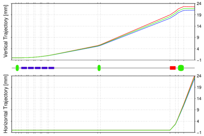
Figure 2: Trajectories of the kicked particles in the beginning of the separation area. The relative energy deviations are equal to $-3\%,\,0\%$ and $+3\%$ (red, green and blue curves, respectively).

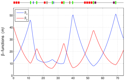
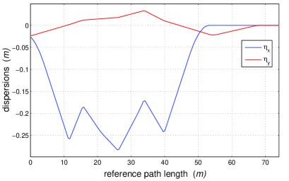
Figure 3: Betatron and dispersion functions along deflection arc shown starting from the entrance of the first non-tilted septum.

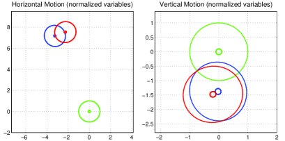
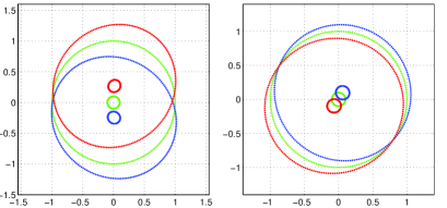
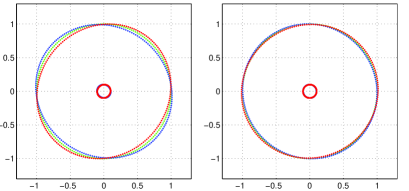
Figure 4: Phase space portraits of monochromatic $0.1\sigma_{x,y}$ and $1\sigma_{x,y}$ ellipses (matched at the entrance) after tracking through the deflection arc. The relative energy deviations are equal to $-1.5\%,\,0\%$ and $+1.5\%$ (red, green and blue ellipses, respectively). Sextupoles and octupoles are switched off (upper plots), sextupoles are on and octupoles are off (middle plots), sextupoles and octupoles are on (lower plots).

the design of the linear optics, but both, linear and non-linear optics were designed together.

The arc design presented in this paper meets all design specifications from the point of view of single particle beam dynamics. The impact of collective effects on the beam quality still requires additional investigations [6].

References

[1]
[2] M.Altarelli, R.Brinkmann et al. (Eds),
“XFEL: The European X-Ray Free-Electron Laser. Technical Design Report”,
DESY 2006-097, DESY, Hamburg, 2006.
[3] W.Decking, F.Obier,
“Layout of the Beam Switchyard at the European XFEL”,
EPAC08-WEPC073, Genoa, Italy, 2008.
[4] H.Mais and G.Ripken,
“Theory of Coupled Synchro-Betatron Oscillations (I)”,
Internal Report, DESY M-82-05, 1982.
[5] V.Balandin and N.Golubeva,
“Hamiltonian Methods for the Study of Polarized Proton Beam Dynamics
in Accelerators and Storage Rings”,
DESY 98-016, February 1998.
[6] M.Dohlus,
“Impact of CSR Effects in the XFEL Collimation Section and Beam Distribution”,
FEL Beam Dynamics Group Meeting, 29.06.2009,
http://www.desy.de/xfel-beam/talks.html