Multi-Scale Codes in the Nervous System:
The Problem of Noise Correlations
and the Ambiguity of Periodic Scales

Abstract

Encoding information about continuous variables using noisy computational units is a challenge; nonetheless, asymptotic theory shows that combining multiple periodic scales for coding can be highly precise despite the corrupting influence of noise Mathis et al. (2012a). Indeed, cortex seems to use such stochastic multi-scale periodic ‘grid codes’ to represent position accurately. We show here how these codes can be read out without taking the asymptotic limit; even on short time scales, the precision of neuronal grid codes scales exponentially in the number $N$ of neurons. Does this finding also hold for neurons that are not statistically independent? To assess the extent to which biological grid codes are subject to statistical dependencies, we analyze the noise correlations between pairs of grid code neurons in behaving rodents. We find that if the grids of the two neurons align and have the same length scale, the noise correlations between the neurons can reach $0.8$. For increasing mismatches between the grids of the two neurons, the noise correlations fall rapidly. Incorporating such correlations into a population coding model reveals that the correlations lessen the resolution, but the exponential scaling of resolution with $N$ is unaffected.

I Introduction

Multi-scale basis functions, such as simple Fourier transforms or wavelets, have a long history, dating back to the 19th century. They are widely used for data compression, processing and analysis Haar (1909); Chui (1992); Unser and Aldroubi (1996); Mallat (2009). For instance, state-of-the-art image compression algorithms convolve images with a discrete cosine or Haar transform at different length scales Acharaya and Tsai (2005) . Wavelets at multiple scales or “steerable pyramids” Simoncelli et al. (1992); Riesenhuber and Poggio (1999) are used both in machine and biological vision. Indeed, the receptive fields observed in the early visual system Hubel and Wiesel (1968); DeValois and DeValois (1990) resemble wavelets; moreover, they emerge naturally in optimally sparse codes for the visual and auditory systems of mammals Olshausen and Field (1996); Lewicki (2002).

In the last decade, neuroscientists working in the medial entorhinal cortex (mEC), pre- and parasubiculum have discovered periodic neuronal tuning curves Hafting et al. (2005); Boccara et al. (2010) for stimuli that are not intrinsically periodic. Neurons with such tuning curves fire spikes at regularly spaced locations within an environment. The resulting map of spatial firing resembles a hexagonal grid, inspiring the researchers to call these neurons ‘grid cells’. The grids within the same cortical area have a finite number of different length scales and the ratio of one length scale to the next shorter seems to be constant  Barry et al. (2007); Stensola et al. (2012), in accordance with optimal coding theory Mathis et al. (2012b, a); Wei et al. (2013).

What role do periodic tuning curves and multiple scales play in coding? Recently, we computed the Fisher information for population codes with such properties and showed that their precision can scale exponentially in the number of neurons Mathis et al. (2012b, a), as long as the neurons fired independently. In contrast, the precision of population codes with unimodal or sigmoidal tuning curves scale linearly in the number of neurons Seung and Sompolinsky (1993); Zhang and Sejnowski (1999); Wilke and Eurich (2001); Bethge et al. (2002); Brown and Bäcker (2006); McDonnell and Stocks (2008); Nikitin et al. (2009). In this paper, we address two major concerns that might affect the feasibility of multi-scale codes:

• Tuning curves with multiple peaks compound the ambiguity already inherent in a stochastic representation; this ambiguity can lead to catastrophic decoding errors. As the Fisher information is a local, asymptotic measure of coding accuracy, we had provided quantitative bounds for the probability of catastrophic errors. Here we show how the probability of a stimulus $x$ given the population response can be calculated analytically. This allows us to estimate the true coding error, even for high-dimensional stimuli and population responses that are sampled only for short time periods.

• Neurons from the same area in cortex at times display correlated fluctuations that are unrelated to the stimulus being encoded. Such noise correlations can be detrimental to the encoding accuracy of population codes Zohary et al. (1994); Schneidman et al. (2006); Ecker et al. (2010); Cohen and Kohn (2011). Much of the experimental Zohary et al. (1994); Lee et al. (1998); Smith and Kohn (2008); Ecker et al. (2010); Cohen and Kohn (2011); Miura et al. (2012) and theoretical work Abbott and Dayan (1999); Shamir and Sompolinsky (2001); Wilke and Eurich (2001); Shamir and Sompolinsky (2006); Ecker et al. (2011) has focused on sensory and motor areas of the brain. In contrast, brain regions, such as the hippocampus and medial entorhinal cortex (mEC) are less well studied in this context. As these areas form a central hub of computation, receiving and sending information from many other brain areas, correlated fluctuations might be a byproduct of the neuronal network’s processing. Here we quantify the noise correlations of grid cells in the entorhinal cortex (EC) of behaving rodents and study their effect on the coding accuracy.

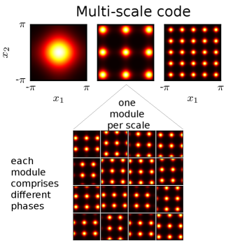
Figure 1: Illustration of a multi-scale code. The population consists of neurons that encode the stimulus with tuning curves $\Omega_{i}(x)$ that vary in scale and whose amplitude is shown in color. Each scale comprises a group of cells with periodic tuning curves on an identical lattice structure but different shifts (phases) – an arrangement we call a module. Such a population of nested modules successively refines the representation of the stimulus. For a single module, the mapping from stimulus to periodic population response is not injective; only the response over the whole ensemble of modules provides a unique representation of the stimulus within $[-\pi,\pi)^{2}$.

The paper is organized as follows. First, we compute the maximum likelihood estimate of the stimulus from the neuronal response, and compare the resulting error to the prediction from the Fisher information. Second, we analyze the effect of noise correlations on the Fisher information in multi-scale population codes and compare these results to numerical estimates of the mean square error (MSE). Third, we analyze the noise correlations between grid cells from real data (provided by the Moser lab at the Norwegian University of Science and Technology Hafting et al. (2008)) to corroborate the correlated noise model we used. We find that although noise correlations reduce the overall accuracy, multi-scale codes, as found in mEC, are still vastly superior to single-scale codes.

II The Precision of Multi-scale Codes—Long-Term Asymptotics versus Short-Term Estimates

Take a population of $N$ neurons. In response to a stimulus $\bm{x}\in I\subset\mathds{R}^{D}$, the activity of the $i$-th neuron is

$$\Upsilon_{i}(\bm{x})=\Omega_{i}(\bm{x})+\eta_{i}(\bm{x}).$$ (1)

Here $\Omega_{i}(\bm{x})$ is the average response of neuron $i$, also known as the neuron’s tuning curve, while $\eta_{i}$ represents the trial-to-trial variability. The variability $\eta_{i}(\bm{x})$ has zero mean by definihtion, but may be correlated across neurons— a case that we treat in the next section.

In previous work Mathis et al. (2012a, b), we argued that a population code should consist of periodic, multi-scale tuning curves $\Omega_{i}(\bm{x})$, as exemplified by the von Mises functions in one dimension:

$$\Omega_{i}(x)=f_{max}\tau\cdot\exp\left(\frac{\cos(2\pi/\lambda_{i}(x-\varphi_{i}))-1}{\sigma^{2}}\right),$$ (2)

as illustrated in Fig. 1. The tuning curve $\Omega_{i}(\bm{x})$ of each cell $i$ is characterized by a scale $\lambda_{i}$, a preferred phase $\varphi_{i}$ and tuning width $\sigma$. The term $f_{max}$ denotes the peak firing rate (number of action potentials per unit time), which is assumed to be the identical for all neurons, and $\tau$ describes the characteristic time interval over which spikes are counted. These tuning curves would ideally be organized into different, nested modules such that all neurons within one module share the period $\lambda_{i}$ but exhibit different preferred phases $\varphi_{i}$. Such multi-scale population codes achieve exponentially higher precision in representing $x$ than unimodal codes, provided that the $\lambda_{i}$’s are arranged into a discrete, geometric progression Mathis et al. (2012b). Recent experimental results on grid codes in entorhinal cortex bear out this theoretical prediction Barry et al. (2007); Stensola et al. (2012).

Given a stimulus $x$, the response has a probability distribution $P({\bm{\Upsilon}}|\bm{x})$, where $\bm{\Upsilon}=(\Upsilon_{1},\dots,\Upsilon_{N})$ denotes the population’s response. The task for an ideal observer is to estimate $x$ from $\bm{\Upsilon}$ as $\hat{\bm{x}}$, for instance by choosing the most likely stimulus, or the one that minimizes ${\left\langle(\bm{x}-\hat{\bm{x}})^{2}\right\rangle}_{p(\bm{x})}$. Asymptotically, as ${f_{max}\tau}\to\infty$, a statistically efficient estimator $\hat{\bm{x}}$ will have a probability distribution that approaches

$$p(\hat{\bm{x}}-\bm{x})\sim\exp\left[-\frac{1}{2}{\left(\hat{\bm{x}}-\bm{x}\right)}^{T}{\mathbf{J}}\left(\hat{\bm{x}}-\bm{x}\right)\right],$$ (3)

at least as long as $\hat{\bm{x}}$ is close to the true $\bm{x}$. Here $\mathbf{J}$ is the Fisher information matrix at position $x$ with entries

$$\bm{J}_{{\alpha\beta}}(\bm{x})=\left\langle\left(\frac{\partial\ln P(\bm{\Upsilon}|\bm{x})}{\partial x_{\alpha}}\right)\left(\frac{\partial\ln P(\bm{\Upsilon}|\bm{x})}{\partial x_{\beta}}\right)\right\rangle_{P(\bm{\Upsilon}|\bm{x})},$$ (4)

where $\alpha$, $\beta\in\{1,\cdots,D\}$. Indeed, the Cramér-Rao bound strictly limits the error of any unbiased estimate of $x$ through the Fisher information

$$\left\langle(\bm{x}-\hat{\bm{x}})^{2}\right\rangle\geq\bm{J}(\bm{x})^{-1}.$$ (5)

The key question is: how close will an efficient estimator come to the Cramér-Rao bound? In a multi-scale, periodic grid code, $p\left(\bm{x}-\hat{\bm{x}}\right)$ will deviate from the Laplace approximation inherent in Eq. (3); the periodicity causes the distribution $p\left(\bm{x}-\bm{\hat{}}{\bm{x}}\right)$ to have multiple peaks. We now show how one can avoid the assumption of the asymptotic limit entirely, by extending a result of Yaeli and Meir Yaeli and Meir (2010) on Gaussian tuning curves.

For simplicity, let us start with one module of $M$ neurons, each with a tuning curve $\Omega_{i}(x)$ given by Eq. (2) on the one-dimensional interval $I=[-\pi,\pi)$. These tuning curves have a uniform period $\lambda_{0}=2\pi$ and tuning width $\sigma^{2}$, but the parameter $\varphi_{i}$ is distributed across different neurons, so that the tuning curves cover the interval uniformly. The prior probability of $p(x)$ is assumed to be uniform, and each neuron’s response $\Upsilon_{i}$ obeys a discrete Poisson distribution. If the neurons are statistically independent, then by Bayes’ rule

$$p\left(x|{\bm{\Upsilon}}\right)\sim \prod_{j=1}^{M}\text{Poisson}\left(\Upsilon_{j},\Omega_{j}(x)\right)$$

$$= \frac{\prod_{j=1}^{M}\exp(\Upsilon_{j}\ln\left(\Omega_{j}(x)\right)}{\prod_{j=1}^{M}\Upsilon_{j}!}\exp\!\!\left(\!\!-\sum_{j=1}^{M}\Omega_{j}(x)\!\!\right)$$

As observed by several authors Dayan and Abbott (2001); Yaeli and Meir (2010), if the tuning curves uniformly cover the interval, $$\sum_{j=1}^{M}\Omega_{j}(x)\approx\text{constant} M$$, even for relatively small . With this one approximation,

$$P\left(x|{\bm{\Upsilon}}\right)= C\cdot\exp\left(\kappa\sum_{j=1}^{M}\Upsilon_{j}\cos(x-\varphi_{j})\right),$$ (6)

where $$C \kappa=\sigma^{-2} \hat{\mu} \hat{\kappa}$$ is a normalization constant, and . We can express this posterior probability as a von Mises function with mean and concentration

$$P(x|\bm{\Upsilon})= C\exp\left\{\hat{\kappa}\cos\left[(x-\hat{\mu})\right]\right\}.$$ (7)

Within the interval $[-\pi,\pi)$, $x=\hat{\mu}$ corresponds to the peak of Eq. (6), so that $\hat{\mu}$ represents the most likely stimulus, given the neurons’ response. The concentration $\hat{\kappa}$ expresses the certainty about $\hat{\mu}$. We obtain

$$\hat{\mu}= \text{arg}\left(\sum_{j=1}^{M}\Upsilon_{j}\exp(i\,\varphi_{j})\right)$$

and

$$\hat{\kappa}= \kappa\sum_{j=1}^{M}\Upsilon_{j}\cos\left[\left(\hat{\mu}-\varphi_{j}\right)\right].$$

So the expected phase $\hat{\mu}\in[-\pi,\pi)$ is the response-weighted sum of the neurons’ preferred phases, also known as the population vector Georgopoulos, Schwartz  and Kettner (2001); Seung and Sompolinsky (1993). Both $\hat{\kappa}$ and $\hat{\mu}$ are random variables, as the population’s response vector $\bm{\Upsilon}$ is stochastic (see Fig. 2).

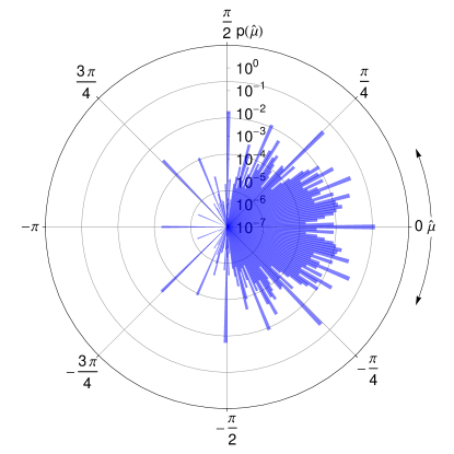
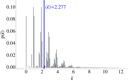
Figure 2: Distribution of estimates $\hat{\mu}$ and $\hat{\kappa}$: As the population response $\bm{\Upsilon}$ is stochastic, the posterior distribution $P(x|\bm{\Upsilon})$ depends on the random variables $\hat{\mu}$ and $\hat{\kappa}$, which govern the von Mises distribution in Eq. (7). The probability distributions of these two random variables are shown above for a single-scale module of neurons with $f_{\text{max}}\tau=1$, $M=16$, $\lambda_{0}=2\pi$ and $\sigma^{2}=1/7$. The quantity $\hat{\mu}$ is the maximum a posteriori (MAP) estimate of $x$. The asymptotic Fisher information $J$ is proportional to the expected value of $\hat{\kappa}$. For a given realization of $\bm{\Upsilon}$, the expected error can be greater or less than predicted by the asymptotic Cramér-Rao bound, depending on whether $\hat{\kappa}$ is less or greater than $\left\langle\hat{\kappa}\right\rangle$. If $\hat{\kappa}\gg 1$, then the expected error is $1/\hat{\kappa}$, and the Cramér-Rao bound for the average error is a consequence of Jensen’s inequality, $\left\langle 1/\hat{\kappa}\right\rangle\geq 1/\left\langle\hat{\kappa}\right\rangle=1/J$.

The expected value of $\hat{\kappa}$ is

$$\left\langle\hat{\kappa}\right\rangle=\kappa\int_{-\pi}^{\pi}\Omega(\hat{\mu}-\varphi)\cos\left(\hat{\mu}-\varphi\right)\,\rho(\varphi)d\varphi.\\$$

where $\rho(\varphi)$ represents the density of preferred phases of the tuning curves. With $M$ equidistantly spaced tuning curves along one dimension (with $x$ a scalar), we get $\left\langle\hat{\kappa}\right\rangle=\left(2\pi f_{max}\tau M\right)\kappa\exp(-\kappa)I_{1}(\kappa)$, where $I_{1}$ is the modified Bessel function of the first kind. This relates the expected concentration $\hat{\kappa}$ of the posterior probability to the inverse tuning width $\kappa=\sigma^{-2}$ of the tuning curves. Figure 2 emphasizes the fact that the variance of $\hat{\kappa}$ is large; indeed, this is always the case, as the $\text{variance}\!\left(\hat{\kappa}\right)\sim\kappa\langle\hat{\kappa}\rangle$ .

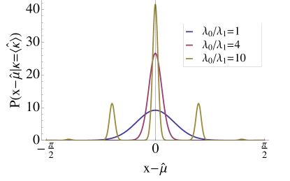
(a)

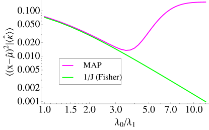
(b)

Figure 3: The typical error in estimating $x$ as the most likely stimulus given the neuronal response in a two-scale population code. To estimate this error, we replace $\hat{\kappa}_{i}$ and $\hat{\mu}_{i}$ in Eq. (10) by their expected values. Without loss of generality, we consider $x=0$. The parameters are $f_{\text{max}}\tau=1$, $M=16$, and $\sigma^{2}=1/2$. In this simple approximation, the error in the maximum a posteriori (MAP) estimate is $C^{-1}\int x^{2}\exp\left\{\sum_{i=1}^{L}\left\langle\hat{\kappa}_{i}\right\rangle\cos\left[\frac{2\pi x}{\lambda_{i}}\right]\right\}\,dx$, with $C=\int\exp\left\{\sum_{i=1}^{L}\left\langle\hat{\kappa}_{i}\right\rangle\cos\left[\frac{2\pi x}{\lambda_{i}}\right]\right\}\,dx$ normalizing the posterior probability so that it integrates to unity. When the scales $\lambda_{0}$ and $\lambda_{1}$ separate, the error initially improves, since the posterior distribution narrows (Fig. 3a). At the same time, the secondary peaks become increasingly more pronounced. When the resolution limit of the module at the coarser scale $\lambda_{0}$ is reached, no further refinement in the estimate of $x$ by the second module is possible. Fig. 3b compares the error of the MAP estimate $\hat{x}$ to the asymptotic prediction from the Fisher information.

Now consider a multi-scale population code consisting of $L$ modules, each with $M$ neurons, for a total of $N=L\cdot M$ neurons. Each module has a separate scale set by the period $\lambda_{i}$, and within each module the angular preferences are assumed to be equally spaced, i.e.

$$\varphi_{i}\in\left\{0,\frac{2\pi\lambda_{i}}{M},\ldots,\frac{2\pi(M-1)\lambda_{i}}{M}\right\}.$$ (8)

As described in  Mathis et al. (2012a), the spatial periods should obey:

$$\lambda_{k+1}=\frac{S\cdot\lambda_{k}}{\sqrt{J}},$$ (9)

with a safety factor $S\gg 1$ and $J$ being the Fisher information for the module at the coarsest scale. We can now use the posterior probability $P(x|\bm{\Upsilon})$ to study how the typical error in encoding $x$ depends on the ratio $\lambda_{k}/\lambda_{k+1}$. For a multi-scale code, we have

$$P\left(x|\bm{\Upsilon}\right)=C^{\prime\prime}\exp\left\{\sum_{i=1}^{L}\hat{\kappa}_{i}\cos\left[\frac{2\pi}{\lambda_{i}}(x-\hat{\mu}_{i})\right]\right\},$$ (10)

with $C^{\prime\prime}$ a new normalization constant.

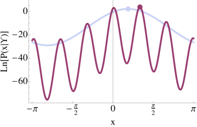
Figure 4: For a given population response $\Upsilon$, measured when a stimulus $x=0$ is presented, the error of a multi-scale code can be worse than that of a single-scale code. A particular population response gives rise to a posterior probability $P(x|\Upsilon)$, an example of which is shown above for a population code with $M=8$, $f_{max}\tau=1$ and $\sigma^{2}=0.86$. The maximum likelihood estimate $\hat{x}$ in this example is 0.59 for a single module (light blue), and 1.05 for two modules (pink)–these are indicated by dots marking the highest peaks, respectively. Compared to a single module, the expected error $\left\langle(x-\hat{x})^{2}\right\rangle$ is five times larger when using two modules.

Consider a two-scale population code, as in Fig. 3. As a first approximation to the typical (or median) error, set $\hat{\mu}_{i}$ and $\hat{\kappa}_{i}$ to their expected values in Eq. 10; later, we will refine the numerical computation to reflect the true average error. As $\lambda_{1}$ is made smaller relative to $\lambda_{0}$, the typical error improves initially, but then worsens as $\lambda_{1}$ falls below the resolution of the module with length scale $\lambda_{0}$. For $\lambda_{1}\ll\lambda_{0}$, $P\left(x-\hat{\mu}\right)$ develops side peaks at integer multiples of $2\pi/\lambda_{1}$ (Fig. 3a); the expected typical error worsens. In the example shown, $1/\sqrt{J}\approx 16.6$, so we deduce that the Cramér-Rao bound of Eq. (5) can be attained for safety factors $S>5$ (Fig. 3b). For $\lambda_{0}/\lambda_{1}\to\infty$, the resolution of the population code with two modules reverts to that of the single (coarse-scale) module.

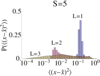
(a)

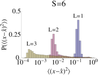
(b)

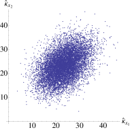
(c)

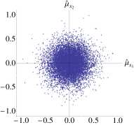
(d)

Figure 5: Multiple modules can refine the estimate of $x$, decreasing the error by more than an order of magnitude for each new module added (Fig. 5a). The maximum likelihood estimate of $\hat{\bm{x}}\in[-\pi,\pi)^{3}$ and the posterior distribution $P((x-\bm{x})|\bm{\Upsilon})$ are evaluated numerically for each sampled population response $\bm{\Upsilon}$. The top panels show the distribution of expected errors for population codes with $L=1,2,$ and 3 modules encoding $\bm{x}$ at different spatial scales. Every module contains $M=8^{3}=512$ neurons with tuning curves that are equidistantly spaced. The relative tuning width is $\sigma^{2}=0.86$ for each neuron, and Eq. (9) dictates the geometric progression of spatial scales. When $S=5$, the refinement scheme breaks down by the third module ($L=3$, Fig. 5b). The errors have been sampled 10,000 times. For a multi-dimensional stimulus $\bm{x}$, the posterior probability $P(\bm{x}|\Upsilon)$ depends on the random variables $\hat{\kappa}_{x_{\alpha}}$ and $\hat{\mu}_{x_{\alpha}}$along the different dimensions. The random variables $\hat{\kappa}_{x_{\alpha}}$ are correlated (Fig. 5c), with a pairwise correlation of 0.44. This correlation depends on $\sigma^{2}$ and $f_{\max}\tau$, and can be stronger or weaker. In contrast, the random variables $\hat{\mu}_{x_{\alpha}}$ are uncorrelated (Fig. 5d).

Going beyond the first-order approximation, we can sample the network’s response $\bm{\Upsilon}$ repeatedly, and thereby sample $\hat{\kappa}_{i}$ and $\hat{\mu}_{i}$. Numerically, we can thus estimate the average error of the population code from Eq. (10) without resorting to averaging $\hat{\kappa}_{i}$, even for multi-dimensional stimuli with $D>1$. We proceed in three steps: first, we numerically determine the maximum a posteriori estimate $\hat{\bm{x}}$ of ${\bm{x}}$ by maximizing the argument in the exponential of Eq. (10); secondly, we integrate over the posterior distribution to obtain the expected error ${\left\langle\left(\bm{x}-\bm{\hat{}}{\bm{x}}\right)^{2}\right\rangle}_{P(\bm{x}|\Upsilon)}$ for each response $\bm{\Upsilon}$; lastly, we build a histogram of the expected errors.

The posterior probability in Eq. (10) depends on the superposition of oscillatory functions in the argument to the exponential function. Decoding the population response $\Upsilon$ can lead to combinations of $\hat{\mu}_{i}$’s and $\hat{\kappa}_{i}$’s that cause the oscillatory functions to interfere constructively, but at the wrong location; witness Fig. 4, in which the MAP estimate of $x$ actually becomes worse when using a second module to refine the estimate from the first one.

For multidimensional stimuli $\bm{x}$ with $D>1$, the risk of catastrophic error is cumulative, as each new dimension adds a new possibility to make a decoding mistake. As the dimension $D$ or the number of modules $L$ increases, the requirement that $S\gg 1$ must be made more stringent.

We numerically analyze a multi-scale population code for a stimulus $\bm{x}$ of dimension $D=3$, so that $\bm{x}$ is contained in the normalized interval $[-\pi,\pi)^{D}$. The network has $M=8^{D}$ neurons with tuning curves that are the product of one-dimensional von Mises functions $\Omega_{i}(\bm{x})=\prod_{\alpha=1}^{D}\Omega_{i}(x_{\alpha})$. For $D\geq 3$, there is an optimal $\sigma^{2}$ for the tuning curve that maximizes the Fisher information Mathis et al. (2012b); we use the value of $\sigma^{2}\approx 0.86$ appropriate for $D=3$. If one takes a marginal safety factor $S=6$ in Eq. (9), the errors decrease by more than an order of magnitude for each new module added, as predicted by the Fisher information’s scaling as $J^{L}$ (Fig. 5a); adding neurons to a single module (at a single spatial scale), in contrast, leads only to an improvement that is linear in $N$. As one decreases the safety factor to $S=5$, catastrophic errors accumulate; Fig. 5b shows that the third module does not improve the average error. Although the posterior probability factorizes in the $D$ dimensions, the components of $\hat{\kappa}$ along these dimensions are correlated (Fig. 5c). Hence, decoding a population response that is uncertain in $x_{1}$, say, will also likely be uncertain in $x_{2}$ and $x_{3}$. As for the single-scale population code (see Fig. 2), the expected error as a function of the response $\Upsilon$ can be greater or less than the inverse Fisher information $1/J$. On average, though, the expected error of the MAP estimate is bounded from below by $1/J$, and for $S>5$ the bound is close to the average error.

III Population coding model with noise correlations

Until now, we have considered a network of $N$ neurons in which the fluctuations in neuronal activity depend only on the stimulus $x$, not on the activity of other neurons. We now treat the more general case of neuronal activity that has non-trivial correlation structure. Correlations might adversely affect the Fisher information and potentially even make a multi-scale code for cortex infeasible.

Before estimating the noise correlations for real spike trains from grid cells recorded in entorhinal cortex, let us extend the standard model for ensembles of correlated cells with unimodal tuning curves Shamir and Sompolinsky (2006); Ecker et al. (2011) to grid codes. To keep the analysis simple, we consider only a one-dimensional stimulus $x\in[-\pi,\pi)$, and compare the Fisher information to the mean squared error.

III.1 Model of noise correlations

In the equation for the response of neuron $i$, $\Upsilon_{i}(x)=\Omega_{i}(x)+\eta_{i}(x)$, let $\eta_{i}(x)$ now follow a multivariate normal distribution with zero mean and a non-diagonal covariance matrix $Q(x)$, which implies that the neurons are no longer statistically independent. More specifically, let us posit the model in Ref. Ecker et al. (2011), for which the covariance matrix is given by the product

$$Q_{ij}(x)=\sqrt{\Omega_{i}(x)}\cdot r_{ij}\cdot\sqrt{\Omega_{j}(x)}.$$ (11)

This model assumes that the correlation factor between two neurons $r_{ij}$ is independent of the stimulus $x$, hence $Q_{ij}(x)$ quantifies the ”noise correlations”. In the limit in which neurons become statistically independent, $r_{ij}=\delta_{ij}$, $Q_{ij}(x)=\Omega_{i}(x)\delta_{ij}$; in other words, the variance scales with the mean response $\Omega_{i}(x)$, just as in the discrete Poisson model.

To complete the model, we need to determine the correlation coefficients $r_{ij}$. Within a module, each cell’s tuning curve has a spatial phase $\varphi_{i}$. The functional organization of cortex Ecker et al. (2011) suggests that cells with similar coding properties will have larger correlation coefficients; this is, indeed, the case for grid cells in cortex, as we will show in detail later. Therefore, we let the correlation coefficient between two cells depend on the difference $d$ in spatial phases $\varphi_{i}$ and $\varphi_{j}$:

$$r_{ij} = c\left(-\pi+(\varphi_{i}-\varphi_{j}+\pi)\!\!\!\mod 2\pi)\right)$$ (12)

$$+\delta_{ij}(1-c(0)).$$

Here $c$ is a monotonically decreasing function. We will use $c(d)=c_{0}\displaystyle\cdot\exp\left(-\frac{d}{\nu}\right),$ with $\nu=1$. Across modules the correlations are assumed to vanish.

III.2 Fisher information for correlated populations

For the model of Eq. (11)-(12), the Fisher information can be written as a sum Kay (1993); Shamir and Sompolinsky (2006); Ecker et al. (2011):

$$J(x)=J_{mean}(x)+J_{cov}(x)$$ (13)

with the following individual parts:

$$J_{mean}(x)=(\Omega^{\prime}(x))^{t}Q(x)^{-1}\Omega^{\prime}(x)$$ (14)

$$J_{cov}(x)=\frac{1}{2}\mathrm{Tr}\left(\left(Q^{\prime}(x)Q(x)^{-1}\right)^{2}\right).$$ (15)

In these equations, $\Omega^{\prime}$ and $Q^{\prime}$ are the derivatives with respect to the stimulus variable $x$. $J_{mean}$ depends on the changes of the mean firing rate $\Omega^{\prime}$ and $J_{cov}$ depends on changes in the covariance structure $Q^{\prime}$.

We will compare the Cramér-Rao estimate of the error based on the Fisher information to the least mean square estimator (MSE) for the neural population code. The latter is given by

$$\widehat{x_{MSE}}(K)=\frac{\int_{-\pi}^{\pi}xP(K|x)dx}{\int_{-\pi}^{\pi}P(K|x)dx}.$$ (16)

Numerically, we divided the stimulus space $[-\pi,\pi)$ into $m=10^{5}$ equidistant points $\{x_{0},x_{1},\ldots,x_{m}\}$ and computed the MSE for $n=15,000$ uniformly distributed positions. After averaging over the squared residues, one obtains the mean square (estimate) error:

$$\epsilon_{MSE}^{2}=1/n\sum_{k}(\widehat{x_{MSE}}(K(x_{k})))-x_{k})^{2}.$$ (17)

III.3 Correlations in multi-
and single-scale population codes

We studied how the Fisher information $J$ depended on the population size $N$ and the correlation peak $c_{0}$, either by increasing the number of modules $L$ or by adding multiples of $M$ neurons to a single module. For the simulations, we set the peak rate to $f_{max}=20$ Hz and the tuning width to $\sigma^{2}=1/2$. Qualitatively these choices are not crucial, as long as there are enough neurons to cover the space given $\sigma$ and the peak spike count is larger than one (cf. Ref Mathis et al. (2012b)).

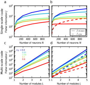
Figure 6: Fisher information for population codes with correlations. We evaluated the Fisher information at position $x=0$. a: The total Fisher information $J$ for a population of $N$ place cells with correlation peak $c_{0}$. For zero-correlation the Fisher information grows linearly in $N$. For larger correlation coefficients the Fisher information falls, but eventually grows linearly in $N$, as indicated by considering the two components of $J$ individually, see subfigure b. b: The same simulation, but the two parts of the Fisher information $J_{mean}$ and $J_{cov}$ are shown separately in solid and dashed lines, respectively. The mean term saturates for increasing correlation peak $c_{0}$, but the covariance term grows linearly and is in fact independent of the correlation peak $c_{0}$. c: Fisher information for grid code without inter-module correlation. The total Fisher information $J$ for a population of $L$ modules and correlation peak $c_{0}$. Each module contains $M=200$ neurons. Even for increasing correlation, the population Fisher information still grows stronger than linearly. The stronger the correlation coefficient becomes the smaller the contraction factor $C/\sqrt{J}$ becomes, and therefore the smaller the growth. d: The same simulation, but the two parts of the Fisher information $J_{mean}$ and $J_{cov}$, are shown separately in solid and dashed lines, respectively.

In the absence of noise correlations, the Fisher information of a single module grows linearly in $N$ Zhang and Sejnowski (1999); Mathis et al. (2012a). For rising correlation amplitude $c_{0}$, the Fisher information decreases, yet still grows linearly with $N$ (Figure 6a). This effect can be explained by considering the two components $J_{mean}$ and $J_{cov}$ individually, as shown in Fig. 6b. While the former saturates, the latter grows linearly in $N$, independently of the degree of correlation. This result is well known, e.g., see Shamir and Sompolinsky Shamir and Sompolinsky (2006); Ecker et al. (2011).

For a nested, multi-scale population code, the Fisher information in each module decreases as the peak intra-module correlation $c_{0}$ increases. For $c_{0}=0$, the spatial periods should obey the previously derived relationship for the population code to attain the Cramér-Rao bound:

$$\lambda_{k+1}=\frac{S\cdot\lambda_{k}}{\sqrt{J}},$$ (9)

with safety factor $S\gg 1$ and $J$ the Fisher information of the first module (at the coarsest scale, see Mathis et al. (2012a), Eq. 8 and discussion thereof). The same still holds true for $c_{0}>0$, only the factor $\sqrt{J}$ is less. Thus, the population Fisher information of a grid code, despite still growing exponentially, grows more slowly in $N$ for rising $c_{0}$. Figures 6c and d depict the Fisher information of a grid code with up to $5$ modules and $M=200$ neurons per module.

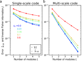
Figure 7: Inverse Fisher information $1/J$ and $\epsilon_{MSE}^{2}$ for an ensemble of cells with tuning curves on a single scale (left) and on multiple scales (right), for varying degrees of noise correlation between neurons in a module. Each ensemble contains $L\cdot M$ equi-distantly arranged neurons, with $M=64$, $f_{max}=10\,\text{Hz}$, and $\sigma^{2}=1/2$. For a pair of neurons, the noise correlation depends on the difference of their preferred phases, according to Eq. (12), with $\nu=0.19$ and varying $c_{0}$. There are no noise correlations between modules. a: each module contains tuning curves of period $\lambda_{0}$. b: the periods are staggered according to Eq. (9) with $S=10$. For the parameters considered here, the MSE is close to the Cramér-Rao bound.

Under certain conditions the Cramér-Rao bound is not tight Bethge et al. (2002); Berens et al. (2011); Mathis et al. (2012b), so we corroborated our results by computing the mean square error (MSE) for these population codes. Figure 7 shows that the MSE is close to the inverse Fisher information for this set of parameters.

IV Noise correlations of biological grid cells

IV.1 Estimation of spatial period, phase and noise correlation in pairs of grid cells

To estimate the correlations between in a real neural population with multi-scale coding properties, we analyzed grid cell data recorded by Hafting et al. (Hafting et al. (2008), available at http://www.ntnu.no/cbm/moser/gridcell). As the experimental methods are extensively covered in the original publication Hafting et al. (2008), we briefly summarize the details relevant to our study here. In the experiments, rats ran back and forth for ten minutes on a $320$ cm long and $10$ cm wide linear track; during each run, the trajectory was tracked using a head-fixed light emitting diode, and the neuronal activity in the medial entorhinal cortex (mEC) was recorded using extracellular tetrodes. From these signals, spike times of several single cells in mEC were isolated. A subset of these cells fired at multiple, periodically spaced locations on the linear track, separated by stretches of the track on which the cells did not fire (Fig. 8). These cells are called ’grid cells’ and exhibit different spatial periods in their firing rate maps.

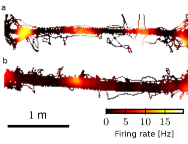
Figure 8: Firing rate maps $\Omega_{i}(x,y)$ for two neurons in the data set from Hafting et al. Hafting et al. (2008), in which rats ran back and forth on a linear track. We filtered the spikes as described in Eq. (18). Cells in a and b differ in their spatial periods, which we estimated to be $88$ and $177$ cm, respectively, from the first peak in the autocorrelation. Prior to the runs on the track, these cells were recorded while the rat foraged in a two-dimensional enclosure, which revealed that the cells had a hexagonal map of spatial firing. It is not guaranteed, however, that the track is aligned to one of the principal axes of the hexagonal map’s lattice, so not all cells have a linear track firing rate $\Omega_{i}(x,y)$ that is perfectly periodic (see also Ref. Domnisoru et al. (2013); Kempf et al. (2012).

The spatial firing of a grid cell is characterized by its spatial period (i.e. average peak-to-peak distance of firing fields) and phase (position of the first peak, for instance, relative to a reference point.) Hafting et al. (2005). Neighboring cells in mEC tend to have a similar spatial period in their firing pattern, but differ in their spatial phases Hafting et al. (2005).

Overall, the data set contained $97$ cells. Left- and rightward runs were treated separately, as the cell’s firing pattern for the two directions was often different (see, for instance, Fig. 8a). As is common practice Hafting et al. (2008); Brun et al. (2008), we excluded the first $30\,\text{cm}$ on both sides of the linear track from consideration; here the rats slow down and turn around. For pairs of grid cells that were recorded at the same time and in the same animal, we estimated the noise correlations and the phase difference between the firing patterns. $302$ such pairs were analyzed. The phase difference of two periodic signals only exists if their frequencies are similar. The spatial period of each grid cell must be estimated from spike trains that are variable from run to run, so we proceed as follows:

• we determine the firing rate for each cell by Gaussian kernel filtering in the spatial domain:

  $$\Omega(x,y)=\frac{\sum_{s}\exp{\left(-\frac{(s_{x}-x)^{2}}{2\sigma_{x}^{2}}-\frac{(s_{y}-y)^{2}}{2\sigma_{y}^{2}}\right)}}{dT\sum_{t}\exp{\left(-\frac{(\gamma_{t}(x)-x)^{2}}{2\sigma_{x}^{2}}-\frac{(\gamma_{t}(y)-y)^{2}}{2\sigma_{y}^{2}}\right)}}$$ (18)

  where $s=(s_{x},s_{y})\in S$ are the spike positions. $\gamma_{t}$ is the discretized trajectory, sampled in $dT=0.02\,\text{s}$ steps. We used $\sigma_{x}=3\,\text{cm}$ and $\sigma_{y}=3\,\text{cm}$. The map of Eq. (18) was computed on a discretized grid with $N_{x}\times N_{y}=160\times 10$ bins denoted by $(x_{k},y_{l})_{\{1\leq k\leq N_{x},1\leq l\leq N_{y}\}}$ (see Fig. 8b). Then we averaged along the $y$ axis and obtained the firing rate profile $\Omega_{i}(x_{k})$ for $1\leq k\leq N_{x}$ and each cell $i$.

• The spatial period $\lambda_{i}$ is defined as the first peak in the autocorrelogram of the firing map $\Omega_{i}(x_{k})$.

• For each cell pair $(i,j)$ we compute the cross-correlogram of $\Omega_{i}(x_{k})$ and $\Omega_{j}(x_{k})$, and the spatial period $\lambda_{ij}$ as the first peak in the cross-correlogram.

• If $\lambda_{ij}$ differs by maximally $20\%$ from both $\lambda_{i}$ and $\lambda_{j}$, we assume that the cells are from the same module (i.e. share the spatial period) and define their phase difference $\widehat{\varphi_{ij}}$ as the position of the peak in the cross-correlogram modulo $\lambda_{ij}$.

• Then we define the relative phase difference $\varphi_{ij}=2\pi\cdot\widehat{\varphi_{ij}}/\lambda_{ij}-\pi\in[-\pi,\pi]$.

For each pair $i,j$, we compute the noise correlations as follows:

• From the spike times$t_{k}^{(j)}$ of each neuron $j$ we compute the temporal firing rate by Gaussian kernel filtering:

  $$f_{j}(t)=\frac{1}{\sqrt{2\pi}\sigma}\sum_{k}\exp{\left(-\frac{(t_{k}^{(j)}-t)^{2}}{2\sigma^{2}}\right)}$$ (19)

  We used $\sigma=20\,\text{ms}$ and evaluated the firing rate on a $1\,\text{ms}$ fine temporal grid.

• We discretize the environment in $N_{x}\times N_{y}=160\times 10$ bins denoted by $(x_{k},y_{l})_{\{1\leq k\leq N_{x},1\leq l\leq N_{y}\}}$. For each session we compute the entry and exit times into these bins. Thus for each bin $(k,l)$ we get a list of $S_{k,l}$ trajectory segments $\gamma_{k,l}^{s}$ denoting the s-th path trough the bin with entry time $\alpha_{k,l}^{s}$ and exit time $\omega_{k,l}^{s}$.

• We compute the average firing rate for each cell $j$ and path segment $s$:

  $$\overline{F_{k,l}^{j,s}}=\frac{\int_{\alpha_{k,l}^{s}}^{\omega_{k,l}^{s}}f_{j}(t)dt}{\omega_{k,l}^{s}-\alpha_{k,l}^{s}}.$$ (20)

• These rates allow us to compute the noise correlation of cell $i$ and $j$ in each bin $(k,l)$ by computing the correlated response fluctuations around the means:

  $$c^{i,j}_{k,l}=\frac{\mathbb{C}ov_{s}\left(\overline{F_{k,l}^{j,s}},\overline{F_{k,l}^{i,s}}\right)}{\sqrt{\mathbb{V}_{s}\left(\overline{F_{k,l}^{i,s}}\right)\cdot\mathbb{V}_{s}\left(\overline{F_{k,l}^{j,s}}\right)}}.$$ (21)

• These values per bin are then averaged over all bins to get the noise correlations of cell $i$ and $j$:

  $$c_{i,j}=\frac{1}{N_{x}N_{y}}\sum_{k,l}c^{i,j}_{k,l}.$$ (22)

IV.2 Estimated noise correlations of grid cells

In $87$ of $302$ grid cell pairs, both neurons belonged to the same module; i.e., they shared a common spatial period. We computed the noise correlations and relative phases for these $87$ pairs (in $15$ pairs, both neurons were recorded on the same tetrode). The relationship of noise correlation to phase difference is shown in Fig.   9. A least mean squares fit of $c_{0}\exp(-|\varphi|/\nu)$ to the data yielded $c_{0}=0.32$ and $\nu=0.18$. There are $62$ pairs with dissimilar phases (defined as $|\varphi|>0.36=2\nu)$). This group has a mean noise correlation value of $-0.021\pm 0.0006$ (mean $\pm$ standard error of mean). These neurons are, hence, uncorrelated. For similar phases, the maximal noise correlation reaches $0.8$; on average, it is $0.24\pm 0.01$ for the other $25$ pairs. These data indicate that the noise correlations fall the farther apart the spatial phases are.

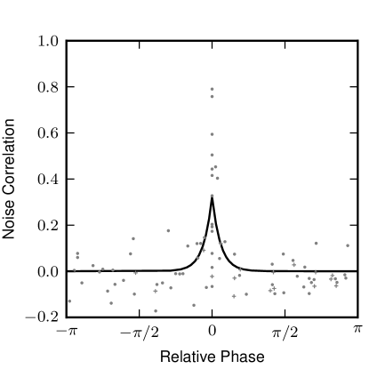
Figure 9: Noise correlation $c_{i,j}$ vs. relative phases $\varphi_{i,j}$ of $87$ pairs of grid cells from the same experimental session as described in the main text. Gray dots indicate pairs from different tetrodes and gray crosses from the same tetrode, respectively. Black continuous line is a least-mean-square fit of the function $c_{0}\exp(-|\varphi|/\nu)$ with values $c_{0}=0.32$ and $\nu=0.18$.

V Conclusion

A common objection raised to using the Fisher information is that it only provides a bound to the resolution of the population code. When the response is discrete or sampled for short durations, this bound is not attainable by maximum likelihood decoding Bethge et al. (2002); Berens et al. (2011); Mathis et al. (2012b). In multi-scale codes, the ratio of successive scales $\lambda_{k+1}/\lambda_{k}$ determines whether the Fisher information is appropriate: if this ratio satisfies Eq. 9 with $S>5$, the Fisher information estimate will be tight. Here we showed how maximum likelihood estimation for a multi-scale population code with circular Gaussian (von Mises) tuning curves (Eq. (2)) can be solved exactly, providing independent confirmation of the ideal scaling ratios. For each response, one can thus not only estimate the most likely stimulus, but also gauge how reliable the estimate is—the Fisher information only measures the average reliability under ideal conditions. If the stimulus comes from the senses, such as vision or hearing, the range of stimulus intensities can cover many orders of magnitude; by having neurons in a population with different scales of sensitivity, the network can match its response to the dynamic range of the stimulus. But even when the dynamic stimulus range does not extend over many orders of magnitude, the explicit maximum likelihood solution shows that a multi-scale code is feasible, straightforwardly decodable, and advantageous.

Furthermore, we demonstrated that noise correlations at each scale reduce the Fisher information in a nested grid code, but that the resolution still scales as $J^{L}$, where $J$ is the Fisher information of a single module and $L$ is the number of modules (each with a different scale). Within a single module, the resolution scales linearly with the number of neurons $M$, with or without noise correlations Shamir and Sompolinsky (2006); Ecker et al. (2011).

We measured the noise correlations in the spike trains from grid cells in the medial entorhinal cortex (mEC) of rats running on a one-dimensional, linear track Hafting et al. (2008). As in other studies in the visual Ecker et al. (2010) and olfactory cortices Miura et al. (2012) we find that the mean noise correlation of a random pair of neurons practically vanishes. However, when two grid cells have highly overlapping firing fields, so that both the spatial period and the phase are similar, the noise correlations reach values of up to $0.8$. We can imagine four different causes for such comparatively high correlations: (i) grid cells in mEC mutually entrain to the theta rhythm, a 5-12 Hz network rhythm present throughout hippocampus, subiculum, and the entorhinal cortex. Grid cell spikes precess with respect to this rhythm, so that the spike phase relative to the theta rhythm shifts continuously and predictably, from the time that the animal enters a firing field of a cell until the time it leaves that field Hafting et al. (2008); Reifenstein et al. (2012). If two neurons have overlapping firing fields, similar theta phase precession could lead to high noise correlation. (ii) common external input (e.g. from hippocampus Bonnevie et al. (2013), or from other brain areas van Strien et al. (2009)) (iii) recurrent intrinsic connections between neurons in mEC (e.g. Beed et al. (2010); Burgalossi et al. (2011); Couey et al. (2013); Beed et al. (2013)) (iv) the spike trains have been acquired by spike-sorting extracellular recordings Hafting et al. (2008); this process possibly falsely assign spikes from the same neuron to different neurons and vice versa Lewicki (1998), which can lead to spurious noise correlations.

Noise correlations are higher between neurons with similar tuning curves; this can have a strong effect on the coding precision of population codes – and nested grid codes are no exception. Previous studies focused on ensembles of cells with unimodal tuning curves Abbott and Dayan (1999); Shamir and Sompolinsky (2001); Wilke and Eurich (2001); Shamir and Sompolinsky (2006); Ecker et al. (2011) rather than ensembles with multimodal tuning curves, such as grid cells. Interestingly, if one makes unimodal tuning curves heterogeneous by varying the tuning widths and peak firing rates across neurons, reducing the noise correlations does not improve encoding accuracy Wilke and Eurich (2001); Shamir and Sompolinsky (2006); Ecker et al. (2011). Grid cells are also highly heterogeneous in their firing rates and tuning parameters Hafting et al. (2005); Herz et al. (2011), but how heterogeneity would affect the Fisher information has not been studied.

We have assumed that the signal itself is not subject to noise. If one adds adiabatic noise to $x$, so that $y=x+\xi$, then the population encodes $y$ instead of $x$ to a certain precision, and one obtains $\left\langle{\left(x-\hat{x}\right)}^{2}\right\rangle\sim J^{-1}+\left\langle\xi^{2}\right\rangle$. While a coding strategy that uses multiple scales will still be superior, the law of diminishing returns applies—reducing $J^{-1}$ far below $\left\langle\xi^{2}\right\rangle$ makes little sense. It is intuitive that the resolution at the coarsest scale should limit the next length scale, but the resolution itself is sensitive to many parameters, such as the peak firing rate and the number of neurons with tuning curves at the coarsest scale. To minimize the number of spurious solutions in decoding the neuronal response, a conservative approach might involve taking $1/2<\lambda_{k+1}/\lambda_{k}<1$, independently of the resolution at scale $\lambda_{k}$. Maximum likelihood decoding of a multi-scale population code relies on the constructive interference of spatial oscillations with periods $\lambda_{k}$ and $\lambda_{k+1}$, which combine near the true stimulus $x$ to yield a high posterior probability of the stimulus given the response (see Eq. (10)); any other instances of constructive interference can lead to decoding errors. If the Fisher information is at least $\sqrt{J}\sim\lambda_{k}$, then limiting $1/2<\lambda_{k+1}/\lambda_{k}<1$ will limit the probability of the oscillations on the two scales constructively interfering again within $\lambda_{k}$ of the true stimulus $x$. The ratio of scales observed in experimental data seems to be in accordance with $0.6<\lambda_{k+1}/\lambda_{k}<0.8$ Barry et al. (2007); Stensola et al. (2012).

Other authors have suggested that the different periods should not be simple multiples of each other Burak et al. (2006); Gorchetchnikov and Grossberg (2007); Fiete et al. (2008); Sreenivasan and Fiete (2011); in the absence of noise, each $x$ would then give rise to a unique pattern of population activity $\Upsilon$, up until $x$ reaches the least common multiple of all the periods. Hence, a much larger range of $x$ can be encoded. Such a strategy is called modular arithmetic Burak et al. (2006); its main drawback, though, is its susceptibility to noise Fiete et al. (2008); Sreenivasan and Fiete (2011); Mathis et al. (2012b). When $x$ evolves continuously in time, error correction could be used to counteract this noise Sreenivasan and Fiete (2011). But even if $x$ has no continuous history dependence, a modular arithmetic code is feasible, provided $M$ is sufficiently large—the specific model of Eq. (2) is explicitly solved by Eq. (10) for any set of spatial periods $\lambda_{i}$, so one can make the expected error arbitrarily small as long as one increases $N$. The authors of Ref. Wei et al. (2013) set themselves the opposite goal and try to minimize $N$; by using scaling arguments and dimensional analysis, they derive optimal parameters for a multi-scale code.

These authors and we have treated the comparatively straightforward problem of encoding $x\in I\subset\mathds{R}^{D}$ using multiple scales. If instead the neuronal population represents the probability of a stimulus $p(x)$ instead of just the estimate of $x$ Pouget et al. (2000), then a multi-scale encoding becomes analogous to a Fourier decomposition of the probability distribution, given the similarity between the set of periodic tuning curves at different length scales and the Fourier basis. The analogy is approximate, though, as the corresponding ”Fourier coefficients” would be highly stochastic given the inherent randomness in the neuronal response; moreover, the set of tuning curves is not complete. A more detailed analysis of probabilistic coding models in the context of multiple scales awaits investigation; our result that the uncertainty in the position estimate fluctuates strongly as a function of the response, may be a first step in this direction.

References

- Mathis et al. (2012a) A. Mathis, A.V.M. Herz, and M.B. Stemmler, Physical Review Letters 109, 018103 (2012a).
- Haar (1909) A. Haar, Mathematische Annalen 69, 331 (1909).
- Chui (1992) C. K. Chui, An introduction to wavelets (Academic Press Professional, Inc., San Diego, CA, USA, 1992).
- Unser and Aldroubi (1996) M. Unser and A. Aldroubi, Proceedings of the IEEE 84 (1996).
- Mallat (2009) S. Mallat, A Wavelet Tour of Signal Processing The sparse way, 3rd ed. (Elsevier Inc., 2009).
- Acharaya and Tsai (2005) T. Acharaya and P. Tsai, Image (Rochester, N.Y.) (John Wiley & Sons, 2005).
- Simoncelli et al. (1992) E. P. Simoncelli, W. T. Freeman, E. H. Adelson, and D. J. Heeger, IEEE Trans Information Theory 38, 587 (1992).
- Riesenhuber and Poggio (1999) M. Riesenhuber and T. Poggio, Nature Neurosci. 2, 1019 (1999).
- Hubel and Wiesel (1968) D. Hubel and T. Wiesel, Journal of Physiology 195, 215 (1968).
- DeValois and DeValois (1990) R. DeValois and K. DeValois, Spatial Vision (Oxford University Press, USA, 1990) p. 402.
- Olshausen and Field (1996) B. Olshausen and D. Field, Nature 381 (1996).
- Lewicki (2002) M. Lewicki, Nature Neuroscience 5, 356 (2002).
- Hafting et al. (2005) T. Hafting, M. Fyhn, S. Molden, M. Moser, and E. Moser, Nature 436, 801 (2005).
- Boccara et al. (2010) C. Boccara, F. Sargolini, V. Thoresen, T. Solstad, M. Witter, E. Moser, and M. Moser, Nature Neuroscience 13, 987 (2010).
- Barry et al. (2007) C. Barry, R. Hayman, N. Burgess, and K. Jeffery, Nature Neuroscience 10, 682 (2007).
- Stensola et al. (2012) H. Stensola, T. Stensola, T. Solstad, K. Frø land, M.-B. Moser, and E. Moser, Nature 492, 72 (2012).
- Mathis et al. (2012b) A. Mathis, A. Herz, and M. Stemmler, Neural Computation 24, 2280 (2012b).
- Wei et al. (2013) X.-X. Wei, J. Prentice, and V. Balasubramanian, arXiv:1304.0031v1 (2013).
- Seung and Sompolinsky (1993) H. Seung and H. Sompolinsky, Proceedings of the National Academy of Sciences 90, 10749 (1993).
- Zhang and Sejnowski (1999) K. Zhang and T. Sejnowski, Neural Computation 11, 75 (1999).
- Wilke and Eurich (2001) S. Wilke and C. Eurich, Neural Computation 189, 155 (2001).
- Bethge et al. (2002) M. Bethge, D. Rotermund, and K. Pawelzik, Neural Computation 14, 2317 (2002).
- Brown and Bäcker (2006) W. Brown and A. Bäcker, Neural Computation (2006).
- McDonnell and Stocks (2008) M.D. McDonnell and N.G. Stocks, Physical Review Letters 101, 058103 (2008).
- Nikitin et al. (2009) A.P. Nikitin, N.G. Stocks, R.P. Morse, and M.D. McDonnell, Physical Review Letters 103, 138101 (2009).
- Zohary et al. (1994) E. Zohary, M. Shadlen, and W. Newsome, Nature (1994).
- Schneidman et al. (2006) E. Schneidman, M. Berry, R. Segev, and W. Bialek, Nature 440, 1007 (2006).
- Ecker et al. (2010) A. Ecker, P. Berens, G. Keliris, M. Bethge, N. Logothetis, and A. Tolias, Science (New York, N.Y.) 327, 584 (2010).
- Cohen and Kohn (2011) M. Cohen and A. Kohn, Nature Neuroscience 14, 811 (2011).
- Lee et al. (1998) D. Lee, N. Port, W. Kruse, and A. Georgopoulos, Journal of Neuroscience 18, 1161 (1998).
- Smith and Kohn (2008) M. Smith and A. Kohn, Journal of Neuroscience 28, 12591 (2008).
- Miura et al. (2012) K. Miura, Z. Mainen, and N. Uchida, Neuron 74, 1087 (2012).
- Abbott and Dayan (1999) L. Abbott and P. Dayan, Neural Computation 11, 91 (1999).
- Shamir and Sompolinsky (2001) M. Shamir and H. Sompolinsky, NIPS 15, 277 (2001).
- Shamir and Sompolinsky (2006) M. Shamir and H. Sompolinsky, Neural Computation 18, 1951 (2006).
- Ecker et al. (2011) A. Ecker, P. Berens, A. Tolias, and M. Bethge, Journal of Neuroscience 31, 14272 (2011).
- Hafting et al. (2008) T. Hafting, M. Fyhn, T. Bonnevie, M. Moser, and E. Moser, Nature 453, 1248 (2008).
- Yaeli and Meir (2010) S. Yaeli and R. Meir, Frontiers in Computational Neuroscience 4, 130 (2010).
- Dayan and Abbott (2001) P. Dayan and L. Abbott, Theoretical Neuroscience: Computational and Mathematical Modeling of Neural Systems (MIT Press, 2001).
- Georgopoulos, Schwartz and Kettner (2001) A. Georgopoulos, A. Schwartz, and R. Kettner, Science (New York, N.Y.) 233, 1416-19 (1986).
- Note (1) For , one computes a characteristic function . The characteristic function allows one to compute the moments of (by taking the -th derivative of at ). We then expand the modified Bessel functions asymptotically to get the scaling result in the text.
- Kay (1993) S. Kay, Fundamentals of Statistical Signal Processing: Estimation Theory (Prentice Hall, Upper Saddle River, New Jersey, 1993).
- Berens et al. (2011) P. Berens, A. Ecker, S. Gerwinn, A. Tolias, and M. Bethge, Proceedings of the National Academy of Sciences (2011).
- Note (2) For a few cells, multiple long sessions were recorded, but we only used the first for each cell for this analysis.
- Domnisoru et al. (2013) C. Domnisoru, A. A. Kinkhabwala, and D. W. Tank, Nature 495, 199 (2013).
- Kempf et al. (2012) F. M. Kempf, A. Mathis, M. Stemmler, and A. V. M. Herz, Front. Comput. Neurosci. (2012), 10.3389/conf.fncom.2012.55.00019.
- Brun et al. (2008) V. Brun, T. Solstad, K. Kjelstrup, M. Fyhn, M. Witter, E. Moser, and M. Moser, Hippocampus 18, 1200 (2008).
- Reifenstein et al. (2012) E. Reifenstein, R. Kempter, S. Schreiber, M. Stemmler, and A. Herz, Proceedings of the National Academy of Sciences , 1 (2012).
- Bonnevie et al. (2013) T. Bonnevie, B. Dunn, M. Fyhn, T. Hafting, D. Derdikman, J. Kubie, Y. Roudi, E. Moser, and M.-B. Moser, Nature Neuroscience , 1 (2013).
- van Strien et al. (2009) N. van Strien, N. Cappaert, and M. Witter, Nature reviews. Neuroscience 10, 272 (2009).
- Beed et al. (2010) P. Beed, M. Bendels, H. Wiegand, C. Leibold, F. Johenning, and D. Schmitz, Neuron 68, 1059 (2010).
- Burgalossi et al. (2011) A. Burgalossi, L. Herfst, M. von Heimendahl, H. Förste, K. Haskic, M. Schmidt, and M. Brecht, Neuron 70, 773 (2011).
- Couey et al. (2013) J. Couey, A. Witoelar, S.-J. Zhang, K. Zheng, J. Ye, B. Dunn, R. Czajkowski, M.-B. Moser, E. Moser, Y. Roudi, and M. Witter, Nature Neuroscience , 1 (2013).
- Beed et al. (2013) P. Beed, A. Gundelfinger, S. Schneiderbauer, J. Song, C. Böhm, A. Burgalossi, M. Brecht, I. Vida, C. Leibold, and D. Schmitz, under review (2013).
- Lewicki (1998) M.S. Lewicki, Network: Comput. Neural Syst. 9, R53–R78 (1998).
- Herz et al. (2011) A. Herz, C. Kluger, A. Mathis, and M. Stemmler, in Ninth Göttingen Meeting of the German Neuroscience Society (2011) pp. T26–15C.
- Burak et al. (2006) Y. Burak, T. Brookings, and I. Fiete, arXiv:q-bio/0606005v1 93106, 4 (2006). .
- Gorchetchnikov and Grossberg (2007) A. Gorchetchnikov and S. Grossberg, Neural Networks 20, 182 (2007).
- Fiete et al. (2008) I. Fiete, Y. Burak, and T. Brookings, Journal of Neuroscience 28, 6858 (2008).
- Sreenivasan and Fiete (2011) S. Sreenivasan and I. Fiete, Nature Neuroscience 14, 1330 (2011).
- Pouget et al. (2000) A. Pouget, P. Dayan, and R. Zemel, Nature Reviews Neuroscience 1, 125 (2000).