Ultracold Quantum Gases and Lattice Systems:
Quantum Simulation of Lattice Gauge Theories

Abstract

Abelian and non-Abelian gauge theories are of central importance in many areas of physics. In condensed matter physics, Abelian $U(1)$ lattice gauge theories arise in the description of certain quantum spin liquids. In quantum information theory, Kitaev’s toric code is a ${\mathbb{Z}}(2)$ lattice gauge theory. In particle physics, Quantum Chromodynamics (QCD), the non-Abelian $SU(3)$ gauge theory of the strong interactions between quarks and gluons, is non-perturbatively regularized on a lattice. Quantum link models extend the concept of lattice gauge theories beyond the Wilson formulation, and are well suited for both digital and analog quantum simulation using ultracold atomic gases in optical lattices. Since quantum simulators do not suffer from the notorious sign problem, they open the door to studies of the real-time evolution of strongly coupled quantum systems, which are impossible with classical simulation methods. A plethora of interesting lattice gauge theories suggests itself for quantum simulation, which should allow us to address very challenging problems, ranging from confinement and deconfinement, or chiral symmetry breaking and its restoration at finite baryon density, to color superconductivity and the real-time evolution of heavy-ion collisions, first in simpler model gauge theories and ultimately in QCD.

1 Introduction

Gauge theories play an important role in many areas of physics. In particle physics, Abelian and non-Abelian gauge fields mediate the fundamental strong and electroweak forces between quarks, electrons, and neutrinos. In atomic and molecular physics, electromagnetic Abelian gauge fields are responsible for the Coulomb forces that bind electrons to atomic nuclei. In condensed matter physics, besides the fundamental electromagnetic field, effective gauge fields may emerge dynamically at low energies [1]. For example, in quantum Hall systems, statistical gauge fields endow Laughlin quasi-particles with anyon statistics. Some quantum spin liquids [2], which may arise in geometrically frustrated antiferromagnets, can be described by quantum dimer models [3, 4] which are $U(1)$ lattice gauge theories. Other quantum spin liquids have Abelian ${\mathbb{Z}}(2)$ or non-Abelian $SU(2)$ symmetry, and Kitaev’s toric code [5] provides an example of a ${\mathbb{Z}}(2)$ lattice gauge theory relevant in quantum information theory. Furthermore, universal topological quantum computation is based on non-Abelian Chern-Simons gauge theories [6].

Gauge theories reflect a redundancy in or description of Nature. When we use vector potentials to talk about magnetic fields, we introduce unphysical degrees of freedom, which ultimately decouple thanks to a local gauge symmetry. Similarly, when a condensed matter theorist factorizes an electron field into a charged spinless boson and a neutral fermion carrying the spin, a phase ambiguity arises that again manifests itself as a gauge symmetry. While one may speculate whether Nature herself uses redundant variables at the ultimate cut-off scale, it is not surprising that gauge fields dominate the low-energy domain. In particular, Abelian gauge fields can exist in a Coulomb phase, which provides us with naturally massless photons that mediate the electromagnetic interaction between charges at arbitrarily large distances. Non-Abelian gauge theories [7, 8], on the other hand, are confining and give rise to massive particles. For example, in Quantum Chromodynamics (QCD) [9, 10, 11] with the non-Abelian gauge group $SU(3)$, massless gluons and almost massless quarks are turned into massive hadrons, including protons and neutrons. However, thanks to the property of asymptotic freedom, the hadron masses are exponentially small compared to the ultimate cut-off scale (e.g. the Planck scale), and protons and neutrons hence also naturally participate in the low-energy physics. The robustness of gauge invariance at low energies, even if it is violated at the cut-off scale, has been recognized a long time ago [12]. When gauge theories undergo the Higgs mechanism, the gauge bosons pick up a mass at the scale of the vacuum expectation value of the Higgs field. Particle physicists are puzzled by the fact that the electroweak gauge bosons W and Z as well as the Higgs boson exist far below the Planck scale, because the large mass hierarchy seems to require unnatural fine-tuning. In condensed matter physics, man-made fine-tuning happens on a daily basis. For example, by tuning a sophisticated material to a deconfined quantum critical point, one may hope to liberate an effective gauge boson that would otherwise remain confined and thus unobservable [13].

The omnipresence of gauge fields confronts us with very rich low-energy dynamics that are often difficult to understand. In particular, in strongly coupled materials, such as frustrated quantum magnets, high-temperature superconductors, or dense nuclear matter, perturbative analytic methods fail, and one must resort to numerical calculations. Despite tremendous successes of Monte Carlo simulations in condensed matter and particle physics, these problems remain largely intractable, due to very severe sign problems which prevent the importance sampling method underlying classical and quantum Monte Carlo. Since the dimension of the Hilbert space grows exponentially with the size of a quantum system, simulating it on a classical computer is in general very difficult. While some sign problems are NP-complete [14], and thus believed to be practically unsolvable, the above mentioned sign problems arising in condensed matter and particle physics are probably not of this sort. Still, it may require more than a classical computer to deal with them.

Since the ground-breaking experimental realization of Bose-Einstein condensation [15, 16], the field of atomic, molecular, and optical physics has undergone an impressive rapid development. In particular, the degree to which ultracold atomic systems can be engineered and controlled is truly remarkable. Shor was first to show that, if it existed, a quantum computer would vastly outperform classical computers in the task of prime factorization [17]. Very early on, Cirac and Zoller realized theoretically that trapped ions could be used for quantum computation [18]. The prospect of perhaps being able to build a quantum computer spurred the development of algorithms for the envisioned machines. It was soon realized that cold atoms in optical lattices can also be used as quantum simulators. In this way, Feynman’s vision [19] of simulating complicated physical systems by other well-controlled quantum systems is becoming a reality. Quantum simulators [20] are special purpose quantum computers which are used as digital [21] or analog [22] devices to simulate, for example, strongly coupled quantum systems relevant in condensed matter physics. Quantum simulators have been constructed using ultracold atoms in optical lattices [23, 24], trapped ions [25], photons [26], or superconducting circuits on a chip [27]. The D-wave One Rainer chip is a $4\times 4$ aray of unit-cells each hosting 8 superconducting flux qubits with programmable couplings connecting numerous pairs of qubits. Recently, a 108 qubit system has been used to run a finite-temperature variant of the quantum adiabatic algorithm [28] on random instances of an Ising spin glass Hamiltonian [29]. A comparison with a simulated classical and quantum annealer led the authors of this study to conclude that the D-wave device indeed performs quantum rather than classical annealing, however, as yet without achieving any speed-up compared to classical computation for the problem under consideration. Since it utilizes the superposition of quantum phases in its hardware, a quantum simulator does not suffer from the notorious sign problem. From a condensed matter perspective, this is extremely interesting because highly non-trivial many-body systems, such as geometrically frustrated quantum antiferromagnets [30], various spin liquids, or high-temperature superconductors [31] can perhaps be quantum simulated, despite the fact that the sign problem prevents numerical simulations on classical computers. It was a significant breakthrough, when a non-trivial quantum phase transition separating a Mott insulator (with localized particles) from a superfluid, was first quantum simulated by implementing the Bose-Hubbard model with cold atoms in an optical lattice [32]. The parameters of the system are controlled by varying the depth of the optical potential generated by appropriately tuned laser beams. Since the Bose-Hubbard model does not suffer from a sign problem, it can also be simulated on a classical computer. Using quantum Monte Carlo, in this way the quantum simulator has been accurately validated in comparison to the cold atoms experiments [33]. Thus it has been demonstrated explicitly that accurate quantitative experimental control of the theoretical Bose-Hubbard model has indeed been achieved.

It is natural to ask whether one can also quantum simulate relativistic field theories. A field theory quantum simulator should allow us to control a large number of strongly coupled field degrees of freedom, by engineering appropriate local Hamiltonians. It should enable flexible initial state preparation and precise subsequent time-evolution, followed by final state detection. As usual for quantum systems, by repeating identically prepared experiments many times, one obtains physical results by averaging over them. Quantum simulator constructions already exist for several bosonic [34, 35, 36] and fermionic [37, 38, 39, 40] field theories. Quantum simulators have also been constructed for quantum particles interacting with classical gauge fields. A most exciting development are synthetic background gauge fields, in order to access, for example, the fractional quantum Hall effect or topological insulators with atoms. Such synthetic gauge fields can mimic an external magnetic field [41, 42, 43, 44, 45, 46, 47, 48, 49, 50].

In particle physics, one is dealing, e.g., with $SU(3)$ gluon gauge fields, which are not classical background fields but dynamical quantum fields. When coupled to quark fields, their non-perturbative quantum physics is very successfully described by Wilson’s lattice QCD [51, 52, 53, 54, 55, 56, 57]. Still, some problems remain intractable with this method, because again severe sign problems arise. For example, the hot quark-gluon plasma that is generated in heavy ion collisions at the Relativistic Heavy Ion Collider (RHIC) in Brookhaven or at the Large Hadron Collider (LHC) at CERN undergoes an intriguing real-time evolution that is practically impossible to derive from QCD first principles. Even staying within equilibrium thermodynamics, the critical endpoint of the chiral transition line in the QCD phase diagram, which will be investigated experimentally at the Facility for Antiproton and Ion Research (FAIR) at GSI Darmstadt, is difficult to determine accurately using lattice QCD [58, 59] . Similarly, due to a severe sign problem, the deep interior of neutron stars, which may contain color superconducting quark matter [60, 61] can currently not be addressed non-perturbatively from QCD first principles either. While it is difficult to predict when full QCD quantum simulations with cold atoms might become experimentally feasible, it is timely to work towards this long-term goal [62, 63, 64, 65, 66, 68, 67, 69, 70, 71, 72, 73, 74].

What are realistic short-term goals? Obviously, a quantum simulator should aim at those problems that are inaccessible to classical simulation methods (but still verifiable for certain small-scale instances). This includes all problems involving real-time evolution or the physics at high baryon density. Unlike classical computers, initially quantum simulators will not be precision instruments. In particular, they lack automatic error correction. One should hence concentrate on robust, fault-tolerant phenomena of a qualitative nature, such as the presence or absence of specific phases of strongly coupled high-density matter in Abelian and non-Abelian gauge theories, or specific events that may happen or not happen during real-time evolution. Since one is interested in phenomena inaccessible to analytic perturbative calculations, one will deal with lattice gauge theories, for which continuous space is replaced by a discrete grid of lattice points. Rather than aiming directly at the continuum limit of vanishing lattice spacing, it is more realistic and still extremely interesting to first address the strong coupling lattice dynamics.

In this review, we will approach gauge theories from a particle physics point of view, but we will also draw connections to condensed matter physics and quantum information theory. In section 2, we begin with the simpler case of Abelian gauge theories. In order to address non-perturbative effects, we regularize the theory on a lattice, first following the classical Wilson formulation [51], and then extending the concept of lattice gauge theories to quantum link models [75, 76, 77, 78]. The resulting Abelian gauge theories resemble models of condensed matter physics and quantum information theory. In section 3, we present various constructions of quantum simulators for Abelian gauge theories, and discuss possible experimental realizations. In section 4, we then proceed to non-Abelian gauge theories, first introducing them in the framework of Wilson’s lattice gauge theory, and again extending them to quantum link models. This gives rise to the alternative D-theory formulation of quantum field theory [79], which is well suited for quantum simulation with ultracold atoms. In section 5, we present several quantum simulator constructions of interesting non-Abelian lattice gauge theories. Finally, in section 6, we summarize the current status of gauge theory quantum simulators, give an outlook on possible developments in the foreseeable future, and conclude by discussing what will need to be done to ultimately facilitate quantum simulations of QCD.

2 Abelian Gauge Theories

In this section we consider Abelian gauge theories, starting from classical electrodynamics, and then proceeding from the quantum mechanics of a single particle in a classical electromagnetic background field to the quantum field theory of dynamical Abelian gauge fields. Quantum Electrodynamics (QED) is formulated non-perturbatively, first using Wilson’s lattice regularization. The concept of Abelian lattice gauge fields is then extended to quantum link models, which are well-suited for quantum simulation using ultracold matter. Both digital and analog quantum simulator constructions for ${\mathbb{Z}}(2)$ and $U(1)$ lattice gauge theories, with and without matter fields, are presented and related experiments are discussed.

2.1 Classical Abelian Gauge Fields

The most familiar gauge theory is classical electrodynamics, the theory of electric and magnetic fields $\vec{E}(\vec{x},t)$ and $\vec{B}(\vec{x},t)$, which are functions of space and time that obey Maxwell’s equations

$$\vec{\nabla}\cdot\vec{E}(\vec{x},t)=\rho(\vec{x},t),\ \vec{\nabla}\times\vec{E}(\vec{x},t)+\partial_{t}\vec{B}(\vec{x},t)=0,$$

$$\vec{\nabla}\cdot\vec{B}(\vec{x},t)=0,\ \vec{\nabla}\times\vec{B}(\vec{x},t)-\partial_{t}\vec{E}(\vec{x},t)=\vec{j}(\vec{x},t),$$ (2.1)

where $\rho(\vec{x},t)$ and $\vec{j}(\vec{x},t)$ are the electric charge and current densities. Throughout this review, we are using natural units in which $c=\hbar=1$. In order to ensure the absence of magnetic monopoles, i.e. $\vec{\nabla}\cdot\vec{B}(\vec{x},t)=0$, it is convenient to introduce a vector potential $\vec{A}(\vec{x},t)$. Similarly, in order to guarantee that the other homogeneous Maxwell equation is automatically satisfied as well, one also introduces a scalar potential $\Phi(\vec{x},t)$ and one writes

$$\vec{E}(\vec{x},t)=-\vec{\nabla}\Phi(\vec{x},t)-\partial_{t}\vec{A}(\vec{x},t),\ \vec{B}(\vec{x},t)=\vec{\nabla}\times\vec{A}(\vec{x},t).$$ (2.2)

The representation of electromagnetic fields in terms of scalar and vector potentials has a high degree of redundancy. In particular, the physical fields $\vec{E}(\vec{x},t)$ and $\vec{B}(\vec{x},t)$ remain invariant under arbitrary gauge transformations $\alpha(\vec{x},t)$,

$$\Phi(\vec{x},t)^{\prime}=\Phi(\vec{x},t)+\partial_{t}\alpha(\vec{x},t),\ \vec{A}(\vec{x},t)^{\prime}=\vec{A}(\vec{x},t)-\vec{\nabla}\alpha(\vec{x},t).$$ (2.3)

2.2 Charged Quantum Particle in a Classical Electromagnetic Background Field

While in classical physics the introduction of scalar and vector potentials is mostly a mathematical convenience, it becomes unavoidable when we want to write down the Schrödinger equation,

$$iD_{t}\Psi(\vec{x},t)=-\frac{1}{2m}\vec{D}\cdot\vec{D}\Psi(\vec{x},t),$$ (2.4)

for a quantum mechanical point particle of mass $m$ and charge $-e$, propagating in a classical electromagnetic background field. Here

$$D_{t}\Psi(\vec{x},t)=\partial_{t}\Psi(\vec{x},t)-ie\Phi(\vec{x},t)\Psi(\vec{x},t),\ \vec{D}\Psi(\vec{x},t)=\vec{\nabla}\Psi(\vec{x},t)+ie\vec{A}(\vec{x},t)\Psi(\vec{x},t),$$ (2.5)

are covariant derivatives. When the particle’s wave function is gauge transformed to

$$\Psi(\vec{x},t)^{\prime}=\exp\left[ie\alpha(\vec{x},t)\right]\Psi(\vec{x},t),$$ (2.6)

the covariant derivatives transform as

$$D_{t}\Psi(\vec{x},t)^{\prime}=\exp\left[ie\alpha(\vec{x},t)\right]D_{t}\Psi(\vec{x},t),\quad\vec{D}\Psi(\vec{x},t)^{\prime}=\exp\left[ie\alpha(\vec{x},t)\right]\vec{D}\Psi(\vec{x},t),$$ (2.7)

such that the Schrödinger equation transforms gauge covariantly.

2.3 Lattice Fermions Hopping in a Classical Electromagnetic Background Field

In relativistic particle physics, not only the electromagnetic field but also charged matter, for example, electrons and positrons are described by a field. This is in contrast to a single non-relativistic particle, which is just described by its quantum mechanical wave function. Relativistic electrons and positrons indeed are not point “particles”, but arise as quantized excitations (sometimes called “wavicles”) of the relativistic Dirac field, which is coupled to the electromagnetic photon field. Like other interacting field theories, Quantum Electrodynamics (QED) — the field theory of electrons, positrons, and photons — suffers from ultraviolet divergences, which are removed in the process of regularization and subsequent renormalization. In perturbation theory, one regularizes individual Feynman diagrams. In order to define gauge theories beyond perturbation theory, Wilson has regularized them on a lattice that replaces continuous space (and usually even space-time) by a regular cubic grid. The lattice spacing $a$ serves as an ultraviolet momentum cut-off $\frac{1}{a}$. In the process of renormalization, the coupling constants become functions of $a$ and are properly tuned to reach the continuum limit $a\rightarrow 0$. In order to familiarize ourselves with the lattice regularization in a simple setting, we first consider staggered lattice fermions hopping in a classical electromagnetic background field.

Unlike in typical lattice calculations, where one works with a path integral formulation on a $(d+1)$-dimensional Euclidean space-time lattice, here we work in a Hamiltonian formulation in which time remains real and continuous, while the $d$-dimensional space ${\mathbb{R}}^{d}$ is replaced by a cubic lattice that consists of points $x=(x_{1},x_{2},\dots,x_{d})$, $x_{k}=n_{k}a$, $n_{k}\in{\mathbb{Z}}$. Putting relativistic fermions on a lattice is a subtle issue. In particular, when the Dirac equation is naively discretized, one faces the fermion doubling problem. Instead of one physical fermion, one encounters additional $2^{d}-1$ species [80]. In his original formulation of lattice QCD, Wilson has explicitly removed the unwanted doubler fermions by giving them a large mass at the order of the cut-off $\frac{1}{a}$. Through renormalization the physical fermion then also receives a large mass, which must be fine-tuned unnaturally, in order to obtain a light physical Dirac fermion with a mass far below the lattice cut-off. In the mean time, the fermion doubling problem has been solved elegantly by Kaplan’s domain wall fermions [81], which reside in an additional spatial dimension. Here we will use a simple way of bypassing the fermion doubling problem, first suggested by Susskind [82]. Via a process known as spin diagonalization, the additional fermionic degrees of freedom are then reduced and partly reinterpreted as fermion “flavors”. Here we choose staggered fermions because they provide the simplest realization of relativistic massless lattice fermions.

Staggered fermions are described by anti-commuting creation and annihilation operators, $\psi_{x}^{\dagger}$, $\psi_{x}$, associated with the lattice sites $x$, $\{\psi_{x}^{\dagger},\psi_{y}\}=\delta_{xy}$, $\{\psi_{x}^{\dagger},\psi_{y}^{\dagger}\}=\{\psi_{x},\psi_{y}\}=0$. Unlike standard Dirac fermions, staggered fermions have no additional degrees of freedom. In particular, the spin is encoded in the spatial position $x$. From a condensed matter physics perspective, staggered fermions thus look like spinless fermions. Free staggered fermions of mass $m$, hopping between neighboring lattice sites $x$ and $y=x+\hat{k}$ (where $\hat{k}$ is a vector of length $a$ in the spatial $k$-direction) are described by the Hamiltonian

$$H_{\text{free}}=-t\sum_{\langle xy\rangle}s_{xy}\left(\psi_{x}^{\dagger}\psi_{y}+\psi_{y}^{\dagger}\psi_{x}\right)+m\sum_{x}s_{x}\psi_{x}^{i\dagger}\psi_{x}^{i}.$$ (2.8)

Here $t$ is a hopping parameter, and $s_{x}$, $s_{xy}$ are sign-factors associated with the points $x$ and with the links connecting neighboring lattice points $x$ and $y$, respectively. The site factor is given by $s_{x}=(-1)^{x_{1}+\dots+x_{d}}$. For the links in the 1-direction $s_{xy}=1$, for those in the 2-direction $s_{xy}=(-1)^{x_{1}}$, and for the links in the $k$-direction $s_{xy}=(-1)^{x_{1}+\dots+x_{k-1}}$. The sign-factors associated with the links represent a fixed ${\mathbb{Z}}(2)$ background “gauge” field, with a $\pi$-flux on each plaquette, which replaces the $\gamma$-matrices of standard Dirac fermions. The free staggered fermion Hamiltonian of eq.(2.8) is even simpler than the one of the Hubbard model, which also incorporates spin as well as an on-site fermion repulsion. Since there are implementations of quantum simulators for the Hubbard model using ultracold matter in optical lattices, it is straightforward to construct quantum simulators for staggered fermions as well. However, it is more non-trivial to quantum simulate dynamical gauge fields.

Before we approach this problem, let us first ask how staggered lattice fermions propagate in a classical electromagnetic background field. In order to address this question, we must first translate the continuum gauge field $A_{k}(x)$ to a lattice gauge field. Since $A_{k}(x)$ is a vector, its lattice variant is naturally associated not with a single lattice site $x$, but with the directed link connecting neighboring sites $x$ and $y=x+\hat{k}$. When a gauge theory is regularized on the lattice, it is vital to maintain its invariance under gauge transformations. Since a continuum gauge transformation $A_{k}(x)^{\prime}=A_{k}(x)-\partial_{k}\alpha(x)$ involves a derivative, and thus the infinitesimal neighborhood of a point $x$, it is natural to integrate the continuum gauge field over the link connecting $x$ and $y$. In fact, one can follow Wilson and construct the parallel transporter

$$U_{xy}=\exp\left[ie\int_{x_{k}}^{x_{k}+a}dx_{k}\ A_{k}(x)\right]\in U(1),$$ (2.9)

which takes values in the Abelian $U(1)$ gauge group of QED. Under gauge transformations of the continuum gauge field $A_{k}(x)$, the parallel transporter transforms as

$$U_{xy}^{\prime} = \exp\left[ie\int_{x_{k}}^{x_{k}+a}dx_{k}\ A_{k}^{\prime}(x)\right]=\exp\left[ie\int_{x_{k}}^{x_{k}+a}dx_{k}\ \{A_{k}(x)-\partial_{k}\alpha(x)\}\right]$$ (2.10)

$$= \exp\left[ie\left\{\int_{x_{k}}^{x_{k}+a}dx_{k}\ A_{k}(x)+\alpha(x)-\alpha(y)\right\}\right]=\Omega_{x}U_{xy}\Omega_{y}^{\dagger},$$

where the lattice gauge transformation is given by $\Omega_{x}=\exp\left[ie\alpha(x)\right]\in U(1)$. Just like the wave function of eq.(2.6), the staggered fermion field operators transform as $\psi_{x}^{\prime}=\Omega_{x}\psi_{x}$, and the Hamiltonian of staggered fermions hopping in the background of a classical electromagnetic field takes the form

$$H=-t\sum_{\langle xy\rangle}s_{xy}\left(\psi_{x}^{\dagger}U_{xy}\psi_{y}+\psi_{y}^{\dagger}U_{xy}^{\dagger}\psi_{x}\right)+m\sum_{x}s_{x}\psi_{x}^{i\dagger}\psi_{x}^{i}.$$ (2.11)

2.4 Lattice Quantum Electrodynamics

In the previous subsections we have considered the quantum physics of charged particles in an external classical electromagnetic field. Now we want to treat the field itself as a quantum object. Let us consider the QED Lagrange density

$${\cal L}_{\text{QED}}=\overline{\psi}(i\gamma^{\mu}D_{\mu}-m)\psi-\frac{1}{4}F^{\mu\nu}F_{\mu\nu}.$$ (2.12)

Here $\psi(x)$ and $\overline{\psi}(x)=\psi(x)^{\dagger}\gamma^{0}$ (with $x$ now denoting a point in $(3+1)$-d space-time) are 4-component Dirac spinors describing electrons and positrons and $\gamma^{\mu}$ are the Dirac matrices. The covariant derivative $D_{\mu}=\partial_{\mu}+ieA_{\mu}(x)$ contains the 4-vector potential $A_{\mu}(x)=(\Phi(x),-\vec{A}(x))$, whose field strength tensor $F_{\mu\nu}=\partial_{\mu}A_{\nu}(x)-\partial_{\nu}A_{\mu}(x)$ contains the electric and magnetic fields $\vec{E}(x)$ and $\vec{B}(x)$. The $U(1)$ gauge symmetry reflects itself in the invariance of ${\cal L}_{\text{QED}}$ under gauge transformations

$$\psi(x)^{\prime}=\exp[ie\alpha(x)]\psi(x),\quad\overline{\psi}(x)^{\prime}=\overline{\psi}(x)\exp[-ie\alpha(x)],\quad A_{\mu}(x)^{\prime}=A_{\mu}(x)-\partial_{\mu}\alpha(x).$$ (2.13)

At the classical level, the energy density of the electromagnetic field is described by the Hamilton density ${\cal H}=\frac{1}{2}(\vec{E}^{2}+\vec{B}^{2})$. In the absence of charges, the Hamilton operator of quantum electrodynamics is given by $H=\int d^{3}x\ {\cal H}$, however, $\vec{E}$ and $\vec{B}$ are now operators acting in a Hilbert space. In particular, the electric field operator is identified as the canonically conjugate momentum to the vector potential, which is given by $E_{k}(\vec{x})=-i\partial/\partial A_{k}(\vec{x})$. Although in eq.(2.9) we have constructed the parallel transporters from an underlying continuum vector potential $A_{k}(x)$, in lattice gauge theory $U_{xy}$ is the truly fundamental degree of freedom, from which a vector potential $A_{xy}$ could be derived as $U_{xy}=\exp\left(iaeA_{xy}\right)$. The electric field operator associated with a link (in which we absorb the factor $ae$ for convenience) is then given by $E_{xy}=-i\partial/\partial(aeA_{xy})$. This gives rise to the commutation relations

$$[E_{xy},U_{x^{\prime}y^{\prime}}]=\delta_{xx^{\prime}}\delta_{yy^{\prime}}U_{xy},\quad[E_{xy},U_{x^{\prime}y^{\prime}}^{\dagger}]=-\delta_{xx^{\prime}}\delta_{yy^{\prime}}U_{xy}^{\dagger},$$ (2.14)

i.e. operators associated with separate links commute with each other. On a lattice, the operator $\vec{B}$ is represented by the plaquette product $U_{\Box}=U_{wx}U_{xy}U_{zy}^{\dagger}U_{wz}^{\dagger}$, such that the Hamiltonian of staggered fermions interacting with a dynamical electromagnetic quantum gauge field is given by

$$H_{\text{QED}}=-t\sum_{\langle xy\rangle}s_{xy}\left(\psi_{x}^{\dagger}U_{xy}\psi_{y}+\psi_{y}^{\dagger}U_{xy}^{\dagger}\psi_{x}\right)+m\sum_{x}s_{x}\psi_{x}^{\dagger}\psi_{x}+\frac{e^{2}}{2}\sum_{\langle xy\rangle}E_{xy}^{2}-\frac{1}{4e^{2}}\sum_{\Box}\left(U_{\Box}+U_{\Box}^{\dagger}\right).$$ (2.15)

One may wonder why, in the Hamiltonian formulation of quantum electrodynamics, we are not encountering the scalar potential $\Phi$. In the Lagrangian formulation, which is used in Feynman’s path integral quantization, $\Phi$ indeed arises as a Lagrange multiplier field that enforces the Gauss law $\vec{\nabla}\cdot\vec{E}=\rho$. In the Hamiltonian formulation, on the other hand, Gauss’ law can not be implemented as an operator identity. In particular, the operator $\vec{\nabla}\cdot\vec{E}$ does not vanish in the absence of charges. The lattice variant of the divergence of the electric field is given by the operator $\sum_{k}(E_{x,x+\hat{k}}-E_{x-\hat{k},x})$, while the charge density is $-\psi_{x}^{\dagger}\psi_{x}$. The Hermitean operator that generates an infinitesimal gauge transformation at the site $x$ and commutes with the Hamiltonian takes the form

$$G_{x}=\psi_{x}^{\dagger}\psi_{x}+\sum_{k}\left(E_{x,x+\hat{k}}-E_{x-\hat{k},x}\right),\quad[H,G_{x}]=0.$$ (2.16)

A general gauge transformation $\Omega_{x}$ is represented by the unitary operator $V=\prod_{x}\exp(ie\alpha_{x}G_{x})$ and acts as

$$V\psi_{x}V^{\dagger}=\Omega_{x}\psi_{x},\quad V\psi_{x}^{\dagger}V^{\dagger}=\psi_{x}^{\dagger}\Omega_{x}^{\dagger},\quad VU_{xy}V^{\dagger}=\Omega_{x}U_{xy}\Omega_{y}^{\dagger}.$$ (2.17)

While the Hamiltonian is gauge invariant (it commutes with $G_{x}$ for all $x$), most of its eigenstates are gauge variant. According to the Gauss law, those states do not belong to the physical Hilbert space, which contains only the gauge invariant states $|\Psi\rangle$ that obey $G_{x}|\Psi\rangle=0$. Despite this restriction, the Hilbert space of Wilson’s lattice gauge theory is infinite-dimensional, even for a single link. This is because Wilson’s parallel transporter $U_{xy}\in U(1)$ is a continuous classical variable. Actually, each link variable is analogous to a “particle” moving on the group manifold, which is a circle for the Abelian gauge group $U(1)$. Since a particle on a circle has an infinite-dimensional Hilbert space, the same is true for Wilson’s lattice gauge theory.

2.5 Abelian Quantum Link Models

Quantum link models represent a generalization of lattice gauge theory beyond Wilson’s framework, in which Wilson’s continuous classical parallel transporters $U_{xy}$ are replaced by discrete quantum degrees of freedom, called quantum links. Remarkably, although quantum links are discrete, they exactly implement continuous gauge symmetries. $U(1)$ and $SU(2)$ quantum link models were first constructed by Horn in 1981, and further investigated by Orland and Rohrlich under the name of gauge magnets. In [77] quantum link models were introduced as an alternative non-perturbative regularization of gauge field theories. In a $U(1)$ quantum link model, the quantum link operator as well as the electric field operator are defined in terms of a quantum spin operator $\vec{S}_{xy}$ associated with a given link $xy$

$$U_{xy}=S_{xy}^{1}+iS_{xy}^{2}=S_{xy}^{+},\quad U_{xy}^{\dagger}=S_{xy}^{1}-iS_{xy}^{2}=S_{xy}^{-},\quad E_{xy}=S_{xy}^{3}.$$ (2.18)

The quantum link operators $U_{xy}$ and $U_{xy}^{\dagger}$ act as raising and lowering operators of the electric flux $E_{xy}$. As a consequence of the spin commutation relations, $[S_{xy}^{a},S_{x^{\prime}y^{\prime}}^{b}]=i\delta_{xx^{\prime}}\delta_{yy^{\prime}}\epsilon_{abc}S_{xy}^{c}$, $U_{xy}$, $U_{xy}^{\dagger}$, and $E_{xy}$ obey the same commutation relations eq.(2.14) as the corresponding objects in Wilson’s lattice gauge theory. This implies that the Hamiltonian of eq.(2.15), the gauge generator of eq.(2.16), and the gauge transformations of eq.(2.17) all maintain their previous form. However, in contrast to Wilson’s theory, the Hilbert space of a quantum link model is finite-dimensional. When one chooses spin $S$ on each link, the link Hilbert space is $(2S+1)$-dimensional. In particular, when one chooses $S=\frac{1}{2}$, there are just two discrete states per link, representing two possible values $E_{xy}=\pm\frac{1}{2}$ of the electric flux, and still the system has an exact continuous $U(1)$ gauge symmetry. While in Wilson’s theory $[U_{xy},U_{x^{\prime}y^{\prime}}^{\dagger}]=0$, in a $U(1)$ quantum link model $[U_{xy},U_{x^{\prime}y^{\prime}}^{\dagger}]=2\delta_{xx^{\prime}}\delta_{yy^{\prime}}E_{xy}$. Remarkably, this modification does not compromise gauge invariance or other symmetries of the theory.

Thanks to their discrete nature, quantum link models can be embodied by the quantum states of ultracold atoms. Due to their relation to quantum spins, quantum links can be represented by Schwinger bosons, $[b_{x},b_{y}^{\dagger}]=\delta_{xy}$, $[b_{x},b_{y}]=[b_{x}^{\dagger},b_{y}^{\dagger}]=0$,

$$U_{xy}=b_{x}b_{y}^{\dagger},\quad U_{xy}^{\dagger}=b_{y}b_{x}^{\dagger},\quad E_{xy}=\frac{1}{2}(b_{x}^{\dagger}b_{x}-b_{y}^{\dagger}b_{y}),$$ (2.19)

The spin $S$ determines the total number of bosons $b_{x}^{\dagger}b_{x}+b_{y}^{\dagger}b_{y}=2S$ on each link.

2.6 The $(2+1)$-d $U(1)$ Quantum Link Model

In order to get a flavor of its rich physics, let us consider the $(2+1)$-d $U(1)$ quantum link model with $S=\frac{1}{2}$. This model has also been investigated in the context of quantum spin liquids [2]. We consider the model with a plaquette coupling $J$ and a Rokhsar-Kivelson coupling $\lambda$

$$H=-J\sum_{\Box}\left[U_{\Box}+U_{\Box}^{\dagger}-\lambda(U_{\Box}+U_{\Box}^{\dagger})^{2}\right].$$ (2.20)

The gauge invariant flux states that obey the Gauss law at a site $x$ are shown in Figure 1a.

Figure 1: Top: a) The six flux states that satisfy the Gauss law in the $(2+1)$-d $U(1)$ quantum link model with $S=\frac{1}{2}$ on each link. Bottom left: b) The $J$-term in the Hamiltonian reverses the direction of a closed loop of flux (a flippable plaquette). It annihilates all other flux states. Bottom right: c) A typical flux configuration on a $4\times 4$ lattice with periodic boundary conditions. The fluxes obey the local Gauss law at every site $x$.

As illustrated in Figure 1b, the $J$-term flips a loop of electric flux, winding around an elementary plaquette, and annihilates non-flippable plaquette states, while the Rokhsar-Kivelson term, proportional to $\lambda$, counts flippable plaquettes. The corresponding phase diagram is sketched in Fig.2a.

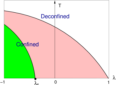
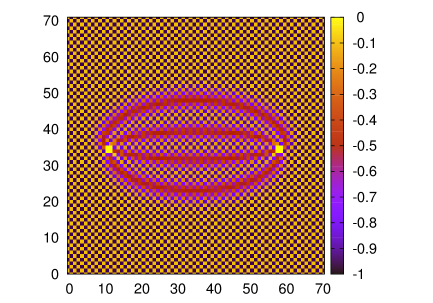
Figure 2: Left: a) Schematic sketch of the $\lambda$-$T$ phase diagram. Right: b) Energy density $-J\langle U_{\Box}+U_{\Box}^{\dagger}\rangle$ in the presence of two charges $\pm 2$ for $\lambda=0$ and $T=0$.

At zero temperature, the model is confining for $\lambda<1$, while at finite temperature $T$ it has a deconfinement phase transition. At $\lambda_{c}$ there is a quantum phase transition which separates two confined phases with spontaneously broken translation symmetry. The phase at $\lambda<\lambda_{c}$ has, in addition, a spontaneously broken charge conjugation symmetry. The two phases are similar to the columnar and plaquette ordered valence bond solid phases in a quantum dimer model [4]. In fact, the quantum dimer model has the same Hamiltonian as the quantum link model, but replaces the usual Gauss law by a staggered background of static charges $\pm 1$. It turns out that the quantum phase transition masquerades as a deconfined quantum critical point, at which an approximate spontaneously broken global $SO(2)$ symmetry with an almost massless pseudo-Goldstone boson emerges dynamically [83]. However, since the Goldstone boson is not exactly massless, it cannot be interpreted as a dual photon, and the theory remains confining at the quantum phase transition, albeit with a rather small string tension. An unbreakable confining string has an energy proportional to its length, with the string tension being the proportionality factor. In the $(2+1)$-d $U(1)$ quantum link model, the confining strings display unusual features. As illustrated in Figure 2b, the strings connecting two external charges $\pm 2$ separate into four mutually repelling strands, which each carry fractional electric flux $\frac{1}{2}$. The interior of the strands consists of the bulk phase that is stable on the other side of the phase transition. For integer spin $S$ on each link, one expects a less exotic confining dynamics. Once the $(2+1)$-d $U(1)$ quantum link model is realized in ultracold matter experiments, its dynamics in real-time will become accessible to quantum simulation. Since the model can be efficiently simulated in Euclidean time, experimental realizations of quantum simulators can be bench-marked accurately. For sufficiently large $S$, and perhaps even for $S=\frac{1}{2}$, the $(3+1)$-d $U(1)$ quantum link model exists in a Coulomb phase [84], which is interpreted as a spin liquid in condensed matter parlance [2].

3 Quantum Simulators for Abelian Lattice Gauge Theories

In this section we discuss constructions of quantum simulators for dynamical Abelian gauge theories, with and without matter fields, using both digital and analog simulation concepts.

3.1 Digital Quantum Simulators for ${\mathbb{Z}}(2)$ and $U(1)$ Gauge Theories

A digital quantum simulator is a precisely controllable many-body system, which can be programmed to execute a prescribed sequence of quantum gate operations. The state of the simulated system is encoded as quantum information, and its dynamics is represented by a sequence of quantum gates, following a stroboscopic Trotter decomposition [21]. The feasibility of universal digital quantum simulation with trapped ions has been demonstrated with 6 qubits and up to 100 gate operations in [85], where multi-spin interactions have also been implemented. While trapped ions offer a large degree of control of complicated interactions, these systems are still limited to a relatively small number of qubits and are hence currently not easily scalable. Utilizing engineered dissipative processes, entangled 4-qubit states, representing a single plaquette of Kitaev’s toric code, have been quantum simulated with trapped ions [86]. The toric code is equivalent to a ${\mathbb{Z}}(2)$ quantum link model on a 2-d quadratic spatial lattice with the Hamiltonian

$$H=-J\sum_{\Box}U_{\Box}-G\sum_{x}V_{x},\quad V_{x}=\exp\left[i\pi\sum_{k}(S^{3}_{x,x+\hat{k}}-S^{3}_{x-\hat{k},x})\right],$$ (3.1)

As in the $(2+1)$-d $U(1)$ quantum link model, there is a spin $\frac{1}{2}$, $\vec{S}_{xy}$, on each link. However, the quantum link operator is now given by $U_{xy}=S_{xy}^{1}$, such that the plaquette term $U_{\Box}=S_{wx}^{1}S_{xy}^{1}S_{yz}^{1}S_{zw}^{1}$ is invariant under discrete ${\mathbb{Z}}(2)$ gauge transformations $\Omega_{x}=\pm 1$. The $G$-term with $G>0$ punishes violations of the ${\mathbb{Z}}(2)$ Gauss law $V_{x}|\Psi\rangle=|\Psi\rangle$.

Optical lattices arise from the interference of counter-propagating laser beams. The lattice can be 1-, 2-, or 3-dimensional, with about 100 lattice sites per direction, and with a lattice spacing of a fraction of a $\mu$m. The resulting periodic structure of light can be loaded with up to about $10^{5}$ atoms from an ultracold Bose-Einstein condensate, which then settle down in the corresponding potential wells. By varying the depth of the optical potential, one controls the tunneling rate of atoms between neighboring wells. In this way, the phase transition between a Mott insulator of localized bosonic atoms and a superfluid has been quantum simulated [32]. Using lasers one can excite atoms to high-lying Rydberg states. Rydberg atoms are large objects with strong long-range dipole-dipole interactions, which can give rise to collective interactions of several atoms. Rydberg atoms in an optical lattice with a large lattice spacing can be addressed individually by external lasers. A Rydberg gate allows to entangle a number of atoms with a single control atom [87]. This is the basis of theoretical constructions of digital quantum simulators for $U(1)$ quantum link models [88, 72], which use control atoms at lattice sites to ensure Gauss’ law, as well as at plaquette centers to facilitate the flip of electric flux loops wrapping around flippable plaquettes. The ensemble Rydberg atoms represent qubits that reside at the link centers. By optical pumping, one can engineer dissipation that leads the system into the ground state, e.g. at the Rokhsar-Kivelson point $\lambda=1$. By further adiabatic evolution, one can then reach the ground state at any desired point in parameter space, and investigate, e.g., the dynamics of confining strings or the nature of quantum phase transitions.

3.2 Analog Quantum Simulators for $U(1)$ Gauge Theories

In an analog quantum simulator the time evolution proceeds continuously, rather than through a discrete sequence of quantum gates. These devices are usually limited to simpler interactions, but they are more easily scalable to large system sizes. The first quantum simulator for a gauge theory was proposed in [62]. It addresses the physics of the $U(1)$ quantum link model with $S=\frac{1}{2}$ using ultracold atoms in an optical lattice. The quantum links are embodied by hard-core bosons placed on the link centers. Their ring-exchange plaquette term is induced by a Raman transition that couples the bosons to a “molecular” two particle state localized at the plaquette center.

Zohar and Reznik have constructed a quantum simulator for Wilson’s compact $U(1)$ pure gauge theory [64]. In order to represent the continuously varying complex phase of $U_{xy}\in U(1)$, which gives rise to an infinite-dimensional Hilbert space per link, they have proposed to place a Bose-Einstein condensate on each link. In collaboration with Cirac [68], they have simplified this construction by restricting the number of bosons per link to $2S$, which truncates the Wilson theory to a $U(1)$ quantum link model with just a $(2S+1)$-dimensional link Hilbert space. Compact $(3+1)$-d $U(1)$ gauge theory describes magnetic monopoles interacting with photons. When the monopoles condense, the theory is confining [89], and a quantum simulator can thus address the corresponding non-perturbative effects. The confined phase at strong coupling is separated from a weakly coupled Coulomb phase by a first order phase transition. In the Coulomb phase, the monopoles have a mass at the cut-off scale, and the continuum limit just describes free photons. As was argued in [84], a quantum link model with small $S$ is sufficient to reach the continuum limit, and there is no need to approach the Wilson theory by increasing $S$ any further.

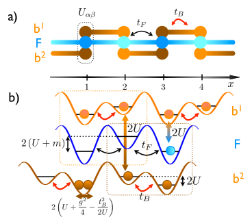
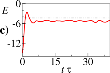
Figure 3: a) Quantum simulator of a $(1+1)$-d $U(1)$ quantum link model with fermionic matter using a Bose-Fermi mixture of cold atoms hopping in a 3-strand optical lattice. b) Mass $m$, hopping $t$, and interaction $U$ parameters are encoded in an optical superlattice. Energy conservation favors the simultaneous hopping of fermions and bosons, thus ensuring gauge invariance at low energies. c) Dynamical string breaking in real time $\tau$ (in units of the hopping parameter $t$): the string’s energy is converted into the mass of a dynamically created charge-anti-charge pair. In this process, the large negative electric flux $E$ of the string quickly relaxes to its vacuum value [69].

The physics becomes more interesting, and much more difficult to simulate on a classical computer, when dynamical fermions are added to the gauge field. Kapit and Mueller have proposed to use fermionic atoms hopping on a 2-d graphene-like optical honeycomb lattice, to engineer relativistic fermions at the corresponding Dirac cones [63]. In their construction, three bosonic species represent the components of the non-compact vector potential $A_{\mu}(x)$ of the $(2+1)$-d continuum theory. Since the theory was gauge-fixed in the continuum before it was discretized on a lattice, it is unclear whether, in this case, light gauge degrees of freedom emerge naturally.

In [69] a Bose-Fermi mixture was proposed to quantum simulate $U(1)$ quantum links, embodied by $2S$ bosons per link, coupled to dynamical staggered fermions. While the construction works in any dimension, it is particularly simple in 1-d, where it uses the 3-strand optical superlattice illustrated in Figure 3a. The Hamiltonian of eq.(2.15) (without the plaquette term) then arises in second order perturbation theory from a microscopic Hubbard-type Hamiltonian

$$\widetilde{H}=\sum_{x}h^{B}_{x,x+1}+\sum_{x}h^{F}_{x,x+1}+m\sum_{x}(-1)^{x}n_{x}^{F}+U\sum_{x}\widetilde{G}_{x}^{2},$$ (3.2)

which punishes gauge-variant states by a large energy penalty $U$. Here

$$\widetilde{G}_{x}=n_{x}^{F}+n^{B}_{x}-2S+\frac{1}{2}\left[(-1)^{x}-1\right],$$ (3.3)

is the infinitesimal generator of gauge transformations, with $n_{x}^{F}$ and $n^{B}_{x}$ counting the number of dynamical fermions and Schwinger bosons at the site $x$. The bosons that represent the $U(1)$ gauge field are confined to a given link, and just hop between the two ends $x$ and $x+1$ of that link, according to the hopping term $h^{B}_{x,x+1}=-t_{B}(b^{\dagger}_{x+1}b_{x}+b^{\dagger}_{x}b_{x+1})$. The number $b^{\dagger}_{x}b_{x}+b^{\dagger}_{x+1}b_{x+1}=2S$ of bosonic atoms is conserved locally on each link. In addition, one has spinless fermionic atoms at half-filling, which can hop between neighboring sites throughout the entire system, based on the hopping term $h^{F}_{x,x+1}=-t_{F}(\psi_{x+1}^{\dagger}\psi_{x}+\psi_{x}^{\dagger}\psi_{x+1})$. Due to the large energy penalty $U$, a fermion hopping from $x$ to $x+1$ is necessarily accompanied by a boson hopping the other way, thus ensuring gauge invariance in the low-energy sector by energy conservation (c.f. Figure 3b). This simple model can be used to study the dynamics of string breaking by charge-anti-charge pair creation in real time, a process which also arises in QCD. As illustrated schematically in Figure 4, an external static quark-anti-quark pair $\bar{Q}Q$ is connected by a confining electric flux string (Figure 4b), which manifests itself by a large value of the electric flux. For sufficiently small fermion mass, the potential energy stored in the string is converted into kinetic energy by fermion hopping, which amounts to the creation of a dynamical quark-anti-quark pair $q\bar{q}$ (Figures 4c,d). In the process of string breaking, an external static anti-quark $\bar{Q}$ pairs up with a dynamical quark to form a $\bar{Q}q$ meson (c.f. Figures 4e).

Figure 4: a) Half-filled vacuum of the $(1+1)$-d $U(1)$ quantum link model for $S=1$ with staggered fermions, b) string induced by a static external $\bar{Q}Q$ pair, c) broken string, d) evolution, e) final state with two mesons separated by vacuum. The dots denote sites occupied by a fermion and the double-arrows denote non-zero electric fluxes $E_{xy}=S_{xy}^{3}=-1$.

To illustrate what could be observed in a corresponding experiment, exact diagonalization results for the real-time evolution of the electric flux have been obtained for the quantum link model Hamiltonian with $S=1$. Figure 3c shows string breaking, starting from the initial state shown in Figure 4b. The large separation of the external static quark-anti-quark pair $\bar{Q}Q$ gives rise to a large energy stored in the confining string, which is then converted into the mass of two mesons. Indeed, the large negative electric flux initially stored in the string quickly approaches its vacuum value.

Quantum simulators for $U(1)$ gauge theories with fermionic matter have also been constructed in [71]. In [74] Zohar, Cirac, and Reznik made the interesting observation that $U(1)$ gauge invariance can be protected by angular momentum conservation in the interactions between the atoms representing fermions and gauge fields. Gauge invariance is then naturally maintained, once the initial state obeys the Gauss law.

4 Non-Abelian Gauge Theories

Non-Abelian gauge theories play a central role in the Standard Model of particle physics, which is a relativistic quantum field theory with the gauge group $SU(3)\times SU(2)_{L}\times U(1)_{Y}$. By the Higgs mechanism, the gauge symmetry gets broken to $SU(3)\times U(1)$, where $U(1)$ is the Abelian gauge group of electromagnetism and $SU(3)$ is the non-Abelian color gauge group controlling the strong interactions between quarks and gluons. Electromagnetism arises as a low-energy remnant of the electroweak symmetry $SU(2)_{L}\times U(1)_{Y}$, which governs the interactions of quarks, electrons, and neutrinos mediated by photons as well as massive W and Z bosons. While electromagnetism and the weak interactions can be understood in perturbation theory, the strong interactions require a non-perturbative treatment, at least at low energies. In particular, the QCD interaction between quarks and gluons is so strong that they do not exist as isolated particles, but are permanently confined inside protons, neutrons, and other hadrons. QCD can be regularized non-perturbatively on a lattice. In this framework, many important questions in particle physics are being addressed very successfully from first principles, using Monte Carlo simulations. Besides determining the hadron spectrum [90, 91, 92], which is vital for confirming QCD as the correct theory of the strong interactions also at low energies, lattice QCD calculations are important for the correct extraction of the quark masses by comparison with experiments. Furthermore, lattice QCD is vital for understanding the structure of hadrons and for investigating the physics of quarks and gluons at high temperatures [93, 94], which is explored in heavy ion collision experiments, e.g., at RHIC and at the LHC. Despite the many successes of lattice QCD, there are also significant challenges. Due to severe sign problems, dense systems of strongly interacting matter, such as the core of neutron stars, cannot be addressed with lattice QCD Monte Carlo simulations. For the same reason, the real-time evolution of strongly interacting systems remains beyond reach. These unsolved challenging problems are a strong motivation to formulate QCD as well as other non-Abelian gauge theories in a way that makes them accessible to atomic quantum simulation.

First, we discuss QCD in the continuum. In order to address non-perturbative effects, we then formulate the theory on the lattice, following Wilson. In order to ease the construction of quantum simulators, we also introduce non-Abelian quantum link models. We then present several quantum simulator constructions, and discuss potential experimental investigations.

4.1 Quantum Chromodynamics

Before we formulate QCD on the lattice, in this subsection we review some basic features of QCD in the continuum, using the manifestly relativistically invariant Lagrangian formulation. The QCD Lagrangian takes the form

$${\cal L}_{\text{QCD}}=\sum_{f,i}\overline{\psi}^{fi}(i\gamma^{\mu}D_{\mu ij}-m_{f})\psi^{fj}-\frac{1}{2g^{2}}\mbox{Tr}(G^{\mu\nu}G_{\mu\nu}).$$ (4.1)

The Dirac spinors $\psi^{fi}(x)$ and $\overline{\psi}^{fi}(x)={\psi^{fi}(x)}^{\dagger}\gamma^{0}$ describe quarks and anti-quarks of different flavors $f\in\{1,2,\dots,N_{f}\}$ and colors $i\in\{1,2,\dots,N\}$. The lightest quarks, which dominate ordinary matter, carry the flavors up and down. Protons consist of two u-quarks (each with electric charge $\frac{2}{3}e$) and one d-quark (of electric charge $-\frac{1}{3}e$), while neutrons consist of one u-quark and two d-quarks. In addition, protons and neutrons contain a fluctuating number of gluons and quark-anti-quark pairs. The non-Abelian vector potential, $G_{\mu}(x)=igG_{\mu}^{a}(x)T^{a}$, describing the gluons is constructed from real-valued fields $G_{\mu}^{a}(x)$ multiplying the $N^{2}-1$ traceless Hermitean generators $T^{a}$ of $SU(N)$ — the group of unitary $N\times N$ matrices with determinant 1. In the real world the number of colors is $N=3$. For $N=2$ the generators $T^{a}=\frac{1}{2}\sigma^{a}$ are given by the Pauli matrices, while for $N=3$ they are given by the Gell-Mann matrices $T^{a}=\frac{1}{2}\lambda^{a}$. Here $g$ is the strong coupling constant, i.e. the non-Abelian analog of the elementary electric charge $e$. The non-Abelian covariant derivative takes the form

$$D_{\mu}=\partial_{\mu}+G_{\mu}(x)\ \Rightarrow\ D_{\mu ij}=\partial_{\mu}\delta_{ij}+G_{\mu ij}(x)=\partial_{\mu}\delta_{ij}+igG_{\mu}^{a}(x)T_{ij}^{a},$$ (4.2)

and the gluon field strength tensor is given by

$$G_{\mu\nu}(x)=\partial_{\mu}G_{\nu}(x)-\partial_{\nu}G_{\mu}(x)+[G_{\mu}(x),G_{\nu}(x)].$$ (4.3)

Unlike photons, which are electrically neutral, gluons carry color charge. This manifests itself in the non-Abelian commutator term in $G_{\mu\nu}(x)$, which is absent in QED. The QCD Lagrangian is invariant under color gauge transformations $\Omega(x)\in SU(N)$ of the quark and gluon fields

$$\psi^{f}(x)^{\prime}=\Omega(x)\psi^{f}(x)\ \Rightarrow\psi^{fi}(x)^{\prime}=\Omega_{ij}(x)\psi^{fj}(x),$$

$$G_{\mu}(x)^{\prime}=\Omega(x)[G_{\mu}(x)+\partial_{\mu}]\Omega(x)^{\dagger}\ \Rightarrow\ G_{\mu\nu}(x)^{\prime}=\Omega(x)G_{\mu\nu}(x)\Omega(x)^{\dagger}.$$ (4.4)

It should be pointed out that, unlike $F_{\mu\nu}$ in Abelian gauge theories, the non-Abelian field strength $G_{\mu\nu}$ is not gauge invariant. The gluon field couples to the color index $i$ of the quark field $\psi^{fi}(x)$, but does not distinguish between quarks of different flavors $f$, which differ only in their masses $m_{f}$.

Quarks and anti-quarks are distinguished by their baryon numbers $B=\pm\frac{1}{N}$. In the real world (with $N=3$) three quarks form a baryon (e.g. a proton or neutron), while three anti-quarks from an anti-baryon (e.g. an anti-proton or anti-neutron). Under the global $U(1)_{B}$ baryon number symmetry the quark fields transform as $\psi^{fi}(x)^{\prime}=\exp(i\alpha)\psi^{fi}(x)$, which leaves ${\cal L}_{\text{QCD}}$ invariant. In the absence of quark masses, i.e. for $m_{f}=0$, the QCD Lagrangian has a global $SU(N_{f})_{L}\times SU(N_{f})_{R}$ chiral symmetry acting separately on the left- and right-handed quark and anti-quark fields. At low temperature, chiral symmetry is spontaneously broken to its vector subgroup $SU(N_{f})_{L=R}$, known as isospin for $N_{f}=2$. The order parameter for this symmetry breaking is the chiral condensate $\langle\overline{\psi}\psi\rangle=\langle 0|\sum_{f,i}\overline{\psi}^{f,i}(x)\psi^{f,i}(x)|0\rangle$. Here $|0\rangle$ is the QCD vacuum state, the lowest energy eigenstate in the sector with baryon number $B=0$. According to the Goldstone theorem, the spontaneous breakdown of chiral symmetry gives rise to $N_{f}^{2}-1$ Goldstone bosons — 3 pions in the $N_{f}=2$ case. In the real world, the masses $m_{u}$ and $m_{d}$ of the up and down quarks are small, but non-zero, which turns the pions into light, but not exactly massless, pseudo-Goldstone bosons. Besides the pions, the QCD spectrum contains other mesons (states with baryon number $B=0$ that contain an equal number of quarks and anti-quarks), as well as baryon resonances that decay into nucleons (protons or neutrons) and pions. Most important, the QCD spectrum does not contain states of isolated quarks or gluons, which are instead permanently confined inside hadrons.

4.2 Lattice QCD

The standard formulation of lattice QCD is due to Wilson. He represented the gluon field by parallel transporter $N\times N$ unitary matrices $U_{xy}$ of determinant 1, that take values in the non-Abelian color gauge group $SU(N)$, and are associated with the link connecting nearest neighbor lattice sites $x$ and $y$. While Wilson originally constructed the theory in the Lagrangian formulation, it was soon expressed by Kogut and Susskind in the Hamiltonian formulation [95]. In close analogy to lattice QED, again using staggered fermions, the lattice QCD Hamiltonian takes the form

$$H_{\text{QCD}} = -t\sum_{\langle xy\rangle}s_{xy}\left(\psi_{x}^{\dagger}U_{xy}\psi_{y}+\psi_{y}^{\dagger}U_{xy}^{\dagger}\psi_{x}\right)+m\sum_{x}s_{x}\psi_{x}^{\dagger}\psi_{x}$$ (4.5)

$$+ \frac{g^{2}}{2}\sum_{\langle xy\rangle}(L_{xy}^{2}+R_{xy}^{2})-\frac{1}{4g^{2}}\sum_{\Box}\mbox{Tr}\left(U_{\Box}+U_{\Box}^{\dagger}\right).$$

Here we are using one “flavor” of staggered fermions with mass $m$. Due to fermion doubling, in the continuum limit this will give rise to multiple fermion species. We have suppressed the color indices, which in a hopping term would appear as $\psi_{x}^{\dagger}U_{xy}\psi_{y}={\psi^{i}_{x}}^{\dagger}U^{ij}_{xy}\psi^{j}_{y}$. As in the Abelian case, the plaquette product $U_{\Box}=U_{wx}U_{xy}U_{zy}^{\dagger}U_{wz}^{\dagger}$ represents the color magnetic field. The color electric field is described by the flux operators $L_{xy}$ and $R_{xy}$, associated with the left and right end of the link $xy$. These non-Abelian analogs of $E_{xy}$ are operators that take appropriate derivatives with respect to the matrix elements of $U_{xy}$. Suppressing the link index $xy$, the various operators obey the commutation relations

$$[L^{a},L^{b}]=2if_{abc}L^{c},\quad[R^{a},R^{b}]=2if_{abc}R^{c},\quad[L^{a},R^{b}]=0,\quad[L^{a},U]=-\lambda^{a}U,\quad[R^{a},U]=U\lambda^{a}.$$ (4.6)

Operators associated with different links commute with each other. The Hermitean generators of $SU(N)$ obey the commutation relation $[\lambda^{a},\lambda^{b}]=2if_{abc}\lambda^{c}$, where $f_{abc}$ are the structure constants of the $SU(N)$ algebra and $\mbox{Tr}\lambda^{a}\lambda^{b}=2\delta^{ab}$. By construction, the Hamiltonian of eq.(4.5) is gauge invariant, i.e. it commutes with the infinitesimal generators of $SU(N)$ gauge transformations

$$G_{x}^{a}=\psi_{x}^{i\dagger}\lambda^{a}_{ij}\psi_{x}^{j}+\sum_{k}\left(L^{a}_{x,x+\hat{k}}+R^{a}_{x-\hat{k},x}\right),\quad[G^{a}_{x},G^{b}_{y}]=2i\delta_{xy}f_{abc}G^{c}_{x}.$$ (4.7)

Again, physical states $|\Psi\rangle$ are gauge invariant and must obey the Gauss law $G_{x}^{a}|\Psi\rangle=0$. A general $SU(N)$ gauge transformation, $\Omega_{x}=\exp(i\alpha_{x}^{a}\lambda^{a})$, is represented by the unitary transformation $V=\prod_{x}\exp(i\alpha_{x}^{a}G_{x}^{a})$, which acts as

$$\psi_{x}^{\prime}=V^{\dagger}\psi_{x}V=\Omega_{x}\psi_{x},\quad{\psi^{\dagger}_{x}}^{\prime}=V^{\dagger}\psi^{\dagger}_{x}V=\psi^{\dagger}_{x}\Omega_{x}^{\dagger},\quad U^{\prime}_{xy}=V^{\dagger}U_{xy}V=\Omega_{x}U_{xy}\Omega_{y}^{\dagger}.$$ (4.8)

In Wilson’s lattice gauge theory, the commutation relations of eq.(4.6) are realized in an infinite-dimensional Hilbert space per link. In fact, every link is analogous to a quantum mechanical “particle” moving in the group space $SU(N)$, with $L_{xy}^{2}+R_{xy}^{2}$ representing the corresponding Laplacian.

In an $SU(2)$ gauge theory the various operators can be represented by harmonic oscillators [96] (also known as prepotentials) using bosonic creation and annihilation operators $a^{i\dagger}_{x,\pm k}$ and $a^{i}_{x,\pm k}$, which carry a color index $i\in\{1,2\}$. The bosonic operators are associated with the left and right ends of a link and are labeled by a lattice point $x$ and a link direction $\pm k$, and one can write

$$L^{a}_{xy} = a^{i\dagger}_{x,+}\sigma^{a}_{ij}a^{j}_{x,+},\ R^{a}_{xy}=a^{i\dagger}_{y,-}\sigma^{a}_{ij}a^{j}_{y,-},$$

$$U_{xy} = \frac{1}{{\cal N}_{xy}}\left(\begin{array}[]{cc}a^{2\dagger}_{x,+}&a^{1}_{x,+}\\ -a^{1\dagger}_{x,+}&a^{2}_{x,+}\end{array}\right)\left(\begin{array}[]{cc}a^{1\dagger}_{y,-}&a^{2\dagger}_{y,-}\\ a^{2}_{y,-}&-a^{1}_{y,-}\end{array}\right)$$ (4.13)

$$= \frac{1}{{\cal N}_{xy}}\left(\begin{array}[]{cc}a^{2\dagger}_{x,+}a^{1\dagger}_{y,-}+a^{1}_{x,+}a^{2}_{y,-}&a^{2\dagger}_{x,+}a^{2\dagger}_{y,-}-a^{1}_{x,+}a^{1}_{y,-}\\ -a^{1\dagger}_{x,+}a^{1\dagger}_{y,-}+a^{2}_{x,+}a^{2}_{y,-}&-a^{1\dagger}_{x,+}a^{2\dagger}_{y,-}-a^{2}_{x,+}a^{1}_{y,-}\end{array}\right).$$ (4.16)

Here ${\cal N}_{xy}=a^{i\dagger}_{x,+}a^{i}_{x,+}=a^{i\dagger}_{y,-}a^{i}_{y,-}$ counts the number of bosons, which is the same at both ends of the link. The link operator $U_{xy}$ changes the number of bosons by two, by either creating or annihilating a boson on each end of a link. Since the link Hilbert space is infinite-dimensional, the total number of bosons can be arbitrarily large. In $SU(3)$ gauge theory the construction is much more involved [97]. Instead of two, it involves four species of colored bosons per link, which span a Hilbert space that is larger than the one of the gauge theory. In order to correct for this, the link operators are no longer constructed as boson bilinears, but as polynomials of a higher degree. Even then, the commutation relations of eq.(4.6) are satisfied only in the gauge theory subspace of the bosonic Hilbert space, and it is not obvious how to restrict oneself to that subspace. While there are constructions for quantum simulators using $SU(2)$ prepotentials [73, 74], it is difficult to imagine that the $SU(3)$ prepotentials of [97] can be implemented in ultracold matter.

Up to now, we have defined the theory on a lattice with non-zero lattice spacing $a$, whose inverse $\frac{1}{a}$ serves as an ultraviolet momentum cut-off. Ultimately, we want to take the continuum limit $a\rightarrow 0$. This is done by properly adjusting the bare coupling constant $g$. We may fix the overall energy scale by putting $t=1$. When we set $m=0$, we are in the chiral limit of massless quarks, which will lead to a massless Goldstone pion. The bare gauge coupling $g$ is then adjusted in order to take the continuum limit. This can be done by considering any dimensionful physical quantity, for example, the nucleon mass. The nucleon mass $M_{n}=E_{1}-E_{0}$ is the energy difference between the ground states of $H_{\text{QCD}}$ in the baryon number 1 and 0 sectors. Let us consider the nucleon mass in lattice units, i.e. $M_{n}a$, as a function of $g$. Due to the property of asymptotic freedom, in the $g\rightarrow 0$ limit the nucleon mass behaves as $M_{n}a\sim\exp(-\beta_{0}/g^{2})$, where $\beta_{0}>0$ is the leading coefficient of the QCD $\beta$-function. Keeping the physical quantity $M_{n}$ fixed and sending $g\rightarrow 0$, one approaches the continuum limit $a\rightarrow 0$. We have thus traded the dimensionless bare coupling constant $g$ for a dimensionful physical scale — in this case $M_{n}$. In this process of dimensional transmutation, the scale invariance of the QCD Lagrangian in the massless chiral limit is explicitly broken by the ultraviolet regulator $\frac{1}{a}$. It should be pointed out that massless QCD does not predict the value of any dimensionful scale like the nucleon mass. After all, the nucleon mass, e.g. in units of kilograms, relies on a man-made convention, and essentially reduces to the question how many protons and neutrons were deposited near Paris, when the kilogram was defined a long time ago. However, once an overall energy scale, e.g. $M_{n}$, has been picked, QCD predicts the values of countless dimensionless ratios, including the masses of nuclei $M_{B}=E_{B}-E_{0}$ in units of $M_{n}$. Here $E_{B}$ is the energy of the ground state in the sector with baryon number $B$, for example, the deuteron bound state of a proton and a neutron for $B=2$.

QCD gives rise to rich dynamics both at non-zero temperature and at non-zero baryon density. While chiral symmetry is spontaneously broken at low temperatures, it is restored at the high temperatures that existed in the early universe, and that are recreated in heavy-ion collisions. The crossover that separates the low- from the high-temperature phase has been accurately investigated using Monte Carlo simulations of lattice QCD [93, 94]. The QCD physics of non-zero baryon number, which governs individual nuclei as well as the matter deep inside neutron stars, is much less well understood from first principles. This is because Monte Carlo simulations fail at non-zero baryon density, due to a very severe sign problem. The same is true for studies of the real-time evolution, e.g. of a heavy-ion collision. These dynamics as well as the phases of matter at high baryon densities, which may include color superconductors [60, 61] (with or without color-flavor locking) provide a strong motivation to construct quantum simulators for non-Abelian gauge theories.

4.3 Non-Abelian Quantum Link Models

In contrast to Wilson’s lattice gauge theory, in quantum link models the real and imaginary parts of $U_{xy}^{ij}$ are no longer real numbers, but non-commuting Hermitean operators. The commutation relations of eq.(4.6) are then realized by using the generators of an $SU(2N)$ algebra. The real and imaginary parts of the $N^{2}$ matrix elements $U_{xy}^{ij}$ are represented by $2N^{2}$ Hermitean generators of the embedding algebra $SU(2N)$. The $2(N^{2}-1)$ generators $L^{a}_{xy}$ and $R^{a}_{xy}$ of $SU(N)$ gauge transformations at the left and at the right end of the link also belong to the $SU(2N)$ algebra. An additional Abelian $U(1)$ gauge transformation (which does not distinguish between left and right) is related to the generator $E_{xy}$. Altogether there are $2N^{2}+2(N^{2}-1)+1=4N^{2}-1$ generators, which form the embedding algebra $SU(2N)$. Similar constructions exist for $SO(N)$ and $Sp(N)$ gauge theories, which are naturally represented with $SO(2N)$ and $Sp(2N)$ embedding algebras [79]. Unlike in Wilson’s lattice gauge theory, where the different elements of a link matrix commute with each other as well as with their complex conjugates, i.e. $[U^{ij},U^{kl\dagger}]=0$, the elements of a quantum link matrix, $U^{ij}$, are non-commuting operators that obey the commutation relations

$$[U^{ij},U^{kl\dagger}]=2(\delta_{ik}\sigma^{a*}_{jl}R^{a}-\delta_{jl}\sigma^{a}_{ik}L^{a}+2\delta_{ik}\delta_{jl}E),\quad[U^{ij},U^{kl}]=[U^{ij\dagger},U^{kl\dagger}]=0.$$ (4.17)

Again, commutators between operators assigned to different links are zero. All other relations of Wilson’s QCD, including the Hamiltonian of eq.(4.5) and the gauge transformations of eqs.(4.7) and (4.8), remain valid in quantum link modes. The advantage of this alternative formulation of non-Abelian gauge theories is again that the Hilbert space is now finite-dimensional. Just as we could pick any value of the quantum spin $S$ in the Abelian $U(1)$ quantum link model (with the embedding algebra $SU(2)$), in the non-Abelian $SU(N)$ quantum link model we can pick any representation of the embedding algebra $SU(2N)$. In the appropriate limit of a large representation, one recovers the Wilson theory [98]. However, quantum link models are more than just a gauge invariant truncation of the Wilson theory. Indeed, they provide a non-trivial generalization of the concept of lattice gauge theories, with ample room for interesting new physical phenomena at strong coupling. As we have seen explicitly for the $(2+1)$-d $U(1)$ quantum link model, this also provides interesting connections to condensed matter physics.

It turns out that, in addition to the non-Abelian $SU(N)$ gauge invariance, the Hamiltonian of eq.(4.5) also has an Abelian $U(1)$ gauge symmetry which is generated by

$$G_{x}=\psi_{x}^{i\dagger}\psi_{x}^{i}+\sum_{k}\left(E_{x,x+\hat{k}}-E_{x-\hat{k},x}\right),\ [G_{x},G_{x}^{a}]=0.$$ (4.18)

If one wants to construct an $SU(N)$ rather than a $U(N)$ gauge theory, one should explicitly break the additional $U(1)$ symmetry. This can be done by adding the term $\gamma\sum_{\langle xy\rangle}\left(\mathrm{det}U_{xy}+\mathrm{det}U_{xy}^{\dagger}\right)$ to the Hamiltonian. Since all matrix elements $U^{ij}_{xy}$ commute with each other (although $U^{ij}_{xy}$ and $U^{kl\dagger}_{xy}$ do not commute) the definition of $\mbox{det}U_{xy}$ does not suffer from operator ordering ambiguities.

The commutation relations of eqs.(4.6) and (4.17) can be realized using fermionic rishons, representing constituents of gauge bosons. The rishon operators $c^{i}_{x,\pm k}$, $c^{i\dagger}_{x,\pm k}$ with color index $i\in\{1,2,\dots,N\}$ lead to the representation

$$L^{a}_{xy}=c^{i\dagger}_{x,+}\lambda^{a}_{ij}c^{j}_{x,+},\ R^{a}_{xy}=c^{i\dagger}_{y,-}\lambda^{a}_{ij}c^{j}_{y,-},\ E_{xy}=\frac{1}{2}(c^{i\dagger}_{y,-}c^{i}_{y,-}-c^{i\dagger}_{x,+}c^{i}_{x,+}),\ U^{ij}_{xy}=c^{i}_{x,+}c^{j\dagger}_{y,-}.$$ (4.19)

Rishon operators are associated with the left and right ends of a link and are labeled with a lattice point $x$ and a link direction $\pm k$. They obey canonical anti-commutation relations

$$\{c^{i}_{x,\pm k},c^{j\dagger}_{y,\pm l}\}=\delta_{xy}\delta_{\pm k,\pm l}\delta_{ij},\ \{c^{i}_{x,\pm k},c^{j}_{y,\pm l}\}=\{c^{i\dagger}_{x,\pm k},c^{j\dagger}_{y,\pm l}\}=0.$$ (4.20)

Quark and rishon operators also anti-commute with each other. All operators introduced so far (including the Hamiltonian) commute with the rishon number operator ${\cal N}_{xy}=c^{i\dagger}_{x,+}c^{i}_{x,+}+c^{i\dagger}_{y,-}c^{i}_{y,-}$ on each individual link. Hence, we can limit ourselves to sectors of fixed rishon number for each link. This is equivalent to working in a given irreducible representation of $SU(2N)$. We can write the determinant operator that we used to break the $U(N)$ gauge symmetry down to $SU(N)$ as

$$\mbox{det}U_{xy}=\frac{1}{N!}\epsilon_{i_{1}i_{2}...i_{N}}U_{xy}^{i_{1}i^{\prime}_{1}}U_{xy}^{i_{2}i^{\prime}_{2}}\dots U_{xy}^{i_{N}i^{\prime}_{N}}\epsilon_{i^{\prime}_{1}i^{\prime}_{2}\dots i^{\prime}_{N}}=N!\ c^{1}_{x,+}c^{1\dagger}_{y,-}c^{2}_{x,+}c^{2\dagger}_{y,-}\dots c^{N}_{x,+}c^{N\dagger}_{y,-}.$$ (4.21)

Only when this operator acts on a state with exactly ${\cal N}=N$ rishons (all of a different color), it gives a non-zero contribution. In all other cases the determinant vanishes. This means that we can reduce the symmetry from $U(N)$ to $SU(N)$ via the determinant when we work with ${\cal N}=N$ fermionic rishons on each link. The number of fermion states per link then is $(2N)!/(N!)^{2}$. For an $SU(2)$ gauge theory the Hilbert space of the corresponding quantum link model then has 6 states per link, while for $SU(3)$ it has 20 states per link. In the standard Wilson formulation of lattice gauge theory, on the other hand, the single link Hilbert space is already infinite-dimensional. This limit can be recovered when one introduces a large number of rishon “flavors” [98]. The rishon dynamics are illustrated in Figure 5a.

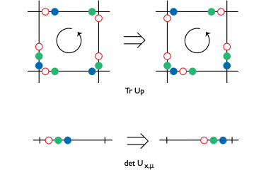
Figure 5: Left: a) In an $SU(3)$ quantum link model, three fermionic rishons of different colors reside on each link. The Hamiltonian moves the rishons around plaquettes or along links, like the beads of an abacus. Right: b) In the quantum link formulation of QCD, the size $\beta$ of an extra dimension is small compared to the gluonic and fermionic correlation lengths $1/m$ and $1/\mu$, and the theory undergoes dimensional reduction. Effective continuous gluon fields emerge from the discrete quantum link variables, and quark modes $\Psi_{L}$ and $\Psi_{R}$ appear as domain wall fermions.

In the D-theory formulation of quantum field theory, the continuum limit of quantum link models is approached by dimensional reduction from a higher dimension [77]. Since non-Abelian gauge theories in $(4+1)$-d have massless Coulomb phases, one naturally reaches the exponentially small masses of asymptotically free field theories by dimensional reduction. Effective continuous 4-d gluon fields then arise as collective excitations of discrete quantum link variables, just as effective magnon fields arise as collective excitations of quantum spins. Chiral quarks are incorporated naturally as domain wall fermions, which arise as massless 4-d edge-modes on a $(4+1)$-d slab, analogous to the edge-states of a quantum Hall sample (c.f. Figure 5b). Universality then implies that one recovers QCD in the continuum limit.

Quantum simulators will first be realized in the strong coupling regime, in which there is no need for large link Hilbert spaces or complicated plaquette interactions. Even if they do not yet represent Nature’s QCD, strongly coupled lattice gauge models already display rich dynamics including confinement and deconfinement, chiral symmetry breaking and restoration , and perhaps even color superconductivity. By quantum simulating such models, one may learn a lot about fundamental dynamical mechanisms in non-Abelian gauge theories, which will be very useful both in particle and in condensed matter physics.

5 Quantum Simulators for non-Abelian Lattice Gauge Theories

In this section, we discuss both digital and analog quantum simulators for non-Abelian gauge theories, again with and without matter fields.

5.1 Digital Quantum Simulator for an $SU(2)$ Gauge Theory

Because $SU(2)\simeq SO(3)$ is also equivalent to $Sp(1)$, it can be realized both in an $SU(4)\simeq SO(6)$ and in an $Sp(2)\simeq SO(5)$ embedding algebra. The quantum link model that was originally constructed by Horn is based on an $SO(5)$ embedding [75]. Orland and Rohrlich used the 4-state $SO(5)$ spinor representation in their study of the $(2+1)$-d gauge magnet [76]. A quantum simulator for this system, using Rydberg atoms in an optical lattice, has been proposed in [72]. It utilizes two ensemble atoms per link, in a holographically designed optical lattice [99, 100], which encode the 4 link states, as well as control atoms at the lattice sites and at the plaquette centers. These atoms control an eight-qubit interaction realizing the plaquette product $U_{\Box}$. Protocols for ground state preparation in the presence of external static charges, as well as methods for detecting the confining strings connecting the charges by direct imaging have also been proposed.

5.2 Analog Quantum Simulators for $U(N)$ and $SU(N)$ Gauge Theories

Analog quantum simulators for $SU(2)$ gauge theories coupled to fermionic matter, based on the bosonic prepotential representation of Wilson’s $SU(2)$ gauge theory [96] have been proposed in [73, 74] using a Fermi-Bose mixture of atoms in an optical superlattice. Four bosonic and one auxiliary fermionic species reside on each link, representing the “gluon” gauge field. In order to model the infinite-dimensional Hilbert space of the Wilson theory, two bosonic species form a Bose-Einstein condensate. The “quarks” are embodied by another species of fermionic atoms. Using higher-order processes, plaquette interactions have also been constructed in this way.

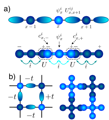
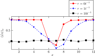
Figure 6: Left: Quantum simulator for an $SU(N)$ gauge theory with ultracold alkaline-earth atoms representing “quarks” or rishon constituents of “gluons” in a 1-d (a) or 2-d (b) optical superlattice. Right: c) Real-time $\tau$ evolution of the chiral order parameter profile $(\overline{\psi}\psi)_{x}$ in a $U(2)$ gauge theory, mimicking the expansion of a hot quark-gluon plasma [70].

An alternative proposal is based on the rishon formulation of $U(N)$ and $SU(N)$ quantum link models [70]. This construction uses fermionic alkaline-earth atoms [101, 102, 103], such as ${}^{87}Sr$ or ${}^{173}Yb$, hopping in an optical superlattice [104]. The interactions between the atoms can be engineered, e.g., using Feshbach resonances [105, 106]. The color degree of freedom is encoded in the Zeeman states of the nuclear spin $I$, which enjoy an $SU(2I+1)$ symmetry. Each link has two rishon-sites, one associated with each end of the link. The number of rishons, ${\cal N}_{xy}=c_{x,+k}^{i\dagger}c_{x,+k}^{i}+c_{y,-k}^{i\dagger}c_{y,-k}^{i}$, on each link is fixed to $n$, due to a Hubbard-type energy penalty

$$\widetilde{H}=\tilde{t}\sum_{x,k}\left(s_{xy}c^{i\dagger}_{x,+k}\psi^{i}_{x}+c^{i\dagger}_{x,-k}\psi^{i}_{x}+\mathrm{h.c.}\right)+m\sum_{x}s_{x}\psi_{x}^{i\dagger}\psi^{i}_{x}+U\sum_{\langle xy\rangle}(\mathcal{N}_{xy}-n)^{2}.$$ (5.1)

When an atom resides on a rishon-site $x,\pm k$ it embodies a fermionic constituent of a “gluon”. When the same atom hops to an ordinary lattice site $x$, it embodies a “quark”. $SU(N)$ gauge invariance is thus naturally protected by the dynamics, while the additional $U(1)$ gauge symmetry is explicitly violated at the cut-off scale, but emerges at low energy. Small explicit violations of the gauge symmetry are tolerable, because gauge invariance is robust at low energies [12, 107]. $U(N)$ gauge theories do not contain baryons, because $U(1)$ is gauged, and baryons are confined at strong coupling. $U(2)$ lattice gauge theories, which can be realized with a single rishon per link, are still interesting, e.g., because they have a spontaneously broken chiral symmetry, whose dynamics can be investigated in real time. Figure 6c shows the evolution of the profile of the chiral condensate $(\overline{\psi}\psi)_{x}$ (i.e. the order parameter for spontaneous chiral symmetry breaking), derived by exact diagonalization of a moderate-size 1-d system. The initial configuration contains a small region in which the order parameter deviates from its vacuum value, thus mimicking a hot quark-gluon plasma. As time evolves, this region expands. When ${\cal N}=N$ one can use the $\mbox{det}U$-term to reduce the gauge symmetry from $U(N)$ to $SU(N)$. For $SU(2)$ one then obtains bosonic “baryons”, whose quantum simulation requires simultaneous two-rishon tunneling, which can be implemented as a Raman process. In such a model, one can study chiral symmetry restoration at non-zero baryon density. Nature’s $SU(3)$ gauge symmetry yields fermionic baryons (e.g., protons and neutrons) which would require the engineering of a three-rishon tunneling process (c.f. Figure 5a, bottom), whose realization is more challenging.

6 Conclusions and Outlook

As we have seen, there are many exciting ideas how to quantum simulate dynamical lattice gauge theories, which are of interest both in particle and in condensed matter physics. When quantum link models or gauge magnets with plaquette interactions are used to model condensed matter systems, such as spin liquids, one can use digital simulations using Rydberg atoms in an optical lattice. It would also be very interesting to investigate whether $(2+1)$-d Chern-Simons gauge theories can be regularized with quantum link models. If so, one might be able to realize non-Abelian anyons with ultracold matter in optical lattices. This might enable topological quantum computation [6], which is robust against decoherence, with exquisite experimental control. Aiming at particle physics applications, one may pursue different strategies. When one uses the Wilson formulation with bosonic prepotentials, the continuous nature of Wilson’s parallel transporters, which results in an infinite-dimensional link Hilbert space, demands a large number of bosons per link, possibly forming a Bose-Einstein condensate. The continuum limit is then taken by tuning the plaquette coupling, which is non-trivial to engineer, to a large value (which corresponds to sending $g\rightarrow 0$). Plaquette couplings can also be induced with additional fermion flavors [108], or with scalar fields [109].

Quantum link models offer an alternative to this strategy. Thanks to the discrete nature of the quantum link variables, these models can be embodied by a few particles per link, thus benefiting from their low-dimensional link Hilbert space. Generically, quantum link models are lattice gauge theories at strong coupling, which often do not need plaquette interactions to display interesting dynamics. As such, they offer a unique opportunity to explore fundamental features of strong gauge dynamics with a minimal set of degrees of freedom. This includes investigations of confinement and deconfinement, chiral symmetry breaking and restoration at finite baryon density [110, 111], and perhaps even color superconductivity. Long before one ultimately takes the continuum limit, quantum simulating these intriguing phenomena with ultracold atomic gases would be most exciting, and indeed seems within reach in the foreseeable future.

Various types of Bose-Bose, Fermi-Fermi and Bose-Fermi mixtures are available in the laboratory. Different set-ups may be engineered within state of the art technologies [112], each of them highly tunable and characterized by efficient detection techniques such as in situ imaging, leading to precise snapshots of the particles’ spatial distribution. Ultracold gases of heteronuclear molecules offer even more tunable set-ups, since one can exploit the rich internal structure of such objects to properly design several types of interactions [113]. Rydberg atoms in optical lattices or alkaline-earth atoms offer further opportunities. While the realization of the proposed quantum simulators is challenging, and will require the combination of several existing experimental techniques, the ball is now in the court of the experimental colleagues, to utilize their rich arsenal of powerful experimental techniques, and to go ahead and quantum simulate dynamical gauge fields. Theorists should support this process, by further simplifying the existing constructions, wherever this seems possible. Experimentally, one probably wants to start with a simple case. A well-defined first goal could be to realize the $(1+1)$-d $U(1)$ quantum link model with fermionic matter, in order to study the real-time evolution of string breaking. Moving on to higher dimensions and to non-Abelian gauge theories are natural next steps.

An ultimate long-term goal will be to quantitatively address the QCD phase diagram at non-zero baryon density and the real-time evolution of heavy-ion collisions. This will require a correct implementation of chiral symmetry. In the quantum link model based D-theory formulation of QCD, this is naturally provided by domain wall fermions, which requires multi-component fermion fields for which further tools from atomic physics would have to be developed. In D-theory, the continuum limit of an asymptotically free gauge theory, such as QCD, is taken by the dimensional reduction of the discrete quantum link variables from an additional spatial dimension, with an extent of just a few lattice spacings. While it will be challenging to endow ultracold matter with something equivalent to an extra dimension, this seems not impossible. In particular, one can imagine encoding the discrete coordinate of the extra dimension in an internal atomic state or realize it with distinct atomic species. Recovering Lorentz invariance will happen almost automatically in the D-theory set-up, except that the “velocity of light” of the quarks must be tuned to match the one of the gluons. While quantum simulating QCD near the continuum limit may remain a very long-term goal, there is a lot of exciting physics to be discovered along the way.

References

- [1] M. Levin, X. Wen, Rev. Mod. Phys. 77 (2005) 871.
- [2] M. Hermele, M. P. A. Fisher, L. Balents, Phys. Rev. B69 (2004) 064404.
- [3] D. S. Rokhsar, S. A. Kivelson, Phys. Rev. Lett. 61 (1988) 2376.
- [4] R. Moessner, S. L. Sondhi, E. Fradkin, Phys. Rev. B65 (2002) 024504.
- [5] A. Y. Kitaev, Ann. Phys. 303 (2003) 2.
- [6] C. Nayak, S. H. Simon, A. Stern, M. Freedman, S. Das Sarma, Rev. Mod. Phys. 80 (2008) 1083.
- [7] C. N. Yang, R. Mills, Phys. Rev. D96 (1954) 191.
- [8] G. ’t Hooft, M. J. G. Veltman, Nucl. Phys. B44 (1972) 189.
- [9] D. Gross, F. Wilczek, Phys. Rev. Lett. 30 (1973) 1343.
- [10] D. Politzer, Phys. Rev. Lett. 30 (1973) 1346.
- [11] H. Fritzsch, M. Gell-Mann, H. Leutwyler, Phys. Lett. B47 (1973) 365.
- [12] D. Foerster, H. Nielsen, M. Ninomiya, Phys. Lett. B94 (1980) 135.
- [13] T. Sentil, A. Vishwanath, L. Balents, S. Sachdev, M. P. A. Fisher, Science 303 (2004) 1490.
- [14] M. Troyer, U.-J. Wiese, Phys. Rev. Lett. 94 (2005) 170201.
- [15] M. H. Anderson, J. R. Ensher, M. R. Matthews, C. E. Wieman, E. A. Cornell, Science 269 (1995) 5221.
- [16] K. B. Davis, M. O. Mewes, M. R. Andrews, N. J. van Druten, D. S. Durfee, D. M. Kurn, W. Ketterle, Phys. Rev. Lett. 75 (1995) 3969.
- [17] P. W. Shor, SIAM J. Sci. Statist. Comput. 26 (1997) 1484.
- [18] J. I. Cirac, P. Zoller, Phys. Rev. Lett. 74 (1995) 4091.
- [19] R. P. Feynman, Int. J. Theor. Phys. 21 (1982) 467.
- [20] J. I. Cirac, P. Zoller, Nat. Phys. 8 (2012) 264.
- [21] S. Lloyd, Science 273 (1996) 1073.
- [22] D. Jaksch, C. Bruder, J. I. Cirac, C. W. Gardiner, P. Zoller, Phys. Rev. Lett. 81 (1998) 3108.
- [23] M. Lewenstein, A. Sanpera, V. Ahufinger, “Ultracold Atoms in Optical Lattices: Simulating Quantum Many-Body Systems”, Oxford University Press (2012).
- [24] I. Bloch, J. Dalibard, S. Nascimbene, Nat. Phys. 8 (2012) 267.
- [25] R. Blatt, C. F. Ross, Nat. Phys. 8 (2012) 277.
- [26] A. Aspuru-Guzik, P. Walther. Nat. Phys. 8 (2012) 285
- [27] A. A. Houck, H. E. Türeci, J. Koch. Nat. Phys. 8 (2012) 292.
- [28] E. Farhi, J. Goldstone, S. Gutmann, M. Sipser, arXiv:0001106.
- [29] S. Boixo, T. F. Ronnow, S. V. Isakov, Z. Wang, D. Wecker, D. A. Lidar, J. M. Martinis, M. Troyer, arXiv:1304.4595.
- [30] L. Duan, E. Demler, M. Lukin, Phys. Rev. Lett. 91 (2003) 90402.
- [31] P. A. Lee, N. Nagaosa, X. G. Wen, Rev. Mod. Phys. 78 (2006) 17.
- [32] M. Greiner, O. Mandel, T. Esslinger, T. W. Hänsch, I. Bloch, Nature 415 (2002) 39.
- [33] S. Trotzky, L. Pollet, F. Gerbier, U. Schnorrberger, I. Bloch, N. Prokovéf, B. Svistunov, M. Troyer, Nat. Phys. 6 (2010) 998.
- [34] A. Retzker, J. I. Cirac, B. Reznik, Phys. Rev. Lett. 94 (2005) 050504.
- [35] B. Horstmann, B. Reznik, S. Fagnocchi, J. I. Cirac, Phys. Rev. Lett. 104 (2010) 250403.
- [36] S. P. Jordan, K. S. Lee, J. Preskill, Science 336 (2012) 1130.
- [37] J. I. Cirac, P. Maraner, J. K. Pachos, Phys. Rev. Lett. 105 (2010) 190403.
- [38] A. Bermudez, L. Mazza, M. Rizzi, N. Goldman, M. Lewenstein, M. A. Martin-Delgado, Phys. Rev. Lett. 105 (2010) 190404.
- [39] O. Boada, A. Celi, J. I. Latorre, M. Lewenstein, N. J. of Phys. 13 (2011) 035002.
- [40] L. Mazza, A. Bermudez, N. Goldman, M. Rizzi, M. A. Martin-Delgado, M. Lewenstein, N. J. of Phys. 14 (2012) 015007.
- [41] D. Jaksch, P. Zoller, New J. Phys. 5 (2003) 56.
- [42] K. Osterloh, M. Baig, L. Santos, P. Zoller, M. Lewenstein, Phys. Rev. Lett. 95 (2005) 010403.
- [43] J. Ruseckas, G. Juzeliunas, P. Öhberg, M. Fleischhauer, Phys. Rev. Lett. 95 (2005) 010404.
- [44] N. Goldman, A. Kubasiak, A. Bermudez, P. Gaspard, M. Lewenstein, M. Martin-Delgado, Phys. Rev. Lett. 103 (2009) 035301.
- [45] Y.-J. Lin, R. L. Compton, K. Jimenez-Garcia, J. V. Porto, I. B. Spielman, Nature 462 (2009) 628.
- [46] Y.-J. Lin, K. Jimenez-Garcia, I. B. Spielman, Nature 471 (2011) 83.
- [47] N. Cooper, Phys. Rev. 106 (2011) 175301.
- [48] M. Adelsburger, M. Atala, S. Nascimbene, S. Trotsky, Y.-A. Chen, I. Bloch, Phys. Rev. Lett. 107 (2011) 255301.
- [49] J. Dalibard, F. Gerbier, G. Juzeliunas, P. Öhberg, Rev. Mod. Phys. 83 (2011) 1523.
- [50] M. J. Edmonds, M. Valiente, G. Juzeliunas, L. Santos, P. Öhberg, Phys. Rev. Lett. 110 (2013) 085301.
- [51] K. G. Wilson, Phys. Rev. D10 (1974) 2445.
- [52] J. Kogut, Rev. Mod. Phys. 51 (1979) 659.
- [53] J. Kogut, Rev. Mod. Phys. 55 (1983) 775.
- [54] M. Creutz, “Quarks, Gluons, and Lattices”, Cambridge University Press (1985).
- [55] I. Montvay, G. Münster, “Quantum Fields on a Lattice”, Cambridge University Press (1994).
- [56] T. DeGrand, C. DeTar, “Lattice Methods for Quantum Chromodynamics”, World Scientific (2006).
- [57] C. Gattringer, C. Lang, “Quantum Chromodynamics on the Lattice: An Introductory Presentation”, Lecture Notes in Physics, Springer (2010).
- [58] D. H. Rischke, Prog. Part. Nucl. Phys. 52 (2004) 197.
- [59] K. Fukushima, T. Hatsuda, Rept. Prog. Phys. 74 (2011) 014001.
- [60] K. Rajagopal, F. Wilczek, in “At the Frontier of Particle Physics”, ed. M. Shifman (2000).
- [61] M. G. Alford, A. Schmitt, K. Rajagopal, T. Schäfer, Rev. Mod. Phys. 80 (2008) 1455.
- [62] H. P. Büchler, M. Hermele, S. D. Huber, M. P. A. Fisher, P. Zoller, Phys. Rev. Lett. 95 (2005) 040402.
- [63] E. Kapit, E. Mueller, Phys. Rev. A83 (2011) 033625.
- [64] E. Zohar, B. Reznik, Phys. Rev. Lett. 107 (2011) 275301.
- [65] G. Szirmai, E. Szirmai, A. Zamora, M. Lewenstein, Phys. Rev. A84 (2011) 011611.
- [66] Y. Liu, Y. Meurice, S.-W. Tsai, arXiv:1211.4126
- [67] L. Tagliacozzo, A. Celi, P. Orland, M. Lewenstein, arXiv:1211.2704 (2012).
- [68] E. Zohar, J. Cirac, B. Reznik, Phys. Rev. Lett. 109 (2012) 125302.
- [69] D. Banerjee, M. Dalmote, M. Müller, E. Rico, P. Stebler, U.-J.. Wiese, P. Zoller, Phys. Rev. Lett. 109 (2012) 175302.
- [70] D. Banerjee, M. Bögli, M. Dalmote, E. Rico, P. Stebler, U.-J.. Wiese, P. Zoller, Phys. Rev. Lett. 110 (2013) 125303.
- [71] E. Zohar, J. Cirac, B. Reznik, Phys. Rev. Lett. 110 (2013) 055302.
- [72] L. Tagliacozzo, A. Celi, A. Zamora, M. Lewenstein, Ann. Phys. 330 (2013) 160.
- [73] E. Zohar, J. Cirac, B. Reznik, Phys. Rev. Lett. 110 (2013) 125304.
- [74] E. Zohar, J. Cirac, B. Reznik, arXiv:1303.5040.
- [75] D. Horn, Phys. Lett. B100 (1981) 149.
- [76] P. Orland, D. Rohrlich, Nucl. Phys. B338 (1990) 647.
- [77] S. Chandrasekharan, U.-J. Wiese, Nucl. Phys. B492 (1997) 455.
- [78] R. C. Brower, S. Chandrasekharan, U.-J. Wiese, Phys. Rev. D60 (1999) 094502.
- [79] R. C. Brower, S. Chandrasekharan, S. Riederer, U.-J. Wiese, Nucl. Phys. B693 (2004) 149.
- [80] H. B. Nielsen, M. Ninomiya, Nucl. Phys. B185 (1981) 20.
- [81] D. B. Kaplan, Phys. Lett. B288 (1992) 342.
- [82] L. Susskind, Phys. Rev. D16 (1977) 3031.
- [83] D. Banerjee, F.-J. Jiang, P. Widmer, U.-J. Wiese, arXiv:1303.6858.
- [84] S. Chandrasekharan, Nucl. Phys. Proc. Suppl. 73 (1999) 739.
- [85] B. P. Lanyon, C. Hempel, D. Nigg, M. Müller, R. Gerritsma, F. Zähringer, P. Schindler, J. T. Barreiro, M. Rambach, G. Kirchmair, M. Hennrich, P. Zoller, R. Blatt, C. F. Roos, Science 334 (2011) 6052.
- [86] J. T. Barreiro, M. Müller, P. Schindler, D. Nigg, T. Monz, M. Chwalla, M. Hennrich, C. F. Roos, P. Zoller, R. Blatt, Nature 470 (2011) 486.
- [87] M. Müller, I. Lesanovsky, H. Weimer, H. P. Büchler, P. Zoller, Phys. Rev. Lett. 102 (2009) 170502.
- [88] H. Weimer, M. Müller, I. Lesanovsky, P. Zoller, H. P. Büchler, Nat. Phys. 6 (2010) 382.
- [89] A. M. Polyakov, Nucl. Phys. B120 (1977) 429.
- [90] S. Dürr, Z. Fodor, J. Frison, C. Hoelbling, R. Hoffmann, S. D. Katz, S. Krieg, T. Kurth, L. Lellouch, T. Lippert, K. K. Szabo, G. Vulvert, Science 322 (2008) 1224.
- [91] MILC collaboration, A. Bazavov et al., Rev. Mod. Phys. 82 (2010) 1349.
- [92] RBC and UKQCD collaborations, Y. Aoki et al., Phys. Rev. D83 (2011) 074508.
- [93] Y. Aoki, G. Endrodi, Z. Fodor, S. D. Katz, K. K. Szabo, Nature 443 (2006) 675.
- [94] MILC collaboration, A. Bazavov et al., Phys.Rev. D80 (2009) 014504.
- [95] J. Kogut, L. Susskind, Phys. Rev. D11 (1975) 395.
- [96] M. Mathur, J. Phys. A38 (2005) 10015.
- [97] R. Anishetty, M. Mathur, I. Raychowdhury, J. Phys. A43 (2010) 035403.
- [98] B. Schlittgen, U.-J. Wiese, Phys. Rev. D63 (2001) 085007.
- [99] W. S. Bakr, J. I. Gillen, A. Peng, S. Fölling, M. Greiner, Nature 462 (2009) 74.
- [100] C. Weitenberg, M. Endres, J. F. Sherson, M. Cheneau, P. Schauss, T. Fukuhara, I. Bloch, S. Kuhr, Nature 471 (2011) 319.
- [101] M. A. Cazalilla, A. F. Ho, M. Ueda, New J. Phys. 11 (2009) 103033.
- [102] A. V. Gorshkov, M. Hermele, V. Gurarie, C. Xu, P. S. Julienne, J. Ye, P. Zoller, E. Demler, M. D. Lukin, A. M. Rey, Nat. Phys. 6 (2010) 289.
- [103] S. Taie, R. Yamazaki, S. Sugawa, Y. Takahashi, Nat. Phys. 8 (2012) 825.
- [104] A. J. Dalley, M. M. Boyd, J. Ye, P. Zoller, Phys. Rev. Lett. 101 (2008) 170504.
- [105] R. Ciurylo, E. Tiesinga, P. S. Julienne, Phys. Rev. A71 (2005) 030701.
- [106] C. Chin, R. Grimm, P. S. Julienne, E. Tiesinga, Rev. Mod. Phys. 82 (2010) 1225.
- [107] K. Kasamatsu, I. Ichinose, T. Matsui, arXiv:1212.4952.
- [108] A. Hasenfratz, P. Hasenfratz, Phys. Lett. B297 (1992) 166.
- [109] C. Wetterich, arXiv:1212.3507.
- [110] S. Chandrasekharan, F.-J. Jiang, Phys. Rev. D74 (2006) 014506.
- [111] S. Chandrasekharan, A. Li, JHEP 1012 (2010) 021.
- [112] I. Bloch, J. Dalibard, W. Zwerger, Rev. Mod. Phys. 80 (2008) 885.
- [113] T. Lahaye, C. Menotti, L. Santos, M. Lewenstein, T. Pfau, Rep. Prog. Phys. 72 (2009) 126401.