Stein structures: existence and flexibility

Abstract.

This survey on the topology of Stein manifolds is an extract from the book [7]. It is compiled from two short lecture series given by the first author in 2012 at the Institute for Advanced Study, Princeton, and the Alfréd Rényi Institute of Mathematics, Budapest.

1. The topology of Stein manifolds

Throughout this article, $(V,J)$ denotes a smooth manifold (without boundary) of real dimension $2n$ equipped with an almost complex structure $J$, i.e., an endomorphism $J:TV\to TV$ satisfying $J^{2}=-{\rm id}$. The pair $(V,J)$ is called an almost complex manifold. It is called a complex manifold if the almost complex structure $J$ is integrable, i.e., $J$ is induced by complex coordinates on $V$. By the theorem of Newlander and Nirenberg [24], a (sufficiently smooth) almost complex structure $J$ is integrable if and only if its Nijenhuis tensor

$$N(X,Y):=[JX,JY]-[X,Y]-J[X,JY]-J[JX,Y],\qquad X,Y\in TV,$$

vanishes identically. An integrable almost complex structure is called a complex structure.

A complex manifold $(V,J)$ is called Stein if it admits a proper holomorphic embedding into some ${\mathbb{C}}^{N}$. Note that, due to the maximum principle, every Stein manifold is open, i.e., it has no compact components.

By a theorem of Grauert, Bishop and Narasimhan [13, 2, 23], a complex manifold $(V,J)$ is Stein if and only if it admits a smooth function $\phi:V\to{\mathbb{R}}$ which is

• exhausting, i.e., proper and bounded from below, and

• $J$-convex (or strictly plurisubharmonic), i.e., $-dd^{\mathbb{C}}\phi(v,Jv)>0$ for all $0\neq v\in TV$, where $d^{\mathbb{C}}\phi:=d\phi\circ J$.

Note that the second condition means that $\omega_{\phi}:=-dd^{\mathbb{C}}\phi$ is a symplectic form compatible with $J$. Note also that the “only if” follows simply by restricting the $i$-convex function $\phi(z)=|z|^{2}$ on ${\mathbb{C}}^{N}$ (where $i$ denotes the standard complex structure) to a properly embedded complex submanifold. Here are some examples of Stein manifolds.

(1) $({\mathbb{C}}^{n},i)$ is Stein, and properly embedded complex submanifolds of Stein manifolds are Stein.

(2) If $X$ is a closed complex submanifold of some projective space ${\mathbb{C}}P^{N}$ and $H\subset{\mathbb{C}}P^{N}$ is a hyperplane, then $X\setminus H$ is Stein.

(3) All open Riemann surfaces are Stein.

(4) If $\phi:V\to{\mathbb{R}}$ is $J$-convex, then so is $f\circ\phi$ for any smooth function $f:{\mathbb{R}}\to{\mathbb{R}}$ with $f^{\prime}>0$ and $f^{\prime\prime}\geq 0$ (such $f$ will be called a convex increasing function). Given an exhausting $J$-convex function $\phi:V\to{\mathbb{R}}$ and any $c\in{\mathbb{R}}$, we can pick a diffeomorphism $f:(-\infty,c)\to{\mathbb{R}}$ with $f^{\prime}>0$ and $f^{\prime\prime}\geq 0$; then $f\circ\phi$ is an exhausting $J$-convex function $\{\phi<c\}\to{\mathbb{R}}$, hence the sublevel set $\{\phi<c\}$ is Stein.

(5) Any strictly convex smooth function $\phi:{\mathbb{C}}^{n}\to{\mathbb{R}}$ is $i$-convex. As a consequence, using (4), all convex open subsets of ${\mathbb{C}}^{n}$ are Stein.

(6) Let $L\subset V$ be a properly embedded totally real submanifold, i.e., $L$ has real dimension $n$ and $T_{x}L\cap J(T_{x}L)=\{0\}$ for all $x\in L$. Then the squared distance function ${\rm dist}_{L}^{2}:V\to{\mathbb{R}}$ from $L$ with respect to any Hermitian metric on $V$ is $J$-convex on a neighbourhood of $L$. As a consequence, $L$ has arbitrarily small Stein tubular neighbourhoods in $V$ (which by (4) can be taken as sublevel sets $\{{\rm dist}_{L}^{2}<\varepsilon\}$ if $L$ is compact, but are more difficult to construct if $L$ is noncompact).

Problem 1.1.

Prove (1), (2), and the first statements in (4), (5), (6).

Problem 1.2.

A quadratic function $\phi(z_{1},\dots,z_{n})=\sum_{j=1}^{n}(a_{j}x_{j}^{2}+b_{j}y_{j}^{2})$ on ${\mathbb{C}}^{n}$ with coordinates $z_{j}=x_{j}+iy_{j}$ is $i$-convex iff $a_{j}+b_{j}>0$ for all $j=1,\dots,n$. A smooth function $\phi:{\mathbb{C}}\to{\mathbb{R}}$ is $i$-convex iff $\Delta\phi>0$, i.e., $\phi$ is strictly subharmonic.

Problem 1.3.

For an almost complex manifold $(V,J)$ define $\omega_{\phi}:=-d(d\phi\circ J)$ as in the integrable case. Then $\omega_{\phi}(\cdot,J\cdot)$ is symmetric for every function $\phi:V\to{\mathbb{R}}$ iff $J$ is integrable.

Let us now turn to the following question: Which smooth manifolds $V$ admit the structure of a Stein manifold?

Clearly, one necessary condition is the existence of a (not necessarily integrable) almost complex structure on $V$. This is a topological condition on the tangent bundle of $V$ which can be understood in terms of obstruction theory. For example, the odd Stiefel-Whitney classes of $TV$ must vanish and the even ones must have integral lifts.

A second necessary condition arises from Morse theory. Recall that a smooth function $\phi:V\to{\mathbb{R}}$ is called Morse if all its critical points are nondegenerate, and the Morse index ${\rm ind}(p)$ of a critical point $p$ is the maximal dimension of a subspace of $T_{p}V$ on which the Hessian of $\phi$ is negative definite. The following simple observation, due to Milnor and others, is fundamental for the topology of Stein manifolds.

Lemma 1.4.

The Morse index of each nondegenerate critical point $p$ of a $J$-convex function $\phi:V\to{\mathbb{R}}$ satisfies

$${\rm ind}(p)\leq n=\dim_{\mathbb{C}}V.$$

Proof.

Suppose ${\rm ind}(p)>n$. Then there exists a complex line $L\subset T_{p}V$ on which the Hessian of $\phi$ is negative definite. Pick a small embedded complex curve $C\subset V$ through $p$ in direction $L$. Then $\phi|_{C}$ has a local maximum at $p$, which contradicts the maximum principle because $\Delta(\phi|_{C})>0$. ∎

This lemma imposes strong restrictions on the topology of Stein manifolds: Consider a Stein manifold $(V,J)$ with exhausting $J$-convex function $\phi:V\to{\mathbb{R}}$. After a $C^{2}$-small perturbation (which preserves $J$-convexity) we may assume that $\phi$ is Morse. Thus, by Lemma 1.4 and Morse theory, $V$ is obtained from a union of balls by attaching handles $D^{k}\times D^{2n-k}_{\varepsilon}$ of indices $k\leq n$. In particular, all homology groups $H_{i}(V;{\mathbb{Z}})$ with $i>n$ vanish.

Surprisingly, for $n>2$ these two necessary conditions are also sufficient for the existence of a Stein structure:

Theorem 1.5 ([10]).

A smooth manifold $V$ of real dimension $2n>4$ admits a Stein structure if and only if it admits an almost complex structure $J$ and an exhausting Morse function $\phi$ without critical points of index $>n$. More precisely, $J$ is homotopic through almost complex structures to a complex structure $J^{\prime}$ such that $\phi$ is $J^{\prime}$-convex.

The idea of the proof is the following: Pick a sequence $r_{0}<r_{1}<r_{2}<\dots$ of regular values of $\phi$ with $r_{0}<{\rm min}\,\phi$, $r_{i}\to\infty$, and such that each interval $(r_{i},r_{i+1})$ contains at most one critical value of $\phi$. By Morse theory, each sublevel set $W_{i}:=\{\phi\leq r_{i}\}$ is obtained from $W_{i-1}$ by attaching a finite number of disjoint handles of index $\leq n$. Proceeding by induction over $i$, suppose that on $W_{i-1}$, $J$ is already integrable and $\phi$ is $J$-convex. Then for each $k\leq n$ we need to

1. extend $J$ to a complex structure over a $k$-handle, and

2. extend $\phi$ to a $J$-convex function over a $k$-handle.

The first step is based on $h$-principles and will be explained in Section 3. The second step requires the construction of certain $J$-convex model functions on a standard handle and will be explained in Section 2.

2. Constructions of $J$-convex functions

The goal of this section it to construct the $J$-convex model functions needed for the proof of Theorem 1.5. We begin with some preparations.

$J$-convex hypersurfaces. Consider a smooth hypersurface (of real codimension one) $\Sigma$ in a complex manifold $(V,J)$. Each tangent space $T_{p}\Sigma\subset T_{p}V$, $p\in\Sigma$, contains the unique maximal complex subspace $\xi_{p}=T_{p}\Sigma\cap J(T_{p}\Sigma)\subset T_{p}\Sigma$. These subspaces form a codimension one distribution $\xi\subset T\Sigma$, the field of complex tangencies. Suppose that $\Sigma$ is cooriented by a transverse vector field $\nu$ to $\Sigma$ in $V$ such that $J\nu$ is tangent to $\Sigma$. The hyperplane field $\xi$ can be defined by a Pfaffian equation $\{\alpha=0\}$, where the sign of the 1-form $\alpha$ is fixed by the condition $\alpha(J\nu)>0$. The 2-form $\omega_{\Sigma}:=d\alpha|_{\xi}$, called the Levi form of $\Sigma$, is then defined uniquely up to multiplication by a positive function. The cooriented hypersurface $\Sigma$ is called $J$-convex (or strictly Levi pseudoconvex) if $\omega_{\Sigma}(v,Jv)>0$ for each nonzero $v\in\xi$.

Problem 2.1.

Each regular level set of a $J$-convex function is $J$-convex (where we always coorient level sets of a function by its gradient). Conversely, if $\phi:V\to{\mathbb{R}}$ is a smooth function without critical points all of whose level sets are compact and $J$-convex, then there exists a convex increasing function $f:{\mathbb{R}}\to{\mathbb{R}}$ such that $f\circ\phi$ is $J$-convex.

Thus, up to composition with a convex increasing function, proper $J$-convex functions are the same as $J$-lc functions (“lc” stands for “level convex”), i.e., functions that are $J$-convex near the critical points and have compact $J$-convex level sets outside a neighbourhood of the critical points.

Problem 2.2.

Let $\phi:V\to{\mathbb{R}}$ be an exhausting $J$-convex function. Then for every convex increasing function $f:{\mathbb{R}}\to{\mathbb{R}}$ with $\lim_{y\to\infty}f^{\prime}(y)=\infty$ the gradient vector field $\nabla_{f\circ\phi}(f\circ\phi)$ is complete, i.e., its flow exists for all times.

Continuous $J$-convex functions. We will need the notion of $J$-convexity also for continuous functions. To derive this, recall that $i$-convexity of a function $\phi:U\to{\mathbb{R}}$ on an open subset $U\subset{\mathbb{C}}$ is equivalent to $\Delta\phi>0$.

Problem 2.3.

A smooth function $\phi:U\to{\mathbb{R}}$ on an open subset $U\subset{\mathbb{C}}$ satisfies $\Delta\phi(z)\geq\varepsilon>0$ at $z\in U$ if and only if it satisfies for each sufficiently small $r>0$ the mean value inequality

(1) $$\phi(z)+\frac{\varepsilon r^{2}}{4}\leq\frac{1}{2\pi}\int_{0}^{2\pi}\phi(z+re^{i\theta})d\theta.$$

Since inequality (1) does not involve derivatives of $\phi$, we can take it as the definition of $i$-convexity for a continuous function $\phi:{\mathbb{C}}\supset U\to{\mathbb{R}}$, and hence via local coordinates for a continuous function on a complex curve (note however that the value $\varepsilon$ depends on the local coordinate). Finally, we call a continuous function $\phi:V\to{\mathbb{R}}$ on a complex manifold $J$-convex if its restriction to every embedded complex curve $C\subset V$ is $J$-convex. With this definition, we have

Lemma 2.4.

The maximum ${\rm max}(\phi,\psi)$ of two continuous $J$-convex functions is again $J$-convex.

Proof.

After restriction to complex curves it suffices to consider the case $\phi,\psi:{\mathbb{C}}\supset U\to{\mathbb{R}}$. Then the mean value inequalities for $\phi$ and $\psi$,

$$\phi(z)+\frac{\varepsilon_{\phi}r^{2}}{4}\leq\frac{1}{2\pi}\int_{0}^{2\pi}\phi(z+re^{i\theta})d\theta\leq\frac{1}{2\pi}\int_{0}^{2\pi}{\rm max}(\phi,\psi)(z+re^{i\theta})d\theta,$$

$$\psi(z)+\frac{\varepsilon_{\psi}r^{2}}{4}\leq\frac{1}{2\pi}\int_{0}^{2\pi}\psi(z+re^{i\theta})d\theta\leq\frac{1}{2\pi}\int_{0}^{2\pi}{\rm max}(\phi,\psi)(z+re^{i\theta})d\theta$$

combine to the mean value inequality for ${\rm max}(\phi,\psi)$,

$${\rm max}(\phi,\psi)(z)+\frac{{\rm min}(\varepsilon_{\phi},\varepsilon_{\psi})r^{2}}{4}\leq\frac{1}{2\pi}\int_{0}^{2\pi}{\rm max}(\phi,\psi)(z+re^{i\theta})d\theta.$$

∎

Smoothing of $J$-convex functions. Continuous $J$-convex functions are useful for our purposes because of

Proposition 2.5 (Richberg [25]).

Every continuous $J$-convex function on a complex manifold can be $C^{0}$-approximated by smooth $J$-convex functions.

Proof.

The proof is based on an explicit smoothing procedure for functions on ${\mathbb{C}}^{n}$. Fix a smooth nonnegative function $\rho:{\mathbb{C}}^{n}\to{\mathbb{R}}$ with support in the unit ball and $\int_{{\mathbb{C}}^{n}}\rho=1$. For $\delta>0$ set $\rho_{\delta}(x):=\delta^{-2n}\rho(x/\delta)$. For a continuous function $\phi:{\mathbb{C}}^{n}\to{\mathbb{R}}$ define the “mollified” function $\phi_{\delta}:{\mathbb{C}}^{n}\to{\mathbb{R}}$,

(2) $$\phi_{\delta}(x):=\int_{{\mathbb{C}}^{n}}\phi(x-y)\rho_{\delta}(y)d^{2n}y=\int_{{\mathbb{C}}^{n}}\phi(y)\rho_{\delta}(x-y)d^{2n}y.$$

The last expression shows that the functions $\phi_{\delta}$ are smooth for every $\delta>0$, and the first expression shows that $\phi_{\delta}\to\phi$ as $\delta\to 0$ uniformly on compact subsets. Moreover, if $\phi$ is $i$-convex, then the mean value inequality for $\phi$ yields for all $x,w\in{\mathbb{C}}$ with $|w|$ sufficiently small

$$\phi_{\delta}(x)+\frac{1}{4}\varepsilon|w|^{2} =\int_{{\mathbb{C}}^{n}}\Bigl{(}\phi(x-y)+\frac{1}{4}\varepsilon|w|^{2}\Bigr{)}\rho_{\delta}(y)d^{2n}y$$

$$\leq\int_{{\mathbb{C}}^{n}}\frac{1}{2\pi}\int_{0}^{2\pi}\phi(x-y+we^{i\theta})d\theta\rho_{\delta}(y)d^{2n}y$$

$$=\frac{1}{2\pi}\int_{0}^{2\pi}\phi_{\delta}(x+we^{i\theta})d\theta,$$

so $\phi_{\delta}$ is $i$-convex. This proves the proposition on ${\mathbb{C}}^{n}$. The manifold case follows from this by a patching argument. ∎

We will need four corollaries of Proposition 2.5. The first one is just combining it with Lemma 2.4:

Corollary 2.6 (maximum construction for functions).

The maximum ${\rm max}(\phi,\psi)$ of two smooth $J$-convex functions can be $C^{0}$-approximated by smooth $J$-convex functions. $\hfill\Box$

We will denote a smooth approximation of ${\rm max}(\phi,\psi)$ by $\mathrm{smooth}\,\mathrm{max}(\phi,\psi)$. This is a slight abuse of notation because such an approximation is not unique; it is somewhat justified by the fact that the approximation can be chosen smoothly in families.

Corollary 2.7 (interpolation near a totally real submanifold).

Let $L$ be a compact totally real submanifold of a complex manifold $(V,J)$. Let $\phi,\psi:V\to{\mathbb{R}}$ be two smooth $J$-convex functions such that $\phi(x)=\psi(x)$ and $d\phi(x)=d\psi(x)$ for all $x\in L$. Then, given any neighborhood $U$ of $L$, there exists a smooth $J$-convex function $\vartheta:V\to{\mathbb{R}}$ which coincides with $\phi$ outside $U$ and with $\psi$ in a smaller neighborhood of $L$.

Proof.

For the construction, see Figure 2.1.

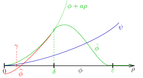
Figure 2.1. Construction of the function $\vartheta$.

Shrink $U$ so that $\rho:={\rm dist}_{L}^{2}:U\to{\mathbb{R}}$ is smooth and $J$-convex and $U=\{\rho<\varepsilon\}$. Since $\phi$ and $\psi$ agree to first order along $L$, we find an $a>0$ such that $\phi+a\rho>\psi$ on $U\setminus L$. An explicit computation shows that we can find a $J$-convex function $\bar{\phi}=\phi+f(\rho)$ which agrees with $\phi$ outside $U$ and with $\phi+a\rho$ on $\{\rho<\delta\}$ for some $\delta<\varepsilon$. Perturb $\bar{\phi}$ inside $\{\rho<\delta\}$ to a $J$-convex function $\widehat{\phi}$ with $\widehat{\phi}<\psi$ near $L$. Then the desired function $\vartheta$ is given by $\mathrm{smooth}\,\mathrm{max}(\psi,\widehat{\phi})$ on $\{\rho<\delta\}$, and $\widehat{\phi}$ outside. ∎

Corollary 2.8 (minimum construction for hypersurfaces).

Let $\Sigma,\Sigma^{\prime}$ be two compact $J$-convex hypersurfaces in a complex manifold $(V=M\times{\mathbb{R}},J)$ that are given as graphs of smooth functions $f,g:M\to{\mathbb{R}}$ and cooriented from below. Then there exists a $C^{0}$-close smooth approximation of ${\rm min}(f,g)$ whose graph $\Sigma^{\prime\prime}$ is $J$-convex.

Proof.

The functions $\phi(x,y):=y-f(x)$ and $\psi(x,y):=y-g(x)$ have $J$-convex zero sets $\Sigma=\phi^{-1}(0)$ and $\Sigma^{\prime}=\psi^{-1}(0)$. Note that the zero set of ${\rm max}(\phi,\psi)=y-{\rm min}(f,g)(x)$ is the graph of the function ${\rm min}(f,g)$. Now pick a convex increasing function $h:{\mathbb{R}}\to{\mathbb{R}}$ with $h(0)=0$ such that $h\circ\phi$ and $h\circ\psi$ are $J$-convex near $\Sigma$ resp. $\Sigma^{\prime}$, and define $\Sigma^{\prime\prime}$ as the zero set of $\mathrm{smooth}\,\mathrm{max}(h\circ\phi,h\circ\psi)$. ∎

Corollary 2.9 (from families of hypersurfaces to foliations).

Let $(M\times[0,1],J)$ be a compact complex manifold. Suppose there exists a smooth family of $J$-convex graphs (cooriented from below) $\Sigma_{\lambda}=\{y=f_{\lambda}(x)\}$, $\lambda\in[0,1]$, with $\Sigma_{0}=M\times\{0\}$ and $\Sigma_{1}=M\times\{1\}$. Then there exists a smooth foliation of $M\times[0,1]$ by $J$-convex graphs $\widetilde{\Sigma}_{\lambda}=\{y=\widetilde{f}_{\lambda}(x)\}$ $\lambda\in[0,1]$, with $\widetilde{\Sigma}_{0}=M\times\{0\}$ and $\widetilde{\Sigma}_{1}=M\times\{1\}$.

Proof.

By a family version of Corollary 2.8, the continuous functions $\bar{f}_{\lambda}:={\rm min}_{\mu\geq\lambda}f_{\mu}$ can be $C^{0}$-approximated by smooth functions $g_{\lambda}:M\to[0,1]$ whose graphs $\{y=g_{\lambda}(x)\}$ are $J$-convex. Since $\bar{f}_{\lambda}\leq\bar{f}_{\lambda^{\prime}}$ for $\lambda\leq\lambda^{\prime}$, this can be done in such a way that $g_{\lambda}\leq g_{\lambda^{\prime}}$ for $\lambda\leq\lambda^{\prime}$. So the graphs of $g_{\lambda}$ almost form a foliation, and stretching them slightly in the $y$-direction yields the desired foliation. ∎

Open question. Does an analogue of Proposition 2.5, or at least of Corollary 2.6, hold for non-integrable $J$? If this were true, then a lot of the theory in these notes would work in the non-integrable case.

$J$-convex model functions. Let us fix integers $1\leq k\leq n$. Consider ${\mathbb{C}}^{n}$ with complex coordinates $z_{j}=x_{j}+iy_{j}$, $j=1,\dots,n$, and set

$$R:=\sqrt{\sum_{j=1}^{k}x_{j}^{2}},\qquad r:=\sqrt{\sum_{j=k+1}^{n}x_{j}^{2}+\sum_{j=1}^{n}y_{j}^{2}}.$$

Fix some $a>1$ and define the standard $i$-convex function

$$\Psi_{\rm st}(r,R):=ar^{2}-R^{2}.$$

For small $\gamma>0$, we will use

$$H_{\gamma}:=\{r\leq\gamma,\;R\leq 1+\gamma\}$$

as a model for a complex $k$-handle. Its core disk is the totally real $k$-disk $\{r=0,\;R\leq 1+\gamma\}$ and it will be attached to the boundary of a Stein domain along the set $\{r\leq\gamma,\;R=1+\gamma\}$. The following theorem will allow us to extend a $J$-convex function over the handle.

Theorem 2.10.

For each $0<\gamma<1<a$ there exists an $i$-lc function $\Psi(r,R)$ on $H_{\gamma}$ with the following properties (see Figure 2.2):

1. $\Psi=\Psi_{\rm st}$ near $\partial H_{\gamma}$;

2. $\Psi$ has a unique index $k$ critical point at the origin;

3. the level set $\Sigma=\{\Psi=-1\}$ surrounds the core disk in the sense that $\{r=0,\;R\leq 1+\gamma\}\subset\{\Psi<-1\}$.

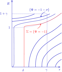
Figure 2.2. The function $\Psi_{1}$.

Proof.

Step 1. The first task is the construction of the hypersurface $\Sigma$. Let us write $\Sigma$ as a graph $R=\phi(r)$, which we allow to become vertical at $r=\delta$. One can work out the condition for $i$-convexity of $\Sigma$ (cooriented from above), which becomes a rather complicated system of second order differential inequalities for $\phi$. However, it turns out that if $\phi>0$, $\phi^{\prime}>0$, and $\phi^{\prime\prime}\leq 0$, the following simpler condition is sufficient for $i$-convexity:

(3) $$\phi^{\prime\prime}+\frac{\phi^{\prime 3}}{r}-\frac{1}{\phi}(1+\phi^{\prime 2})>0.$$

Step 2. To construct solutions of (3), we follow a suggestion by M. Struwe. We will find the function $\phi$ as a solution of Struwe’s equation

(4) $$\phi^{\prime\prime}+\frac{\phi^{\prime 3}}{2r}=0,$$

with $\phi^{\prime}>0$ and hence $\phi^{\prime\prime}<0$. Then (3) reduces to

(5) $$\frac{\phi^{\prime 3}}{2r}-\frac{1}{\phi}(1+\phi^{\prime 2})>0.$$

Now Struwe’s equation can be solved explicitly: It is equivalent to

$$\Bigl{(}\frac{1}{\phi^{\prime 2}}\Bigr{)}^{\prime}=-\frac{2\phi^{\prime\prime}}{\phi^{\prime 3}}=\frac{1}{r},$$

thus $1/\phi^{\prime 2}=\ln(r/\delta)$ for some constant $\delta>0$, or equivalently, $\phi^{\prime}(r)=1/\sqrt{\ln(r/\delta)}$. By integration, this yields a solution $\phi(r)$ for $r\geq\delta$ which is strictly increasing and concave and satisfies $\phi^{\prime}(\delta)=+\infty$. Choosing the remaining integration constant appropriately, we find a solution $\phi:[\delta,K\delta]\to{\mathbb{R}}$ which satisfies (5) and looks as shown in Figure 2.3. Here $d>0$ can be arbitrarily chosen and $K\delta$ can be made arbitrarily small.

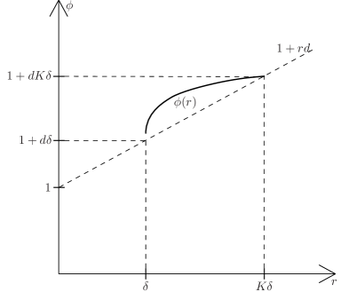
Figure 2.3. A solution of Struwe’s differential equation.

Step 3. Smoothing the maximum of the function $\phi$ from Step 2 and the linear function $L(r)=1+dr$ yields an $i$-convex hypersurface which surrounds the core disk and agrees with $\{R=L(r)\}$ for $r\geq K\delta$. To finish the construction of the hypersurface $\Sigma$ in Theorem 2.10, we still need to interpolate between $L(r)$ and the function $S(r)=\sqrt{1+ar^{2}}$ whose graph is the level set $\{\Psi_{\rm st}(r,R)=ar^{2}-R^{2}=-1\}$. Unfortunately, this cannot done directly with the maximum construction because the graph of $L$ ceases to define an $i$-convex hypersurface before it intersects the graph of $S$. The solution is to interpolate from $L$ to a quadratic function $Q(r)=1+br+cr^{2}/2$ and from there to $S$. The details are rather involved due to the fact that the simple sufficient condition (3) fails and one needs to invoke the full necessary and sufficient condition to ensure $i$-convexity during this interpolation.

Step 4. In Step 3 we constructed the level set $\Sigma$ as a graph $\{R=\phi(r)\}$. To construct the $i$-lc function $\Psi:H_{\gamma}\to{\mathbb{R}}$, in view of Corollary 2.9 it suffices to connect $\Sigma$ on both sides to level sets of $\Psi_{\rm st}$ by a smooth family of $i$-convex graphs. Towards larger $R$ this is a simple application of the maximum construction, whereas towards smaller $R$ it requires 1-parametric versions of the constructions in Steps 1-3. This proves Theorem 2.10. ∎

3. Existence of Stein structures

In this section we prove the Existence Theorem 1.5.

Step 1: Extension of complex structures over handles.
Consider an almost complex cobordism $(W,J)$ of complex dimension $n\geq 1$ such that $J$ is integrable near $\partial_{-}W$, and $\partial_{-}W$ is $J$-convex when cooriented by an inward pointing vector field. For $k\leq n$ consider an embedding $f:(D^{k},\partial D^{k})\hookrightarrow(W,\partial_{-}W)$, where $D^{k}\subset{\mathbb{R}}^{k}\subset{\mathbb{C}}^{n}$ is the closed unit disk.

Proposition 3.1.

The almost complex structure $J$ is homotopic rel ${\mathcal{O}}{\it p}\,(\partial_{-}W)$ to one which is integrable near $f(D^{k})$.

Proof.

After trivializing the relevant bundles, the differential of $f$ defines a map

$$df:(D^{k},\partial D^{k})\to(V_{2n,k},V_{2n-1,k-1}),$$

where $V_{m,\ell}$ is the Stiefel manifold of $\ell$-frames in ${\mathbb{R}}^{m}$. Let $V_{m,\ell}^{\mathbb{C}}\subset V_{2m,\ell}$ be the Stiefel manifold of complex $\ell$-frames in ${\mathbb{C}}^{m}$, or equivalently, of totally real $\ell$-frames in ${\mathbb{R}}^{2m}$.

Problem 3.2.

For each $n\geq 1$ and $k\leq n$, the map

$$\pi_{k}(V_{n,k}^{\mathbb{C}},V_{n-1,k-1}^{\mathbb{C}})\to\pi_{k}(V_{2n,k},V_{2n-1,k-1})$$

induced by the obvious inclusions is surjective.

Thus there exists a homotopy $F_{t}:(D^{k},\partial D^{k})\to(V_{2n,k},V_{2n-1,k-1})$ from $F_{0}=df$ to some $F_{1}:(D^{k},\partial D^{k})\to(V_{n,k}^{\mathbb{C}},V_{n-1,k-1}^{\mathbb{C}})$. Now a relative version of Gromov’s $h$-principle for totally real embeddings [15, 11] yields an isotopy of embeddings $f_{t}:(D^{k},\partial D^{k})\hookrightarrow(W,\partial_{-}W)$ from $f_{0}=f$ to a totally real embedding $f_{1}$.

By a further isotopy we can achieve that $f_{1}|_{\partial D^{k}}$ is real analytic. We complexify $f_{1}|_{\partial D^{k}}$ to a holomorphic embedding from a neighbourhood of $\partial D^{k}$ in ${\mathbb{C}}^{n}$ into a slight extension $\widetilde{W}$ of $W$ past $\partial_{-}W$, and then extend it to an embedding $\widetilde{f}_{1}:D^{k}\times D^{2n-k}_{\varepsilon}\hookrightarrow\widetilde{W}$ which agrees with $f_{1}$ on $D^{k}=D^{k}\times 0$ and whose differential is complex linear along $D^{k}$. The push-forward $(\widetilde{f}_{1})_{*}i$ of the standard complex structure $i$ on $D^{k}\times D^{2n-k}_{\varepsilon}\subset{\mathbb{C}}^{n}$ agrees with $J$ on a neighbourhood of $f_{1}(\partial D^{k})$ (since $\widetilde{f}_{1}$ is holomorphic there) and at points of $f_{1}(D^{k})$. Thus we can extend $(\widetilde{f}_{1})_{*}i$ to an almost complex structure $\widetilde{J}$ on $W$ which coincides with $J$ near $\partial_{-}W$ and outside a neighbourhood of $f_{1}(D^{k})$ and is integrable near $f_{1}(D^{k})$. An application of the isotopy extension theorem now yields the desired almost complex structure which coincides with $J$ near $\partial_{-}W$ and is integrable near the original disk $f(D^{k})$. ∎

By induction over the handles, Proposition 3.1 yields the following special case of the Gromov–Landweber theorem:

Corollary 3.3 (Gromov [14], Landweber [18]).

Let $(V,J)$ be an almost complex manifold of complex dimension $n\geq 1$ which admits an exhausting Morse function $\phi:V\to{\mathbb{R}}$ without critical points of index $>n$. Then $J$ is homotopic to an integrable complex structure. ∎

Step 2: Extension of $J$-convex functions over handles.
Consider again $(W,J)$ and $f:(D^{k},\partial D^{k})\hookrightarrow(W,\partial_{-}W)$ as in Step 1. After applying Proposition 3.1 we may assume that $J$ is integrable near $\Delta:=f(D^{k})$. After real analytic approximation and complexification, we may assume that $f$ extends to a holomorphic embedding $F:H_{\gamma}\hookrightarrow\widetilde{W}$, where $H_{\gamma}$ is the standard handle $D^{k}_{1+\gamma}\times D^{2n-k}_{\gamma}\subset{\mathbb{C}}^{n}$ and $\widetilde{W}$ is a slight extension of $W$ past $\partial_{-}W$.

Let $\phi$ be a given $J$-convex function near $\partial_{-}W=\{\phi=-1\}$. To finish the proof of Theorem 1.5, we need to extend $\phi$ to a $J$-convex function $\widetilde{\phi}$ on a neighbourhood of $\Delta$ whose level set $\{\widetilde{\phi}=-1\}$ coincides with $\partial_{-}W$ outside a neighbourhood of $\partial\Delta$ and surrounds $f(D^{k})$ in $W$ as shown in Figure 3.1.

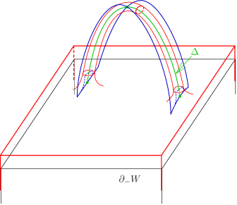
Figure 3.1. Surrounding a $J$-orthogonally attached totally real disk.

Equivalently, we need to extend $F^{*}\phi$ to an $i$-convex function $\Psi$ on $H_{\gamma}$ whose level set $\{\Psi=-1\}$ coincides with $\{F^{*}\phi=-1\}$ near $\partial H_{\gamma}$ and surrounds $D^{k}$ in $H_{\gamma}$. According to Theorem 2.10 in the previous section, this can be done if we can arrange that $F^{*}\phi$ equals the standard function $\Psi_{\rm st}(r,R)=ar^{2}-R^{2}$ near $\partial D^{k}$.

To analyze the last condition, note that the $n$-disk $D^{n}$ meets the level set $\{\Psi_{\rm st}=-1\}$ $i$-orthogonally along $\partial D^{n}$ in the sense that $i(T_{x}D^{n})\subset T_{x}\Sigma$ for all $x\in\partial D^{n}$. Conversely, suppose that $D^{n}$ is $i$-orthogonal to the level set $\{F^{*}\phi=-1\}$ along $\partial D^{k}$. Then $F^{*}\phi$ and $\Psi_{\rm st}$ have the same kernel $T_{x}\partial D^{n}\oplus i(T_{x}D^{n})$ at $x\in\partial D^{k}$. After rescaling we may assume that $F^{*}\phi$ agrees with $\Psi_{\rm st}$ to first order along $\partial D^{k}$, so by Corollary 2.7 we can deform $F^{*}\phi$ to make it coincide with $\Psi_{\rm st}$ near $\partial D^{k}$.

The preceding discussion shows that it suffices to arrange that $F(D^{n}\cap H_{\gamma})$ is $J$-orthogonal to $\partial_{-}W$ along $\partial\Delta=f(\partial D^{k})$. This can be arranged by appropriate choice of the extension $F$ provided that $\Delta$ is $J$-orthogonal to $\partial_{-}W$ along $\partial\Delta$. Note that a necessary condition for this is $JT_{x}\partial\Delta\subset T_{x}\partial_{-}W$ for $x\in\partial\Delta$, which means that $\partial\Delta$ is isotropic for the contact structure $\xi=T\partial_{-}W\cap J(T\partial_{-}W)$ on $\partial_{-}W$. Conversely, if this condition holds it is not hard to arrange $J$-orthogonality. So we have reduced the proof of Theorem 1.5 to

Proposition 3.4.

Consider an almost complex cobordism $(W,J)$ of complex dimension $n$ such that $J$ is integrable near $\partial_{-}W$, and $\partial_{-}W$ is $J$-convex when cooriented by an inward pointing vector field. If $n>2$, then any embedding $f:(D^{k},\partial D^{k})\hookrightarrow(W,\partial_{-}W)$, $k\leq n$, is isotopic to one which is totally real on $D^{k}$ and isotropic on $\partial D^{k}$.

The remainder of this section is devoted to the proof of this proposition.

The subcritical case. Recall from Step 1 that there exists a homotopy $F_{t}:(D^{k},\partial D^{k})\to(V_{2n,k},V_{2n-1,k-1})$ from $F_{0}=df$ to some $F_{1}:(D^{k},\partial D^{k})\to(V_{n,k}^{\mathbb{C}},V_{n-1,k-1}^{\mathbb{C}})$. Restricting it to the boundary provides a homotopy $G_{t}=F_{t}|_{\partial D^{k}}:\partial D^{k}\to V_{2n-1,k-1}$ from $G_{0}=df|_{\partial D^{k}}$ to some $G_{1}:\partial D^{k}\to V_{n-1,k-1}^{\mathbb{C}}$. Now Gromov’s $h$-principle for isotropic immersions [15, 11] yields a homotopy of immersions $g_{t}:\partial D^{k}\to\partial_{-}W$ from $g_{0}=f|_{\partial D^{k}}$ to an isotropic immersion $g_{1}$ together with a 2-parameter family of maps $G_{t}^{s}:\partial D^{k}\to V_{2n-1,k-1}$ satisfying $G_{t}^{0}=dg_{t}$, $G_{t}^{1}=G_{t}$, $G_{0}^{s}=dg_{0}$, and $G_{1}^{s}:\partial D^{k}\to V_{n-1,k-1}^{\mathbb{C}}$ for all $s,t\in[0,1]$.

If the $g_{t}$ can be chosen to be embeddings rather than immersions, then the $h$-principle for totally real embeddings allows us to extend the $g_{t}$ to embeddings $f_{t}:D^{k}\hookrightarrow W$ with $f_{1}$ totally real and the proposition follows. In the subcritical case $k<n$, this can be achieved simply by a generic perturbation of the $g_{t}$ (keeping $g_{1}$ isotropic).

Remark 3.5.

The existence of the 2-parameter family $G_{t}^{s}$ is crucial for the application of the $h$-principle for totally real embeddings. Indeed, we can always connect $g_{0}=f|_{\partial D^{k}}$ by embeddings $g_{t}$ to some isotropic embedding $g_{1}$, so if we could extend these $g_{t}$ to totally real embeddings $D^{k}\hookrightarrow W$ we would prove Proposition 3.4 also in the case $k=n=2$ where, as we shall see below, it is false in general.

The critical case. In the critical case $k=n$, we can still perturb $g_{1}$ to a Legendrian embedding, but the $g_{t}$ need not all be embeddings. To understand the obstruction to this, consider the immersion

$$\Gamma:S^{n-1}\times[0,1]\to\partial_{-}W\times[0,1],\qquad(x,t)\mapsto\bigl{(}g_{t}(x),t\bigr{)}.$$

After a generic perturbation, we may assume that $\Gamma$ has finitely many transverse self-intersections and define its self-intersection index

$$I_{\Gamma}:=\sum_{p}I_{\Gamma}(p)\in\begin{cases}{\mathbb{Z}}&\text{ if $n$ is even,}\\ {\mathbb{Z}}_{2}&\text{ if $n$ is odd}\end{cases}$$

as the sum over the indices of all self-intersection points $p$. Here the index $I_{\Gamma}(p)=\pm 1$ is defined by comparing the orientations of the two intersecting branches of $\Gamma$ to the orientation of $\partial_{-}W\times[0,1]$. For $n$ even this does not depend on the order of the branches and thus gives a well-defined integer, while for $n$ odd it is only well-defined mod $2$. By a theorem of Whitney [27], for $n>2$, the regular homotopy $g_{t}$ can be deformed through regular homotopies fixed at $t=0,1$ to an isotopy iff $I_{\Gamma}=0$.

So if the family $g_{t}$ satisfies $I_{\Gamma}=0$ we are done. If $I_{\Gamma}\neq 0$ we will connect $g_{1}$ to another Legendrian embedding $g_{2}$ by a Legendrian regular homotopy $g_{t}$, $t\in[1,2]$, whose self-intersection index equals $-I_{\Gamma}$. The extended family $g_{t}$, $t\in[0,2]$, then has self-intersection index zero, so applying the previous argument to this family will conclude the proof.

Stabilization of Legendrian submanifolds. Consider a Legendrian submanifold $\Lambda_{0}$ in a contact manifold $(M,\xi)$ of dimension $2n-1$. Near a point of $\Lambda_{0}$ pick Darboux coordinates $(q_{1},p_{1},\dots,q_{n-1},p_{n-1},z)$ in which $\xi=\ker(dz-\sum_{j}p_{j}dq_{j})$ and the front projection of $\Lambda_{0}$ is a standard cusp $z^{2}=q_{1}^{3}$. Deform the two branches of the front to make them parallel over some open ball $B^{n-1}\subset{\mathbb{R}}^{n-1}$. After rescaling, we may thus assume that the front of $\Lambda_{0}$ has two parallel branches $\{z=0\}$ and $\{z=1\}$ over $B^{n-1}$, see Figure 3.2.

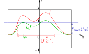
Figure 3.2. Stabilization of a Legendrian submanifold.

Pick a non-negative function $f:B^{n-1}\to{\mathbb{R}}$ with compact support and $1$ as a regular value, so $N:=\{f\geq 1\}\subset B^{n-1}$ is a compact manifold with boundary. Replacing for each $t\in[0,1]$ the lower branch $\{z=0\}$ by the graph $\{z=tf(q)\}$ of the function $tf$ yields the fronts of a path of Legendrian immersions $\Lambda_{t}\subset M$ connecting $\Lambda_{0}$ to a new Legendrian submanifold $\Lambda_{1}$. Note that $\Lambda_{t}$ has a self-intersection for each critical point of $tf$ on level $1$.

Problem 3.6.

The Legendrian regular homotopy $\Lambda_{t}$, $t\in[0,1]$, has self-intersection index $(-1)^{(n-1)(n-2)/2}\chi(N)$.

Problem 3.7.

For $n>2$ there exist compact submanifolds $N\subset{\mathbb{R}}^{n-1}$ of arbitrary Euler characteristic $\chi(N)\in{\mathbb{Z}}$, while for $n=2$ the Euler characteristic is always positive.

These two problems show that for $n>2$ the stabilization construction allows us find a Legendrian regular homotopy $\Lambda_{t}$, $t\in[0,1]$, with arbitrary self-intersection index. In view of the discussion above, this concludes the proof of Proposition 3.4 and hence of Theorem 1.5. $\Box$

Remark 3.8.

The condition $n>2$ was used twice in the proof of Proposition 3.4: for the application of Whitney’s theorem, and to arbitrarily modify the self-intersection index by stabilization.

To illustrate the failure of Theorem 1.5 for $n=2$, let us analyze for which oriented plane bundles $V\to S^{2}$ the total space admits a Stein structure. Here $V$ is oriented by minus the orientation of the base followed by that of the fibre. Such bundles are classified by their Euler class $e(V)$, which equals minus the self-intersection number $S\cdot S\in{\mathbb{Z}}$ of the zero section $S\subset V$.

We can construct each such bundle by attaching a 2-handle to the 4-ball $B^{4}$ along a topologically trivial Legendrian knot $\Lambda\subset(S^{3},\xi_{\rm st})$. Let $\Delta\subset B^{4}$ be an embedded 2-disk meeting $\partial B^{4}$ transversely along $\partial\Delta=\Lambda$. It fits together with the core disk $D$ of the handle to an embedded 2-sphere $S\subset V$ giving the zero section in $V$. Recall that the Thurston-Bennequin invariant ${\rm tb}(\Lambda)$ is defined as the linking number of $\Lambda$ with a push-off $\Lambda^{\prime}$ in the direction of a Reeb vector field on $(S^{3},\xi_{\rm st})$.

Problem 3.9.

The complex structure on $B^{4}\subset{\mathbb{C}}^{2}$ extends to a complex structure on $V$ for which the core disk $D$ is totally real (and hence by Theorem 1.5 to a Stein structure on $V$) iff $-e(V)=S\cdot S={\rm tb}(\Lambda)-1$.

In view of Bennequin’s inequality ${\rm tb}(\Lambda)\leq-1$, this shows that the construction of Theorem 1.5 works to provide a Stein structure on $V$ iff $e(V)\geq 2$. A much deeper theorem of Lisca and Matič [19] (proved via Seiberg-Witten theory) asserts that $S\cdot S\leq-2$ for every homologically nontrivial embedded 2-sphere $S$ in a Stein surface, hence $V$ admits a Stein structure iff $e(V)\geq 2$. For example, the manifold $S^{2}\times{\mathbb{R}}^{2}$ does not admit any Stein structure.

4. Morse-Smale theory for $J$-convex functions

Morse-Smale theory deals with the problem of simplification of a Morse function, trying to remove as many critical points as the topology allows. One consequence is the $h$-cobordism theorem and the proof of the higher-dimensional Poincaré conjecture. In this section we study Morse-Smale theory for $J$-convex Morse functions, resulting in a Stein version of the $h$-cobordism theorem.

The $h$-cobordism theorem. Let us begin by recalling the celebrated

Theorem 4.1 ($h$-cobordism theorem, Smale [26]).

Let $W$ be an $h$-cobordism, i.e., a compact cobordism such that $W$ and $\partial_{\pm}W$ are simply connected and $H_{*}(W,\partial_{-}W;{\mathbb{Z}})=0$. Suppose that $\dim W\geq 6$. Then $W$ carries a function without critical points and constant on $\partial_{\pm}W$.

For the proof, one considers a compact cobordism $W$ with a Morse function $\phi:W\to{\mathbb{R}}$ having $\partial_{\pm}W$ as regular level sets and a gradient-like vector field $X$ for $\phi$. We will refer to such $(W,X,\phi)$ as a Smale cobordism. It is called elementary if $W_{p}^{-}\cap W_{q}^{+}=\emptyset$ for all critical points $p\neq q$, where $W_{p}^{-}$ and $W_{p}^{+}$ denotes the stable resp. unstable manifold of $p$ with respect to $X$.

The key geometric ingredients in the proof of the $h$-cobordism theorem are the following four geometric lemmas about modifications of Smale cobordisms (see [21]). The first three of them are rather simple, while the fourth one is more difficult.

Lemma 4.2 (moving critical levels).

Let $(W,X,\phi_{0})$ be an elementary Smale cobordism. Then there exists a homotopy $(W,X,\phi_{t})$ of elementary Smale cobordisms which arbitrarily changes the ordering of the values of the critical points.

Lemma 4.3 (moving attaching spheres).

Let $(W,X_{0},\phi)$ be a Smale cobordism and $p\in W$ a critical point whose stable manifold $W_{p}^{-}(X_{0})$ with respect to $X_{0}$ intersects $\partial_{-}W$ along a sphere $S_{0}\subset\partial_{-}W$. Then given any isotopy $S_{t}\subset\partial_{-}W$, $t\in[0,1]$, there exists a homotopy of Smale cobordisms $(W,X_{t},\phi)$ such that the stable manifold $W^{-}_{p}(X_{t})$ intersects $\partial_{-}W$ along $S_{t}$.

Lemma 4.4 (creation of critical points).

Let $(W,X_{0},\phi_{0})$ be a Smale cobordism without critical points. Then for any $1\leq k\leq\dim W$ and any $p\in{\rm Int\,}W$ there exists a Smale homotopy $(W,X_{t},\phi_{t})$, $t\in[0,1]$, fixed outside a neighbourhood of $p$, which creates a pair of critical points of index $k-1$ and $k$ connected by a unique trajectory of $X_{1}$ along which the stable and unstable manifolds intersect transversely.

Lemma 4.5 (cancellation of critical points).

Suppose that a Smale cobordism $(W,X_{0},\phi_{0})$ contains exactly two critical points of index $k-1$ and $k$ which are connected by a unique trajectory of $X$ along which the stable and unstable manifolds intersect transversely. Then there exists a Smale homotopy $(W,X_{t},\phi_{t})$, $t\in[0,1]$, which kills the critical points, so the cobordism $(W,X_{1},\phi_{1})$ has no critical points.

Here all the homotopies will be fixed on a neighbourhood of $\partial_{\pm}W$. The functions $\phi_{t}$ in Lemmas 4.4 and 4.5 will be Morse except for one value $t_{0}\in(0,1)$ where they have a birth-death type critical point. Here a birth-death type critical point of index $k-1$ at $t_{0}$ is described by the local model

$$\phi_{t}(x)=x_{1}^{3}\mp(t-t_{0})x_{1}-x_{2}^{2}-\dots-x_{k}^{2}+x_{k+1}^{2}+\dots+x_{m}^{2}.$$

Problem 4.6.

Prove Lemmas 4.2, 4.3 and 4.4.

Modifications of $J$-convex Morse functions. Let us now state the analogues of the four lemmas for $J$-convex functions. By a Stein cobordism $(W,J,\phi)$ we will mean a complex cobordism $(W,J)$ with a $J$-convex Morse function $\phi:W\to{\mathbb{R}}$ having $\partial_{\pm}W$ as regular level sets. We will always use the gradient vector field $\nabla_{\phi}\phi$ of $\phi$ with respect to the metric $g_{\phi}=-dd^{\mathbb{C}}\phi(\cdot,J\cdot)$ to obtain a Smale cobordism $(W,\nabla_{\phi}\phi,\phi)$. Note that in the following four propositions the complex structure $J$ is always fixed.

Proposition 4.7 (moving critical levels).

Let $(W,J,\phi_{0})$ be an elementary Stein cobordism. Then there exists a homotopy $(W,J,\phi_{t})$ of elementary Stein cobordisms which arbitrarily changes the ordering of the values of the critical points.

Proposition 4.8 (moving attaching spheres).

Let $(W,J,\phi_{0})$ be a Stein cobordism and $p\in W$ a critical point whose stable manifold $W_{p}^{-}(\phi_{0})$ with respect to $\nabla_{\phi_{0}}\phi_{0}$ intersects $\partial_{-}W$ along an isotropic sphere $S_{0}\subset\partial_{-}W$. Then given any isotropic isotopy $S_{t}\subset\partial_{-}W$, $t\in[0,1]$, there exists a homotopy of Stein cobordisms $(W,J,\phi_{t})$ with fixed critical point $p$ such that the stable manifold $W^{-}_{p}(\phi_{t})$ intersects $\partial_{-}W$ along $S_{t}$.

Proposition 4.9 (creation of critical points).

Let $(W,J,\phi_{0})$ be a Stein cobordism without critical points. Then for any $1\leq k\leq\dim_{\mathbb{C}}W$ and any $p\in{\rm Int\,}W$ there exists a Stein homotopy $(W,J,\phi_{t})$, $t\in[0,1]$, fixed outside a neighbourhood of $p$, which creates a pair of critical points of index $k-1$ and $k$ connected by a unique trajectory of $\nabla_{\phi_{1}}\phi_{1}$ along which the stable and unstable manifolds intersect transversely.

Proposition 4.10 (cancellation of critical points).

Suppose that a Stein cobordism $(W,J,\phi_{0})$ contains exactly two critical points of index $k-1$ and $k$ which are connected by a unique trajectory of $\nabla_{\phi_{0}}\phi_{0}$ along which the stable and unstable manifolds intersect transversely. Then there exists a Stein homotopy $(W,J,\phi_{t})$, $t\in[0,1]$, which kills the critical points, so the cobordism $(W,J,\phi_{1})$ has no critical points.

Again, all the homotopies will be fixed on a neighbourhood of $\partial_{\pm}W$, up to composition of the $J$-convex functions with some convex increasing function ${\mathbb{R}}\to{\mathbb{R}}$. The statements are precise analogues of those in the smooth case, with one notable difference: in Proposition 4.8 we require the isotopy $S_{t}$ to be isotropic. This difference, and the lack of a 1-parametric $h$-principle for Legendrian embeddings, is largely responsible for all symplectic rigidity phenomena on Stein manifolds. However, in the subcritical case ${\rm ind}(p)=k<n$ we have an $h$-principle stating that any smooth isotopy $S_{t}$ starting at an isotropic embedding $S_{0}$ can be $C^{0}$-approximated by an isotropic isotopy starting at $S_{0}$. With this, the proof of the $h$-cobordism theorem goes through for $J$-convex functions and we obtain

Theorem 4.11 (Stein $h$-cobordism theorem).

Let $(W,J,\phi)$ be a subcritical Stein $h$-cobordism. Suppose that $\dim_{\mathbb{C}}W\geq 3$. Then $W$ carries a $J$-convex function without critical points and constant on $\partial_{\pm}W$.

Further implications of these results will be discussed in Section 5. The remainder of this section is devoted to the proofs of Propositions 4.7 to 4.10.

Proof of Proposition 4.7.

This is an immediate consequence of the $J$-convex model functions constructed in Section 3: Since the cobordism is elementary, the stable manifolds of the critical points are disjoint embedded disks. For each critical point $p$, Theorem 2.10 allows us to deform $\phi_{0}$ near $W_{p}^{-}$ such that for the new $J$-lc function the level set containing $p$ is connected to a level set of $\phi_{0}$ slightly above $\partial_{-}W$. Now we perform this operation for each critical point and choose the level sets near $\partial_{-}W$ to achieve any given ordering. ∎

Proof of Proposition 4.8.

Let $k:={\rm ind}(p)\leq n$. We identify level sets of $\phi_{0}$ near $\partial_{-}W$ via Gray’s theorem. Then we construct an isotopy of embedded $k$-disks $D_{t}\subset W$ such that $D_{0}=W_{p}^{-}$, $D_{t}$ agrees with $W_{p}^{-}$ near $p$, $\partial D_{t}=S_{t}$, and $D_{t}$ intersects all level sets of $\phi$ below $c:=\phi(p)$ transversely in isotropic $(k-1)$-spheres; see Figure 4.1.

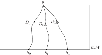
Figure 4.1. Moving attaching spheres by isotropic isotopies.

The last condition implies that $D_{t}$ is totally real. If $k<n$ we can further extend $D_{t}$ to a totally real embedding of $D^{k}\times D^{n-k}_{\varepsilon}$ intersecting level sets transversely in isotropic submanifolds, so it suffices to consider the case $k=n$. To conclude the proof, we will construct $J$-convex functions $\phi_{t}$ which agree with $\phi_{0}$ near $p$ and whose gradient $\nabla_{\phi_{t}}\phi_{t}$ is tangent to $D_{t}$. This is done in two steps.

In the first step we construct $J$-convex functions $\psi_{t}$ whose level sets below $c$ are $J$-orthogonal to $D_{t}$. To do this, consider some level set $\Sigma$ of $\phi_{0}$ intersecting $D_{t}$ in the isotropic submanifold $\Lambda_{t}$. Let $\xi$ be the induced contact structure on $\Sigma$. We deform $\Sigma$ near $\Lambda_{t}$ to a new hypersurface $\Sigma^{\prime}$ which agrees with $\Sigma$ outside a neighbourhood of $\Lambda_{t}$, intersects $D_{t}$ $J$-orthogonally in $\Lambda_{t}$, and satisfies $\xi\subset T\Sigma^{\prime}$ along $\Lambda_{t}$ (so we “turn $\Sigma$ around $\xi$ along $\Lambda_{t}$”); see Figure 4.2.

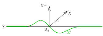
Figure 4.2. Turning a $J$-convex hypersurface along an isotropic submanifold.

A careful estimate of the Levi form shows that $\Sigma^{\prime}$ can be made $J$-convex. Deforming all level sets in this way leads to a family of $J$-convex hypersurfaces, which by Corollary 2.9 can be turned into a foliation and thus into level sets of a $J$-lc function.

For the second step, consider the $J$-convex functions $\psi_{t}$ from the first step whose level sets below $c$ are $J$-orthogonal to $D_{t}$. It is not hard to write down in a local model a $J$-convex function $\vartheta_{t}$ near $D_{t}$ which agrees with $\psi_{t}$ on $D_{t}$, whose level sets are $J$-orthogonal to $D_{t}$, and whose gradient $\nabla_{\vartheta_{t}}\vartheta_{t}$ is tangent to $D_{t}$. Now Corollary 2.7 provides the desired function $\phi_{t}$ which coincides with $\psi_{t}$ outside a neighbourhood of $D_{t}$ and with $\vartheta_{t}$ in a smaller neighborhood of $D_{t}$. ∎

Proof of Proposition 4.10.

Let $(W,J,\phi_{0})$ be a Stein cobordism with exactly two critical points $p$, $q$ of index $k$, $k-1$ connected by a unique trajectory of $\nabla_{\phi_{0}}\phi_{0}$ along which the stable and unstable manifolds intersect transversely. Set $a:=\phi_{0}|_{\partial_{-}W}$, $b:=\phi_{0}(q)$ and $c:=\phi_{0}(p)$.

Problem 4.12.

In the situation above, suppose that $\phi_{0}$ is quadratic in some holomorphic coordinates near $p$ and $q$. Then the closure of $W_{p}^{-}$ is an embedded $k$-dimensional half-disk $\Delta\subset W$ with lower boundary $\partial_{-}\Delta=\Delta\cap\partial_{-}W$ and upper boundary $\partial_{+}\Delta=W_{q}^{-}$; see Figure 4.3.

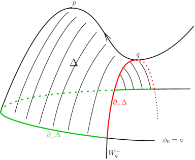
Figure 4.3. The half-disk $\Delta$.

We will now deform the function $\phi_{0}$ in 4 steps. The first 3 steps modify $\phi_{0}$ outside $\Delta$, without affecting its critical points, to make some level set closely surround $\Delta$; the actual cancellation happens in the last step.

First surrounding. First we apply Theorem 2.10 to the $(k-1)$-disk $\partial_{+}\Delta$ to deform $\phi_{0}$ to a $J$-lc function $\phi_{1}$ such that some level set $\Sigma_{1}=\{\phi_{1}=c_{1}\}$ closely surrounds $\partial_{+}\Delta$ as shown in Figure 4.4.

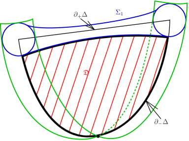
Figure 4.4. The first surrounding hypersurface $\Sigma_{1}$ and the disk $\mathfrak{D}$.

Second surrounding. Next we apply Theorem 2.10 to the $k$-disk $\mathfrak{D}:=\Delta\cap\{\phi_{1}\geq c_{1}\}$ to deform $\phi_{1}$ to a $J$-lc function $\phi_{2}$ such that some level set $\Sigma_{2}=\{\phi_{2}=c_{2}\}$ closely surrounds $\Delta$ as shown in Figure 4.4. Note that a cross-section of $\Sigma_{2}$ will have a dumbell-like shape as in Figure 4.5, where $x=(x_{1},\dots,x_{k})$ and $u=(x_{k+1},\dots,x_{n},y_{1},\dots,y_{n})$.

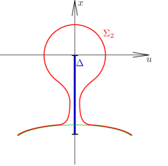
Figure 4.5. The dumbell-shaped cross-section of the second surrounding hypersurface $\Sigma_{2}$.

Third surrounding. On the other hand, we can construct another hypersurface $\Sigma_{3}$ surrounding $\Delta$ as follows: Restrict a very thin model hypersurface $\Sigma$ provided by Theorem 2.10 to a neighbourhood of the lower half-disk $\{r=0,R\leq 1,y_{k}\leq 0\}$ in ${\mathbb{C}}^{n}$, implant it onto a neighbourhood of $\Delta$ in $W$, and apply the minimum construction in Corollary 2.8 to this hypersurface and $\Sigma_{2}$. The resulting $J$-convex hypersurface $\Sigma_{3}$ is shown in Figure 4.6.

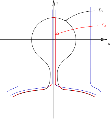
Figure 4.6. The third surrounding hypersurface $\Sigma_{3}$.

The most difficult part is now to connect $\Sigma_{3}$ to $\Sigma_{2}$ by a family of $J$-convex hypersurfaces. Once this is done, we can apply Corollary 2.9 to deform $\phi_{2}$ to a $J$-lc function $\phi_{3}$ having $\Sigma_{3}$ as a level set.

The cancellation. Let us extend $\Delta$ across $\partial_{+}\Delta$ to a slightly larger half-disk $\Delta^{\prime}$, still surrounded by $\Sigma_{3}$, so that the critical points $p,q$ lie in the interior of $\Delta^{\prime}$, and $\nabla_{\phi_{3}}\phi_{3}$ is inward pointing along $\partial_{-}\Delta^{\prime}$ and outward pointing along $\partial_{+}\Delta^{\prime}$. By Lemma 4.5 there exists a family of smooth functions $\beta_{t}:\Delta^{\prime}\to{\mathbb{R}}$, $t\in[3,4]$, fixed near $\partial\Delta^{\prime}$, such that $\beta_{3}=\phi_{3}|_{\Delta^{\prime}}$ and $\beta_{4}$ has no critical points. Identifying $\Delta^{\prime}$ with the lower half-disk in the standard handle, we can pick a large constant $B>0$ such that the functions $\psi_{t}:=\beta_{t}+Br^{2}$ near $\Delta^{\prime}$ are $J$-convex for all $t\in[3,4]$.

After an application of Corollary 2.7, we may assume that $\psi_{3}=\phi_{3}$ near $\Delta^{\prime}$. We can choose convex increasing functions $f_{t}:{\mathbb{R}}\to{\mathbb{R}}$ with $f_{3}={\rm id}$ such that for $t\in[3,4]$ the $J$-convex function $\phi_{t}:=\mathrm{smooth}\,\mathrm{max}(\psi_{t},f_{t}\circ\phi_{3})$ agrees with $f_{t}\circ\phi_{3}$ in the region outside of $\Sigma_{3}$ and with $\psi_{t}$ near $\Delta^{\prime}$. In particular, $\phi_{4}$ has no critical points (for this one needs to check that the maximum constructon does not create new critical points outside $\Delta^{\prime}$). Hence $(W,J,\phi_{4t})$, $t\in[0,1]$, is the desired Stein homotopy and Proposition 4.10 is proved. ∎

Proof of Proposition 4.9.

The proof is similar to that of Proposition 4.10 but much simpler. Set $a:=\phi_{0}|_{\partial_{-}W}$ and $c:=\phi_{0}(p)$. Pick an isotropic embedded $(k-1)$-sphere $S$ through $p$ in the level set $\phi_{0}^{-1}(c)$ and let $Z\subset W$ be the totally real cylinder swept out by $S$ under the backward gradient flow of $\phi_{0}$. We identify $Z$ with the cylinder $\{r=0,1/2\leq R\leq 1\}$ in the standard handle. A slight modification of Theorem 2.10 yields a family of $J$-convex functions $\phi_{t}:W\to{\mathbb{R}}$, $t\in[0,1]$, such that some level set $\Sigma_{1}$ of $\phi_{1}$ surrounds $Z$ in $W$.

By Lemma 4.4 there exists a family of smooth functions $\beta_{t}:Z\to{\mathbb{R}}$, $t\in[1,2]$, fixed near $\partial Z$, such that $\beta_{1}=\phi_{1}|_{Z}$ and $\beta_{2}$ has exactly two critical points of index $k-1$ and $k$ connected by a unique gradient trajectory along which the stable and unstable manifolds intersect transversely. As above, we can pick a large constant $B>0$ such that the functions $\psi_{t}:=\beta_{t}+Br^{2}$ near $Z$ are $J$-convex for all $t\in[1,2]$ and set $\phi_{t}:=\mathrm{smooth}\,\mathrm{max}(\psi_{t},f_{t}\circ\phi_{1})$, $t\in[1,2]$, to obtain the desired family $\phi_{2t}$, $t\in[0,1]$. ∎

5. Flexibility of Stein structures

In this section we study the question when two Stein structures on the same manifold can be connected by a Stein homotopy.

Stein homotopies. Let us first carefully define the notion of a Stein homotopy. Consider first a smooth family (with respect to the $C^{\infty}_{\rm loc}$-topology) of exhausting functions $\phi_{t}:V\to{\mathbb{R}}$, $t\in[0,1]$, on a manifold $V$. We call it a simple Morse homotopy if there exists a family of smooth functions $c_{1}<c_{2}<\dots$ on the interval $[0,1]$ such that for each $t\in[0,1]$, $c_{i}(t)$ is a regular value of the function $\phi_{t}$ and $\bigcup_{k}\{\phi_{t}\leq c_{k}(t)\}=V$. Then a Morse homotopy is a composition of finitely many simple Morse homotopies, and a Stein homotopy is a family of Stein structures $(V,J_{t},\phi_{t})$ such that the functions $\phi_{t}$ form a Morse homotopy.

The role of the regular levels $c_{i}(t)$ is to prevent critical points from “escaping to infinity”. The following three problems motivate why this is the correct definition. The first one shows that, without this condition, the notion of “homotopy” would become rather trivial:

Problem 5.1.

Any two Stein structures $(J_{0},\phi_{0})$ and $(J_{1},\phi_{1})$ on ${\mathbb{C}}^{n}$ can be connected by a smooth family of Stein structures $(J_{t},\phi_{t})$ on ${\mathbb{C}}^{n}$, allowing critical points to escape to infinity.

The second one shows that the question whether two Stein structures are homotopic does not depend on the chosen $J$-convex functions:

Problem 5.2.

If $\phi_{0},\phi_{1}:V\to{\mathbb{R}}$ are two exhausting $J$-convex functions for the same complex structure $J$, then $(J,\phi_{0})$ and $(J,\phi_{1})$ can be connected by a Stein homotopy $(J,\phi_{t})$.

The third one makes the question of Stein homotopies accessible to symplectic techniques. Let us call a Stein structure $(J,\phi)$ complete if the gradient vector field $\nabla_{\phi}\phi$ is complete; by Problem 2.2, any Stein structure can be made complete by composing $\phi$ with a convex increasing function $f:{\mathbb{R}}\to{\mathbb{R}}$.

Problem 5.3.

If two complete Stein structures $(J_{0},\phi_{0})$ and $(J_{1},\phi_{1})$ on a manifold $V$ are Stein homotopic, then the associated symplectic manifolds $(V,-dd^{\mathbb{C}}\phi_{0})$ and $(V,-dd^{\mathbb{C}}\phi_{1})$ are symplectomorphic.

From now on, when we talk about individual Stein structures $(J,\phi)$ we will always assume that the function $\phi$ is Morse, while for Stein homotopies we allow birth-death type singularities.

The 2-index theorem. Before studying Stein homotopies, let us first consider the situation in smooth topology. It follows from Problem 5.2 (simply ignoring $J$-convexity) that any two Morse functions on the same manifold can be connected by a Morse homotopy. In addition, we will need some control over the indices of critical points. This is provided by following immediate consequence of the two-index theorem of Hatcher and Wagoner ([16], see also [17]):

Theorem 5.4.

Let $\phi_{0},\phi_{1}:W\to[0,1]$ be two Morse functions on an $m$-dimensional cobordism $W$ with $\partial_{\pm}W$ as regular level sets. For some $k\geq 3$, suppose that $\phi_{0},\phi_{1}$ have no critical points of index $>k$. Then $\phi_{0}$ and $\phi_{1}$ can be connected by a Morse homotopy $\phi_{t}$ (all having $\partial_{\pm}W$ as regular level sets) without critical points of index $>k$.

We will apply this theorem in the following two cases with $m=2n$:

• the subcritical case $k+1=n\geq 4$;

• the critical case $k=n\geq 3$.

Uniqueness of subcritical Stein structures. After these preparations, we can prove our first uniqueness theorem.

Theorem 5.5 (uniqueness of subcritical Stein structures).

Let $(J_{0},\phi_{0})$ and $(J_{1},\phi_{1})$ be two subcritical Stein structures on the same manifold $V$ of complex dimension $n>3$. If $J_{0}$ and $J_{1}$ are homotopic as almost complex structures, then $(J_{0},\phi_{0})$ and $(J_{1},\phi_{1})$ are Stein homotopic.

Proof.

By Theorem 5.4 with $k+1=n\geq 4$, the functions $\phi_{0}$ and $\phi_{1}$ can be connected a Morse homotopy $\phi_{t}$ without critical points of index $\geq n$. We cut the homotopy into a finite number of simple Morse homotopies, and we cut each simple homotopy at the regular levels $c_{i}$ into countably many compact cobordisms. Let us pick gradient-like vector fields $X_{t}$ for $\phi_{t}$. After further decomposition of these cobordisms, we may assume that on each cobordism $W$ only one of the following two cases occurs:

1. all the Smale cobordisms $(W,X_{t},\phi_{t})$ are elementary;

2. a pair of critical points is created or cancelled.

In the first case, only the levels of the critical points vary and the ataching spheres move by smooth isotopies. By the $h$-principle for subcritical isotropic embeddings, these isotopies can be $C^{0}$-approximated by isotropic isotopies. So we can apply Propositions 4.7 and 4.8 to realize the same moves by $J$-convex functions. The second case is treated by Propositions 4.9 and 4.10. Applying the four propositions inductively over the simple homotopies, and within each simple homotopy over increasing levels, we hence construct a family of $J_{0}$-convex functions (all for the same $J_{0}$!) $\psi_{t}:V\to{\mathbb{R}}$ such that $\psi_{t}=\phi_{t}\circ h_{t}$ for a smooth family of diffeomorphisms $h_{t}:V\to V$ with $h_{0}={\rm id}$.

Note that $\bigl{(}(h_{t})_{*}J_{0},\phi_{t}\bigr{)}$ provides a Stein homotopy from $(J_{0},\phi_{0})$ to $\bigl{(}J_{2}:=(h_{1})_{*}J_{0},\phi_{1}\bigr{)}$. So the theorem is proved if we can connect $(J_{2},\phi_{1})$ to $(J_{1},\phi_{1})$ by a Stein homotopy $(J_{t},\phi_{1})$, $t\in[1,2]$ (with fixed function $\phi_{1}$!). For this, we decompose $V$ into elementary cobordisms containing only one critical level, and we pick a family $X_{t}$ of gradient-like vector fields for $\phi_{1}$ connecting the gradients with respect to $J_{1}$ and $J_{2}$. Then for each critical point $p$ on such a cobordism $W$ the attaching spheres with respect to $X_{t}$ form a smooth isotopy $S_{t}$, $t\in[1,2]$, connecting the isotropic spheres $S_{1}$ and $S_{2}$. Again by the $h$-principle for subcritical isotropic embeddings, we can make the isotopy $S_{t}$ isotropic. Now by a 1-parametric version of the Existence Theorem 1.5, we can connect $J_{1}$ and $J_{2}$ by a smooth family of integrable complex structures $J_{t}$ on $W$ such that $\phi_{1}$ is $J_{t}$-convex for all $t\in[1,2]$. ∎

Problem 5.6.

Find the major gap in the preceding proof, and consult [7] on how it can be filled.

Exotic Stein structures. In the critical case, uniqueness fails dramatically. In 2009, McLean [20] constructed infinitely many pairwise non-homotopic Stein structures on ${\mathbb{C}}^{n}$ for any $n\geq 4$. Extending McLean’s result to $n=3$ (see [1]) and combining it with the surgery exact sequence from [3], one obtains

Theorem 5.7.

Let $(V,J)$ be an almost complex manifold of real dimension $2n\geq 6$ which admits an exhausting Morse function with finitely many critical points all of which have index $\leq n$. Then $V$ carries infinitely many finite type Stein structures $(J_{k},\phi_{k})$, $k\in{\mathbb{N}}$, such that the $J_{k}$ are homotopic to $J$ as almost complex structures and $(J_{k},\phi_{k})$, $(J_{\ell},\phi_{\ell})$ are not Stein homotopic for $k\neq\ell$.

Here a Stein structure $(J,\phi)$ is said to be of finite type if $\phi$ has only finitely many critical points. The Stein structures $(J_{k},\phi_{k})$ are distinguished up to homotopy by showing that the symplectic manifolds $(V,-dd^{\mathbb{C}}\phi_{k})$ are pairwise non-symplectomorphic, distinguished by their symplectic homology. Despite this wealth of exotic Stein structures, it has recently turned out that there is still some flexibility in the critical case, which we will describe next.

Murphy’s h-principle for loose Legendrian knots. It is well-known that the 1-parametric $h$-principle fails for Legendrian embeddings. More precisely, a formal Legendrian isotopy $(f_{t},F^{s}_{t})$ between two Legendrian embeddings $f_{0},f_{1}:\Lambda\hookrightarrow(M,\xi)$ consists of a smooth isotopy $f_{t}:\Lambda\hookrightarrow M$, $t\in[0,1]$, together with a 2-parameter family of injective bundle homomorphisms $F^{s}_{t}:T\Lambda\to TM$ covering $f_{t}$, $s,t\in[0,1]$, such that $F^{s}_{0}=df_{0}$, $F^{s}_{1}=df_{1}$, $F^{0}_{t}=df_{t}$, and $F^{1}_{t}:T\Lambda\to\xi$ is isotropic for all $s,t$. By the $h$-principle for Legendrian immersions, this implies that $f_{0}$ and $f_{1}$ are connected by a Legendrian regular homotopy. On the other hand, there are many examples of pairs of Legendrian embeddings that are formally Legendrian isotopic but not Legendrian isotopic (see e.g. [5] in dimension 3, and [9] in higher dimensions).

Despite the failure of the $h$-principle, there are two partial flexibility results for Legendrian knots in dimension 3: Any two formally isotopic Legendrian knots in $({\mathbb{R}}^{3},\xi_{\rm st})$ become Legendrian isotopic after sufficiently many stabilizations [12], and any two formally isotopic Legendrian knots in the complement of an overtwisted disk are Legendrian isotopic [8]. E. Murphy recently discovered a remarkable class of Legendrian embeddings in dimensions $\geq 5$ which satisfy the 1-parametric $h$-principle:

Theorem 5.8 (Murphy’s $h$-principle for loose Legendrian embeddings [22]).

In contact manifolds $(M,\xi)$ of dimension $\geq 5$ there exists a class of loose Legendrian embeddings with the following properties:

(a) The stabilization construction described in Section 3 with $\chi(N)=0$ turns any Legendrian embedding $f_{0}$ into a loose Legendrian embedding $f_{1}$ formally isotopic to $f_{0}$.

(b) Let $(f_{t},F_{t}^{s})$, $s,t\in[0,1]$, be a formal Legendrian isotopy connecting two loose Legendrian embeddings $f_{0},f_{1}:\Lambda\hookrightarrow M$. Then there exists a Legendrian isotopy $\widetilde{f}_{t}$ connecting $\widetilde{f}_{0}=f_{0}$ and $\widetilde{f}_{1}=f_{1}$ which is $C^{0}$-close to $f_{t}$ and is homotopic to the formal isotopy $(f_{t},F_{t}^{s})$ through formal isotopies with fixed endpoints.

Note that, in contrast to the 3-dimensional case, Legendrian embeddings in dimension $\geq 5$ become loose after just one stabilization, and the stabilization of a loose Legendrian embedding is Legendrian isotopic to the original one.

Existence and uniqueness of flexible Stein structures. Let us call a Stein manifold $(V,J,\phi)$ of complex dimension $\geq 3$ flexible if if all attaching spheres on all regular level sets are either subcritical or loose Legendrian. In view of Theorem 5.8 (a), we can perform a stabilization in each inductional step of the proof of the Existence Theorem 1.5 to obtain

Theorem 5.9 (existence of flexible Stein structures).

Any smooth manifold $V$ of dimension $2n>4$ which admits a Stein structure also admits a flexible one (in a given homotopy class of almost complex structures). $\Box$

Now we can repeat the proof of Theorem 5.5, using Theorem 5.4 in the critical case $k=n\geq 3$ and Theorem 5.8 (b) for the Legendrian attaching spheres (always keeping the Stein structures flexible in the process), to obtain

Theorem 5.10 (uniqueness of flexible Stein structures).

Let $(J_{0},\phi_{0})$ and $(J_{1},\phi_{1})$ be two flexible Stein structures on the same manifold $V$ of complex dimension $n>2$. If $J_{0}$ and $J_{1}$ are homotopic as almost complex structures, then $(J_{0},\phi_{0})$ and $(J_{1},\phi_{1})$ are Stein homotopic. $\Box$

Remark 5.11.

(a) Since subcritical Stein manifolds are flexible, Theorem 5.10 allows us to weaken the hypothesis on the dimension in Theorem 5.5 from $n>3$ to $n>2$.

(b) Combining the result in [6] with the surgery exact sequence in [3] implies that flexible Stein manifolds have vanishing symplectic homology.

Applications to symplectomorphisms and pseudo-isotopies. Theorem 5.10 has the following consequence for symplectomorphisms of flexible Stein manifolds.

Theorem 5.12.

Let $(V,J,\phi)$ be a complete flexible Stein manifold of complex dimension $n>2$, and $f:V\to V$ be a diffeomorphism such that $f^{*}J$ is homotopic to $J$ as almost complex structures. Then there exists diffeotopy (i.e., a smooth family of diffeomorphisms) $f_{t}:V\to V$, $t\in[0,1]$, such that $f_{0}=f$, and $f_{1}$ is a symplectomorphism of $(V,\omega_{\phi})$.

Proof.

By Theorem 5.10, there exists a Stein homotopy $(J_{t},\phi_{t})$ connecting the flexible Stein structures $(J_{0},\phi_{0})=(J,\phi)$ and $(J_{1},\phi_{1})=(f^{*}J,f^{*}\phi)$. By Problem 5.3, there exists a diffeotopy $h_{t}:V\to V$ such that $h_{0}={\rm id}$ and $h_{t}^{*}\omega_{\phi_{t}}=\omega_{\phi}$. In particular, $(f\circ h_{1})^{*}\omega_{\phi}=h_{1}^{*}\omega_{\phi_{1}}=\omega_{\phi}$, so $f_{t}=f\circ h_{t}$ is the desired diffeotopy. ∎

Remark 5.13.

Even if $(J,\phi)$ is of finite type and $f={\rm id}$ outside a compact set, the diffeotopy $f_{t}$ provided by Theorem 5.12 will in general not equal the identity outside a compact set.

For our last application, consider a closed manifold $M$. A pseudo-isotopy of $M$ is a smooth function $\phi:M\times[0,1]\to{\mathbb{R}}$ without critical points which is constant on $M\times 0$ and $M\times 1$ with $f|_{M\times 0}<f|_{M\times 1}$. We denote by $\mathcal{E}(M)$ the space of pseudo-isotopies equipped with the $C^{\infty}$-topology. The homotopy group $\pi_{0}\mathcal{E}(M)$ is trivial if $\dim M\geq 5$ and $M$ is simply connected [4], while in the non-simply connected case for $\dim M\geq 6$ it is often nontrivial [16, 17].

Problem 5.14.

Show that $\mathcal{E}(M)$ is homotopy equivalent to the space $\mathcal{P}(M)$ of diffeomorphisms of $M\times[0,1]$ that restrict as the identity to $M\times 0$. (The map $\mathcal{P}(M)\to\mathcal{E}(M)$ assigns to $f$ the pullback $f^{*}\phi_{\rm st}$ of the function $\phi_{\rm st}(x,t)=t$, and a homotopy inverse is obtained by following trajectories of a gradient-like vector field). This explains the name “pseudo-isotopy” because any isotopy $f_{t}:M\to M$ with $f_{0}={\rm id}$ defines an element $f(x,t)=\bigl{(}f_{t}(x),t\bigr{)}$ in $\mathcal{P}(M)$.

Now consider a topologically trivial Stein cobordism $(M\times[0,1],J,\phi)$ and denote by $\mathcal{E}(M\times[0,1],J)$ the space of $J$-convex functions $M\times[0,1]\to{\mathbb{R}}$ without critical points which are constant on $M\times 0$ and $M\times 1$ with $f|_{M\times 0}<f|_{M\times 1}$.

Theorem 5.15.

For any topologically trivial flexible Stein cobordism $(M\times[0,1],J,\phi)$ of dimension $2n>4$ the canonical inclusion $\mathcal{I}:\mathcal{E}(M\times[0,1],J)\hookrightarrow\mathcal{E}(M)$ induces a surjection

$$\mathcal{I}_{*}:\pi_{0}\mathcal{E}(M\times[0,1],J)\to\pi_{0}\mathcal{E}(M).$$

Proof.

Let $\psi\in\mathcal{E}(M)$ be given. By Theorem 5.4 with $k=n\geq 3$, there exists a Morse homotopy $\phi_{t}:M\times[0,1]\to{\mathbb{R}}$ without critical points of index $>n$ connecting the $J$-convex function $\phi_{0}=\phi$ to $\phi_{1}=\psi$. Arguing as in the proof of Theorem 5.5, always keeping the Stein structures flexible, we construct a diffeotopy $h_{t}:M\times[0,1]\to M\times[0,1]$ with $h_{0}={\rm id}$ such that the functions $\psi_{t}=\phi_{t}\circ h_{t}$ are $J$-convex for all $t\in[0,1]$. Then the $J$-convex function $\psi_{1}=\psi\circ h_{1}$ is connected to $\psi$ by the path $\psi\circ h_{t}$ of functions without critical points, so $\psi_{1}$ and $\psi$ belong to the same path connected component of $\mathcal{E}(M)$. ∎

We conjecture that $\mathcal{I}_{*}$ in Theorem 5.15 is an isomorphism.

References

- [1] M. Abouzaid and P. Seidel, Altering symplectic manifolds by homologous recombination, arXiv:1007.3281.
- [2] E. Bishop, Mappings of partially analytic spaces, Amer. J. Math. 83, 209–242 (1961).
- [3] F. Bourgeois, T. Ekholm and Y. Eliashberg, Effect of Legendrian Surgery, arXiv:0911.0026.
- [4] J. Cerf, La stratification naturelle des espaces de fonctions différentiables réelles et le théorème de la pseudo-isotopie, Inst. Hautes Études Sci. Publ. Math. 39, 5–173 (1970).
- [5] Y. Chekanov, Differential algebra of Legendrian links, Invent. Math. 150, no. 3, 441–483 (2002).
- [6] K. Cieliebak, Handle attaching in symplectic homology and the chord conjecture, J. Eur. Math. Soc. (JEMS) 4, no. 2, 115–142 (2002).
- [7] K. Cieliebak and Y. Eliashberg, From Stein to Weinstein and Back – Symplectic Geometry of Affine Complex Manifolds, Colloquium Publications Vol. 59, Amer. Math. Soc. (2012).
- [8] K. Dymara, Legendrian knots in overtwisted contact structures on , Ann. Global Anal. Geom. 19, no. 3, 293–305 (2001).
- [9] T. Ekholm, J. Etnyre and M. Sullivan, Non-isotopic Legendrian submanifolds in J. Diff. Geom. 71, no. 1, 85–128 (2005).
- [10] Y. Eliashberg, Topological characterization of Stein manifolds of dimension , Internat. J. Math. 1, no. 1, 29-46 (1990).
- [11] Y. Eliashberg and N. Mishachev, Introduction to the -Principle, Amer. Math. Soc., Providence (2002).
- [12] D. Fuchs and S. Tabachnikov, Invariants of Legendrian and transverse knots in the standard contact space, Topology 36, no. 5, 1025–1053 (1997).
- [13] H. Grauert, On Levi’s problem and the imbedding of real-analytic manifolds, Ann. of Math. (2) 68, 460-472 (1958).
- [14] M. Gromov, Convex integration of differential relations. I., Izv. Akad. Nauk SSSR Ser. Mat. 37, 329–343 (1973).
- [15] M. Gromov, Partial Differential Relations, Ergebnisse der Mathematik und ihrer Grenzgebiete (3) 9, Springer (1986).
- [16] A. Hatcher and J. Wagoner, Pseudo-isotopies of compact manifolds, Astérisque 6, Soc. Math. de France (1973).
- [17] K. Igusa, The stability theorem for smooth pseudoisotopies, -Theory 2, no. 1-2 (1988).
- [18] P. Landweber, Complex structures on open manifolds, Topology 13, 69–75 (1974).
- [19] P. Lisca and G. Mati, Tight contact structures and Seiberg-Witten invariants, Invent. Math. 129, 509–525 (1997).
- [20] M. McLean, Lefschetz fibrations and symplectic homology, Geom. Topol. 13, no. 4, 1877–1944 (2009).
- [21] J. Milnor, Lectures on the h-Cobordism Theorem, Notes by L. Siebenmann and J. Sondow, Princeton Univ. Press, Princeton (1965).
- [22] E. Murphy, Loose Legendrian embeddings in high dimensional contact manifolds, arXiv:1201.2245.
- [23] R. Narasimhan, Imbedding of holomorphically complete complex spaces, Amer. J. Math. 82, 917–934 (1960).
- [24] A. Newlander and L. Nirenberg, Complex analytic coordinates in almost complex manifolds, Ann. of Math. (2) 65, 391-404 (1957).
- [25] R. Richberg, Stetige streng pseudokonvexe Funktionen, Math. Annalen 175, 251-286 (1968).
- [26] S. Smale, On the structure of manifolds, Amer. J. Math. 84, 387–399 (1962).
- [27] H. Whitney, The self-intersections of a smooth -manifold in -space, Ann. of Math. (2) 45, 220–246 (1944).