A Krein Quantization Approach to Klein Paradox

Abstract

In this paper we first introduce the famous Klein paradox. Afterwards by proposing the Krein quantization approach and taking the negative modes into account, we will show that the expected and exact current densities, could be achieved without confronting any paradox.

1 Introduction and Motivation

A famous problem in quantum mechanics concerns with particles confined to a barrier. This is where the famous tunnelling effect arises. For relativistic quantum particles behind such potential barriers, one can use the Klein-Gordon equation

$$\Big{[}ih\frac{\partial}{\partial t}-V\Big{]}^{2}\varphi=-\nabla^{2}c^{2}\varphi+m_{0}^{2}c^{4}\varphi,$$ (1)

which describes a plane wave solution for the relativistic particles, appropriating them a total energy $E$, before and after the barrier. Also the potential $V$ is usually supposed to be of form of a step function. Here an important notion which is critical in quantum mechanical calculations, would be the conservation of probability current or charge current [1]. Also no particle flux in the barrier is supposed to be existed in the positive direction (Region B in Figure 1).

Let us begin with the Klein-Gordon equation. The total Energy from special relativity turns out to be

$$E^{2}=p^{2}c^{2}+(m_{0}c^{2})^{2},$$ (2)

where $p$ is the linear momentum. If any potential was available, this energy could be interpreted as

$$E+V\rightarrow ih\frac{\partial}{\partial t}.$$ (3)

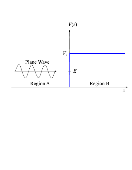
Figure 1: The relativistic quantum particles, described by a plane wave, before a potential barrier. The two regions A and B are also notated.

Equation (1) possesses regular solutions for the field $\varphi$ in Region A,

$$\varphi_{\textmd{A}}=e^{-\frac{i}{h}(Et-p.z)}+Re^{-\frac{i}{h}(Et+p.z)},$$ (4)

and Region B:

$$\varphi_{\textmd{B}}=Te^{\frac{i}{h}(Et-p^{\prime}.z)},$$ (5)

where $R$ and $T$ are two constants, related to the amplitude of the wave, and have to be identified.

1.1 Klein Paradox from Klein-Gordon equation

From equation (1), and also regarding the definitions for energy in (2) and (3), the total linear momentum can be written as

$$p=\sqrt{E^{2}-m^{2}c^{4}}$$ (6)

and

$$p^{\prime}=\pm\sqrt{(E-V)^{2}-m^{2}c^{4}}.$$ (7)

This could help us to categorize the total linear momentum with respect to the relations between the the total energy and the potential. The following cases arise:

• for weak potentials, where $V<E-mc^{2}$, the momentum $p^{\prime}$ would be real and only opts positive values.

• for an intermediate potential, $E-mc^{2}<V<E+mc^{2}$, $p^{\prime}$ takes imaginary values, providing unstable waves.

• when the potential is strong, i.e. $V>E+mc^{2}$, then $p^{\prime}$ is real and exhibits non-classical behaviors.

Now a question arises:

”How can we guarantee the charge current conservation?”

To deal with this question, we initially have to determine the values for $R$ and $T$ in (4) and (5). To do this, we are expected to apply the continuity condition for $\varphi$ and its derivative at $z=0$. In other words we set

$$\varphi_{A}|_{z=0}=\varphi_{B}|_{z=0},$$

$$\varphi^{\prime}_{A}|_{z=0}=\varphi^{\prime}_{B}|_{z=0}.$$

Therefore we get a system of linear equations.

$$1+R=T,$$

$$p(1-R)=Tp^{\prime}.$$ (8)

Solving the system in (1.1), gives the following values for $R$ and $T$:

$$R=\frac{p-p^{\prime}}{p+p^{\prime}},$$

$$T=\frac{2p}{p+p^{\prime}}.$$ (9)

Now we get back to the conservation of charge current. The charge current of a massive scalar field is defined by

$$\overrightarrow{j}=\frac{1}{2im}\Big{(}\varphi^{*}\overrightarrow{\nabla}\varphi-\varphi\overrightarrow{\nabla}\varphi^{*}\Big{)},$$ (10)

from which the current for the fields in (4) and (5) are derived as:

$${j_{A}}=\frac{h}{{2im}}\Big{(}{e^{\frac{i}{h}(Et-p.z)}}+{{{R}}^{{*}}}{}{e^{\frac{i}{h}(Et+p.z)}}\Big{)}\Big{(}\frac{{ip}}{h}{e^{\frac{{-i}}{h}(Et-p.z)}}-{{R}}\frac{{ip}}{h}{e^{\frac{{-i}}{h}(Et+p.z)}}\Big{)}$$

$$-\frac{h}{{2im}}\Big{(}{e^{\frac{{-i}}{h}(Et-p.z)}}+{{R}}{e^{\frac{{-i}}{h}(Et+p.z)}}\Big{)}\frac{{ip}}{h}\Big{(}-{e^{\frac{i}{h}(Et-p.z)}}+{{{R}}^{{*}}}{}{e^{\frac{i}{h}(Et+p.z)}}\Big{)},$$

$$<{j_{A}}>=\frac{p}{m}(1-{\left|R\right|^{2}}),$$ (11)

and

$${j_{B}}=\frac{h}{{2im}}\Big{[}{T^{*}}{e^{\frac{i}{h}(Et-p^{\prime*}.z)}}\frac{{ip^{\prime}}}{h}T{e^{\frac{{-i}}{h}(Et-p^{\prime}.z)}}-T{e^{\frac{{-i}}{h}(Et-p^{\prime}.z)}}(-\frac{{ip^{\prime}}}{h}){T^{*}}{e^{\frac{i}{h}(Et-p^{\prime*}.z)}}\Big{]},$$

$$\left\{\begin{array}[]{l}<{j_{B}}>=\frac{{p\prime}}{m}\left|{{T}}\right|^{2},{\rm{}}\,\,\,\,\,\,\,\,\,\,p^{\prime}\,\,{\rm{is\,\,real}}\\ \\ <{j_{B}}>=0,\,\,\,\,\,\,\,\,\,\,{\rm{}}p^{\prime}\,\,{\rm{is\,\,imaginary}}\end{array}\right..$$ (12)

Also one can define an average incident current, due to the linear momentum and mass of the field as

$$<j_{inc}>=\frac{p}{m}.$$ (13)

This will help us to investigate the ratios between $p$ and $p^{\prime}$, as functions of the reflection coefficient $R$, and the transmission coefficient $T$. Form (1.1) and the definitions in (1.1) and (1.1) we have:

$$|R|^{2}=\frac{|j_{A}-j_{inc}|}{j_{inc}}=\frac{|j_{R}|}{j_{inc}},$$

$$|T|^{2}=\frac{p}{p^{\prime}}\frac{j_{B}}{j_{inc}}.$$ (14)

And it is always expected that $R+T=1$. Note that, for an intermediate potential, $R=1,\,\,T=0$ and for a strong potential [2, 3]

$$R=\Big{(}\frac{p+|p^{\prime}|}{p-|p^{\prime}|}\Big{)}^{2},$$

$$T=-\frac{4p|p^{\prime}|}{(p-|p^{\prime}|)^{2}}.$$ (15)

One can observe that, for both cases the condition $R+T=1$ is satisfied. However, equation (1.1) asserts that $R>1$ and $T<0$; that is the reflected current is bigger than incident current, or the transmitted current is opposite in charge to incident current. This is what we know as the Klein paradox.

Historically, this result was obtained by Oskar Klein in 1929 [4] and since then, much effort has been devoted to this problem by stating that this unexpected reflected current is because of some extra particles which are being supplied by the potential, or this negative transmitted current is caused by another type of particles, possessing opposite charges [3, 5]. This explanation of Klein paradox was based on Klein-Gordon equation. Now let us have another approach through the Dirac equation.

1.2 Klein Paradox from Dirac equation

According Figure 1, one can consider two operating equations [6]. One for Region A ($z<0$):

$$(c\alpha\hat{p}+\beta mc^{2})\psi=E\psi,$$ (16)

and one for Region B ($z>0$):

$$(c\alpha\hat{p}+\beta mc^{2})\psi=(E-V_{0})\psi.$$ (17)

Also it would be possible to write down an incident wave function in region A.

$$\psi_{inc}=\alpha\left(\begin{array}[]{l}\,\,\,\,\,\,\,1\\ \,\,\,\,\,\,\,0\\ \frac{pc}{E+mc^{2}}\\ \,\,\,\,\,\,\,0\end{array}\right)e^{\frac{ipz}{\hbar}},$$ (18)

from which the reflected and the transmitted spinors are derived as

$$\psi_{R}=b\left(\begin{array}[]{l}\,\,\,\,\,\,\,1\\ \,\,\,\,\,\,\,0\\ \frac{-pc}{E+mc^{2}}\\ \,\,\,\,\,\,\,0\end{array}\right)e^{\frac{-ipz}{\hbar}}+b^{\prime}\left(\begin{array}[]{l}\,\,\,\,\,\,\,0\\ \,\,\,\,\,\,\,1\\ \,\,\,\,\,\,\,0\\ \frac{pc}{E+mc^{2}}\end{array}\right)e^{\frac{-ipz}{\hbar}},$$ (19)

$$\psi_{T}=d\left(\begin{array}[]{l}\,\,\,\,\,\,\,\,\,\,\,\,1\\ \,\,\,\,\,\,\,\,\,\,\,\,0\\ \frac{p^{\prime}c}{E-V_{0}+mc^{2}}\\ \end{array}\right)e^{\frac{ip^{\prime}z}{\hbar}}+d^{\prime}\left(\begin{array}[]{l}\,\,\,\,\,\,\,\,\,\,\,\,0\\ \,\,\,\,\,\,\,\,\,\,\,\,0\\ \frac{-p^{\prime}c}{E-V_{0}+mc^{2}}\end{array}\right)e^{\frac{ip^{\prime}z}{\hbar}}.$$ (20)

Note that,

$$p^{\prime}c=\sqrt{(V_{0}-E)^{2}-m^{2}c^{4}}.$$

Now consider the case of existence of a strong potential, $V_{0}>E+mc^{2}$. Same as in the previous subsection, applying the continuity condition on spinors at the boundary $\psi_{inc}+\psi_{R}=\psi_{T}$, we get [7]:

$$a+b=d,$$

$$b^{\prime}=d^{\prime},$$

$$\frac{pc}{E+mc^{2}}a-\frac{pc}{E+mc^{2}}b=\frac{-p^{\prime}c}{V_{0}-E-mc^{2}}d,$$

$$\frac{pc}{E+mc^{2}}b^{\prime}=\frac{p^{\prime}c}{V_{0}-E-mc^{2}}d^{\prime}.$$ (21)

Note that, the case $b^{\prime}=d^{\prime}=0$, means no spin flip.

In order to get back to the Klein paradox, let us write down the probability currents. The probability current can be written as

$$j(x)=c\psi^{\dagger}(x)\alpha_{3}\psi(x),$$ (22)

from which, using (1.2), we can derive the incidental, reflective and transmitted currents.

$$j_{inc}=aa^{*}\frac{2pc^{2}}{E+mc^{2}},$$

$$j_{R}=-bb^{*}\frac{2pc^{2}}{E+mc^{2}},$$

$$j_{T}=-dd^{*}\frac{2p^{\prime}c^{2}}{V_{0}-E-mc^{2}}.$$ (23)

This could help us to identify the reflection and transmission coefficients [3, 8].

$$R=\frac{j_{R}}{j_{inc}}=-\frac{bb^{*}}{aa^{*}}=\frac{(1+r)^{2}}{(1-r)^{2}},$$

$$T=\frac{j_{T}}{j_{inc}}=-\frac{4r}{(1-r)^{2}}.$$ (24)

Dealing with equation (1.2), one can see that for $r=\sqrt{\frac{(V_{0}-E+mc^{2})(E+mc^{2})}{(V_{0}-E-mc^{2})(E-mc^{2})}}$ we have $r\geq 1$. Once again, $R>1,\,\,\,T<0$; the reflected current is greater than the incident current. This means that we have been confronted the Klein paradox.

In this paper we concern about the mentioned paradox, however from another viewpoint, namely from Krein space quantization, which will be introduced in the next section. An important idea to surmount Klein paradox is that it is supposed that the potential energy increases the negative energy of the electron, to a positive energy state, creating a positive hole (positron) behind it. The hole is attracted towards the potential while the electron is repelled far from it. This process is stimulated by the incoming electron (see Figure 2). However, in this article we suggest that we could keep the negative energies as viable energies. Through Krein quantization approach, we put that these negative energies were possible to be included in our calculations and just like what was asserted, they essentially could be regarded as un-physical particles and antiparticles. Having them, the energy conservation is also guaranteed. First of all, let us have an overview on Krein quantization.

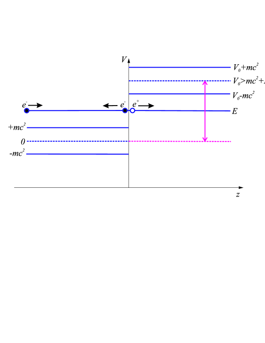
Figure 2: The incoming negative electron can be regarded as a reflected negative electron with same energy, and a transmitted positron.

2 Krein Quantization

As it was discussed in the previous section, there would be some unexpected negative energies in transmitted fermions trough the barrier. Initially, Dirac proposed to keep these negative states. After that, much efforts have been devoted to construct a viable theory for appropriate interpretations of negative energies. What we are concerning about here, is a new method, called Krein quantum field theory, being able to use the so-called negative energies. Krein quantization is based on removing the divergences, caused by singularities in Green’s function [9].

Let us begin with a scalar field quantization in the form [10, 11, 12, 13]

$$\phi(x)=\frac{1}{\sqrt{2}}\Big{[}\phi_{p}(x)+\phi_{n}(x)\Big{]},$$ (25)

where

$$\phi_{p}(x)=\int d^{3}\overrightarrow{k}\,\,\Big{[}a(\overrightarrow{k})u_{p}(\overrightarrow{k},x)+a^{\dagger}(\overrightarrow{k})u^{*}_{p}(\overrightarrow{k},x)\Big{]},$$

and

$$\phi_{n}(x)=\int d^{3}\overrightarrow{k}\,\,\Big{[}b(\overrightarrow{k})u_{n}(\overrightarrow{k},x)+b^{\dagger}(\overrightarrow{k})u^{*}_{n}(\overrightarrow{k},x)\Big{]}.$$

Here, the lower the indices $p$ and $n$, respectively referring to the positive and negative states (or modes). The positive mode is the usual scalar field and the negative one, which here we are about to consider, would be the regularization field. As we mentioned above, the divergences in quantum field theory are caused by the Green’s function singularities. This Green’s function is defined as a time-ordered product [14, 15, 16].

$$iG_{T}(\overrightarrow{x},\overrightarrow{x}^{\prime})=<0|T\phi(x)\phi(x^{\prime})|0>=\textmd{Re}[G_{F}(\overrightarrow{x},\overrightarrow{x}^{\prime})],$$ (26)

where $G_{F}(\overrightarrow{x},\overrightarrow{x}^{\prime})$ is the Feynman Green function [13]. According to this, the time-ordered product propagator in the Feynman gauge for the vector field in Krein space is given by [13, 23]:

$$<D_{\mu\nu}^{T}(x,x^{\prime})>=-\eta_{\mu\nu}<G_{T}(x,x^{\prime})>.$$ (27)

The most essential notion of Krein quantization would be its impact on the solutions of Dirac equation. The Dirac field in Krein space is written in the following form (for a detailed discussion see [9]):

$$\Phi_{\textmd{D-K}}(\overrightarrow{x})=\frac{1}{\sqrt{2}}\int d^{3}\overrightarrow{k}\sum_{i=1,2}\Big{[}(b_{\overrightarrow{k}i}+c^{\dagger}_{\overrightarrow{k}i})\mathbf{P}^{i}(\overrightarrow{k},\overrightarrow{x})+(d^{\dagger}_{\overrightarrow{k}i}+a_{\overrightarrow{k}i})\mathbf{N}^{i}(\overrightarrow{k},\overrightarrow{x})\Big{]},$$ (28)

in which the the modes $\mathbf{P}^{i}$ and $\mathbf{N}^{i}$ are defined as

$$\mathbf{P}^{i}(\overrightarrow{k},\overrightarrow{x})=\sqrt{\frac{m}{(2\pi)^{3}\omega_{\overrightarrow{k}}}}\,\,\mathbf{p}^{i}(\overrightarrow{k})e^{-i\overrightarrow{k}.\overrightarrow{x}}$$ (29)

for positive energies, and

$$\mathbf{N}^{i}(\overrightarrow{k},\overrightarrow{x})=\sqrt{\frac{m}{(2\pi)^{3}\omega_{\overrightarrow{k}}}}\,\,\mathbf{n}^{i}(\overrightarrow{k})e^{i\overrightarrow{k}.\overrightarrow{x}}$$ (30)

for negative energies. Here it is necessary to indicate the notions of the operators in (28). We introduce [17]

• $b$: is the annihilation operator of one-particle (or one-antiparticle) state with positive energy.

• $c^{\dagger}$: is the creation operator of one-particle (or one-antiparticle) state with positive energy.

• $d^{\dagger}$: is the creation operator of one-particle (or one-antiparticle) state with negative energy.

• $a$: is the annihilation operator of one-particle (or one-antiparticle) state with negative energy.

Also the time-ordered propagator is defined as

$$S_{T}(\overrightarrow{x},\overrightarrow{x}^{\prime})=(i\not\partial+m)G_{T}(\overrightarrow{x},\overrightarrow{x}^{\prime}),$$ (31)

in which the Green function $G_{T}(\overrightarrow{x},\overrightarrow{x}^{\prime})$ has been presented in (26). These two modes would be the key point in our approach to discuss the Klein paradox, which we will deal with in the next section. This suggestion is based on this belief that, although have not been correlated to physical concepts, the negative norm states are still appearing in the mathematical procedures, together with the positive energies; as we will see in the next section, they have an important impact on the results. Therefore, the un-physical (or virtual) particles, may appear to have physical meanings in the future, however, we are dealing with the mathematical results and according to Feynman’s phrase, we are not ”hiding the rushes under the carpet”.

Through Krein quantization, we are asserting that solutions are corresponding to the particles and antiparticles of positive energies (physical particles of positive states) and those of negative energies (un-physical particles of negative stats). Therefore, in our approach, we shall maintain all 4 solutions, in order to having all physical and un-physical particles and antiparticles. [10, 11, 14, 18].

As stated by Dirac, ”negative energies and probabilities should not be considered as nonsense. They are well-defined concepts mathematically, like a negative sum of money, since the equations which express the important properties of energies and probabilities, can still be used when they are negative. Thus, negative energies and probabilities should be considered simply as things which do not appear in experimental results. The physical interpretation of relativistic theory involves these things and is thus in contradiction with experiment. We therefore, have to consider ways of modifying or supplementing this interpretation.” [19, 20].

3 Explaining Klein Paradox through Krein Quantization

Maintaining an overlook on Klein paradox via Klein-Gordon and Dirac solutions, now let us present a recently proposed explanation for this paradox, which is based on Krein quantization. In section one, it was asserted that among the electrons of positive energies, which are coming down onto the potential barrier, some are being reflected from the barrier (travelling along $-z$ direction), and some could be assumed to be the passing positrons travelling along $+z$ direction (see Figure 2). However, a crucial point has to be the reflected electrons of negative energy, and this is what we are about to consider in our new approach. According to Dirac’s equation, there are four sets of solutions available, including up and down spin electrons of positive energy, and up and down spin electrons of negative energy. In all cases, which we have dealt with, the incidental electron current (Region A in Figure 1) always possesses positive energies (having either up or down spins). This means that the so-called negative energies have been ruled out.

The technical point in Krein quantization approach, is keeping all the sets of solutions, even for negative energies. Let us see what this procedure provides us. Concerning with the electrons with negative energies, one can discover that the reflected and transmitted electrons are covering all the incidental current, and this means that the transmitted positrons (or transmitted positrons of positive energy) are no longer necessary to be considered to surmount the problem of negative current density. Strictly speaking, what we are going to put here, is that problems like backwardly moving electrons of negative current which are leading to Klein paradox, are indeed arising from the fact that we have ignored the electrons of negative energies. This lack of initial data, will command us to consider some reflected positrons and transmitted electrons of positive energy. However if we had maintained all the Dirac’s solutions, we could have protected our selves of this explanation, since this leads to an equality between the incidental and the total reflected currents, for either of the electrons and the positrons (see Figure 3). This means that, we could overcome the Klein paradox. In other words, through this approach, no paradox will remain to be explained.

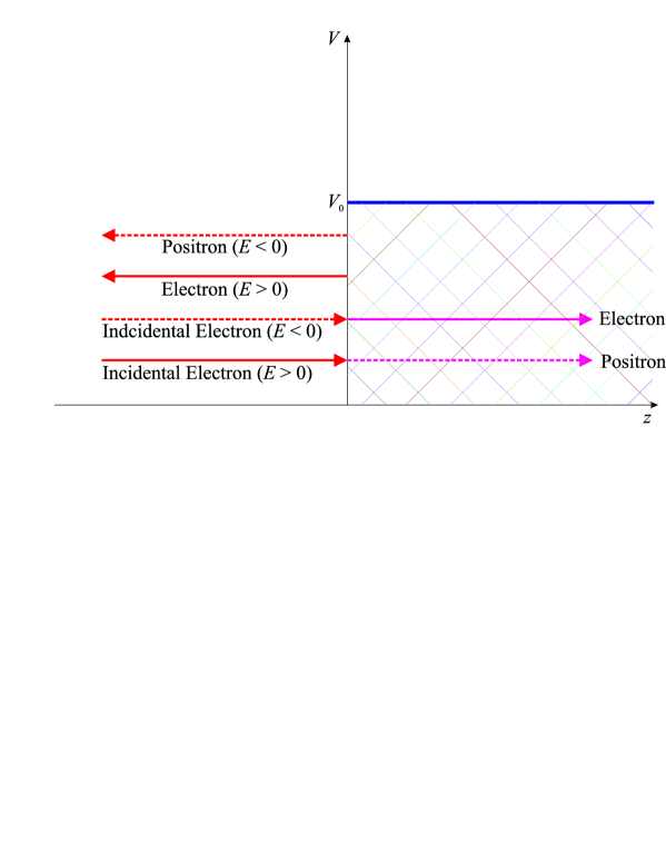
Figure 3: The incidental electrons or positrons having positive and negative energies.

To prove our recent statements, recall the parameter $r$ related to the reflected current from equation (1.2). As it was mentioned in section one, we have

$$r=\sqrt{\frac{(E-V_{0}-mc^{2})(E+mc^{2})}{(E-V_{0}+mc^{2})(E-mc^{2})}}$$ (32)

for which we have $r>1$. Letting the negative modes to contribute in our calculations, we define another parameter, namely $r^{\prime}$, to retain the correlations between the so-called negative states and the reflected current. If $E<0$, then the negative states choose

$$r^{\prime}=\sqrt{\frac{(-E-V_{0}-mc^{2})(-E+mc^{2})}{(-E-V_{0}+mc^{2})(-E-mc^{2})}},$$ (33)

as the reflection parameter for electrons of negative energies. Note that

$$rr^{\prime}=k,\,\,\,\,\,\,\,\,\,\,k>1.$$

Having this, we can investigate the ratios between the incidental, reflected and transmitted currents; i.e. $\frac{|j^{\prime}_{T}|}{|j^{\prime}_{inc}|}$ and $\frac{|j^{\prime}_{R}|}{|j^{\prime}_{inc}|}$. Equation (33) yields

$$-E-V_{0}+mc^{2}<0\,\,\,\,\,\,\,\,\,\,\,\,\,\textmd{or}\,\,\,\,\,\,\,\,\,\,\,\,-E<V_{0}-mc^{2}.$$

Multiplying $r$ and $r^{\prime}$ from (32) and (33), we get

$$rr^{\prime}=\sqrt{\frac{(E-V_{0}-mc^{2})(E+V_{0}+mc^{2})}{(E-V_{0}+mc^{2})(E+V_{0}-mc^{2})}}.$$ (34)

Simplifications give

$$k=\sqrt{\frac{E^{2}-(V_{0}+mc^{2})^{2}}{E^{2}-(V_{0}-mc^{2})^{2}}}.$$ (35)

It turns out that always $k>1$ and for $V_{0}\rightarrow\infty$, $k\rightarrow 1$. Now having $r^{\prime}$ and $k$, we can derive same relations for density currents as they are in (1.2), for the negative modes.

$$R^{\prime}=\frac{|j^{\prime}_{R}|}{|j^{\prime}_{inc}|}=\frac{(1+r^{\prime})^{2}}{(1-r^{\prime})^{2}}=\frac{\Big{(}1+\frac{k}{r}\Big{)}^{2}}{\Big{(}1-\frac{k}{r}\Big{)}^{2}}=\frac{(k+r)^{2}}{(k-r)^{2}},$$

$$T^{\prime}=\frac{|j^{\prime}_{T}|}{|j^{\prime}_{inc}|}=\frac{4r^{\prime}}{(1-r^{\prime})^{2}}=\frac{4\Big{(}\frac{k}{r}\Big{)}}{\Big{(}1-\frac{k}{r}\Big{)}^{2}}=\frac{4kr}{(k-r)^{2}}.$$ (36)

Now to advocate our previously claim, that having all the modes could give us equal numbers of reflected and transmitted electrons and positrons, we consider we have $M$ to be the total number of the reflected and transmitted electrons (of both positive and negative energies), and $N$ to be the total number of the reflected and transmitted positrons (of both positive and negative energies). Using (1.2) and the parameters in (3), we get

$$R|_{E>0}+T^{\prime}|_{E<0}=\Big{(}\frac{1+r}{1-r}\Big{)}^{2}+\frac{4kr}{(k-r)^{2}}=M,$$

$$R^{\prime}|_{E<0}+T|_{E>0}=\Big{(}\frac{k+r}{k-r}\Big{)}^{2}+\frac{4r}{(1-r)^{2}}=N.$$ (37)

The only task remaining is to prove $M=N$. The denominators for the both relations in (3) are the same, therefore we shall switch to the numerators. We have

$$\textmd{the numerator of $M$}=k^{2}+r^{3}+2kr+k^{2}r^{2}+r^{4}+2kr^{3}+2k^{2}r+2r^{3}-12kr^{2},$$

$$\textmd{the numerator of $N$}=k^{2}+r^{3}+2kr+k^{2}r^{2}+r^{4}+2kr^{3}+2k^{2}r+2r^{3}-12kr^{2}.$$ (38)

And this is what we were looking for; same values for the total reflected and transmitted numbers, for both electrons and positrons.

4 Conclusion

In this article we initially stated the Klein paradox, were the anomalous and unexpected numbers of reflected electrons from a potential barrier, has itself begun to appear as an obstacle beyond physicists. Since Dirac himself had essentially omitted the negative modes in his solutions, the most recognized explanation for such paradox was the consideration of backwardly moving electrons and transmitting positrons with positive energy. This explanation and the similar ones, have been criticized and under consideration for many years. Some physicists support theories like them, however these are just legitimizations. In this article, we are endeavoring to get rid of the paradox itself. We believe that by maintaining the negative modes (or negative energies), it would be possible to regain the total incidental current and the exact number of electrons, without confronting strange backward travelling electrons. Our progress was based on the Krein quantization, concerning all four of Dirac’s solutions. What we are dealing with, is that we can validate this possibility, that the negative states could be considered as viable energies.

Here we must note that, our approach to the quantum theory of fields (namely Krein quantization), still exposes a mathematical picture. Through this mathematical approach, some important physical phenomena, like Casimir effect, have been retreated [21]. Briefly speaking, we try to remove the divergences, caused by the QFT Green’s function, by considering all four solutions of Dirac field equation. This seems to be of some physical applications and in this case, removing the Klein paradox.

While the Krein quantization method, is a seemingly totally mathematical one, some physicist are endeavoring to bring up its probable physical implications (see [22, 23, 24]). However, despite these efforts, the proper physical picture of Krein quantization is not still clear. Therefore, unless this method has been used in order to explaining the QCD concepts and been compared with the ghost field results, the appropriate physical picture will not be clarified.

Nevertheless the negative energies in quantum physics have not been related to real physical concepts, however the results in this paper, may open doors for further considerations, and this is what we were looking for.

- [1] Kaku M. Quantum Field Theory: A Modern Introduction. Oxford University Press, Oxford, 1993
- [2] Dirac P A M. Proc. Roy. Soc., 1928, 117: 612
- [3] Calogeracos A, Dombey N. Contemp. Phys., 1999, 40: 313-321
- [4] Klein O. Zeitschrift für Physik, 1929 53 (3 4)
- [5] Dombey N, Calogeracos A. Physics Reports, 1999, 315 (1 3): 41
- [6] Robinson T R. American Journal of Physics, 2012, 80 (2): 141
- [7] Katsnelson M I, Novoselov K S, Geim A K. Nature Physics, 2006, 2 (9): 620. arXiv: cond-mat/0604323
- [8] Pendry B J. Science, 2007, 315 (5816): 1226
- [9] Payandeh F, Mehrafarin M, Takook M V. Sci. Chin. G: Phys. Mech. Astron., 2009, 52: 212
- [10] Gazeau J-P, Renaud J, Takook M V. Class. Quant. Grav., 2000, 17: 1415
- [11] Takook M V. Mod. Phys. Lett. A, 2001, 16: 1691
- [12] Rouhani S, Takook M V. Int. J. Theor. Phys., 2009, 48: 2740
- [13] Payandeh F, Moghaddam Z Gh, Fathi M. Fortschr. Phys., 2012, 60, No. 9-10: 1086
- [14] Takook M V. Int. J. Mod. Phys. E, 2002, 11: 509
- [15] Rouhani S, Takook M V. arXiv: gr-qc/0607027
- [16] Payandeh F, Mehrafarin M, S. Rouhani S et al. Ukr. J. Phys. V, 2008, 53: N 12
- [17] Payandeh F. Rev. Cub. F sica, 2009, 26 No.2B: 232
- [18] Garidi T, Huguet E, Renaud J. J. Phys. A, 2005, 38: 245
- [19] Dirac P A M. Bakerian Lecture Proc. Roy. Soc. Lond. A, 1942, 180: 1
- [20] Dirac P A M. Nobel Lecture, December 12, 1933
- [21] Payandeh F, ISRN High Energy Phys., 2012, 2012: 714823
- [22] Refaei A, Takook M V. Phys. Lett. B, 2011, 704: 326
- [23] Refaei A, Takook M V. Mod. Phys. Lett. A, 2011, 26: 31
- [24] Forghan B, Takook M V, Zarei A. Annals of Physics, 2012, 327: 2388