State transition induced by self-steepening and self phase-modulation

Abstract

We present a rational solution for a mixed nonlinear Schrödinger (MNLS) equation. This solution has two free parameters $a$ and $b$ representing the contributions of self-steepening and self phase-modulation (SPM) of an associated physical system. It describes five soliton states: a paired bright-bright soliton, single soliton, a paired bright-grey soliton, a paired bright-black soliton, and a rogue wave state. We show that the transition among these five states is induced by self-steepening and SPM through tuning the values of $a$ and $b$. This is a unique and potentially fundamentally important phenomenon in a physical system described by the MNLS equation.
KEYWORDS: Mixed nonlinear Schrödinger equation, state transfer, Alfvén wave, ultra-short light pulse, rational solution.

Introduction. The mixed nonlinear Schrödinger (MNLS) equation KMio ,

$$q_{t}-iq_{xx}+a(q^{\ast}q^{2})_{x}+ibq^{\ast}q^{2}=0,$$ (1)

has been derived by the modified reductive perturbation method to describe the propagation of e.g. the Alfvén waves with small but finite amplitude along the magnetic field in the cold plasma approximation widely applicable in solar, solar-terrestrial, space and astrophysicsmedvedev ; sulem . Later it has been shown Tzoar ; Anderson ; Zabolotskii that the MNLS equation also provides an accurate modelling of ultra-short light pulse propagation in optical fibers. In eq. (1) the complex quantity $q$ represents the magnetic field perturbation in the case of Alfvén waves, and the electrical field envelope in the case of waves in optical fibres. The asterisk denotes complex conjugate, $a$ and $b$ are two non-negative constants determined by the unperturbed state, and the subscript $x$ ($t$) denotes the partial derivative with respect to the spatial coordinate $x$ (time $t$). The MNLS equation reduces to the Nonlinear Schrödinger (NLS) equation when $a=0$, and to the Derivative Nonlinear Schrödinger (DNLS) equation when $b=0$. Because the MNLS equation is applicable even in the case where the lengths of the envelope wave and the carrier wave are comparable KMio , it is more general than the nonlinear Schrödinger equation in the modelling of waves in optical fibres. The last three terms in eq. (1) describe the group velocity dispersion (GVD), self-steepening and self phase-modulation (SPM), respectively.

The Lax pair for the MNLS equation provides the mathematical basis for the solvability of this equation by the inverse scattering method and Darboux transformation (DT), the latter being defined by the Wadati-Konno-Ichikawa (WKI) spectral problem and the first non-trivial flow MikiWadati1

$$\begin{array}[]{ll}\partial_{x}\psi=(-aJ\lambda^{2}+Q_{1}\lambda+Q_{0})\psi\equiv U\psi,\vspace*{2mm}\\ \partial_{t}\psi=(-2a^{2}J\lambda^{4}+V_{3}\lambda^{3}+V_{2}\lambda^{2}+V_{1}\lambda+V_{0})\psi\equiv V\psi,\end{array}$$

with the reduction condition $r=-q^{\ast}$. Here the complex quantity $\lambda$ is the eigenvalue (or spectral parameter), and $\psi=(\phi,\varphi)^{T}$ is the eigenfunction associated with $\lambda$. The superscript $T$ denotes transposition. There are also other methods to show the integrability of the MNLS equation and to obtain its exact solutions AKundu ; Seenuvasakumaran ; QingDing ; Kundu . Various types of solutions of the MNLS equation, including a soliton and a breather have already been obtained in TKawata ; Chowdhury ; mihalache ; Doktorov2 ; Rangwala ; OCWrigh ; TiechengXia ; HaiQiangZhang ; Shanliang ; MinLi . The decay of soliton solution for a perturbed MNLS system has been demonstrated numerically serkindecay . Small perturbations of the MNLS equation have been studied either by a direct method perturbation , or using the inverse scattering transform Shchesnovich ; VMLashkin .

Up to now, all known solutions of the MNLS equation represent rather common nonlinear wave solutions, like solitons and breathers. These are similar corresponding ones to their ancestors — the NLS and DNLS equation, so they do not describe any specific properties of either the Alfvén waves in magnetised plasmas, or ultrashort light pulses in optical fibres. Thus, it is a long-standing problem to find unique phenomena related to the simultaneous effects of self-steepening and SPM that can be described by the explicit analytical solutions of the MNLS equation.

In this letter we present novel rational solutions of the MNLS equation. These solutions describe five states of the associated systems: a paired bright-bright soliton state, a single soliton state, a paired bright-grey soliton state, a paired bright-dark soliton state, and a rogue wave state. We also show that the transition between these five states is induced by the self-steepening and SPM through tuning the values of $a$ and $b$ determined by the physical properties of the background state.

Analytical form of rational solution. By the one-fold DT and Taylor-expansion, according to a similar procedure demonstrated by he2 ; xuhe ; xxuhe ; taohe ; hexup for constructing the rational rogue wave (RW) of the NLS, DNLS, Hirota and NLS-Maxwell-Bloch equations, a novel rational solution of the MNLS equation is given as follows

$${q^{[1]}}=-\exp[i(-x-tb-t+ta)]\dfrac{r_{1}r_{2}}{{r_{1}^{*}}^{2}},$$ (2)

$$r_{1} \mbox{}=X+1+2ia[(3a-2)t-x],$$

$$r_{2} \mbox{}=X-3+2i[(-6a+3a^{2}+4b)t-ax],$$

$$X \mbox{}=2(a-b)[(-2b+3a^{2}\mbox{}-6a+4)t^{2}\mbox{}+4(1-a)xt+x^{2}].$$

We omit the tedious calculation of this solution. The validity of this solution has been confirmed by symbolic computation. By letting $x\rightarrow{\infty}$ and $t\rightarrow{\infty}$ it is easy to show that $|q^{[1]}|^{2}\rightarrow 1$, and $|q^{[1]}|^{2}(0,0)=9$. So, $q^{[1]}$ denotes a rational solution on a non-zero background with a unit height. This is a new and wide class of solutions for the MNLS equation because it can encompass five kinds of solution.

Transition between five states. We are now in the position to explore the properties of $q^{[1]}$ with more details. The trajectory of $|q^{[1]}|^{2}$ in the $(x,t)$-plane is defined by the location of the ridge (or vale) of its profile. A good approximation of the trajectory for $|q^{[1]}|^{2}$ is given through a simple equation $X+1=0$ in general. By a straightforward but tedious calculation of the stationary point of $|q^{[1]}|^{2}$ in the ($x,t$)-plane we find, that, $q^{[1]}$ describes five solutions associated with five regions in the upper-right quadrant on the ($a,b$)-plane (see Figure 1), as follows

I ( $b>a$). There is only one saddle point of $|q^{[1]}|^{2}$ at $(0,0)$, and there are two simultaneous trajectories $X_{1}$ and $X_{2}$ on the ($x,t$)-plane. Note that the trajectories are not two straight lines as usual in the case of double solitons. If the height of soliton $|q^{[1]}|^{2}$ is increasing as it evolves along $X_{1}$, then it will decrease as it evolves on $X_{2}$. The asymptotic height of $|q^{[1]}|^{2}$ is $H_{1}=H_{1}(a,b)$ as $t=-\infty$, and $H_{2}=H_{2}(a,b)$ as $t=+\infty$ on $X_{1}$; $|q^{[1]}|^{2}$ approaches to $H_{2}$ as $t=-\infty$ and to $H_{2}$ as $t=+\infty$ on $X_{2}$. Thus, when $(a,b)\in$ region I, $q^{[1]}$ is called a paired bright-bright soliton because $H_{2}>H_{1}>1$ and the appearance of two peaks (i.e. an increasing peak and a decreasing one). Obviously, there exists energy exchange between the two bright peaks propagating along $X_{1}$ and $X_{2}$ in accordance with the energy conservation. In particular, the distance between the two peaks is proportional to $\sqrt{\delta_{1}t^{2}+\delta_{2}}$ in contrast to a linear function of $t$ for the known two peaks in the case of a double soliton. Here $\delta_{1}$ and $\delta_{2}$ are two real functions of $a$ and $b$.

II ($b=a$). $|q^{[1]}|^{2}$ takes its maximum value 9 when ($x,t$) is on the line $x=(-2+3a)t$. This line is also the trajectory of $|q^{[1]}|^{2}$. This is a single soliton solution.

III ($a>b>\max[0,a-\frac{3}{8}a^{2}]$). There is only one extremum of $|q^{[1]}|^{2}$ at ($0,0$) on the ($x,t$)-plane. Most features of the obtained solution are similar to those of region I except $H_{2}>1>H_{1}>0$. Thus, in this region, $q^{[1]}$ is called a paired bright-grey soliton. Note that $a-\frac{3}{8}a^{2}<0$ if $a>\frac{8}{3}$.

IV ($b=a-\frac{3}{8}a^{2}$, $a\in[0,\frac{8}{3}]$). There is only one extremum of $|q^{[1]}|^{2}$ at ($0,0$) in the ($x,t$)-plane. The solution resembles that of region III except that $H_{2}>1>H_{1}\geq 0$. Thus, in region IV of the ($a,b$)-plane, $q^{[1]}$ is called a paired bright-dark soliton.

V ($0<b<a-\frac{3}{8}a^{2}$). For $|q^{[1]}|^{2}$, there is only one maximum at (0,0), where $|q^{[1]}|^{2}=9$, and two minima, where $|q^{[1]}|^{2}=0$. The two minima are located with the coordinates given by

$$\begin{array}[]{ll}\displaystyle x=\mp\dfrac{-6a+3a^{2}+4b}{a-b}\sqrt{\dfrac{3}{32((a-\frac{3}{8}a^{2})-b)}},\vspace*{2mm}\\ \displaystyle t=\pm\dfrac{a}{a-b}\sqrt{\dfrac{3}{32((a-\frac{3}{8}a^{2})-b)}}\end{array}$$

at the points in the $(x,t)$-plane. When $(a,b)$ is region V, $|q^{[1]}|^{2}$ is localised both in the $x$ and $t$ direction, and thus $q^{[1]}$ is a rogue wave solution of the MNLS equation.

The main difference between the grey and dark soliton is that the minimum of the solution may or may not reach zero ablowitz1 for the grey one.

For a physical system modelled by the MNLS equation, each solution presented above gives a particular phase state. So, it is rather interesting to observe in Figure 1 that there exists the state transition induced by tuning the self-steepening and SPM, which can be realised by adjusting the values of $a$ and $b$. For example, by setting $a=\frac{1}{2}$ and varying $b$, the system will evolve consecutively through a paired bright-bright, a single, a paired bright-grey, a paired bright-dark soliton states, and the rogue wave state as $b$ decreases from a value larger than $\frac{1}{2}$ to one that is smaller than $\frac{13}{32}$. Moreover, for a given $b>b_{c}(=\frac{2}{3})$, the system passes through the first three (i.e. I-III) states as $a$ increases from $zero$ to a sufficiently large value; for $b=b_{c}$, the system now passes through the first four (i.e. I-IV) states, and it passes through the paired bright-grey soliton state twice; finally, for $b<b_{c}$, the system passes through all five states and will be in paired bright-grey and paired bright-dark soliton states twice. This newly discovered unique state transition phenomenon is not described by the rational solutions of the NLS and DNLS equations because they do not describe two different nonlinear effects simultaneously. Thus, we have now solved the long-standing problem mentioned in the Introduction.

Particular cases. In what follows we use two methods to visualise function $|q^{[1]}|^{2}$. The first method consists of plotting the profile of $|q^{[1]}|^{2}$ which is the graph of this function of two variables in three dimensions. The second method is similar to drawing the level lines of this function, however, not using the lines but various colours instead. The figure obtained this way is called the density plot of the function $|q^{[1]}|^{2}$. In this plot each colour corresponds to a definite value of $|q^{[1]}|^{2}$.

To illustrate the general results we investigate the evolution of the rational solution for a fixed $a=\frac{1}{2}$ and varying $b$. In Figure 2 the profile (left panel) and density plot (right panel) of $|q^{[1]}|^{2}$ are shown for a paired bright-bright soliton with $b=1$. In Figure 3 the energy exchange (left panel) for two peaks along the two trajectories (right panel) is plotted. The limit heights in Figures 2 and 3 are $H_{2}=21+4\sqrt{5}\approx 29.9$ and $H_{1}=21-4\sqrt{5}\approx 12.1$. Note that the height of the background in Figure 2 is equal to 1. On the right panel of Figure 3, the explicit equations of trajectories $X_{1}$ (red line) and $X_{2}$ (green line) are $-t+\frac{1}{2}\sqrt{5t^{2}+4}=x$ and $-t-\frac{1}{2}\sqrt{5t^{2}+4}=x$, respectively. The distance between the two peaks at a given time is $\sqrt{5t^{2}+4}$ unlike the case of the two peaks in a double soliton solution. It is straightforward to see in Figure 3 (left panel) that the energy is transmitted gradually from a bright soliton (green line) moving along $X_{2}$ to the other bright soliton (red line) moving along $X_{1}$. The reflective symmetry of Figure 3 (left panel) refers to the energy conservation . By comparing Figure 2 (right panel) with Figure 3 (right panel), we can now see that the trajectory gives a very good approximation of the ridge location in the profile of $|q^{[1]}|^{2}$. Setting $a=b=\frac{1}{2}$, so that ($a,b$) is in region II, we obtain $|q^{[1]}|^{2}=\dfrac{36+(t+2x)^{2}}{4+(t+2x)^{2}}$, which is a single soliton with the height 9 and the exact trajectory $t+2x=0$. We do not show the profile in this case because it is a standard soliton.

In region III, by setting $b=\frac{9}{20}$, we obtain a paired bright-grey soliton. Its profile is plotted in Figure 4 (left panel). The limit height of the bright soliton is $H_{2}=\frac{8-\sqrt{15}}{20-5\sqrt{15}}\approx 6.5$, and the limit height of the grey soliton is $H_{1}=\frac{8+\sqrt{15}}{20+5\sqrt{15}}\approx 0.3$. The $X_{1}$ (red line) and $X_{2}$ (green line) in Figure 4 (right panel) give good approximation of the trajectories for $|t|>8$.

Let us set $a=\frac{1}{2}$ and $b=a-\frac{3}{8}a^{2}\approx 0.41$, the point $(a,b)$ is now in region IV, and the rational solution describes a bright-dark soliton. The profile of this solutions is shown in Figure 5 (left panel). The limit heights are $H_{2}=4$ for the bright soliton and $H_{1}=0$ for the dark one. The trajectories $X_{1}$ and $X_{2}$ are shown on the left panel of Figure 5 by the red and green lines, respectively. The analysis of the two solutions corresponding to the bright-grey and bright-dark solitons shows that: (i) There is energy exchange between the bright and grey (dark) solitons; (ii) the bright soliton is transformed into a grey (dark) one because its energy is lost during the interaction, while the grey (dark) soliton is transformed into a bright one for $t\gg 1$.

Finally, by setting $a=\frac{1}{2}$ and $b=\frac{1}{3}$, we put the point $(a,b)$ in region V. In this case the rational solution describes the first-order rogue wave, which is plotted in Figure 6.

Conclusions. We have presented a range of new types of rational solution of the MNLS equation that describe the propagation of e.g. Alfvén waves in magnetised plasmas and the femtosecond light pulses in optical fibres. The obtained solutions have two free parameters, $a$ and $b$, representing the contributions of self-steepening and self phase-modulation, and, depending on the values of these parameters, these solutions describes five types of novel solitons corresponding to five states of an associated physical system. These solutions are: A paired bright-bright, single, paired bright-grey, and a paired bright-dark soliton, and a rogue wave. We have found that the state transition among these five states is induced by tuning the effects of self-steepening and SPM. We urge that this novel phenomenon may be observed in laboratory or in magnetised plasma in nature in order to demonstrate an intricate balance between the effects of self-steepening and SPM in an associated physical system. Furthermore, because of the recent discovery of Alfvén waves (see alfven ; robertus1 and references therein) in the magnetised solar atmosphere, it is now paramount interest to find these novel states and the state transfer in space plasmas, and, to establish their connection with the long-standing coronal heating problem clare ; robertus2 ; robertus3 ; morton .

Finally, we discuss briefly the novelty of the solution describing the paired bright-bright soliton. Three of its characteristics, i.e. the existence of two peaks, decreasing or increasing amplitude, and the curved trajectories, are essentially different from the similar characteristics of the recently found solition solutions that include an explode-decay soliton nakamura , a two-peak soliton satsuma ; li , a W-shape soliton zhou2 , a dark-in-bright soliton Kevrekidis ; prosezian , a rogue wave peregrine and a two-peak rogue wave he2012 ; akhmedievpre2012 , in addition to the well-known classical soliton, breather, and kink. In particular, the paired bright-bright soliton is not a travelling wave. The non-autonomous solitons serkin1 ; jvv1 ; jvv2 ; heli2011 have the properties similar to those of the paired bright-bright soliton but only when they are solutions to the variable coefficient soliton equations. This discussion can also be applied to the paired bright-grey and bright-dark soliton solutions.
Acknowledgements This work is supported by the NSF of China Grant No.10971109 and 11271210, and K.C. Wong Magna Fund in Ningbo University. J. He is also supported by the Natural Science Foundation of Ningbo, Grant No. 2011A610179. R.E. acknowledges M. Kéray for patient encouragement and is also grateful to NSF, Hungary (OTKA, Ref. No. K83133) for the support received. J. He thank sincerely Prof. A.S. Fokas for arranging the visit to Cambridge University in 2012-2013 and for many useful discussions .

Fig. 1: (Colour online) Five regions in the upper-right quadrant on the ($a,b$)-plane. In each region, $q^{[1]}$ gives a new kind of solution for the MNLS equation. The straight green line is $a=b$, the red curve is defined by $b=a-\frac{3}{8}a^{2}$ for $a\leq\frac{8}{3}$, $b=0$ for $a\geq\frac{8}{3}$.

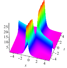
Fig. 2: (Colour online) The profile (left) and density plot (right) for a paired bright-bright soliton.

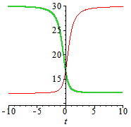
Fig. 3: (Colour online) Left: The energy transmission from a bright soliton (green line) to another one (red line). Right: The trajectories of the solitons, $X_{2}$ (green line) and $X_{1}$ (red line).

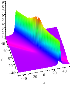
Fig. 4: (Colour online) The paired bright-grey soliton (left) and its trajectories (right).

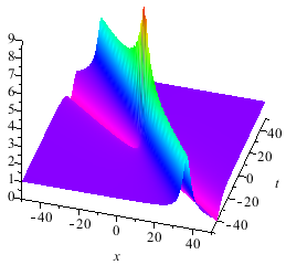
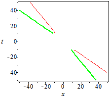
Fig. 5: (Colour online) The paired bright-black soliton (left) and its trajectories (right).

Fig. 6: (Colour online) The first-order rogue wave (left) and its density plot (right).

References

- (1) K. Mio, T. Ogino, K. Minami and S. Takeda, J. Phys. Soc. Jpn. 41(1976), 265-271.
- (2) M. V. Medvedev, P. H. Diamond, V. I Shevchenko and V. L. Galinsky Phys. Rev. Lett. 78(1997), 4934-4937.
- (3) D. Laveder, T. Passot, P.L. Sulem, Phys. Lett. A377(2013),1535-1441.
- (4) N. Tzoar and M Jain, Phys. Rev. A 23(1981),1266-1270.
- (5) D. Anderson and M. Lisak, Phys.Rev. A 27(1983),1393-1398
- (6) A. A. Zabolotskii,Phys. Lett. A. 124(1987), 500-502.
- (7) M. Wadati, K. Konno and Y.H. Ichikawa, J. Phys. Soc. Jpn. 46(1979), 1965-1966.
- (8) A. Kundu, J. Math. Phys. 25(1984),3433-3438.
- (9) K. Porsezian, P. Seenuvasakumaran and K. Saravanan,Chaos, Solitons and Fractals. 11(2000), 2223-2231.
- (10) Q. Ding and Z.N. Zhu,Phys. Lett. A. 295(2002), 192-197.
- (11) A.Kundu,Symmetry, Integrability and Geometry: Methods and Applications. 2(2006), 078(12pp).
- (12) T.Kawata, J.I.Sakai and N.Kobayashi, J.Phys. Soc. Jpn. 48(1980), 1371-1379.
- (13) A. R. Chowdhury, S. Paul and S. Sen, Phys. Rev. D. 32(1985), 3233-3237.
- (14) D.Mihalache, N.Truta, N.C.Panoiu and D.M..Baboiu, Phys. Rev. A. 47(1993), 3190-3194.
- (15) E. V. Doktorov, Eur. Phys. J. B. 29(2002), 227-231.
- (16) A.A.Rangwala and J.A. Rao, J. Math. Phys. 31(1990), 1126-1132.
- (17) O.C. Wrigh, Chaos, Solitons and Fractals. 20(2004), 735-749.
- (18) T.C. Xia, X.H.Chen and D.Y.Chen, Chaos, Solitons and Fractals. 26(2005), 889-896.
- (19) H.Q.Zhang, B.G.Zhai and X.L. Wang, Phys. Scr. 85(2012), 015007(8pp).
- (20) S.L. Liu and W.Z.Wang, Phys. Rev. E. 48(1993), 3054-3059.
- (21) M.Li, B. Tian, W.J.Liu, H.Q.Zhang and P.Wang, Phys. Rev. E. 81(2010), 046606(8pp).
- (22) E.A.Golovchenko,E.M.Dianov,A.M.Prokhorov and V.N.Serkin, JETP Lett.42(1985), 87-91.
- (23) X. J. Chen and J. K. Yan,Phys. Rev. E.65(2002), 066608 (12pp).
- (24) V.S. Shchesnovich and E.V. Doktorov, Physica. D. 129( 1999), 115-129.
- (25) V. M. Lashkin, Phys. Rev. E. 69(2004), 016611(11pp).
- (26) J.S.He, H.R. Zhang, L.H. Wang, K. Porsezian and A.S.Fokas, A generating mechanism for higher order rogue waves(arXiv:1209.3742v4).
- (27) S.W. Xu, J.S.He and L.H.Wang, J. Phys. A: Math. Theor. 44(2011), 305203 (22pp).
- (28) S.W. Xu and J.S.He, J. Math. Phys. 53(2012), 063507 (17pp)
- (29) Y.S.Tao and J.S.He, Phys.Rev.E 85(2012), 026601(7pp).
- (30) J.S.He, S.W.Xu and K.Porsezian, Phys. Rev.E 86 (2012),066603(17pp).
- (31) M.J. Ablowitz,2011, Nonlinear Dispersive Waves: Asymptotic Analysis and Solitons ( Cambridge University Press, Cambridge )p.153.
- (32) H. Alfvén, Nature 150(1942), 405-406.
- (33) D. B. Jess, M. Mathioudakis, R. Erdélyi, P. J. Crockett, F. P. Keenan and D. J. Christian, Science 323(2009),1582-1585.
- (34) C. E. Parnell and I. De Moortel, Phil. Trans. R. Soc. A 370(2012),3217-3240
- (35) M. Mathioudakis, D. B. Jess and R. Erdélyi, Alfvén Waves in the Solar Atmosphere: From Theory to Observations (arXiv:1210.3625)29pp.
- (36) S. Wedemeyer-Böhm, E. Scullion, O. Steiner, L. R. van der Voort, J. de la Cruz Rodriguez, V. Fedun and R. Erdélyi, Nature 528(2012),505-508.
- (37) R. Morton, G. Verth, D.B. Jess, D. Kuridze, M.S. Ruderman, M. Mathioudakis, and R. Erdélyi, Nature Comm, 3(2012), i.d.1315.
- (38) A. Nakamura, J. Phys. Soc. Jpn. 50(1981), 2469-2470;ibid., 51(1982),19-20.
- (39) N.Sasa and J.Satsuma, J. Phys. Soc. Jpn. 60(1991), 409-417.
- (40) Y.S.Li and W.T.Han, Chin.Ann.Math.22B(2001),171-176.
- (41) Z.H.Li, L.Li, H.P.Tian and G.S.Zhou, Phys. Rev. Lett.84 (2000), 4096-4099.
- (42) P. G. Kevrekidis, D. J. Frantzeskakis, B. A. Malomed,A. R. Bishop and I. G. Kevrekidis, New.J.Phys.5(2003),64.
- (43) A. Choudhuri and K. Porsezian, Optics Communications 285(2012), 364-367.
- (44) D. H. Peregrine, J. Aust. Math. Soc. Ser. B: Appl. Math. 25(1983), 16-43.
- (45) J.S.He, S.W.Xu and K.Porsezian, J. Phys. Soc. Jpn. 81(2012), 033002.
- (46) U.Bandelow and N.Akhmediev, Phys. Rev. E 86 (2012), 026606.
- (47) V.N. Serkin, A. Hasegawa and T.L. Belyaeva, Phys. Rev. Lett.98 (2007), 074102.
- (48) J. Belmonte-Beitia, V. M. Perez-Garcia,V. Vekslerchik and P. J. Torres, Phys. Rev. Lett. 98 (2007),064102.
- (49) J. Belmonte-Beitia, V. M. Perez-Garcia, V. Vekslerchik and V. V. Konotop, Phys. Rev. Lett.100(2008),164102.
- (50) J.S. He and Y.S. Li, Stud. in Appl. Math.126(2011),1-15.