Extraction of attosecond time delay using the soft photon approximation.

Abstract

We use the soft photon approximation to extract the Wigner time delay from atomic two-color photoionization experiments. Unlike the strong field approximation, the present method does not require introduction of the Coulomb-laser coupling corrections and enables one to extract the Wigner time delay directly from attosecond time delay measurements.

I Introduction

The concept of time delay was developed in formal scattering theory by Wigner Wigner (1955) and his contemporaries (see Ref. de Carvalho and Nussenzveig (2002) for a comprehensive review). It is a quantity related to the phase of the complex scattering amplitude which provides an insight into development of the scattering process in time. In recent years, this idea has made a dramatic comeback when it was realized that the time delay can be measured experimentally in photoionization processes. This has led to many interesting and not yet fully understood results such as observation of a considerable time delay between photoelectrons emitted from the $2s$ and $2p$ sub-shells in neon Schultze et al. (2010), or an experimental determination of the tunneling time in an ionization event Eckle et al. (2008).

The timing information in photoionization process is extracted experimentally by applying an ionizing XUV pulse (the pump pulse) followed by an infrared (IR) probe pulse. In the attosecond streaking experiments, the time delay between the pump and probe pulses is mapped onto the kinetic energy of the photoelectron in the form of a spectrogram. In such experiments, duration of the probe pulse may be several optical cycles of the IR field Schultze et al. (2010). Alternatively, one may use the so-called RABITT (Reconstruction of Attosecond Bursts by Ionization of Two-photon Transitions) technique Paul et al. (2001) which employs a monochromatic IR probe. In this technique, the pump-probe delay is mapped onto the phase of the sideband oscillations caused by interference of alternative two-photon ionization processes. A detailed description of these techniques can be found in Dahlström et al. (2012a).

To extract the Wigner time delay related to the XUV photoionization, one has to take into account the effect of the probe IR field on the system under investigation. In the RABITT experiments with monochromatic probes, the IR field is typically weak, which allows the perturbation theory treatment Dahlström et al. (2012b); Dahlström et al. (2013). In the attosecond streaking approach, where the IR probe intensity is typically in the range $10^{11}-10^{12}$ W/cm², the non-perturbative treatment is called for. In the first interpretation of the attosecond streaking experiment Itatani et al. (2002), the well-known classical equation was invoked:

$${\bm{p}}_{f}(t)={\bm{p}}_{0}-{\bm{A}}^{\rm IR}(t)\ ,$$ (1)

relating the unperturbed asymptotic momentum of the photoelectron ${\bm{p}}_{0}$ and the final momentum ${\bm{p}}_{f}(t)$ for emission at time $t$ in the presence of an IR field ${\bm{A}}^{\rm IR}$. This implies that the interaction of the photoionization with the ionic core is neglected. To account for the corrections due to this interactions and distortion of the initial atomic state by the IR field (the so-called Coulomb-laser coupling) , the further refinement of this model has been developed Nagele et al. (2011); Pazourek et al. (2012); Nagele et al. (2012).

Below we present an alternative procedure of extraction of the time delay from the experimentally observable photoionization cross-sections. This procedure introduces an accurate description of the IR field influence from the outset and no further corrections are needed.

II Theory and computational details

The procedure is based on the so-called soft photon approximation Kroll and Watson (1973). Under condition of the IR photon frequency being small in comparison with the photoelectron energy, this approximation has been shown to reproduce quite accurately the angle-integrated cross sections of the process of two colour ionization by the XUV and IR fields Maquet and Taïeb (2007). To extract timing information, one has to know the phase or, rather, the energy derivative of the phase of the amplitude of the ionization process. It is unclear whether the soft photon approximation can cope with this problem. Below, we address this question.

We consider a typical configuration of the XUV and IR fields used in the attosecond streaking experiments. The time dependence of the electric field of the IR pulse is

$${\cal E}^{\rm IR}(t)={\cal E}_{0}^{\rm IR}\sin{\Omega t}\ ,$$ (2)

with the base frequency $\Omega=0.057$ a.u. ( photon energy of 1.55 eV) and the peak field strength $E_{0}^{\rm IR}=0.004$ a.u. (intensity of $5.6\times 10^{11}$ W/cm²). The IR field is present on the interval of time $(0,T_{1})$, where $T_{1}=2\pi/\Omega=2.7$ fs is an optical cycle corresponding to the IR frequency $\Omega$.

The XUV pulse is present on the time interval $\Delta-4T,\Delta+4T$, where $T=2\pi/\omega$ is an optical cycle of the XUV pulse. Parameter $\Delta$, therefore, characterizes the relative shift between beginning of the IR pulse and arrival of the center of the XUV pulse. On this interval the XUV field time-dependence is

$${\cal E}^{\rm XUV}(t)={\cal E}_{0}^{\rm XUV}f(t^{\prime})\cos{\omega t^{\prime}}\ ,$$ (3)

where $t^{\prime}=t-\Delta$, and we use a cosine squared envelope function $\displaystyle f(t^{\prime})=\cos^{2}(\omega t^{\prime}/16)$. The XUV field strength is ${\cal E}_{0}^{\rm XUV}=0.01$ a.u. (intensity of $3.5\times 10^{12}$ W/cm²). Both pulses are assumed linearly polarized along the $z$-axis. As a target system, we consider the Ne atom described by a localized model potential Sarsa et al. (2004) within the single active electron (SAE) approximation.

The amplitude of the photoionization process can be defined as

$$f({\bm{k}})=\lim_{{t\to\infty\atop\tau\to-\infty}}e^{i(E(k)t-E_{0}\tau)}\langle\Psi_{{\bm{k}}}^{-}|\hat{U}(t,\tau)\phi\rangle\ ,$$ (4)

where $\Psi_{{\bm{k}}}^{-}$ is the (ingoing) scattering wave function describing the photoelectron with the kinetic energy $E(k)$, $\hat{U}(t,-\infty)$ is the evolution operator propagating the system in presence of the IR and XUV fields, $\phi$ is the initial atomic state and $E_{0}$ is its energy. For a relatively weak XUV field strength, the photoionization amplitude in presence of the XUV pulse alone is given by the well-known perturbative formula:

$$f^{\rm XUV}({{\bm{k}}})=-i\int_{-\infty}^{\infty}\langle\Psi_{{\bm{k}}}^{-}|\hat{H}_{\rm int}^{\rm XUV}(t)|\Psi_{0}\rangle e^{i(E(k)-E_{0})t}\ dt\$$ (5)

Expression for the evolution operator applicable for a weak XUV field can be obtained from the Dyson equation:

$$\hat{U}(t,\tau)=\hat{U}_{0}(t,\tau)-i\int_{-\infty}^{t}\hat{U}_{0}(t,x)H_{\rm int}^{\rm XUV}(x)\hat{U}_{0}(x,\tau)\ dx,$$ (6)

where $\hat{U}_{0}(t,\tau)$ is the evolution operator for the atom in presence of the IR field only. In the following, we adopt the Coulomb-Volkov approximation (CVA) Duchateau et al. (2002); Kornev and Zon (2002). In this approximation, the action of the evolution operator $U_{0}(\tau,t)$ on the scattering state $\Psi_{{\bm{k}}}^{-}$ of the atom is expressed as

$$\hat{U}_{0}(\tau,t)\Psi_{{\bm{k}}}^{-}=\Psi_{{\bm{k}}}^{-}\exp{\bigl{(}-{i\over 2}\int_{t}^{\tau}({\bm{k}}+{\bm{A}}^{\rm IR}(x))^{2}dx\bigr{)}}\ ,$$ (7)

where $\bm{A}^{\rm IR}(t)=-\int_{0}^{t}{\cal E}^{\rm IR}(x)\ dx$ is the vector potential of the IR field. We shall also make an assumption that the IR field perturbs the initial (ground) state only slightly. So we can write $\hat{U}_{0}(x,\tau)\phi=e^{-iE_{0}(x-\tau)}\phi$.

We shall consider below emission of the photoelectron in the $z$- direction which is parallel to the polarization vectors of both the IR and XUV fields. By substituting Eq. (6) into (5), using the CVA, expanding exponential introduced by the CVA as a Fourier series, and utilizing the perturbative equation Eq. (5) for the photoionization amplitude in presence of the XUV field only, we obtain the following expression:

$$f(k_{z})=e^{i(y-E(k))T_{1}}\sum\limits_{m=-\infty}^{\infty}J_{m}\left({y\over\Omega}\right)f^{\rm XUV}(k_{z}^{(m)})\ ,$$ (8)

where $y={\cal E}^{0}_{\rm IR}k_{z}/\Omega$, $k_{z}^{(m)}=\sqrt{k^{2}-2y+2m\Omega}$ and $J_{m}$ is a Bessel function. Terms with different $m$ in Eq. (8) describe processes with participation of $m$ IR photons.

By using Eq. (8) for various delays $\Delta$ between the IR and XUV fields, we can obtain a set of relations between the amplitudes $f(k_{z},\Delta)$ and the amplitudes $f^{\rm XUV}(k_{z},\Delta)$ of the photo-ionization driven by the XUV field alone. Here we introduced the explicit dependence of the photoionization amplitudes on $\Delta$ for convenience of notations. The perturbative expression (5) allows us to express $f^{\rm XUV}(k_{z},\Delta)$ in terms of the ’reference’ amplitude $f^{\rm XUV}(k_{z},0)$ as $f^{\rm XUV}(k_{z},\Delta)=e^{i(E(k)-E_{0})\Delta}f^{\rm XUV}(k_{z},0)$.

Our goal is to determine the phase, or rather the phase derivative, of the reference amplitude with respect to the electron momentum, since the quantity of interest for us, the time delay $\tau_{0}$ can be expressed as Ivanov and Kheifets (2013):

$$\tau_{0}={1\over k_{z}}{\rm Im}\left({\partial f^{\rm XUV}(k_{z},0)\over\partial{\bm{k}}_{z}}\right)\ .$$ (9)

Here the derivative is to be taken at the point $k_{z}$ satisfying the energy conservation $E_{0}+\omega=k_{z}^{2}/2$, $E_{0}$ being the energy of the initial atomic state. By using this equation and Eq. (8), it is not difficult to devise a procedure allowing to obtain information about the phase of the reference amplitude for the process of photoionization by the XUV field from the experimentally measurable cross-sections of the photoionization process in presence of both the XUV and IR fields. Before describing implementation of such a procedure, we have to ascertain first that Eq. (8) is accurate enough.

III Numerical results

To this end, we solve the time dependent Schrödinger equation (TDSE) for the Ne atom described by means of the model SAE potential Sarsa et al. (2004) in presence of the XUV and IR fields given by Eq. (2) and (3). We employ the procedure allowing us to solve numerically a 3D TDSE which is described in details in Ivanov (2011); Ivanov and Kheifets (2013). By projecting the solution of the TDSE on the scattering state $\Psi_{{\bm{k}}}^{-}$ of the Ne atom, as prescribed by Eq. (4), we obtain the photoionization amplitude $f({\bm{k}})$ in presence of both the XUV and IR fields. A separate calculation of atomic evolution in presence of the XUV pulse alone described by (3) with $\Delta=0$ gives us a ’reference’ amplitude $f^{\rm XUV}(k_{z},0)$. By using the relation connecting $f^{\rm XUV}(k_{z},\Delta)$ and $f^{\rm XUV}(k_{z},0)$ and Eq. (8), we can compute values of $f(k_{z},\Delta)$, which is the amplitude of the two-colour ionization for different values of the delay $\Delta$ between the XUV and IR pulses, and compare them with the ab initio values of $f(k_{z},\Delta)$ provided by the TDSE calculation. Such a comparison is shown in Figs. 1, 2 and 3 below. The data were obtained retaining the terms with $|m|\leq 5$ in Eq. (8).

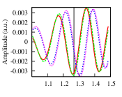
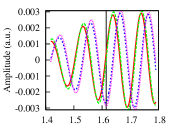
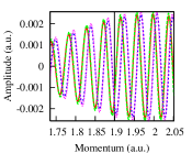
Figure 1: (Color online) Ionization from the $2s$ state of a Ne atom. ${\rm Re}f(k_{z},\Delta)$ computed using Eq. (8), solid (red) line, and TDSE calculation (green) dash. ${\rm Im}f(k_{z},\Delta)$ given by Eq. (8), (blue) short dash and TDSE (magenta) dots. XUV photon energies (top to bottom) are $\omega=68$, 81.6, and 95 eV. Delays $\Delta$ are (top to bottom) $0.2T$, $0.3T$, and $0.7T$, where $T$ is an optical cycle of the XUV pulse. Vertical solid line corresponds to the momentum $k_{z}$ for which $E_{0}+\omega=k_{z}^{2}/2$.

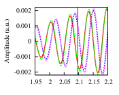
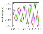
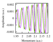
Figure 2: (Color online) Ionization from the $2s$ state of Ne atom. ${\rm Re}f(k_{z},\Delta)$ computed using Eq. (8), solid (red) line, and TDSE calculation (green) dash. ${\rm Im}f(k_{z},\Delta)$ given by Eq. (8), (blue) short dash and TDSE (magenta) dots. XUV photon energy $\omega=106$ eV. Delays $\Delta$ (top to bottom) are $\Delta=0.4T$, $\Delta=0.5T$, $\Delta=0.7T$, $T$ is an optical cycle of the XUV pulse. Vertical solid line corresponds to the momentum $k_{z}$ for which $E_{0}+\omega=k_{z}^{2}/2$.

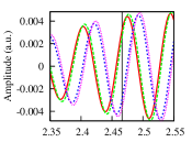
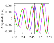
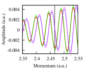
Figure 3: (Color online) Ionization from the $2p$ state of Ne atom. ${\rm Re}f(k_{z},\Delta)$ computed using Eq. (8), solid (red) line, and TDSE calculation (green) dash. ${\rm Im}f(k_{z},\Delta)$ given by Eq. (8), (blue) short dash and TDSE (magenta) dots. XUV photon energy $\omega=106$ eV. Delays $\Delta$ (top to bottom) are $\Delta=0.3T$, $\Delta=0.4T$, $\Delta=0.5T$, $T$ is an optical cycle of the XUV pulse. Vertical solid line corresponds to the momentum $k_{z}$ for which $E_{0}+\omega=k_{z}^{2}/2$.

The data displayed in these figures show that Eq. (8) allows to compute values of the two-color ionization amplitude $f(k_{z},\Delta)$ with a reasonable accuracy for ionization from $2s$ and $2p$ states of Ne provided we know the reference amplitude $f^{\rm XUV}(k_{z},0)$ as a function of the momentum. We may now try to solve an inverse problem of the reconstruction of the amplitude $f^{\rm XUV}(k_{z},0)$ provided that absolute values of the two-color amplitudes $f(k_{z},\Delta)$ are known for some selected values of the delays $\Delta$ and momenta $k_{z}$. This can be demonstrated as follows. We choose a trial form for the amplitude $f^{\rm XUV}(k_{z},0)$:

$$f^{\rm XUV}(k_{z},0)=Ae^{-a(E-\epsilon)^{2}+i\tau(E-\epsilon)},$$ (10)

where $E=k_{z}^{2}/2$, $a$, $\tau$, and $\epsilon$ are fitting parameters , and $A$ is a complex number which does not depend on the energy $E$. Parameter $\epsilon$ has a meaning of the energy at which the cross-section of the photo-ionization by the XUV pulse is peaked. The first guess for the value of this parameter can be obtained from the energy conservation $E_{0}+\omega=\epsilon_{0}$. We could fix the value of this parameter to $\epsilon_{0}$. However, more accurate results are obtained if we treat it as a fitting parameter. The parameter $\tau$, as can be immediately seen from the Eq. (9), has a meaning of the time delay.

The ansatz (10) does, in fact, a very good job at reproducing the amplitude $f^{\rm XUV}(k_{z},0)$ as Fig. 4 testifies. This figure shows comparison of a fit using the functional form (10) to the ’exact’ amplitude $f^{\rm XUV}(k_{z},0)$ which we obtain from the TDSE solution for ionization of the $2p$ sub-shell of the Ne atom by the XUV pulse.

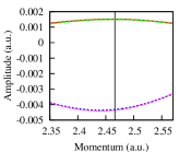
Figure 4: (Color online) ${\rm Re}f^{\rm XUV}(k_{z},0)$ computed using Eq. (10), solid (red) line, and TDSE calculation (green) dash. ${\rm Im}f^{\rm XUV}(k_{z},0)$ given by Eq. (10), (blue) short dash and TDSE (magenta) dots. XUV photon energy $\omega=106$ eV, ionization from the $2p$ state of Ne. Vertical solid line corresponds to the momentum $k_{z}$ for which $E_{0}+\omega=k_{z}^{2}/2$.

By using Eqs. (10) and (8), we can compute the trial amplitude $f^{t}(k_{z},\Delta)$ and, consequently, the trial electron spectrum $P^{t}(k_{z},\Delta)$ of the two-colour ionization of the Ne atom as a function of the momentum for various values of the delay $\Delta$ between the IR and XUV pulses. Using this distribution we can compute the trial expectation values of the electron momentum $\bar{k}^{t}_{z}(\Delta)$ for various $\Delta$:

$$\bar{k}^{t}_{z}(\Delta)=\int P^{t}(k_{z},\Delta)k_{z}\ dk_{z}\ ,$$ (11)

and compare them with the values $\bar{k}_{z}(\Delta)$ which we obtain from the TDSE calculation (and which can be measured in the experiment).

We can now form a functional:

$$D(a,\tau,\epsilon)=\sum\limits_{i}\left(\bar{k}^{t}_{z}(\Delta_{i})-\bar{k}_{z}(\Delta_{i})\right)^{2}$$ (12)

Sum in Eq. (12) is taken over a set of delays $\Delta$ between the IR and XUV pulses, for which the data are available. Presently, we use the set $\Delta=0.2T_{1}$, $0.3T_{1}$, $0.4T_{1}$, $0.5T_{1}$, and $0.7T_{1}$. By minimizing the functional (12) with respect to the parameters $a$, $\tau$, and $\epsilon$ in Eq. (10), we obtain the time-delay $\tau$.

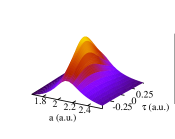
Figure 5: (Color online) Quantity $D^{-1}(a,\tau,\epsilon_{0})$ as function of $a$, and $\tau$. Value of $\epsilon_{0}$ is fixed at the energy conservation value $\epsilon_{0}=E_{0}+\omega$.

Convergence of this procedure is illustrated in Fig. 5 displaying the function $D^{-1}(a,\tau,\epsilon_{0})$ for fixed value of $\epsilon=\epsilon_{0}$, where $\epsilon_{0}=E_{0}+\omega$ is the value given by the energy conservation. This figure shows that $D^{-1}(a,\tau,\epsilon_{0})$ has a well-defined pronounced maximum in the space of the parameters $a,\tau$. This property is very useful since it implies that $D^{-1}(a,\tau,\epsilon)$ in Eq. (12) has a deep minimum, which is easy to locate.

Results of the procedure based on the minimization of the functional (12) are illustrated in Fig. 6, where we present the data for the time delay for several base frequencies $\omega$ of the XUV pulse for ionization from the $2s$ and $2p$ sub-shells of the Ne atom. These results are compared with the values for the time delays which we can extract directly from the TDSE calculation using the computed amplitudes of XUV photo-ionization and Eq. (9).

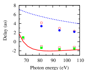
Figure 6: (Color online) Time delays computed using Eq. (9) and the fitting procedure. Ionization from the $2s$ state: (red) empty box- Eq. (9), (green) solid box- the fitting procedure. Ionization from the $2p$ state: (magenta) empty circle- Eq. (9), (blue) solid circle- the fitting procedure. The HF results: $2s\to Ep$ transition - (red) solid line, $2p\to Ed$ transition - (blue) dashed line.

Fig. 6 indicates that the results of the fitting procedure described above agree well with the results of the ab initio TDSE calculation. For completeness, in the same figure we display the time delay results obtained from the Hartree-Fock elastic scattering phases $\tau^{\rm HF}=d\delta^{\rm HF}_{l}/dE$. These phases are calculated in the frozen core Hartree-Fock approximation to electron scattering in the field of the Ne⁺ ion Kheifets (2013). The scattering phase in the dominant photoionization channel $l=l_{i}+1$ is taken according to the Fano propensity rule Fano (1985), where $l_{i}$ is the angular momentum of the initial bound state. Although these results are not directly comparable to the present calculations, which employ a localized effective potential, they demonstrate a qualitatively similar dependence of the time delay on the photon energy.

We may note that the present method of extraction of the attosecond time delay, based on the soft photon approximation, can be linked to the approach developed in Nagele et al. (2011); Pazourek et al. (2012); Nagele et al. (2012), which is a refinement of the strong field approximation Eq. (1). This refinement consists in introducing the correction factor, multiplying the vector potential in Eq. (1), and adding the so-called Coulomb-laser coupling correction in the argument of the function ${\bm{A}}^{\rm IR}(t)$. It is easy to see from Eqs. (8) and (10) that the photoelectron spectrum of the two-colour ionization $P(k_{z},\Delta)$ in the soft photon approximation can be represented as $P(k_{z},\Delta)=h(k_{z},\Delta+\tau)$, where $\tau$ is the time delay, and $h$ is a periodic function of the second argument with the period $T_{1}$ equal to the optical cycle of the IR field. The first moment of $P(k_{z},\Delta)$ can, therefore, be represented as $\bar{k}_{z}(\Delta)=q(\Delta+\tau)$, where $q$ is periodic with period $T_{1}$. We can write, therefore:

$$\bar{k}_{z}(\Delta)=\sum\limits_{n=0}^{\infty}B_{n}\sin{\Omega(\Delta+\tau)}+C_{n}\cos{\Omega(\Delta+\tau)}$$ (13)

The vector potential of the IR field described by Eq. (2) is $\displaystyle A^{\rm IR}(t)={{\cal E}_{0}^{\rm IR}\over\Omega}(1-\cos{\Omega t})\ .$ By retaining the terms with $n=0,1$ in Eq. (13) we obtain:

$$\bar{k}_{z}(\Delta)-b\approx cA^{\rm IR}(\Delta+\tau+\delta),$$ (14)

where the coefficients $b$, $c$, and $\delta$ can be expressed in terms of the coefficients of the Fourier expansion (13). By identifying the coefficients $b$, $c$ and $\delta$ in th Eq. (14) with $k_{z}^{0}$, the correction factor multiplying the vector potential in Eq. (1), and the Coulomb-laser coupling correction, we obtain the equation replacing the strong field relation (1) in the approach developed in Nagele et al. (2011); Pazourek et al. (2012); Nagele et al. (2012).

IV Conclusion

In the present work, we examined applicability of the soft photon approximation for evaluation of the amplitudes of two-colour XUV and IR ionization. We used the neon atom with a model localized potential as a convenient and representative numerical example. We have found that the two-colour ionization amplitudes, computed using the soft photon approximation, agree well with the ab initio TDSE amplitudes. This fact can be used to extract phase information and, in particular, the time delay from the experimental photoelectron spectra detected in attosecond streaking measurements. We tested the range of validity of the soft photon approximation. We demonstrated that this approximation renders the two-colour ionization amplitudes accurately for the IR field intensities in the range from $3.5\times 10^{10}$ to $5.6\times 10^{11}$ W/cm². The softness of the IR photon requires that its frequency should be much less than the kinetic energy of the photoelectron $\Omega/E_{\rm kin}\ll 1$. This means that the XUV photon energy should be well above the photoionization threshold. This is usually the case in the attosecond time delay measurements to minimize the effect of a large spectral width due to a short XUV pulse. It was found in Ref. Maquet and Taïeb (2007) that the soft photon approximation reproduces quite accurately the angle integrated cross sections for the values of this ratio as large as 0.06. We observed in the present study that the amplitudes were rendered accurately by the soft photon approximation for $\Omega/E_{\rm kin}\approx 0.07$ for the ionization from the inner $2s$ sub-shell of the Ne atom with the XUV frequency of 2.5 a.u. This defines the lower bound for the XUV frequency where we can use this approximation safely.

In our numerical examples, we confined ourselves to short XUV and IR pulses which are used in typical attosecond streaking experiments. However, in deriving our basic Eq. (8), we did not make any assumptions about the pulses duration. We can expect, therefore, that the applicability of the soft photon approximation to the two colour ionization process can be extended to longer IR pulses which lead to appearance of side bands in the photoelectron spectrum. It can be used, therefore, for the timing analysis of the photoelectron spectra obtained in RABITT experiments.

V Acknowledgment

The authors acknowledge support of the Australian Research Council in the form of Discovery grant DP120101805. Facilities of the National Computational Infrastructure National Facility were used.

References

- Wigner (1955) E. P. Wigner, Phys. Rev. 98, 145 (1955).
- de Carvalho and Nussenzveig (2002) C. A. A. de Carvalho and H. M. Nussenzveig, Phys. Rep. 364, 83 (2002).
- Schultze et al. (2010) M. Schultze, M. Fieß, N. Karpowicz, J. Gagnon, M. Korbman, M. Hofstetter, S. Neppl, A. L. Cavalieri, Y. Komninos, T. Mercouris, et al., Science 328, 1658 (2010).
- Eckle et al. (2008) P. Eckle, A. N. Pfeiffer, C. Cirelli, A. Staudte, R. Dörner, H. G. Muller, M. Büttiker, and U. Keller, Science 322, 1525 (2008).
- Paul et al. (2001) P. M. Paul, E. S. Toma, P. Breger, G. Mullot, F. Augé, P. Balcou, H. G. Muller, and P. Agostini, Science 202, 1689 (2001).
- Dahlström et al. (2012a) J. M. Dahlström, A. L’Huillier, and A. Maquet, J. Phys. B 45, 183001 (2012a).
- Dahlström et al. (2012b) J. M. Dahlström, T. Carette, and E. Lindroth, Phys. Rev. A 86, 061402(R) (2012b).
- Dahlström et al. (2013) J. M. Dahlström, D. Guénot, K. Klünder, M. Gisselbrecht, J. Mauritsson, A. L’Huillier, A. Maquet, and R. Taïeb, J. Chem. Phys. 414, 53 (2013).
- Itatani et al. (2002) J. Itatani, F. Quéré, G. L. Yudin, M. Y. Ivanov, F. Krausz, and P. B. Corkum, Phys. Rev. Lett. 88, 173903 (2002).
- Nagele et al. (2011) S. Nagele, R. Pazourek, J. Feist, K. Doblhoff-Dier, C. Lemell, K. Takasi, and J. Burgdörfer, J. Phys. B 44, 081001 (2011).
- Pazourek et al. (2012) R. Pazourek, J. Feist, S. Nagele, and J. Burgdörfer, Phys. Rev. Lett. 108, 163001 (2012).
- Nagele et al. (2012) S. Nagele, R. Pazourek, J. Feist, and J. Burgdörfer, Phys. Rev. A 85, 033401 (2012).
- Kroll and Watson (1973) N. M. Kroll and K. M. Watson, Phys. Rev. 8, 804 (1973).
- Maquet and Taïeb (2007) A. Maquet and R. Taïeb, J. Mod. Opt. 54, 1847 (2007).
- Sarsa et al. (2004) A. Sarsa, F. J. Gálvez, and E. Buendia, At. Data Nucl. Data Tables 88, 163 (2004).
- Duchateau et al. (2002) G. Duchateau, E. Cormier, and R. Gayet, Phys. Rev. A 66, 023412 (2002).
- Kornev and Zon (2002) A. S. Kornev and B. A. Zon, Journal of Physics B: Atomic, Molecular and Optical Physics 35, 2451 (2002).
- Ivanov and Kheifets (2013) I. A. Ivanov and A. S. Kheifets, Phys. Rev. A 87, 033407 (2013).
- Ivanov (2011) I. A. Ivanov, Phys. Rev. A 83, 023421 (2011).
- Kheifets (2013) A. S. Kheifets, ArXiv e-prints p. 1302.4495 (2013), URL http://arxiv.org/abs/1302.4495.
- Fano (1985) U. Fano, Phys. Rev. A 32, 617 (1985).