Examples of infinitesimal non-trivial accumulation of secants in dimension three

Abstract

We present new examples of accumulation of secants for orbits (of a real analytic three dimensional vector fields) having the origin as only $\omega$-limit point. These new examples have the structure of a proper algebraic variety of $\mathbb{S}^{2}$ intersected with a cone. In particular, we present explicit examples of accumulation of secants sets which are not in the list of possibilities of the classical Poincaré-Bendixson Theorem.

Keywords Accumulation of secants, Ordinary Differential Equations, Real analytic geometry.

Contents

1. 1 Introduction
2. 2 The $\Gamma$-convergence
3. 3 Construction in a chart
4. 4 Globalization
5. 5 Isolated singularity

1 Introduction

Let $X$ be a real analytic vector-field defined in a neighborhood of the origin of $\mathbb{R}^{3}$ and assume that the origin is a singularity of $X$. Consider a regular orbit $\gamma(t)$ of $X$ such that the origin is the only $\omega$-limit point of $\gamma(t)$, i.e $lim_{t\rightarrow\infty}\gamma(t)=(0,0,0)$. A classical problem is to study the qualitative behavior of the trajectory $\gamma(t)$ (see, for example, [Le, Ly, P]). A modern approach to this problem is to ask for a description of the accumulation of secants of $\gamma(t)$.

More precisely, let the curve $\frac{\gamma(t)}{\|\gamma(t)\|}\subset\mathbb{S}^{2}$ be the secants curve of $\gamma(t)$. The accumulation of secants is the set:

$$Sec(\gamma(t))=\bigcap_{s}\overline{\{\gamma(t)/\|\gamma(t)\|;t\geq s\}}\subset\mathbb{S}^{2}$$

In the literature we can find descriptions of accumulation os secants for some classes of three dimensional vector-fields. For example:

• In [GCaR] the authors provide a description of the accumulation of secants $Sec(\gamma(t))$ under the hypotheses that the origin is a generic absolutely isolated singularity (see definition in the same article);

• In [CaMoS1, CaMoR, CaMoS2, CaMoS3], the authors study properties of orbits under some additional oscillating hypotheses (as, the so-called, sub-analytically non-oscillating property).

But, the problem of giving a description of the accumulation on secants $Sec(\gamma(t))$ for general three dimensional vector-fields is widely open. In one hand, it is still an open question whether there exists an accumulation of secants set $Sec(\gamma(t))$ which is dense on the sphere. At another hand, all examples in the literature are contained in the list of possibilities given by the Poincaré-Bendixson Theorem.

In this work, we prove that a connected component of a proper algebraic variety of $\mathbb{S}^{2}$ intersected with a cone may be realized as an accumulation of secants set. In particular, we present a wide class of examples of accumulations of secants sets which are not in the list of possibilities of the Poincaré-Bendixson Theorem (see figure (1) for an example). Furthermore, the vector-fields that give rise to these new examples are explicit and polynomial.

In order to be precise, consider a non-zero real-polynomial $h\in\mathbb{R}[x,y]$ and let $\Gamma$ be the semi-algebraic set $V(h)\cap B_{1}(0)$, where $B_{1}(0)$ is the closed ball with radius one and center at the origin and $V(h)=\{p\in\mathbb{R}^{2};h(p)=0\}$ is the algebraic variety given by the zeros of the polynomial $h$. We say that the polynomial $h$ is adapted if:

• The set $\Gamma$ is connected and non-empty;

• The algebraic variety $V(h,\frac{\partial}{\partial x}h,\frac{\partial}{\partial y}h)=V(h,h_{x},h_{y})$ is equal to a finite set of points;

• The set $V(h)\cap\partial B_{1}(0)$ is a finite set of points such that $<\nabla^{\bot}h(p),p>\neq 0$, where $\partial B_{1}(0)$ stands for the border of $B_{1}(0)$.

Now, consider the following chart of $\mathbb{S}^{2}$:

$$\begin{array}[]{cccl}\alpha:&\mathbb{R}^{2}&\longrightarrow&\mathbb{S}^{2}\\ &(x,y)&\mapsto&\left(\frac{x}{\sqrt{x^{2}+y^{2}+1}},\frac{y}{\sqrt{x^{2}+y^{2}+1}},\frac{1}{\sqrt{x^{2}+y^{2}+1}}\right)\end{array}$$

With this notation, the main result of this work can be precisely enunciated:

Theorem 1.1.

Let $h\in\mathbb{R}[x,y]$ be an adapted polynomial. There exists a real three dimensional polynomial vector-field $X$ and a regular orbit $\gamma(t)$ of $X$ such that:

• ) The $\omega$-limit of the orbit $\gamma(t)$ is an isolated singularity of $X$;

• ) The accumulation of secants set $Sec(\gamma(t))$ is equal to $\alpha(\Gamma)$.

Example 1: A first non-trivial example can be given by the simple function:

$$h(x,y)=(x^{2}-\frac{1}{4})(y^{3}-\frac{1}{4}y)$$

Notice that the set $\Gamma=V(h)\cap B_{1}(0)$ is not in the list of possibilities given by the Poincaré-Bendixson Theorem (see figure 1). Moreover, since $h$ is adapted, Theorem 1.1 guarantees that $\alpha(\Gamma)$ is an accumulation of secants for some algebraic vector-field $X$.

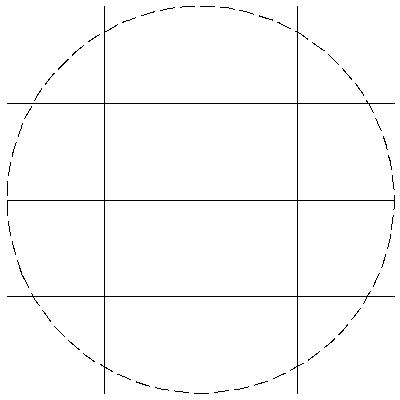
Figure 1: The set $\Gamma=V(h)\cap B_{1}(0)$ of example 1.

The proof of Theorem 1.1 is a direct consequence of Theorem 5.1 and Proposition 5.2 below. Nevertheless, it is worth remarking that Propositions 2.3 and 4.1 below are enough to prove property $[ii]$ of the Theorem.

To conclude, we would like to remark that the ideas behind this work may lead to a stronger result. We believe that it should be possible to prove that any proper and connected semi-algebraic variety of $\mathbb{S}^{2}$ (maybe satisfying some generic condition) may be realized as an accumulation of secants set for some algebraic vector-field $X$.

Remark 1.2.

In the rest of the manuscript we study the convergence of the orbit $\gamma(t)$ after the projective blowing-up of the origin:

$$\tau:\mathbb{R}\times\mathbb{P}^{2}\longrightarrow\mathbb{R}^{3}$$

instead of the secants of $\gamma(t)$. We remark that this treatment leads to the desired result because $\mathbb{S}^{2}$ is a double cover of $\mathbb{P}^{2}$.

2 The $\Gamma$-convergence

Consider a real polynomial $H\in\mathbb{R}[x,y,z]$ and a compact and connected sub-set $\Gamma$ of $\mathbb{R}^{2}$. Let $L_{z_{0}}$ be the variety $V(H,z-z_{0})$ for any constant $z_{0}$ in $\mathbb{R}$. We say that the polynomial $H$ is $\Gamma$-convergent if the varieties $L_{z_{0}}$, with positive constants $z_{0}$, converge (in the Hausdorff topology) to $\Gamma$ when $z_{0}$ converges to zero, i.e. $L_{z_{0}}\stackrel{{\scriptstyle z_{0}\rightarrow 0^{+}}}{{\longrightarrow}}\Gamma\times\{0\}$.

Remark 2.1.

The fact that a polynomial $H$ is $\Gamma$-convergent does not imply that the variety $L_{0}$ is equal to $\Gamma$.

Furthermore, we say that $H$ is:

• connected $\Gamma$-convergent if there exists a positive real number $\epsilon$ such that $L_{z}$ is a connected variety for $0<z<\epsilon$;

• smooth $\Gamma$-convergent if there exists a positive real number $\epsilon$ such that $L_{z}$ is a smooth variety for $0<z<\epsilon$.

Remark 2.2.

If $H$ is connected $\Gamma$-convergent then, for a small enough positive real number $\epsilon$, the semi-analytic variety $V(H)\cap\{0<z<\epsilon\}$ is homeomorphic to a topological cylinder.

If $\Gamma$ is equal to a semi-analytic variety $V(h)\cap\{x^{2}+y^{2}\leq 1\}$, where $h$ is an adapted polynomial (see definition in the introduction), then Propositions $[2.1-2.2]$ of [Be] guarantees the existence of a polynomial $H$ that is smooth connected $\Gamma$-convergent. More precisely, in [Be] it is consider the family of polynomials:

$$H_{\alpha}(x,y,z)=h(x,y)^{2}+g(x,y,z)+\alpha z^{4}$$

where the parameter $\alpha$ takes values in the interval $[0,1]$ and the polynomial $g(x,y,z)$ has the form $z(\widetilde{g}(x,y,z)+\sum^{N}_{i=1}\binom{N}{i}x^{2i}y^{2(N-i)})$ for some $N\in\mathbb{N}$, where $\widetilde{g}(x,y,z)$ is a polynomial with degree strictly smaller than $2N$. We remark that the explicit expression of the polynomial $g(x,y,z)$ can be found in [Be], but is not important for this work. Finally, Propositions $[2.1-2.2]$ of [Be] are sufficient to prove the following:

Proposition 2.3.

If $\Gamma$ is equal to a semi-analytic variety $V(h)\cap\{x^{2}+y^{2}\leq 1\}$, where $h$ is an adapted polynomial, then there exists a polynomial $H$ smooth connected $\Gamma$-convergent. Furthermore, such a polynomial can be chosen as the polynomials $H_{\alpha}(x,y,z)$ for almost all $\alpha$ fixed.

In what follows we work with any polynomial $H(x,y,z)$ that is smooth connected $\Gamma$-convergent.

3 Construction in a chart

We say that a real three dimension vector-field $X$ is $\Gamma$-convergent if the variety $\{z=0\}$ is invariant by $X$, i.e. $X$ is tangent to $\{z=0\}$, and there exists an orbit $\gamma(t)$ of $X$ contained in $\{z>0\}$ such that the $\omega$-limit of $\gamma(t)$ is equal to $\Gamma\times\{0\}$.

In this section, we prove that the existence of a polynomial smooth connected $\Gamma$-convergent implies the existence of a vector-field $\Gamma$-convergent. More precisely, let $H$ be smooth connected $\Gamma$-convergent and consider:

• The $H$-horizontal vector-field $\mathcal{H}(H)=-H_{y}\frac{\partial}{\partial x}+H_{x}\frac{\partial}{\partial y}$;

• The $H$-vertical vector-field $\mathcal{V}(H)=\mathcal{V}(H):=H_{x}H_{z}\frac{\partial}{\partial x}+H_{y}H_{z}\frac{\partial}{\partial y}-(H_{x}^{2}+H^{2}_{y})\frac{\partial}{\partial z}$;

• The $H$-perturbed vector-field $\mathcal{P}(H):=H\frac{\partial}{\partial z}$.

Notice that, for a small enough $\epsilon>0$:

• The $H$-horizontal vector-field $\mathcal{H}(H)$ is the Hamiltonian of the function $H$ in respect to the variables $(x,y)$;

• The $H$-horizontal vector-field $\mathcal{H}(H)$ and the $H$-vertical vector-field $\mathcal{V}(H)$ forms a base of $T_{p}V(H)$ for all points $p$ in the intersection of $V(H)$ and $\{0<z<\epsilon\}$.

• The $H$-perturbed vector-field $\mathcal{P}(H)$ is identically zero in $V(H)$.

Now, consider the polynomial family of vector-fields:

$$X_{\beta_{1},\beta_{2}}(H)=\mathcal{H}(H)+z^{\beta_{1}}\mathcal{V}(H)+z^{\beta_{2}}\mathcal{P}(H)$$

for constants $\beta_{1}$ and $\beta_{2}$ in $\mathbb{N}\setminus\{0\}$. The main result of this section can now be formulated precisely:

Proposition 3.1.

Suppose that there exists a polynomial $H$ smooth connected $\Gamma$-convergent. Then, for any big enough $\beta_{1}$ and any positive $\beta_{2}$, the vector-field $X_{\beta_{1},\beta_{2}}(H)$ constructed above is $\Gamma$-convergent.

Proof.

Fix a constant $\beta_{2}>0$ and let $X_{\beta_{1}}$ denote the vector-field $X_{\beta_{1},\beta_{2}}(H)$ with the fixed $\beta_{2}$. By construction, it is clear that the vector-field $X_{\beta_{1}}$ is tangent to the variety $V(H)$ and to the plane $\{z=0\}$, which implies that the semi-algebraic set $V(H)\cap\{z\geq 0\}$ is invariant by the flux of $X_{\beta_{1}}$.

We claim that for $\beta_{1}$ big enough, there exists $\epsilon>0$ such that all orbits of $X_{\beta_{1}}$ passing by $V(H)\cap\{0<z<\epsilon\}$ have $\omega$-limit equal to $\Gamma\times\{0\}$. Indeed, consider $\epsilon>0$ sufficiently small, so that we can define the analytic diffeomorphism:

$$\pi:\mathbb{S}^{1}\times\{0<r<\epsilon\}\to V(H)\cap\{0<z<\epsilon\}$$

where $\pi(\theta,r)=(x(\theta,r),y(\theta,r),r)$. We remark that one can prove the existence of such a map using the flux of the horizontal vector-field $\mathcal{H}(H)$.

Remark 3.2 (This remark is supposed to be removed).

. Since the horizontal vector-field $Y=\mathcal{H}(H)$ is analytic (even algebraic), the regular orbits of this vector-field are analytic functions and the dependence of the initial condition is also analytic. So, let $\Sigma$ be an analytic transverse section of $Y$ which is contained in $V(H)\cap\{0<z<\epsilon\}$. Then the return map is well-defined and the function $T:\Sigma\to\mathbf{R}$ which gives the time of return is an analytic function which is always positive. We will use the analytic vector field $\frac{Y}{T}$, where we abuse notation to define $T$ over all $V(H)\cap\{0<z<\epsilon\}$ by letting it be constant over the orbits of $Y$. So, we can consider the orbits $\phi:\mathcal{R}\times\Sigma\to V(H)\cap\{0<z<\epsilon\}$ where $\phi(t,p)$ is the orbit of the vector-field $\frac{Y}{T}$ with initial condition $p$ and time $t$. Since $\Sigma$ is clearly biholomorphic with $(0,\epsilon)$, this gives rise to the necessary analytic map.

Furthermore, I believe the map can not be algebraic because we are using polar coordinates.

We work with the pull-back of $X_{\beta_{1}}$ under this map:

$$\pi^{\ast}\mathcal{H}(H) =A(\theta,r)\frac{\partial}{\partial\theta}$$

$$\pi^{\ast}\mathcal{V}(H) =B(\theta,r)\frac{\partial}{\partial\theta}-C(\theta,r)\frac{\partial}{\partial r}$$

$$\pi^{\ast}X_{\beta_{1}} =[A(\theta,r)+r^{\beta_{1}}B(\theta,r)]\frac{\partial}{\partial\theta}-r^{\beta_{1}}C(\theta,r)\frac{\partial}{\partial r}$$

where the functions $A$, $B$ and $C$ are analytic functions over the cylinder $\mathbb{S}^{1}\times\{0<r<\epsilon\}$.

Now, we claim that the function $A$ and $C$ are strictly positive functions. Indeed, apart from taking a smaller $\epsilon$, we notice that the vector-field $\mathcal{H}(H)$ has no singularities since $H$ is $\Gamma$-convergent (thus, the intersection of the variety $V(H,H_{x},H_{y})$ with the set $\{0<z<\epsilon\}$ is empty). This implies that $A$ is of a fixed sign for $r>0$ and, apart from changing the sign of $\theta$, we can assume that it is positive.

Furthermore, notice that the function $L:=z$ is a strict negative Lyapunov function of $\mathcal{V}(H)$ over the semi-analytic set $V(H)\cap\{0<z<\epsilon\}$. Indeed, for a point $p$ in $V(H)\cap\{0<z<\epsilon\}$:

$$[\mathcal{V}(H)](L)=[-z^{\beta_{1}}(H_{x}^{2}+H^{2}_{y})]<0$$

This implies that $-C=\pi*[\mathcal{V}(H)](L)<0$ and $C$ is strictly positive function. We remark that this already implies that all orbits of $X_{\beta_{1}}$ passing by $V(H)\cap\{0<z<\epsilon\}$ have $\omega$-limit contained in $\Gamma\times\{0\}$

To be able to conclude, we just need to show that $\frac{rd\theta}{dr}>1$ for all $\theta$ in $\mathbb{S}^{1}$ and all $r$ sufficiently small. This would clearly imply that the vector-field $\pi^{\ast}X_{\beta_{1}}$ is spiraling, i.e its orbits have the hole $\mathbb{S}^{1}\times\{0\}$ as a $\omega$-limit. Finally, this would imply that all orbits of $X_{\beta_{1}}$ passing by $V(H)\cap\{0<z<\epsilon\}$ have $\omega$-limit equal to $\Gamma\times\{0\}$.

So, we just have to prove that the following inequality holds:

$$\frac{A}{Cr^{\beta_{1}-1}}+\frac{rB}{C}>1$$ (1)

To be able to do so, we use Lojasiewicz’s inequality for semi-analytic sets (see Theorem 6.4 of [BiMi]). We actually use a slightly stronger result which can be easily deduced from the proof given in Theorem 6.4 of [BiMi] (for the excat same remark for quasi-algebraic category, see Proposition $2.11$ of [Co] and remark (a) below the same Proposition):

Proposition 3.3.

Let $K$ be a semi-nalytic set of $\mathbb{R}^{n}$, $f$ and $g$ two continuous and semi-analytic functions over $K$ such that:

• ) The set $\{x\in K;\|g(x)\|>\delta\}$ is compact for all $\delta>0$;

• ) The zeros of $f$ are also zeros of $g$.

Then, there exists strictly positive constants $M$ and $\alpha$ such that $\|f(x)\|\geq M\|g(x)\|^{\alpha}$ for all $x$ in $K$.

The idea is to apply this result for the semi-algebraic set $K=\mathbb{S}^{1}\times\{0<r<\epsilon\}$ and for the function $g=r$. We notice that these choices of $K$ and $g$ clearly satisfies hypothesis $[i]$ of Proposition 3.3. So, we can directly apply Proposition 3.3 to the functions $A$, $C$ and $\frac{1}{C}$ in order to obtain positive constants $M$, $a$, $c_{1}$ and $c_{2}$ such that: $A>Mr^{a}$; $C>Mr^{c_{1}}$ and $\frac{1}{C}>Mr^{c_{2}}$.

We notice that one can not apply Proposition 3.3 directly to $B$ since the function $B$ may have zeros on $K$. Nevertheless, since $B$ is analytic on $K$, let us consider the two semi-algebraic sets $K_{1}=K\cap\{B>-1\}$ and $K_{2}=K\cap\{B\leq-1\}$, where $K_{2}$ is relatively compact. In this situation, we can apply Proposition 3.3 to the function $\frac{1}{B}$ over $K_{2}$ in order to obtain a positive constant $b$ such that, without loss of generality: $-\frac{1}{B}>Mr^{b}$, which implies that $B>-Mr^{-b}$.

So, for a point $p$ in $K_{1}$, we obtain:

$$\frac{A}{Cr^{\beta_{1}-1}}+\frac{rB}{C}>Ar^{1-\beta_{1}}\frac{1}{C}-r\frac{1}{C}>Mr^{a}r^{1-\beta_{1}}Mr^{c_{2}}-rM^{-1}r^{-c_{1}}=$$

$$=M^{2}r^{1+a+c_{2}-\beta_{1}}-M^{-1}r^{1-c_{1}}$$

and for $p$ in $K_{2}$, we obtain:

$$\frac{A}{Cr^{\beta_{1}-1}}+\frac{rB}{C}>Ar^{1-\beta_{1}}\frac{1}{C}-Mr^{-b}\frac{1}{C}>Mr^{a}r^{1-\beta_{1}}Mr^{c_{2}}-Mr^{-b}M^{-1}r^{-c_{1}}=$$

$$=M^{2}r^{1+a+c_{2}-\beta_{1}}-r^{1-c_{1}-b}$$

So, it is clear that for $r$ sufficiently small and $\beta_{1}$ sufficiently big, the inequality $(\ref{eq:2})$ is satisfied for all points in $K=K_{1}\cup K_{2}$, as we wanted to prove. ∎

4 Globalization

In this section, we prove that the existence of a polynomial $H$ smooth connected $\Gamma$-convergent implies the existence of a vector-field with an orbit $\gamma(t)$ such that its accumulation of secants set $Sec(\gamma(t))$ is $\alpha(\Gamma)$ (see the definition of the morphism $\alpha:\mathbb{R}^{2}\longrightarrow\mathbb{S}^{2}$ in the introduction). More precisely, let $H$ be a smooth connected $\Gamma$-convergent and consider the subset of polynomials:

$$\mathcal{O}^{{}^{\prime}}_{\mathbb{R}^{3}}=\{f\in\mathcal{O}_{\mathbb{R}^{3}};\text{ }f(0,0,0)=0\text{ and }f(x,y,0)\not\equiv 0\}$$

and the function:

$$\begin{array}[]{cccc}\sigma:&\mathbb{R}^{3}&\longrightarrow&\mathbb{R}^{3}\\ &(x,y,z)&\mapsto&(xz,yz,z)\end{array}$$

which is also equal to a blowing-up restricted to one of its charts. Then, there exists two unique functions:

$$\begin{array}[]{ccc}\phi:\mathcal{O}^{{}^{\prime}}_{\mathbb{R}^{3}}\longrightarrow\mathbb{N}^{\ast}&\text{ , }&\psi:\mathcal{O}_{\mathbb{R}^{3}}\longrightarrow\mathcal{O}^{{}^{\prime}}_{\mathbb{R}^{3}}\end{array}$$

such that:

$$z^{\phi(f)}f=\psi(f)\circ\sigma$$

Now, fix constants:

• $\alpha=max\{\phi(H_{y}),\phi(H_{x})\}$;

• $\beta_{1}\geq 2[\phi(H_{x})+\phi(H_{y})]+\phi(H_{z})-\alpha+2$ (in particular $\beta_{1}\geq 1$);

• $\beta_{2}=\phi(H)-\alpha+1$ (in particular $\beta_{2}\geq 1$).

Notice that $\beta_{1}$ can be chosen as big as necessary. We define the vector-field:

$$Y=A\frac{\partial}{\partial x}+B\frac{\partial}{\partial y}+C(x\frac{\partial}{\partial x}+y\frac{\partial}{\partial y}+z\frac{\partial}{\partial z})$$

where:

• $A=-z^{a_{1}}\psi(H_{y})+z^{a_{2}}\psi(H_{x})\psi(H_{z})$ where:

  $$\begin{array}[]{c}a_{1}=\alpha+1-\phi(H_{y})\geq 1\\ a_{2}=\alpha+\beta_{1}+1-\phi(H_{x})-\phi(H_{z})\geq 1\end{array}$$

• $B=z^{b_{1}}\psi(H_{x})+z^{b_{2}}\psi(H_{y})\psi(H_{z})$ where:

  $$\begin{array}[]{c}b_{1}=\alpha+1-\phi(H_{x})\geq 1\\ b_{2}=\alpha+\beta_{1}+1-\phi(H_{y})-\phi(H_{z})\geq 1\end{array}$$

• $C=-z^{c_{1}}\psi(H_{x})^{2}-z^{c_{2}}\psi(H_{y})^{2}+\psi(H)$ where:

  $$\begin{array}[]{c}c_{1}=\alpha+\beta_{1}-1-2\phi(H_{x})\geq 1\\ c_{2}=\alpha+\beta_{1}-1-2\phi(H_{y})\geq 1\end{array}$$

The main result of this section can now be formulated precisely:

Theorem 4.1.

Suppose that there exists a polynomial $H$ smooth connected $\Gamma$-convergent. Then, for $\beta_{1}$ sufficiently big, the vector-field $Y$ constructed above has a regular orbit $\gamma(t)$ such that the accumulation of secants $Sec(\gamma(t))$ is equal to $\alpha(\Gamma)$ (see the definition of the morphism $\alpha:\mathbb{R}^{2}\longrightarrow\mathbb{S}^{2}$ in the introduction).

Proof.

Consider the blowing-up of $\mathbb{R}^{3}$ with the origin as center:

$$\tau:\mathbb{R}\times\mathbb{P}^{2}\longrightarrow\mathbb{R}^{3}$$

and let $Y^{{}^{\prime}}$ be the strict transform of the vector-field $Y$. Then, in the $z$-chart, the strict transform $Y^{{}^{\prime}}$ is equal to $X_{\beta_{1},\beta_{2}}(H)$. Indeed:

$$Y^{{}^{\prime}}=z^{-\alpha}Y^{\ast}=z^{-(\alpha+1)}A^{\ast}\frac{\partial}{\partial x}+z^{-(\alpha+1)}B^{\ast}\frac{\partial}{\partial y}+z^{-\alpha}C^{\ast}(z\frac{\partial}{\partial z})$$

where:

• $z^{-(\alpha+1)}A^{\ast}=-z^{a^{\ast}_{1}}H_{y}+z^{a^{\ast}_{2}}H_{x}H_{z}$ where:

  $$\begin{array}[]{c}a^{\ast}_{1}=\alpha+1-\phi(H_{y})+\phi(H_{y})-\alpha-1=0\\ a^{\ast}_{2}=\alpha+\beta_{1}+1-\phi(H_{x})-\phi(H_{z})+\phi(H_{x})+\phi(H_{z})-\alpha-1=\beta_{1}\end{array}$$

• $z^{-(\alpha+1)}B^{\ast}=-z^{b^{\ast}_{1}}H_{y}+z^{b^{\ast}_{2}}H_{x}H_{z}$ where:

  $$\begin{array}[]{c}b^{\ast}_{1}=\alpha+1-\phi(H_{x})+\phi(H_{x})-\alpha-1=0\\ b^{\ast}_{2}=\alpha+\beta_{1}+1-\phi(H_{y})-\phi(H_{z})+\phi(H_{y})+\phi(H_{z})-\alpha-1=\beta_{1}\end{array}$$

• $z^{-\alpha}C^{\ast}=-z^{c^{\ast}_{1}}H_{x}^{2}-z^{c^{\ast}_{2}}H_{y}^{2}+z^{c^{\ast}_{3}}H$ where:

  $$\begin{array}[]{c}c^{\ast}_{1}=\alpha+\beta_{1}-1-2\phi(H_{x})+2\phi(H_{x})-\alpha=\beta_{1}-1\\ c^{\ast}_{2}=\alpha+\beta_{1}-1-2\phi(H_{y})+2\phi(H_{y})-\alpha=\beta_{1}-1\\ c^{\ast}_{3}=\phi(H)-\alpha=\beta_{2}-1\end{array}$$

Since, by Proposition 3.1, the vector-field $X_{\beta_{1},\beta_{2}}(H)$ is $\Gamma$-convergent for $\beta_{1}$ big enough, the thesis clearly follows. ∎

5 Isolated singularity

In this subsection, we prove that the vector-field $Y$ of Theorem 4.1 can be chosen so that the origin is an isolated singularity. For this end, we need to strengthen the hypotheses over the polynomial $H$ that is $\Gamma$-convergent.

We say that a polynomial $H$ is isolated $\Gamma$-convergent if:

• ) There exists a positive real number $\epsilon$ such that $L_{z}$ is a smooth variety for $-\epsilon<z<0$;

• ) The origin of $\mathbb{R}^{2}$ is an isolated solution of the equation in two variables $\{\psi(H)(x,y,0)=0\}$.

With this definition, we can prove the following result:

Theorem 5.1.

Suppose that there exists a polynomial $H$ isolated smooth connected $\Gamma$-convergent. Then, the origin is an isolated singularity of the vector-field $Y$ constructed in Theorem 4.1.

Proof.

Notice that the vector-field $Y$ constructed in Theorem 4.1 is such that:

$$Y(x,y,0)=C(x,y,0)(x\frac{\partial}{\partial x}+y\frac{\partial}{\partial y})$$

and, by construction:

$$C(x,y,0)=[-z^{c_{1}}\psi(H_{x})^{2}-z^{c_{2}}\psi(H_{y})^{2}+\psi(H)](x,y,0)=\psi(H)(x,y,0)$$

because the natural constants $c_{1}$ and $c_{2}$ are not $0$. Since $H$ is isolated $\Gamma$-convergent, we conclude that there exists a positive real number $\delta$ such that the intersection of the singularities of $Y$ intersected with the variety $V(z)$, with the ball of radius $\delta$ and center in the origin is just the origin, i.e.:

$$Sing(Y)\cap\{z=0\}\cap B_{\delta}(0)=\{(0,0,0)\}$$

Thus, we only need to search singularities of $Y$ outside the plane $V(z)$, which can be done in the $z$-chart of the blowing-up of the origin. By construction, after blowing-up the origin the vector-field $Y$ is transformed into the vector-field $X_{\beta_{1},\beta_{2}}(H)$. We now study the singularities of this vector-field:

Claim: The set of singularities $Sing(X_{\beta_{1},\beta_{2}})$ is equal to the variety $V(zH,H_{x},H_{y})$.

Proof.

By construction of the vector-field $X_{\beta_{1},\beta_{2}}(H)$, it is clear that $V(zH,H_{x},H_{y})\subset Sing(X_{\beta_{1},\beta_{2}})$. So consider a point $p$ in $Sing(X_{\beta_{1},\beta_{2}}(H))$. We have that:

$$\begin{array}[]{c}\left[H_{y}-z^{\beta_{1}}H_{z}H_{x}\right](p)=0\\ \left[H_{x}+z^{\beta_{1}}H_{z}H_{y}\right](p)=0\\ \left[-z^{\beta_{1}}(H^{2}_{x}+H^{2}_{y})+z^{\beta_{2}}H\right](p)=0\end{array}$$

From the first equation, we have that $H_{y}(p)=z^{\beta_{1}}H_{z}H_{x}(p)$. Replacing this expression in the second equation, we get that $[H_{x}(1+z^{2\beta_{1}}H^{2}_{z})](p)=0$, which implies that $H_{x}(p)=0$. Thus, $H_{y}(p)=0$. Replacing this in the last equation, we finally get that either $z(p)=0$ or $H(p)=0$. ∎

Notice that the hypotheses over the polynomial $H$ implies that the varieties $L_{z}$ are all smooth for $z$ small enough (positive or negative) different from zero. This clearly implies that the intersection of the variety $V(H,H_{x},H_{y})$ with the set $\{-\epsilon<z<\epsilon\}$ is all contained in $\{z=0\}$. Furthermore, by the Claim, taking a smaller $\delta>0$ if necessary, the singularities of the vector-field $X_{\beta_{1},\beta_{2}}(H)$ intersected with the set $\{-\epsilon<z<\epsilon\}$ is all contained in $\{z=0\}$ (which is the exceptional divisor). This finally implies that:

$$Sing(Y)\cap B_{\delta}(0)=\{(0,0,0)\}$$

and the origin is an isolated singularity. ∎

To finish the proof of Theorem 1.1, we need to prove the existence of polynomials $H$ isolated smooth connected $\Gamma$-convergent.

Proposition 5.2.

If $\Gamma$ is equal to a semi-analytic variety $V(h)\cap\{x^{2}+y^{2}\leq 1\}$, where $h$ is an adapted polynomial, then there exists a polynomial $H$ isolated smooth connected $\Gamma$-convergent.

Proof.

We recall that:

$$H_{\alpha}(x,y,z)=h(x,y)^{2}+g(x,y,z)+\alpha z^{4}$$

where the parameter $\alpha$ takes values in the interval $[0,1]$ and the polynomial $g(x,y,z)$ has the form $z(\widetilde{g}(x,y,z)+\sum^{N}_{i=1}\binom{N}{i}x^{2i}y^{2(N-i)})$ for some $N\in\mathbb{N}$, where $\widetilde{g}(x,y,z)$ is a polynomial with degree strictly smaller than $2N$.

In particular, notice that $(0,0)$ is an isolated solution of the equation $\psi(g)(x,y,0)=0$. So, if we can choose $g$ such that $\phi(g)\geq\phi(h^{2})$ and $\phi(g)>4$, we have that $(0,0)$ is an isolated solution of $\psi(H)(x,y,0)=0$.

But this property is not generally true for the polynomial $g(x,y,z)$ given in [Be]. So consider $f(x,y)=((x-x_{0})^{2}+(x-y_{0})^{2})^{M}$ where $(x_{0},y_{0})$ is a point outside the ball with radius one and the variety $V(h)$, i.e. $p\notin V(h)\cup B_{1}(0)$, and $M$ is a natural number sufficiently big. It is clear that:

• The polynomial $g(x,y,z)f(x,y)$ is equal to $z(\bar{g}(x,y,z)+\sum^{N+M}_{i=1}\binom{N+M}{i}x^{2i}y^{2(N-i)})$, where $\bar{g}(x,y,z)$ is a polynomial with degree strictly smaller than $2(N+M)$;

• For $M$ sufficiently big, we have that: $\phi(gf)\geq\phi(h^{2})$ and $\phi(gf)>4$.

So, we consider:

$$\widetilde{H}_{\alpha}(x,y,z)=h(x,y)^{2}+f(x,y)g(x,y,z)-\alpha z^{4}$$

It is now clear that property $[ii]$ of the definition of isolated $\Gamma$-convergent is satisfied. The proof that this polynomials (for almost all $\alpha$ in $[0,1]$) is isolated smooth connected $\Gamma$-convergent now follows, mutatis mutandis, the same proof of Propositions $[2.1-2.2]$ of [Be]. Nevertheless, we remark two crucial details for the necessary adaptations:

• Lemma $3.3$ of [Be] contains the proof of property $[i]$ of the definition of isolated $\Gamma$-convergent, although it does not enunciate it;

• The polynomial $f(x,y)$ is a positive unity over any small enough neighborhood of $B_{1}(0)$.

∎

References

• [Be] Belotto, A. Analytic varieties as limit periodic sets, Qualitative Theory of Dynamical Systems October 2012, Volume 11, Issue 2, pp 449-465.
• [BiMi] Bierstone, Edward; Milman, Pierre D. Semianalytic and subanalytic sets. Inst. Hautes Γ‰tudes Sci. Publ. Math. No. 67 (1988), 5?42.
• [CaMoR] F. Cano, R. Moussu, and J. P. Rolin, Non-oscillating integral curves and valuations. J. Reine Angew. Math. 582 (2005), 107-141.
• [CaMoS1] Cano, F.; Moussu, R.; Sanz, F. Nonoscillating projections for trajectories of vector fields. J. Dyn. Control Syst. 13 (2007), no. 2, 173-176.
• [CaMoS2] F. Cano, R. Moussu, and F. Sanz, Oscillation, spiralement, tourbillonnement. Comment. Math. Helv. 75 (2000), 284-318.
• [CaMoS3] F. Cano, R. Moussu, and F. Sanz, Pinceaux de courbes intΓ©grales d’un champ de vecteurs analytique. AstΓ©risque 297 (2004), 1-34.
• [Co] Coste, Michel, Ensembles semi-algebriques, GΓ©omΓ©trie AlgΓ©brique RΓ©elle et Formes Quadratiques, Ed: Colliot-ThΓ©lΓ¨ne, J; E. Coste; M., E MahΓ©; L.; E Roy, M-F; Springer Berlin Heidelberg, 1982, 109-138.
• [GCaR] C. Alonso-GonzΓ‘lez, F. Cano, R. Rosas; Infinitesimal PoincarΓ©-Bendixson Problem in dimension 3. arXiv:1212.2134 [math.DS]
• [Le] S. Lefschetz, Differential equations: geometric theory. Dover Publ., New York (1977).
• [Ly] A. M. Lyapunov, Stability of motion. Ann. Math. Stud. 17 (1947).
• [P] H. PoincarΓ©, MΓ©moire sur les courbes dΓ©finies par une Γ©quation diffΓ©rentielle. J. Math. 7 (1881).