Optimal control for a tuberculosis model
with reinfection and post-exposure interventions

Abstract

We apply optimal control theory to a tuberculosis model given by a system of ordinary differential equations. Optimal control strategies are proposed to minimize the cost of interventions, considering reinfection and post-exposure interventions. They depend on the parameters of the model and reduce effectively the number of active infectious and persistent latent individuals. The time that the optimal controls are at the upper bound increase with the transmission coefficient. A general explicit expression for the basic reproduction number is obtained and its sensitivity with respect to the model parameters is discussed. Numerical results show the usefulness of the optimization strategies.

Keywords:

tuberculosis; epidemic model; optimal control theory; treatment strategies.

MSC 2010:

92D30 (Primary); 49M05 (Secondary).

1 Introduction

Mycobacterium tuberculosis is the cause of most occurrences of tuberculosis (TB) and is usually acquired via airborne infection from someone who has active TB. It typically affects the lungs (pulmonary TB) but can affect other sites as well (extrapulmonary TB). Only approximately 10% of people infected with mycobacterium tuberculosis develop active TB disease. Therefore, approximately 90% of people infected remain latent. Latent infected TB people are asymptomatic and do not transmit TB, but may progress to active TB through either endogenous reactivation or exogenous reinfection [21, 22].

Without treatment, mortality rates are high, but the anti-TB drugs developed since 1940 dramatically reduce mortality rates (in clinical cases, cure rates of 90% have been documented) [26]. However, TB remains a major health problem. In 2010 there were an estimated 8.5 to 9.2 million cases and 1.2 to 1.5 million deaths. TB is the second leading cause of death from an infectious disease worldwide after HIV [26].

One can distinguish three types of TB treatment: vaccination to prevent infection; treatment to cure active TB; treatment of latent TB to prevent endogenous reactivation [12]. The treatment of active infectious individuals can have different timings [16]. Here we consider treatment with the duration of six months. In these treatments one of the difficulties to their success is to make sure that the patients complete the treatment. Indeed, after two months, patients no longer have symptoms of the disease and feel healed, and many of them stop taking the medicines. When the treatment is not concluded, the patients are not cured and reactivation can occur and/or the patients may develop resistent TB. One way to prevent patients of not completing the treatment is based on supervision and patient support. In fact, this is one of the measures proposed by the Direct Observation Therapy (DOT) of World Health Organization (WHO) [25]. One example of treatment supervision consists in recording each dose of anti-TB drugs on the patients treatment card [25]. These measures are very expensive since the patients need to stay longer in the hospital or specialized people are to be payed to supervise patients till they finish their treatment. On the other hand, it is recognized that the treatment of latent TB individuals reduces the chances of reactivation, even if it is still unknown how treatment influences reinfection [12].

Optimal control is a branch of mathematics developed to find optimal ways to control a dynamic system [6, 11, 18]. While the usefulness of optimal control theory in epidemiology is nowadays well recognized [17, 19, 20], results in tuberculosis are scarce [14]. Recently, different optimal control problems applied to TB have been proposed and analyzed [3, 9, 13]. The first paper appeared in 2002 [14], and considers a mathematical model for TB based on [5] with two classes of infected and latent individuals (infected with typical TB and with resistant strain TB) where the aim is to reduce the number of infected and latent individuals with resistant TB. In [9] the model considers the existence of a class called the lost to follow up individuals and they propose optimal control strategies for the reduction of the number of individuals in this class. In [13] the authors adapt a model from [10] where exogenous reinfection is considered and wish to minimize the number of infectious individuals. In [3] a TB model that incorporates exogenous reinfection, chemoprophylaxis of latently infected individuals and treatment of infections is proposed. Optimal control strategies based on chemoprophylaxis of latently infected individuals and treatment of infectious individuals are analyzed for the reduction of the number of active infected individuals. Our aim is to study optimal strategies for the minimization of the number of active TB infectious and persistent latent individuals, taking into account the cost of the measures for the treatments of these individuals. For that, we study the mathematical model for TB dynamics presented in [12], where reinfection and post-exposure interventions are considered. The importance of considering reinfection and post-exposure interventions is justified in [2, 4, 12, 24]. In Section 2 we modify the model of [12] adding two controls $u_{1}(t)$ and $u_{2}(t)$, which are functions of time $t$, and two real positive parameters, $\epsilon_{1}$ and $\epsilon_{2}$. We also explain the meaning of these and the other parameters of the TB model. A sensitivity analysis for the basic reproduction number is given in Section 3. In Section 4 we formulate the optimal control problem. We prove that the problem has an unique solution, and finally we apply to it the celebrated Pontryagin Maximum Principle [18]. In Section 5 we propose optimal control strategies, obtained by numerical simulations, considering several variations of some of the parameters of the TB model. We end with Section 6 of conclusion.

2 TB model with controls

We study the mathematical model from [12] where reinfection and post-exposure interventions are considered. We add to that model two control functions $u_{1}(\cdot)$ and $u_{2}(\cdot)$ and two real positive parameters $\epsilon_{1}$ and $\epsilon_{2}$. The resulting model is given by the following system of nonlinear ordinary differential equations:

$$\begin{cases}\dot{S}(t)=\mu N-\frac{\beta}{N}I(t)S(t)-\mu S(t)\\ \dot{L_{1}}(t)=\frac{\beta}{N}I(t)\left(S(t)+\sigma L_{2}(t)+\sigma_{R}R(t)\right)-(\delta+\tau_{1}+\mu)L_{1}(t)\\ \dot{I}(t)=\phi\delta L_{1}(t)+\omega L_{2}(t)+\omega_{R}R(t)-(\tau_{0}+\epsilon_{1}u_{1}(t)+\mu)I(t)\\ \dot{L_{2}}(t)=(1-\phi)\delta L_{1}(t)-\sigma\frac{\beta}{N}I(t)L_{2}(t)-(\omega+\epsilon_{2}u_{2}(t)+\tau_{2}+\mu)L_{2}(t)\\ \dot{R}(t)=(\tau_{0}+\epsilon_{1}u_{1}(t))I(t)+\tau_{1}L_{1}(t)+\left(\tau_{2}+\epsilon_{2}u_{2}(t)\right)L_{2}(t)-\sigma_{R}\frac{\beta}{N}I(t)R(t)-\left(\omega_{R}+\mu\right)R(t).\end{cases}$$ (1)

The population is divided into five categories (i.e., control system (1) has five state variables): susceptible ($S$); early latent ($L_{1}$), i.e., individuals recently infected (less than two years) but not infectious; infected ($I$), i.e., individuals who have active TB and are infectious; persistent latent ($L_{2}$), i.e., individuals who were infected and remain latent; and recovered ($R$), i.e., individuals who were previously infected and treated. The control $u_{1}$ represents the effort that prevents the failure of treatment in active TB infectious individuals $I$, e.g., supervising the patients, helping them to take the TB medications regularly and to complete the TB treatment. The control $u_{2}$ represents the fraction of persistent latent individuals $L_{2}$ that is identified and put under treatment. The parameters $\epsilon_{i}$, $\epsilon_{i}\in(0,1)$, $i=1,2$, measure the effectiveness of the controls $u_{i}$, $i=1,2$, respectively, i.e., these parameters measure the efficacy of treatment interventions for active and persistent latent TB individuals, respectively.

Following [12], we assume that at birth all individuals are equally susceptible and differentiate as they experience infection and respective therapy. Moreover, the total population, $N$, with $N=S+L_{1}+I+L_{2}+R$, is assumed to be constant, i.e., the rate of birth and death, $\mu$, are equal (corresponding to a mean life time of 70 years [12]) and there are no disease-related deaths. The assumption that the total population $N$ is constant, allows to reduce the control system (1) from five to four state variables. We decided to maintain the TB model in form (1), using relation $S(t)+L_{1}(t)+I(t)+L_{2}(t)+R(t)=N$ as a test to confirm the numerical results. The proportion of population change, in each category, is described by system (1). The initial value of each category, $S(0)$, $L_{1}(0)$, $I(0)$, $L_{2}(0)$ and $R(0)$, are given in Table 1 and are based on [14].

The values of the rates $\delta$, $\phi$, $\omega$, $\omega_{R}$, $\sigma$ and $\tau_{0}$ are taken from [12] and the references cited therein (see Table 1 for the values of the parameters). The parameter $\delta$ denotes the rate at which individuals leave $L_{1}$ compartment; $\phi$ is the proportion of individuals going to compartment $I$; $\omega$ is the rate of endogenous reactivation for persistent latent infections (untreated latent infections); $\omega_{R}$ is the rate of endogenous reactivation for treated individuals (for those who have undergone a therapeutic intervention). The parameter $\sigma$ is the factor that reduces the risk of infection, as a result of acquired immunity to a previous infection, for persistent latent individuals, i.e., this factor affects the rate of exogenous reinfection of untreated individuals; while $\sigma_{R}$ represents the same parameter factor but for treated patients. In our simulations we consider the case where the susceptibility to reinfection of treated individuals equals that of latents: $\sigma_{R}=\sigma$.

The parameter $\tau_{0}$ is the rate of recovery under treatment of active TB (assuming an average duration of infectiousness of six months). The parameters $\tau_{1}$ and $\tau_{2}$ apply to latent individuals $L_{1}$ and $L_{2}$, respectively, and are the rates at which chemotherapy or a post-exposure vacine is applied. In [12] different values for these rates are considered: the case where no treatment of latent infections occur ($\tau_{1}=\tau_{2}=0$); the case where there is an immediate treatment of persistent latent infections ($\tau_{2}\to\infty$); or there is a moderate treatment of persistent latent infections ($\tau_{2}\in[0.1,1]$). The first and second cases are not interesting from the optimal control point of view. In our paper we consider, without loss of generality, that the rate of recovery of early latent individuals under post-exposure interventions is equal to the rate of recovery under treatment of active TB, $\tau_{1}=2\,yr^{-1}$, and greater than the rate of recovery of persistent latent individuals under post-exposure interventions, $\tau_{2}=1\,yr^{-1}$.

It is assumed that the rate of infection of susceptible individuals is proportional to the number of infectious individuals and the constant of proportionality is $\beta$, which is the transmission coefficient. The basic reproduction number $R_{0}$, for system (1) in the absence of controls, i.e., in the case $u_{1}=u_{2}=0$, is proportional to the transmission coefficient $\beta$ (see [12]) and is given by

$$R_{0}={\frac{\delta\,\left(\omega+\phi\,\mu\right)\left({\it\omega_{R}}+\mu\right)}{\left({\it\omega_{R}}+{\it\tau_{0}}+\mu\right)\left(\delta+\mu\right)\left(\omega+\mu\right)}}\,\frac{\beta}{\mu}.$$ (2)

To see that the controls can be used to reduce $R_{0}$, one just needs to follow the same procedure used to obtain (2) in [12], for the general situation where the controls $u_{1}$ and $u_{2}$ are present:

$$R_{0}(u_{1},u_{2})={\frac{\delta\left[\left(\omega+\phi\,\mu\right)\left({\it\omega_{R}}+\mu\right)+\left({\it\omega_{R}}+\phi\,\mu\right)\,{\it\epsilon_{2}}\,{\it u_{2}}\right]}{\left({\it\omega_{R}}+{\it\tau_{0}}+\mu+{\it\epsilon_{1}}\,{\it u_{1}}\right)\left(\delta+\mu\right)\left(\omega+\mu+{\it\epsilon_{2}}\,{\it u_{2}}\right)}}\,\frac{\beta}{\mu}.$$ (3)

For $u_{1}=u_{2}=0$ (3) reduces to (2), i.e., $R_{0}(0,0)=R_{0}$. It should be noted, however, that (2) and (3) are deduced under the assumption that $\tau_{1}=\tau_{2}=0$, which in our investigation is not true: as already mentioned, we consider $\tau_{1}=2$ and $\tau_{2}=1$ (see also Table 1). Therefore, we begin by proving a general formula for $R_{0}(u_{1},u_{2})$.

Proposition 2.1.

The basic reproduction number $R_{0}(u_{1},u_{2})$ for system (1) is given by

$$R_{0}(u_{1},u_{2})={\frac{{\it\omega_{R}}\,\left(\omega+{\it\tau_{2}}+\mu+{\it\epsilon_{2}}\,{\it u_{2}}\right)\,{\it\tau_{1}}+\delta\left[\left(\omega+\phi\,\mu\right)\left({\it\omega_{R}}+\mu\right)+\left({\it\omega_{R}}+\phi\,\mu\right)\,\left({\it\tau_{2}}+{\it\epsilon_{2}}\,{\it u_{2}}\right)\right]}{\left({\it\omega_{R}}+{\it\tau_{0}}+\mu+{\it\epsilon_{1}}\,{\it u_{1}}\right)\left(\delta+{\it\tau_{1}}+\mu\right)\left(\omega+{\it\tau_{2}}+\mu+{\it\epsilon_{2}}\,{\it u_{2}}\right)}}\,\frac{\beta}{\mu}.$$ (4)

Proof.

The system (1) has only one DFE (disease free equilibrium):

$$(S,L_{1},I,L_{2},R)=(N,0,0,0,0,0).$$ (5)

We calculate the basic reproduction number $R_{0}(u_{1},u_{2})$ using the approach explained with details, e.g., in [20]. For that we write the right-hand side of system (1) as $\mathcal{F}-\mathcal{V}$ with

$$\mathcal{F}=\left(\begin{array}[]{c}0\\ {\frac{\beta\,{\it I}\,\left(S+\sigma\,{\it L_{2}}+{\it\sigma_{R}}\,R\right)}{N}}\\ 0\\ 0\\ 0\\ \end{array}\right)$$

and

$$\mathcal{V}=\left(\begin{array}[]{c}-\mu\,N+{\frac{\beta\,{\it I}\,S}{N}}+\mu\,S\\ \left(\delta+{\it\tau_{1}}+\mu\right){\it L_{1}}\\ -\phi\,\delta\,{\it L_{1}}-\omega\,{\it L_{2}}-{\it\omega_{R}}\,R+\left({\it\tau_{0}}+{\it\epsilon_{1}}\,{\it u_{1}}+\mu\right){\it I}\\ -\left(1-\phi\right)\delta\,{\it L_{1}}+{\frac{\beta\,{\it I}\,\sigma\,{\it L_{2}}}{N}}+\left(\omega+{\it\epsilon_{2}}\,{\it u_{2}}+{\it\tau_{2}}+\mu\right){\it L_{2}}\\ -{\frac{{\it I}\,N{\it\tau_{0}}+{\it I}\,N{\it\epsilon_{1}}\,{\it u_{1}}+{\it\tau_{1}}\,{\it L_{1}}\,N+{\it L_{2}}\,N{\it\tau_{2}}+{\it L_{2}}\,N{\it\epsilon_{2}}\,{\it u_{2}}-{\it\sigma_{R}}\,\beta\,{\it I}\,R-RN{\it\omega_{R}}-RN\mu}{N}}\end{array}\right).$$

Then we consider the Jacobian matrices associated with $\mathcal{F}$ and $\mathcal{V}$:

$$J_{\mathcal{F}}=\left[\begin{array}[]{ccccc}0&0&0&0&0\\ \vskip 6.0pt plus 2.0pt minus 2.0pt\cr{\frac{\beta\,{\it I}}{N}}&0&{\frac{\beta\,\left(S+\sigma\,{\it L2}+{\it\sigma_{R}}\,R\right)}{N}}&{\frac{\beta\,{\it I}\,\sigma}{N}}&{\frac{\beta\,{\it I}\,{\it\sigma_{R}}}{N}}\\ \vskip 6.0pt plus 2.0pt minus 2.0pt\cr 0&0&0&0&0\\ \vskip 6.0pt plus 2.0pt minus 2.0pt\cr 0&0&0&0&0\\ \vskip 6.0pt plus 2.0pt minus 2.0pt\cr 0&0&0&0&0\end{array}\right],$$

$$J_{\mathcal{V}}=\left[\begin{array}[]{ccccc}{\frac{\beta\,{\it I}}{N}}+\mu&0&{\frac{\beta\,S}{N}}&0&0\\ \vskip 6.0pt plus 2.0pt minus 2.0pt\cr 0&\delta+{\it\tau_{1}}+\mu&0&0&0\\ \vskip 6.0pt plus 2.0pt minus 2.0pt\cr 0&-\phi\,\delta&{\it\tau_{0}}+{\it\epsilon_{1}}\,{\it u_{1}}+\mu&-\omega&-{\it\omega_{R}}\\ \vskip 6.0pt plus 2.0pt minus 2.0pt\cr 0&-\left(1-\phi\right)\delta&{\frac{\sigma\,\beta\,{\it L2}}{N}}&{\frac{\beta\,{\it I}\,\sigma}{N}}+\omega+{\it\epsilon_{2}}\,{\it u_{2}}+{\it\tau_{2}}+\mu&0\\ \vskip 6.0pt plus 2.0pt minus 2.0pt\cr 0&-{\it\tau_{1}}&-{\it\tau_{0}}-{\it\epsilon_{1}}\,{\it u_{1}}+{\frac{{\it\sigma_{R}}\,\beta\,R}{N}}&-{\it\tau_{2}}-{\it\epsilon_{2}}\,{\it u_{2}}&{\frac{\beta\,{\it I}\,{\it\sigma_{R}}}{N}}+{\it\omega_{R}}+\mu\end{array}\right].$$

The basic reproduction number (4) is obtained as the spectral radius of the matrix $J_{\mathcal{F}}\times(J_{\mathcal{V}})^{-1}$ at the disease-free equilibrium (5). ∎

Remark 2.1.

In the particular case $u_{1}=u_{2}=0$, Proposition 2.1 improves the result of [12] for arbitrary values of $\tau_{1}$ and $\tau_{2}$.

It is easy to see that the control $u_{1}$ has a very important role in the reduction of $R_{0}$. In particular, using the control $u_{1}$ we can always diminish the basic reproduction number: $R_{0}(u_{1},0)\leq R_{0}(0,0)$ (see Proposition 3.1). The endemic threshold $ET$ at $R_{0}=1$ indicates the minimal transmission potential that sustains endemic disease, i.e., when $R_{0}<1$ the disease will die out and for $R_{0}>1$ the disease may become endemic. In Section 5 we take increasing values for $\beta$ with $R_{0}>1$.

Example 2.1.

If $\beta=55$, $\delta=12$, $\omega=0.0002$, $\omega_{R}=0.00002$, $\mu=1/70$, $\phi=0.05$, $\epsilon_{1}=0.5$, $\epsilon_{2}=0.5$, $\tau_{0}=2$, $\tau_{1}=2$ and $\tau_{2}=1$, then the basic reproduction number $R_{0}$ without controls is greater than one ($R(0,0)>1.21$) and with $u_{1}=u_{2}=1$ one is able to change $R_{0}$ to a desirable situation: the basic reproduction number is then less than one ($R(1,1)<0.97$).

The total simulation duration, $T$, is fixed. Following [23, Sec. 5.5], the risk of developing disease after infection is much higher in the first five years following infection, and decline exponentially after that. For this reason we take $T=5$, in years.

3 Sensitivity of the basic reproduction number

The sensitivity of the basic reproduction number (4) is an important issue because it determines the model robustness to parameter values. Two parameters have, in different directions, a high impact on $R_{0}$: $u_{1}$ decreases $R_{0}$ and $\beta$ increases $R_{0}$. The sensitivity of $R_{0}$ with respect to $u_{1}$ is given by Proposition 3.1.

Proposition 3.1.

The inequality

$$R_{0}(u_{1},u_{2})\leq R_{0}(0,u_{2})$$

holds for any value of the system parameters.

Proof.

A direct calculation from (4) shows that

$$\frac{\partial R_{0}(u_{1},u_{2})}{\partial u_{1}}\leq 0$$

for any value of the parameters. Thus, the basic reproduction number decreases with $u_{1}$. ∎

Remark 3.1.

The analogous to Proposition 3.1 for $u_{2}$ is not true: the basic reproduction number can decrease or increase with $u_{2}$ depending on the system parameters.

Let us examine now the sensitivity of $R_{0}$ with respect to $\beta$.

Proposition 3.2.

The basic reproduction number $R_{0}(u_{1},u_{2})$ increases with $\beta$.

Proof.

The results follows immediately from the fact that

$$\frac{\partial R_{0}(u_{1},u_{2})}{\partial\beta}>0$$

for any value of the parameters. ∎

The sensitivity of a variable (in our case of interest, $R_{0}$) with respect to model parameters is sometimes measured by the so called sensitivity index.

Definition 3.1 (cf. [7, 15]).

The normalized forward sensitivity index of a variable $\upsilon$ that depends differentiably on a parameter $p$ is defined by

$$\Upsilon_{p}^{\upsilon}:=\frac{\partial\upsilon}{\partial p}\times\frac{p}{|\upsilon|}.$$ (6)

Note that to the most sensitive parameter $p$ it corresponds a normalized forward sensitivity index of one or minus one: $\Upsilon_{p}^{\upsilon}=\pm 1$. If $\Upsilon_{p}^{\upsilon}=+1$, an increase (decrease) of $p$ by $x\%$ increases (decreases) $\upsilon$ by $x\%$; if $\Upsilon_{p}^{\upsilon}=-1$, an increase (decrease) of $p$ by $x\%$ decreases (increases) $\upsilon$ by $x\%$. From Definition 3.1 and Proposition 2.1, it is easy to derive the normalized forward sensitivity index of $R_{0}$ with respect to $\beta$ and $u_{1}$.

Proposition 3.3.

The normalized forward sensitivity index of $R_{0}$ with respect to $\beta$ is $1$, that is, $\Upsilon_{\beta}^{R_{0}}=1$, while the sensitivity of $R_{0}$ with respect to $u_{1}$ is given by

$$\Upsilon_{u_{1}}^{R_{0}}=-{\frac{{\it\epsilon_{1}}\,{\it u_{1}}}{{\it\omega_{R}}+{\it\tau_{0}}+\mu+{\it\epsilon_{1}}\,{\it u_{1}}}}.$$

Proof.

It follows from Proposition 2.1 and (6):

$$\begin{split}\Upsilon_{\beta}^{R_{0}}&=\frac{\partial R_{0}}{\partial\beta}\times\frac{\beta}{|R_{0}|}=1,\\ \Upsilon_{u_{1}}^{R_{0}}&=\frac{\partial R_{0}}{\partial u_{1}}\times\frac{u_{1}}{|R_{0}|}=-{\frac{{\it\epsilon_{1}}\,{\it u_{1}}}{{\it\omega_{R}}+{\it\tau_{0}}+\mu+{\it\epsilon_{1}}\,{\it u_{1}}}}.\end{split}$$

∎

4 Optimal control problem

In this section we present the optimal control problem, describing our goal and the restrictions of the epidemic. The aim is to find the optimal values $u_{1}^{*}$ and $u_{2}^{*}$ of the controls $u_{1}$ and $u_{2}$, such that the associated state trajectories $S^{*},L_{1}^{*},I^{*},L_{2}^{*},R^{*}$ are solution of the system (1) in the time interval $[0,T]$ with initial conditions $S^{*}(0),L_{1}^{*}(0),I^{*}(0),L_{2}^{*}(0),R^{*}(0)$, and minimize the objective functional. Here the objective functional considers the number of active TB infectious individuals $I$, the number of persistent latent individuals $L_{2}$, and the implementation cost of the strategies associated to the controls $u_{i}$, $i=1,2$. The controls are bounded between $0$ and $1$. When the controls vanish, no extra measures are implemented for the reduction of $I$ and $L_{2}$; when the controls take the maximum value $1$, the magnitude of the implemented measures, associated to $u_{1}$ and $u_{2}$, take the value of the effectiveness of the controls, $\epsilon_{1}$ and $\epsilon_{2}$, respectively.

We consider the state system (1) of ordinary differential equations in $\mathbb{R}^{5}$ with the set of admissible control functions given by

$$\Omega=\left\{(u_{1}(\cdot),u_{2}(\cdot))\in(L^{\infty}(0,T))^{2}\,|\,0\leq u_{1}(t),u_{2}(t)\leq 1,\,\forall\,t\in[0,T]\,\right\}.$$

The objective functional is given by

$$J(u_{1}(\cdot),u_{2}(\cdot))=\int_{0}^{T}\left[I(t)+L_{2}(t)+\frac{W_{1}}{2}u_{1}^{2}(t)+\frac{W_{2}}{2}u_{2}^{2}(t)\right]dt\,,$$ (7)

where the constants $W_{1}$ and $W_{2}$ are a measure of the relative cost of the interventions associated to the controls $u_{1}$, $u_{2}$, respectively (see Section 5 for further details). We consider the optimal control problem of determining $\left(S^{*}(\cdot),L_{1}^{*}(\cdot),I^{*}(\cdot),L_{2}^{*}(\cdot),R^{*}(\cdot)\right)$, associated to an admissible control pair $\left(u_{1}^{*}(\cdot),u_{2}^{*}(\cdot)\right)\in\Omega$ on the time interval $[0,T]$, satisfying (1), the initial conditions $S(0)$, $L_{1}(0)$, $I(0)$, $L_{2}(0)$ and $R(0)$ (see Table 1) and minimizing the cost function (7), i.e.,

$$J(u_{1}^{*}(\cdot),u_{2}^{*}(\cdot))=\min_{\Omega}J(u_{1}(\cdot),u_{2}(\cdot))\,.$$ (8)

The existence of optimal controls $\left(u_{1}^{*}(\cdot),u_{2}^{*}(\cdot)\right)$ comes from the convexity of the cost function (7) with respect to the controls and the regularity of the system (1) (see, e.g., [6, 11] for existence results of optimal solutions).

According to the Pontryagin Maximum Principle [18], if $(u_{1}^{*}(\cdot),u_{2}^{*}(\cdot))\in\Omega$ is optimal for the problem (1), (8) with the initial conditions given in Table 1 and fixed final time $T$, then there exists a nontrivial absolutely continuous mapping $\lambda:[0,T]\to\mathbb{R}^{5}$, $\lambda(t)=\left(\lambda_{1}(t),\lambda_{2}(t),\lambda_{3}(t),\lambda_{4}(t),\lambda_{5}(t)\right)$, called adjoint vector, such that

$$\dot{S}=\frac{\partial H}{\partial\lambda_{1}}\,,\quad\dot{L}_{1}=\frac{\partial H}{\partial\lambda_{2}}\,,\quad\dot{I}=\frac{\partial H}{\partial\lambda_{3}}\,,\quad\dot{L}_{2}=\frac{\partial H}{\partial\lambda_{4}}\,,\quad\dot{R}=\frac{\partial H}{\partial\lambda_{5}}$$

and

$$\dot{\lambda}_{1}=-\frac{\partial H}{\partial S}\,,\quad\dot{\lambda}_{2}=-\frac{\partial H}{\partial L_{1}}\,,\quad\dot{\lambda}_{3}=-\frac{\partial H}{\partial I}\,,\quad\dot{\lambda}_{4}=-\frac{\partial H}{\partial L_{2}}\,,\quad\dot{\lambda}_{5}=-\frac{\partial H}{\partial R}\,,$$ (9)

where function $H$ defined by

$$\begin{split}H&=H(S(t),L_{1}(t),I(t),L_{2}(t),R(t),\lambda(t),u_{1}(t),u_{2}(t))\\ &=I(t)+L_{2}(t)+\frac{W_{1}}{2}u_{1}^{2}(t)+\frac{W_{2}}{2}u_{2}^{2}(t)\\ &\,\,+\lambda_{1}(t)\left(\mu N-\frac{\beta}{N}I(t)S(t)-\mu S(t)\right)\\ &\,\,+\lambda_{2}(t)\left(\frac{\beta}{N}I(t)\left(S(t)+\sigma L_{2}(t)+\sigma_{R}R(t)\right)-(\delta+\tau_{1}+\mu)L_{1}(t)\right)\\ &\,\,+\lambda_{3}(t)\left(\phi\delta L_{1}(t)+\omega L_{2}(t)+\omega_{R}R(t)-(\tau_{0}+\epsilon_{1}u_{1}(t)+\mu)I(t)\right)\\ &\,\,+\lambda_{4}(t)\left((1-\phi)\delta L_{1}(t)-\sigma\frac{\beta}{N}I(t)L_{2}(t)-(\omega+\epsilon_{2}u_{2}(t)+\tau_{2}+\mu)L_{2}(t)\right)\\ &\,\,+\lambda_{5}(t)\left((\tau_{0}+\epsilon_{1}u_{1}(t))I(t)+\tau_{1}L_{1}(t)+(\tau_{2}+\epsilon_{2}u_{2}(t))L_{2}(t)-\sigma_{R}\frac{\beta}{N}I(t)R(t)-(\omega_{R}+\mu)R(t)\right)\end{split}$$

is called the Hamiltonian, and the minimization condition

$$\begin{split}H(S^{*}(t),&L_{1}^{*}(t),I^{*}(t),L_{2}^{*}(t),R^{*}(t),\lambda^{*}(t),u_{1}^{*}(t),u_{2}^{*}(t))\\ &=\min_{0\leq u_{1},u_{2}\leq 1}H(S^{*}(t),L_{1}^{*}(t),I^{*}(t),L_{2}^{*}(t),R^{*}(t),\lambda^{*}(t),u_{1},u_{2})\end{split}$$ (10)

holds almost everywhere on $[0,T]$. Moreover, the transversality conditions

$$\lambda_{i}(T)=0,\quad i=1,\ldots,5\,,$$

hold.

Theorem 4.1.

Problem (1), (8) with fixed initial conditions $S(0)$, $L_{1}(0)$, $I(0)$, $L_{2}(0)$ and $R(0)$ and fixed final time $T$, admits an unique optimal solution $\left(S^{*}(\cdot),L_{1}^{*}(\cdot),I^{*}(\cdot),L_{2}^{*}(\cdot),R^{*}(\cdot)\right)$ associated to an optimal control pair $\left(u_{1}^{*}(\cdot),u_{2}^{*}(\cdot)\right)$ on $[0,T]$. Moreover, there exists adjoint functions $\lambda_{1}^{*}(\cdot)$, $\lambda_{2}^{*}(\cdot)$, $\lambda_{3}^{*}(\cdot)$, $\lambda_{4}^{*}(\cdot)$ and $\lambda_{5}^{*}(\cdot)$ such that

$$\begin{cases}\dot{\lambda^{*}_{1}}(t)=\lambda^{*}_{1}(t)\left(\frac{\beta}{N}I^{*}(t)+\mu\right)-\lambda^{*}_{2}(t)\frac{\beta}{N}I^{*}(t)\\[2.84544pt] \dot{\lambda^{*}_{2}}(t)=\lambda^{*}_{2}(t)\left(\delta+\tau_{1}+\mu\right)-\lambda^{*}_{3}(t)\phi\delta-\lambda^{*}_{4}(t)(1-\phi)\delta-\lambda^{*}_{5}(t)\tau_{1}\\[2.84544pt] \dot{\lambda^{*}_{3}}(t)=-1+\lambda^{*}_{1}(t)\frac{\beta}{N}S^{*}(t)-\lambda^{*}_{2}(t)\frac{\beta}{N}(S^{*}(t)+\sigma L_{2}^{*}(t)+\sigma_{R}R^{*}(t))\\ \qquad\quad+\lambda^{*}_{3}(t)\left(\tau_{0}+\epsilon_{1}u_{1}^{*}(t)+\mu\right)+\lambda^{*}_{4}(t)\sigma\frac{\beta}{N}L_{2}^{*}(t)-\lambda^{*}_{5}(t)\left(\tau_{0}+\epsilon_{1}u^{*}_{1}(t)-\sigma_{R}\frac{\beta}{N}R^{*}(t)\right)\\[2.84544pt] \dot{\lambda^{*}_{4}}(t)=-1-\lambda^{*}_{2}(t)\frac{\beta}{N}I^{*}(t)\sigma-\lambda^{*}_{3}(t)\omega+\lambda^{*}_{4}(t)\left(\sigma\frac{\beta}{N}I^{*}(t)+\omega+\epsilon_{2}u^{*}_{2}(t)+\tau_{2}+\mu\right)\\ \qquad\quad-\lambda^{*}_{5}(t)\left(\tau_{2}+\epsilon_{2}u^{*}_{2}(t)\right)\\[2.84544pt] \dot{\lambda^{*}_{5}}(t)=-\lambda^{*}_{2}(t)\sigma_{R}\frac{\beta}{N}I^{*}(t)-\lambda^{*}_{3}(t)\omega_{R}+\lambda^{*}_{5}(t)\left(\sigma_{R}\frac{\beta}{N}I^{*}(t)+\omega_{R}+\mu\right)\,,\end{cases}$$ (11)

with transversality conditions

$$\lambda^{*}_{i}(T)=0,\quad i=1,\ldots,5\,.$$

Furthermore,

$$\begin{split}u_{1}^{*}(t)&=\min\left\{\max\left\{0,\frac{\epsilon_{1}I^{*}\left(\lambda^{*}_{3}-\lambda^{*}_{5}\right)}{W_{1}}\right\},1\right\}\,,\\ u_{2}^{*}(t)&=\min\left\{\max\left\{0,\frac{\epsilon_{2}L^{*}_{2}\left(\lambda^{*}_{4}-\lambda^{*}_{5}\right)}{W_{2}}\right\},1\right\}\,.\end{split}$$ (12)

Proof.

Existence of an optimal solution $\left(S^{*},L_{1}^{*},I^{*},L_{2}^{*},R^{*}\right)$ associated to an optimal control pair $\left(u_{1}^{*},u_{2}^{*}\right)$ comes from the convexity of the integrand of the cost function $J$ with respect to the controls $(u_{1},u_{2})$ and the Lipschitz property of the state system with respect to state variables $\left(S,L_{1},I,L_{2},R\right)$ (see, e.g., [6, 11]). System (11) is derived from the Pontryagin maximum principle (see (9), [18]) and the optimal controls (12) come from the minimization condition (10). For small final time $T$, the optimal control pair given by (12) is unique due to the boundedness of the state and adjoint functions and the Lipschitz property of systems (1) and (11) (see [14] and references cited therein). ∎

Remark 4.1.

Due to the fact that the state system (1) is autonomous, the proof of Theorem 4.1 is valid for any time $T$ and not only for small time $T$.

5 Numerical results and discussion

In this section we present results of the numerical implementation of optimal control strategies for the TB model (1) with cost functional (7). We consider variations of some parameters separately, and interpret the obtained optimal controls and associated optimal state solutions.

Different approaches were used to obtain and confirm the numerical results. One approach consisted in using IPOPT [27] and the algebraic modeling language AMPL [28]. A second approach was to use the PROPT Matlab Optimal Control Software [29]. The results coincide with the ones obtained by an iterative method that consists in solving the system of ten ODEs given by (1) and (11). For that, first we solve system (1) with a guess for the controls over the time interval $[0,T]$ using a forward fourth-order Runge–Kutta scheme and the transversality conditions $\lambda_{i}(T)=0$, $i=1,\ldots,5$. Then, system (11) is solved by a backward fourth-order Runge–Kutta scheme using the current iteration solution of (1). The controls are updated by using a convex combination of the previous controls and the values from (12). The iteration is stopped when the values of the unknowns at the previous iteration are very close to the ones at the present iteration. For more details see, e.g., [14].

Symbol	Description	Value
$\beta$	Transmission coefficient	$75,100,150,175$
$\mu$	Death and birth rate	$1/70\,yr^{-1}$
$\delta$	Rate at which individuals leave $L_{1}$	$12\,yr^{-1}$
$\phi$	Proportion of individuals going to $I$	$0.05$
$\omega$	Rate of endogenous reactivation for persistent latent infections	$0.0002\,yr^{-1}$
$\omega_{R}$	Rate of endogenous reactivation for treated individuals	$0.00002\,yr^{-1}$
$\sigma$	Factor reducing the risk of infection as a result of acquired
	immunity to a previous infection for $L_{2}$	$0.25$
$\sigma_{R}$	Rate of exogenous reinfection of treated patients	0.25
$\tau_{0}$	Rate of recovery under treatment of active TB	$2\,yr^{-1}$
$\tau_{1}$	Rate of recovery under treatment of latent individuals $L1$	$2\,yr^{-1}$
$\tau_{2}$	Rate of recovery under treatment of latent individuals $L2$	$1\,yr^{-1}$
$N$	Total population	$10000,15000,30000$
$S(0)$	Initial number of susceptible individuals	$\frac{76}{120}N$
$L_{1}(0)$	Initial number of early latent $L_{1}$ individuals	$\frac{37}{120}N$
$I(0)$	Initial number of infectious individuals	$\frac{4}{120}N$
$L_{2}(0)$	Initial number of persistent latent $L_{2}$ individuals	$\frac{2}{120}N$
$R(0)$	Initial number of recovered individuals	$\frac{1}{120}N$
$T$	Total simulation duration	5 yr
$\epsilon_{1}$	Efficacy of treatment of active TB $I$	$0.25,0.5,0.75$
$\epsilon_{2}$	Efficacy of treatment of latent TB $L_{2}$	$0.25,0.5,0.75$
$W_{1}$	Weight constant on control $u_{1}(t)$	$150,250,500$
$W_{2}$	Weight constant on control $u_{2}(t)$	$50,150,250$

Table 1: Parameter values.

We start comparing the case of minimizing the number of infectious and persistent latent individuals, $I+L_{2}$, with and without controls. We consider $\beta=100$, $N=30000$, $\epsilon_{1}=\epsilon_{2}=0.5$, $W_{1}=500$, $W_{2}=50$, and the values of the remaining parameters are presented in Table 1. For these parameter values, $R_{0}(0,0)=2.2$ and $R_{0}(1,1)=1.76$. In Figure 1 we observe that the fraction of active infectious and persistent latent individuals is lower when controls are considered. More precisely, at the end of five years, the total number of infectious and persistent latent individuals $I+L_{2}$ is 320 when controls are considered, and 1550 without controls. To minimize the total number of infectious and persistent latent individuals, the optimal control $u_{1}$ is at the upper bound during 2.3 years and then, during the remaining 2.7 years, it decreases to the lower bound. The control $u_{2}$ is at the upper bound during almost 4.7 years (see Figure 2).

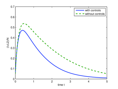
Figure 1: $(I+L_{2})/N$ with and without controls for $\beta=100$, $N=30000$, $\epsilon_{1}=\epsilon_{2}=0.5$, $W_{1}=500$ and $W_{2}=50$.

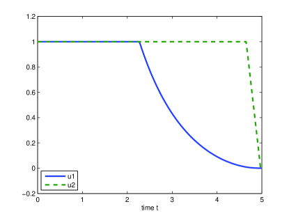
Figure 2: Controls $u_{1}$ and $u_{2}$ for $\beta=100$, $N=30000$, $\epsilon_{1}=\epsilon_{2}=0.5$, $W_{1}=500$, $W_{2}=50$.

We test the relevance of the optimal control strategies, given by controls $u_{1}$ and $u_{2}$, in the reduction of the fraction of active infected individuals $I/N$ and persistent latent individuals $L_{2}/N$. We observe in Figure 3 that both fractions $I/N$ and $L_{2}/N$ are lower when controls are considered, that is, we can conclude that the implementation of the measures to prevent the failure of treatment in active TB infectious individuals $I$ and the increase of number of persistent latent individuals $L_{2}$, that are identified and put under treatment, are good policies for the achievement of our goal. Some of the policies associated to the control $u_{1}$ are the supervision and the support of active TB infectious individuals $I$. It is important to ensure that active TB infectious individuals $I$ complete the treatment, which is difficult due to its duration and second effects. The supervision can be made, however, not only in hospitals but also paying to specialized people to go to patients home. This implies higher monetary cost, that is, greater values for $W_{i}$, which is illustrated in Figures 6–8.

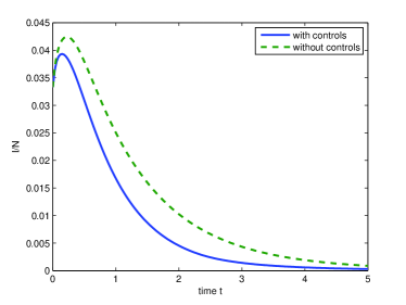
(a) $I/N$ with and without controls

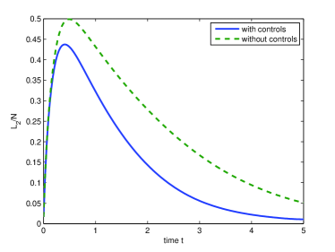
(b) $L_{2}/N$ with and without controls

Figure 3: $I/N$ and $L_{2}/N$, with and without controls, for $\beta=100$, $N=30000$, $\epsilon_{1}=\epsilon_{2}=0.5$, $W_{1}=500$ and $W_{2}=50$.

In what follows, we consider always strategies using controls $u_{1}(t)$ and $u_{2}(t)$ with $t\in[0,5]$. Figure 4 illustrates how optimal control strategies change as the transmission coefficient parameter $\beta$ varies. We consider four different values for $\beta$, $75$, $100$, $150$ and $175$, the other parameters taking the values $N=30000$, $\epsilon_{1}=\epsilon_{2}=0.5$, $W_{1}=500$, and $W_{2}=50$ (the values of the remaining parameters are presented in Table 1). All the values that $\beta$ takes correspond to the case where the disease may become endemic, i.e., $R_{0}>1$. We observe that as the parameter $\beta$ increases, the control $u_{1}$ is at the upper bound for a longer period of time, but the variation on the control $u_{2}$ is not so significant. In Figure 4 (c) one can see that as $\beta$ decreases the fraction of infectious and persistent latent individuals also decreases, as expected.

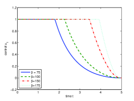
(a) Control $u_{1}$

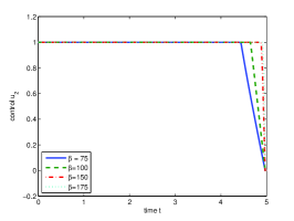
(b) Control $u_{2}$

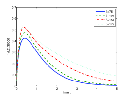
(c) $(I+L_{2})/30000$

Figure 4: Variation of parameter $\beta$ ($\beta=75,100,150,175$).

In Figure 5 the size of the population takes three different values, $30000$, $40000$ and $60000$, and the controls $u_{1}(t)$ and $u_{2}(t)$ are plotted for $t\in[0,5]$. One can conclude that the optimal strategies do not vary significantly: the control $u_{1}$ is at the upper bound during 2.5 years for $N=40000$ and during 2.8 years for $N=60000$, and $u_{2}$ is at the upper bound during 4.7 years for $N=40000$ and during 4.8 years for $N=60000$. On the other hand, the controls $\left(u_{1}(\cdot),u_{2}(\cdot)\right)$ are such that the fraction of infectious and persistent latent individuals $\left(I+L_{2}\right)/N$ does not depend on the size of the population.

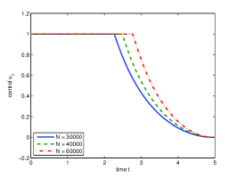
(a) Control $u_{1}$

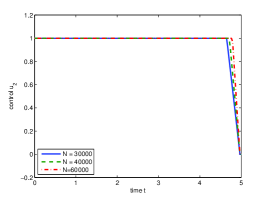
(b) Control $u_{2}$

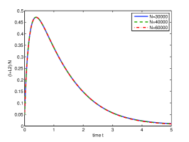
(c) $(I+L_{2})/N$

Figure 5: Different sizes $N$ of population ($N=30000$, $40000$, $60000$) with $\beta=100$, $W_{1}=500$, $W_{2}=50$, $\epsilon_{1}=\epsilon_{2}=0.5$, and the values of the parameters of Table 1.

In Figures 6–8 we present the effect of the weight constants $W_{i}$, $i=1,2$, on the controls, where $\beta=100$, $N=30000$, and $\epsilon_{1}=\epsilon_{2}=0.5$ (and the other parameters are given by Table 1). We assume that the weight constant $W_{1}$ associated with the control $u_{1}$ is greater or equal than the weight constant $W_{2}$ associated with the control $u_{2}$, because the cost associated to $u_{1}$ includes the cost of holding active infected patients $I$ in the hospital or paying people to supervise the patients, assuring that they finish their treatment, and the cost associated to $u_{2}$ is related to the fraction of persistent latent individuals $L_{2}$ that is put under treatment. It is clear that when $W_{1}$ is fixed and $W_{2}$ increases, the amount of $u_{2}$ decreases and $u_{1}$ remains the same (Figure 6). Analogously, when $W_{2}$ is fixed and $W_{1}$ decreases, the amount of $u_{1}$ increases (Figure 7). When the weight constants are equal (Figure 8), both controls vary but, in all the three cases, the optimal control strategies assure the same value for the fraction of infectious and persistent latent individuals. Figure 9 illustrates the situation when we vary the measures of control efficacy $\epsilon_{i}$, $i=1,2$. We consider $\beta=100$, $N=30000$, $W_{1}=500$, $W_{2}=50$, and $\epsilon_{1}=\epsilon_{2}$ with $\epsilon_{i}=0.25;0.5;0.75$, $i=1,2$. We observe that as the efficacy of the controls increase, the control strategies contribute to the minimization of the fraction of infectious and persistent latent individuals.

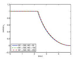
(a) Control $u_{1}$

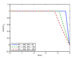
(b) Control $u_{2}$

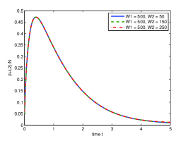
(c) $(I+L_{2})/N$

Figure 6: Variation on the control weights: fix $W_{1}=500$ and vary $W_{2}$ ($W_{2}=50,150,250$).

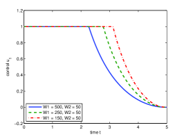
(a) Control $u_{1}$

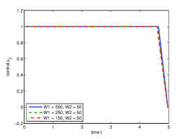
(b) Control $u_{2}$

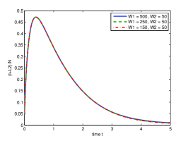
(c) $(I+L_{2})/N$

Figure 7: Fix $W_{2}=50$ and decrease $W_{1}$ ($W_{1}=500,250,150$).

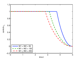
(a) Control $u_{1}$

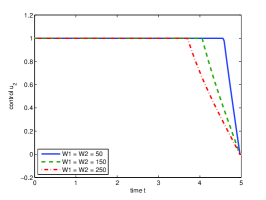
(b) Control $u_{2}$

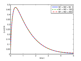
(c) $(I+L_{2})/N$

Figure 8: $W_{1}=W_{2}=50,150,250$.

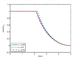
(a) Control $u_{1}$

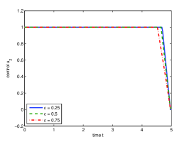
(b) Control $u_{2}$

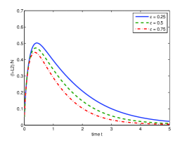
(c) $(I+L_{2})/N$

Figure 9: Variation on $\epsilon_{i}$, $i=1,2$ ($\epsilon_{1}=\epsilon_{2}=0.25;0.5;0.75$).

If we increase the transmission coefficient $\beta$, a different scenario occurs. TB rises and then declines in all of the simulations presented so far. Because TB is clearly already endemic in most relevant settings, we are not before the peak in Figure 3 and Figures 4–9 (c). But if we are now at the point where we are after that peak, then TB is declining anyway in all of the figures. However, if we take, for example, $\beta=200$, this situation does not occur. If we don’t introduce controls, the number of active infected individuals $I$ and persistent latent individuals $L_{2}$ increases significantly, see Figure 10. For these parameter values we have $R_{0}(0,0)=4.4$.

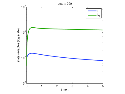
Figure 10: Number of active infected individuals $I$ and persistent latent individuals $L_{2}$, $\beta=200$ and $N=30000$, when no controls are used.

We now show a new situation where the controls have a crucial role: without controls the number of infected increases, while using the optimal control approach the number of infected decreases and remains always in a lower level. Let $N=30000$, $\epsilon_{1}=\epsilon_{2}=0.5$, and $W_{1}=W_{2}=500$. Take, for example, $\beta=250$. If the control measures $u_{1}$ and $u_{2}$ are not implemented, then the number of active infected individuals $I$ increases in all the treatment period. However, if the control measures $u_{1}$ and $u_{2}$ are used (see Figure 11 for the optimal controls) an important decrease of active infected individuals is observed (see Figure 12). Without controls the basic reproduction number is $R_{0}(0,0)=5.5$ and with controls $R_{0}(1,1)=4.4$.

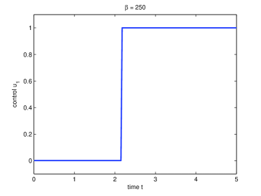
(a) Control $u_{1}$

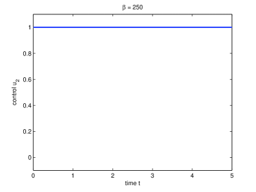
(b) Control $u_{2}$

Figure 11: Controls $u_{1}$ and $u_{2}$ for $\beta=250$; $\epsilon_{1}=\epsilon_{2}=0.5$; $W_{1}=W_{2}=500$; $N=30000$.

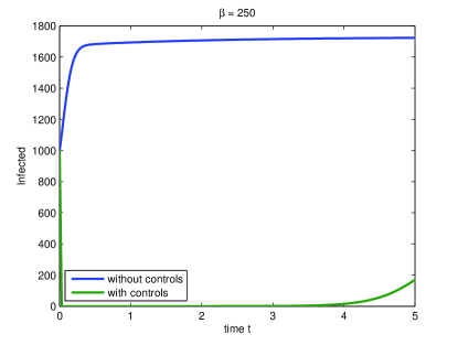
Figure 12: Number of active infected individuals with and without controls.

Other cost functionals could be considered in the optimal control problem, namely a cost $C$ where the category of persistent latent individuals $L_{2}$ is not considered in (7), that is,

$$C(u_{1}(\cdot),u_{2}(\cdot))=\int_{0}^{T}\left[I(t)+\frac{W_{1}}{2}u_{1}^{2}(t)+\frac{W_{2}}{2}u_{2}^{2}(t)\right]dt.$$ (13)

However, in Figures 13 and 14 we observe, for different values of $\beta$, that when we consider the cost functional (7), the fraction of active infectious individuals is lower compared with the case when we consider only active infectious TB individuals $I$ (13).

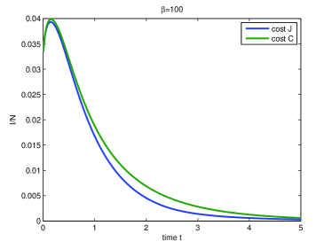
(a) Fraction $I/N$ of infected individuals

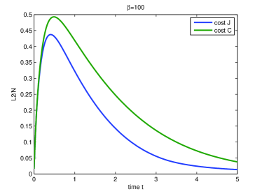
(b) Fraction $L_{2}/N$ of persistent latent individuals

Figure 13: Comparison of active infectious $I$ and persistent latent $L_{2}$ individuals for different cost functionals $J$ and $C$ ($\beta=100$).

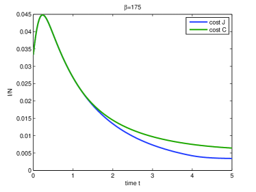
(a) Fraction $I/N$ of infected individuals

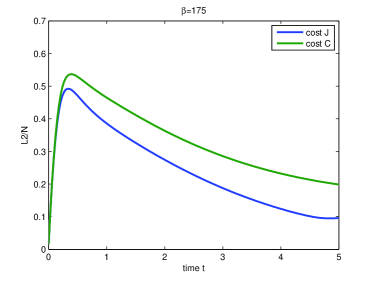
(b) Fraction $L_{2}/N$ of persistent latent individuals

Figure 14: Comparison of active infectious $I$ and persistent latent $L_{2}$ individuals for different cost functionals $J$ and $C$ ($\beta=175$).

Let $N=30000$, $\beta\in\{100,175\}$, $\epsilon_{1}=\epsilon_{2}=0.5$ and $W_{1}=W_{2}=500$. When we compare the controls $u_{1}$ and $u_{2}$ for the cost functionals $J$ and $C$, we observe that a bigger effort is required on the controls when we propose to minimize $I+L_{2}$. If our aim is to minimize the active infected individuals $I$ as well as the cost of the control measures represented by $u_{1}$ (preventive measures applied to active infected individuals for a complete treatment with anti-TB drugs), then the control $u_{1}$ never attains the maximum value and the control measure $u_{2}$ is not required, see Figure 15.

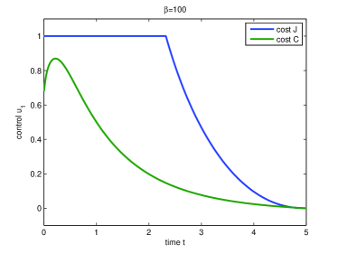
(a) Control $u_{1}$

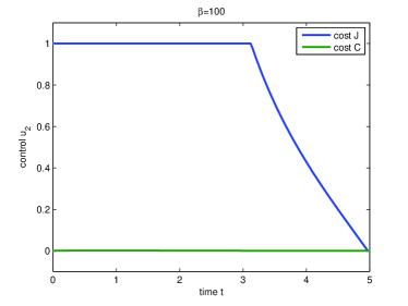
(b) Control $u_{2}$

Figure 15: Comparison of controls $u_{1}$ and $u_{2}$ for different cost functionals $J$ and $C$ ($\beta=100$).

When $\beta=175$, if we want to minimize the cost functional $C$ then the control $u_{1}$ attains the maximum value for approximately 1.1 years; if we want to minimize the cost functional $J$ then the control $u_{1}$ attains the maximum value for approximately 3.9 years. Analogously to the case $\beta=100$, for $\beta=175$ the control measure $u_{2}$ is not required when we wish to minimize $C$, see Figure 16.

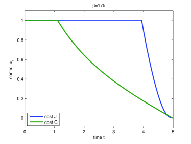
(a) Control $u_{1}$

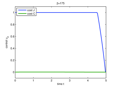
(b) Control $u_{2}$

Figure 16: Comparison of controls $u_{1}$ and $u_{2}$ for different cost functionals $J$ and $C$ ($\beta=175$).

The bigger effort on the control measures associated to the cost functional $J$ is justified by a reduction on the fraction of active infected individuals $I$ and persistent latent individuals $L_{2}$, when compared to the case of minimizing $C$, see Figure 13. This reduction is more significant if we consider $\beta=175$, see Figure 14.

Finally, we can compare the effect of the implementation of two controls strategies: apply only the control $u_{1}$ (supervision and support of TB infectious individuals $I$); and apply simultaneously $u_{1}$ and $u_{2}$. The treatment of persistent latent individuals $L_{2}$, for example with a prophylactic vaccine, is not so usual as the treatment of active infectious individuals, which is one of the measures proposed by the Direct Observation Therapy (DOT) of World Health Organization (WHO), but is a valid TB treatment strategy [1, 8]. Observing Figure 17, we conclude that each control $u_{1}$ and $u_{2}$ implies a reduction on the respective fraction of the population, $I$ and $L_{2}$. Moreover, if we choose to minimize the cost function (7), then the best choice is to apply both controls simultaneously, since the implementation of control $u_{2}$ does not imply a reduction on the fraction of active infectious individuals. For this reason, if we choose to minimize the cost function (13), then the best control strategy is to implement only control $u_{1}$.

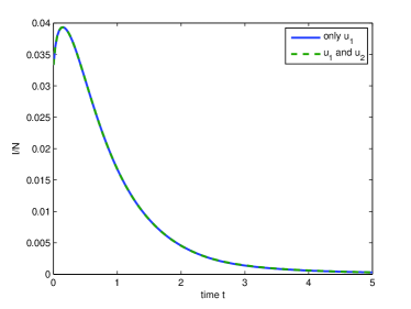
(a) Fraction $I/N$ of infected individuals

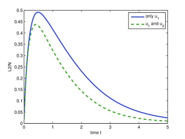
(b) Fraction $L_{2}/N$ of persistent latent individuals

Figure 17: Comparison between applying only control $u_{1}$ and applying the two controls $u_{1}$ and $u_{2}$ simultaneously, with $\beta=100$, $\epsilon_{1}=\epsilon_{2}=0.5$, $W_{1}=500$, $W_{2}=50$, and $N=30000$.

6 Conclusion

The incidence rates of TB have been declining since 2004 worldwide, namely due to prevention and treatment policies that have been applied in the last years [26]. Mortality rates, at global level, fell down around 35% between 1990 and 2009, and if the current rate of decline is sustained, by 2015 the target of a 50% reduction can be achieved. The reduction of mortality and incidence rates depend on the effort at country level to implement control policies. Examples of policies that had a great success in WHO’s six regions are the DOTS strategy (1995-2005) and its sucessor Stop TB launched in 2006 (see [26] for further details). In this paper we study a mathematical model for TB proposed in [12], from the optimal control point of view. Optimal time-dependent prevention policies, that consider the execution cost, are proposed. We tried different numerical approaches and we observed that the results are the same, independently of the method used. In particular, two approaches have been tried: direct and indirect. The direct methods discretize the problem turning it into a nonlinear optimization problem. Indirect methods use the Pontryagin Maximum Principle [18] as a necessary condition to find the optimal curve for the respective control: we substitute (12) into (11) and the obtained system of five equations is solved numerically together with the five equations of system (1). Figures 1 and 2 show that when controls are considered, the optimal policies provide a reduction of 1230 active infectious and persistent latent individuals. The cost execution of the control policies related to control $u_{1}$ is assumed to be greater or equal to the one related to control $u_{2}$ (see Section 5). Figures 7 and 8 show that when the cost of implementation of control policies related to control $u_{1}$ decreases, the amount of $u_{1}$ increases, and when the cost of implementation of control policies related to control $u_{2}$ decreases, the amount of $u_{2}$ increases. We considered different values for the transmission coefficient parameter $\beta$ corresponding to the case where the disease may become endemic. We observe that as the transmission coefficient increases, the period of time that the control $u_{1}$ (associated to the effort that prevents the failure of treatment of active infectious individuals) is at the upper bound also increases, as well as the fraction of active infectious and persistent latent individuals (Figure 4). We assume that the total population $N$ is constant and Figure 5 illustrates that optimal control strategies do not vary significantly when different sizes of population are taken. As we can see in Figure 9, the measures of the efficacy of control policies $\epsilon_{1}$ and $\epsilon_{2}$ strongly influence the effect of the control policies related to $u_{1}$ and $u_{2}$ on the minimization of the number of active infectious and persistent latent individuals.

As future work, it would be interesting to consider different values for the parameters $\tau_{1}$ and $\tau_{2}$, and observe the variations on the optimal control strategies. In addition, we intend to study optimal control strategies for the minimization of the fraction of active infectious and/or persistent latent individuals, when susceptibility to reinfection of treated individuals differs from that of latent: $\sigma_{R}<\sigma$ or $\sigma_{R}>\sigma$. Another direction of research consists to study TB/HIV co-infections.

References

- [1] L. J. Abu-Raddad, L. Sabatelli, J. T. Achterberg, J. D. Sugimoto, I. M. Longini, C. Dye, M. E. Halloran, Epidemiological benefits of more-effective tuberculosis vaccines, drugs, and diagnostics, Proc. Natl. Acad. Sci. U.S.A. 106 (2009), no. 33, 13980–13985.
- [2] A. Bandera, A. Gory, L. Catozzi, A. Degli Esposti, G. Marchetti, C. Molteni, G. Ferrario, L. Codecasa, V. Penati, A. Matteelli, F. Franzetti, Molecular epidemiology study of exogenous reinfection in an area with a low incidence of tuberculosis, J. Clin. Microbiol. 39 (2001), no. 6, 2213–2218.
- [3] S. Bowong, Optimal control of the transmission dynamics of tuberculosis, Nonlinear Dynam. 61 (2010), no. 4, 729–748.
- [4] J. A. Caminero, M. J. Pena, M. I. Campos-Herrero, J. C. Rodriguez, O. Afonso, C. Martin, J. M. Pavón, M. J. Torres, M. Burgos, P. Cabrera, P. M. Small, D. A. Enarson, Exogenous reinfection with tuberculosis on a European island with a moderate incidence of disease, Am. J. Respir. Crit. Care Med. 163 (2001), no. 3, 717–720.
- [5] C. Castillo-Chavez, Z. Feng, To treat or not to treat: the case of tuberculosis, J. Math. Biol. 35 (1997), no. 6, 629–656.
- [6] L. Cesari, Optimization — Theory and Applications. Problems with Ordinary Differential Equations, Applications of Mathematics 17, Springer-Verlag, New York, 1983.
- [7] N. Chitnis, J. M. Hyman, J. M. Cushing, Determining important parameters in the spread of malaria through the sensitivity analysis of a mathematical model, Bull. Math. Biol. 70 (2008), no. 5, 1272–1296.
- [8] T. Cohen, M. Lipsitch, R. P. Walensky, and M. Murray, Beneficial and perverse effects of isoniazid preventive therapy for latent tuberculosis infection in HIV-tuberculosis coinfected populations, Proc. Natl. Acad. Sci. U.S.A. 103 (2006), no. 18, 7042–7047.
- [9] Y. Emvudu, R. Demasse, D. Djeudeu, Optimal control of the lost to follow up in a tuberculosis model, Comput. Math. Methods Med. 2011 (2011), Art. ID 398476, 12 pp.
- [10] Z. Feng, C. Castillo-Chavez, A. F. Capurro, A model for tuberculosis with exogenous reinfection, Theor. Pop. Biol. 57 (2000), no. 3, 235–247.
- [11] W. H. Fleming, R. W. Rishel, Deterministic and Stochastic Optimal Control, Springer Verlag, New York, 1975.
- [12] M. G. M. Gomes, P. Rodrigues, F. M. Hilker, N. B. Mantilla-Beniers, M. Muehlen, A. C. Paulo, G. F. Medley, Implications of partial immunity on the prospects for tuberculosis control by post-exposure interventions, J. Theoret. Biol. 248 (2007), no. 4, 608–617.
- [13] K. Hattaf, M. Rachik, S. Saadi, Y. Tabit, N. Yousfi, Optimal control of tuberculosis with exogenous reinfection, Appl. Math. Sci. (Ruse) 3 (2009), no. 5-8, 231–240.
- [14] E. Jung, S. Lenhart, Z. Feng, Optimal control of treatments in a two-strain tuberculosis model, Discrete Contin. Dyn. Syst. Ser. B 2 (2002), no. 4, 473–482.
- [15] Q. Kong, Z. Qiu, Z. Sang, Y. Zou, Optimal control of a vector-host epidemics model, Math. Control Relat. Fields 1 (2011), no. 4, 493–508.
- [16] M. E. Kruk, N. R. Schwalbe, C. A. Aguiar, Timing of default from tuberculosis treatment: a systematic review, Trop. Med. Int. Health 13 (2008), no. 5, 703–712.
- [17] S. Lenhart, J. T. Workman, Optimal control applied to biological models, Chapman & Hall/CRC, Boca Raton, FL, 2007.
- [18] L. Pontryagin, V. Boltyanskii, R. Gramkrelidze, E. Mischenko, The Mathematical Theory of Optimal Processes, Wiley Interscience, 1962.
- [19] H. S. Rodrigues, M. T. T. Monteiro, D. F. M. Torres, Dynamics of dengue epidemics when using optimal control, Math. Comput. Modelling 52 (2010), no. 9-10, 1667–1673. arXiv:1006.4392
- [20] H. S. Rodrigues, M. T. T. Monteiro, D. F. M. Torres, A. Zinober, Dengue disease, basic reproduction number and control, Int. J. Comput. Math. 89 (2012), no. 3, 334–346. arXiv:1103.1923
- [21] P. M. Small, P. I. Fujiwara, Management of tuberculosis in the United States, N. Engl. J. Med. 345 (2001), no. 3, 189–200.
- [22] K. Styblo, State of art: epidemiology of tuberculosis, Bull. Int. Union Tuberc. 53 (1978), 141–152.
- [23] K. Styblo, Epidemiology of tuberculosis: epidemiology of tuberculosis in HIV prevalent countries, Royal Netherlands Tuberculosis Association, 1991.
- [24] A. van Rie, R. Warren, M. Richardson, T. C. Victor, R. P. Gie, D. A. Enarson, N. Beyers, P. D. van Helden, Exogeneous reinfection as a cause of recurrent tuberculosis after curative treatment, N. Engl. J. Med. 341 (1999), 1174–1179.
- [25] WHO, Treatment of tuberculosis guidelines, Fourth edition, WHO Report, Geneva, 2010.
- [26] WHO, Global Tuberculosis Control, WHO Report, Geneva, 2011.
- [27] https://projects.coin-or.org/Ipopt
- [28] http://www.ampl.com
- [29] http://tomdyn.com