Core-excitation three-cluster model description of ⁸He and ¹⁰He

Abstract

We introduce a new model applying to the core-nucleus and two-neutron system. The Faddeev equations of ⁶He-n-n and ⁸He-n-n systems for ⁸He and ¹⁰He are solved, respectively. The potential of the subsystem in the model has been determined to make a coupling both of the ground state and the excited one inside the core nucleus. By a similar mechanism the three-nucleon system is solved with the three-body force originating from an isobar excitation of the nucleon. Inputting only the information of subsystem energy levels and widths we get the coupling constants of rank 1 Yamaguchi potential between the core nucleus and neutron. We calculate the Faddeev three-cluster equations to obtain the low-lying energy levels of ⁸He and ¹⁰He. The 1^- state of ¹⁰He, which has not been detected yet in experiments, is located in the energy level between the 0⁺ and 2⁺ states.

I I. INTRODUCTION

Due to developments of experimental technique, our knowledge of unstable nuclei has been increasing rapidly. Experimental researchers have recently reported a lot of events. Here neutron-rich nuclei are good targets for studying interesting phenomena, e.g., clustering, halos, deformation, dineutron correlation, etc. In order to look for these properties which differ from ordinary shell model study, one may need to employ cluster model calculations. However, the interactions between clusters are usually very complex, except for the $\alpha$ cluster model treated as the resonating group method. According to ab initio calculations, there are at most four-body calculationsKamada et al. (2001). Four-nucleon scattering has been solved by the Faddeev-Yakubovsky formalism using the realistic nucleon-nucleon force including the three-body forceViviani et al. (2011). Beyond the four-nucleon system there are computational difficulties because of limited memory size and CPU time. Nevertheless, the Green’s function Monte Carlo simulation is very promising. Recent calculations show many energy spectra up to A = 9 Pastore et al. (2013).

There are some microscopic or effective theoretical approaches. For instance, the cluster orbital shellmodel (COSM), complex scaling method (CSM)Aguilar and Combes (1971), and the method of analytic continuation in the coupling constant (ACCC)Kukulin et al. (1979) describe ⁹He and ¹⁰He nuclei by their core-nucleus + valence-neutrons model Aoyama et al. (1997); Aoyama (2002). Systematic studies from ⁵He to ⁸He are reported on the basis of the tensor-optimized shell model (TOSM) Myo et al. (2011) using a bare nucleon-nucleon interaction, of which the short-range correlation is treated by the unitary correlation operator method (UCOM) Neff and Feldmeier (2003).

On the other hand, the three-cluster model of the Faddeev theory has been applied to the low-lying energy states of the ⁶Li nucleus as $\alpha$ + n + p three-body system using nonlocal separable interactions Eskandarian and Afnan (1992). In the case of T=1 the isotope ⁶He the binding energy and widths of the resonance for the ground state J^π=0⁺ and the resonance state J^π=2⁺ agree with experiment. By the same scheme we have also been investigating other exotic nucleus ${}^{9}_{\Lambda}$Be of $\alpha$ + $\alpha$ + $\Lambda$ three-body systemOryu et al. (2000); Cravo et al. (2002).

In the next section we will introduce a new model calculation based on the Faddeev theory. The three-body system is treated as the cluster model consisting of core-nucleus + n + n to investigate ⁸He and ¹⁰He nuclei. ^6,8He are so-called Borromean nuclei and ¹⁰He is also regarded as the Borromean nucleus because the energy level of the ground state is much closer to the three-body breakup threshold. It is often considered that the core-nucleus of the three-body model deals with only the ground state core-nucleus. However, in our model not only the ground state core-particle but also an excited state core-nucleus are adopted. The idea Koike (2003) is also found in the case of the 3-nucleon system, in which some of nucleons become delta isobar in ³HePe${\tilde{\rm n}}$a et al. (1990).

Preliminary calculations have been carried out Uzu et al. (2007); Yamaguchi et al. (2007). Because the excited state J^π=${1\over 2}^{-}$ of ⁷He was not found in the experiment, in the former work ⁸He ground state coluld not be described accurately. Using the presence of the excited state in the experimentSkaza et al. (2006) we recalculate with the new data of ⁷He. Our theoretical prediction will be demonstrated in case of ⁸He and ¹⁰He nuclei in section 3. The conclusion is given in section 4.

II II. A new three-cluster model

In the framework of the Faddeev theory the three-body equations were represented as the Alt-Grassberger-Sandhas (AGS) equations using a separable potential of NN interactionLovelace (1964). The AGS equations are used in many three-body systems. It has succeeded in calculation of a three-body breakup process for the $\alpha$- n -p system first Koike (1978). Recently the study of the system has progressed well Deltuva (2006). The system was often investigated and the calculation of the resonance states T=1 without Coulomb force are discussed just corresponding to the case of ⁶He nucleus. We verified the former work Eskandarian and Afnan (1992) and the energy level of the ground state J^π=0⁺ from the threshold of $\alpha$ +2n is obtained as – 0.56 MeV vs. data – 0.973 MeV. The energy level of the first excited state J^π=2⁺ is also obtained as 0.95 MeV ( $\Gamma$ =0.3MeV) vs. data 0.824MeV ( $\Gamma$ =0.113MeV)Tilley et al. (2002). The separable potential is very primitive, nevertheless, these calculations encourage us to start neutron-rich study.

On the other hand, the research in three-nucleon scattering has made great progress according to the three-body forceGlöckle et al. (1996); Witala et al. (2011). It is considered that the fundamental origin of the three-body forces comes from the delta excitation, or inner excitation, of nucleonFujita and Miyazawa (1957). Study of the three-nucleon force is progressing recently centering on the chiral symmetry which QCD Lagrangian possessesEpelbaum et al. (2008); Epelbaum (2013).

If the idea of the inner excitation is applied to the case of neutron-rich nuclei, more precise theoretical expectations would be possible taking into consideration the inner excitation of the core-cluster which constitutes the nucleusKoike (2003). This idea has a similarity to the delta isobar excitation in the three-nucleon system Pe${\tilde{\rm n}}$a et al. (1990). Illustrations of the model which we imagine, are shown in Fig. 1. Labels ”G” of Fig. 1 (a) and ”X” of Fig. 1 (b) mean the names of the ground state core-nucleus and the excited state one, respectively.

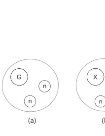
Figure 1: Illustration of core-excitation cluster. The core-cluster of the ground state and excited state are labeled ”G” and ”X”, respectively. Neutrons are also labeled ”n”.

The Hilbert space $\cal H$ of the model consists of two Hilbert ones ;

$${\cal H}={\cal H}(G)+⃝{\cal H}(X).$$ (1)

Using the word of wave function, we have

$$|\Psi\rangle=|G\rangle|\Psi_{G}\rangle+|X\rangle|\Psi_{X}\rangle,$$ (2)

where $|G\rangle$ and $|X\rangle$ are orthonormal basis to distinguish their spaces,

$$\langle G|G\rangle=\langle X|X\rangle=1,~{}~{}~{}~{}\langle G|X\rangle=\langle X|G\rangle=0.$$ (3)

The free Hamiltonian $\hat{H}_{0}^{2clust.}$ of the subsystem consisting of the core-nucleus and neutron is represented as

$$\hat{H}_{0}^{2clust.}|G\rangle\equiv{p^{2}\over 2\nu}|G\rangle,$$ (4)

$$\hat{H}_{0}^{2clust.}|X\rangle\equiv(\delta m+{p^{2}\over 2\nu})|X\rangle,$$ (5)

where $p$ and $\nu$ are the relative momentum and the reduced mass between the core-nucleus and neutron, respectively. The mass difference $\delta m$ is the energy level shift of the ground core-nucleus and the excited one.

II.1 Two-Body interaction

In our model the potential of two-cluster system has a rank 1 separable Yamaguchi form using a simple formfactor $g(p)$. For instance, the neutron-neutron potential of ¹S₀ partial wave is given as

$$V_{nn}(p,p^{\prime})=-\gamma_{nn}^{2}g_{nn}(p)g_{nn}(p^{\prime})$$ (6)

with

$$g_{nn}(p)={1\over p^{2}+\beta_{nn}^{2}},$$ (7)

where we choose parameters as $\beta_{nn}$=1.1648 fm^-1 and $\gamma_{nn}^{2}=$0.3943fm^-3 from Eskandarian and Afnan (1992).

Let us introduce a new form factor $h$, which is combined with the partial waves $|l_{I}S_{I}j_{I}\rangle$ and the particle basis $|I\rangle$;

$$\langle p|h\rangle=\sum_{I=G,X}\sum_{l_{I},S_{I},j_{I}}\gamma_{In;l_{I},S_{I},j_{I}}~{}g_{In;l_{I},S_{I},j_{I}}(p)|l_{I}S_{I}j_{I}\rangle|I\rangle$$ (8)

(9)

with

$$g_{In;l_{I},S_{I},j_{I}}(p)={p^{l_{I}}\over(p^{2}+\beta_{In;l_{I},S_{I},j_{I}}^{2})^{l_{I}+1}}$$ (10)

where $l_{I}$, $S_{I}$ and $j_{I}$ are angular momentum, total spin and total angular momentum of 2-body subsystem ($j_{I}=l_{I}+S_{I}$), respectively. The core-nuclei neutron potential $V$ is given by the formfactor $h$,

$$\hat{V}=-|h\rangle\langle h|.$$ (11)

However, the neutron-neutron (nn) potential $\hat{V}_{nn}$differs from this form, one writes it as

$$\hat{V}_{nn}=-|g_{nn}\rangle\gamma_{nn}^{2}\langle g_{nn}|\{|G\rangle\langle G|+|X\rangle\langle X|\}.$$ (12)

Apparently the potential $\hat{V}_{nn}$ is not coupled between $|G\rangle$ and $|X\rangle$.

When the core-nucleus spin has the ground state 0⁺ and the excited state 2⁺, there are $S_{G}={1\over 2}$ and, $S_{X}={3\over 2}$ and ${5\over 2}$, respectively. If one takes the same number for the parameter $\beta$ the potentials of $S_{X}={3\over 2}$ and $S_{X}={5\over 2}$ differ only in the coupling constants. The degenerated coupling constant $\gamma_{In;l_{I},j_{I}}^{2}$ could be introduced;

$$\gamma_{Gn;l_{G},j_{G}}^{2}\equiv\gamma_{Gn;l_{G},{1\over 2},j_{G}}^{2},$$ (13)

$$\gamma_{Xn;l_{X},j_{X}}^{2}\equiv\gamma_{Xn;l_{X},{3\over 2},j_{X}}^{2}+\gamma_{Xn;l_{X},{5\over 2},j_{X}}^{2}.$$ (14)

According to the separable scheme the t-matrix $t(p,p^{\prime};E_{2})$

$$t_{In;l_{I},S_{I},j_{I},I^{\prime}n;l_{I}^{\prime},S_{I}^{\prime},j_{I}^{\prime}}(p,p^{\prime};E_{2})$$ (15)

$$\equiv\langle I|\langle l_{I}S_{I}j_{I}|\langle p|h\rangle\tau(E_{2})\langle h|p^{\prime}\rangle|l_{I}^{\prime}S_{I}^{\prime}j_{I}^{\prime}\rangle|I^{\prime}\rangle$$ (16)

fulfills the Lippmann-Schwinger equation with resulting

$$\tau(E_{2})=-1-\tau(E_{2})\langle h|\hat{G}_{0}^{2clust.}(E_{2})|h\rangle.$$ (17)

In order to determine these coupling constants $\gamma$ in Eq. (9) we introduce the following natural assumption. If the subsystem has no bound state (Borromean nuclei is just in this case) but has some resonance states, the propagator $\tau(E_{2})$ must be diverged at the resonance energy $E_{2}=E_{2}^{res}$ which has a real part $E_{2}^{(r)}$ and width $\Gamma$. Under the condition $\tau(E_{2})=\infty$ Eq. (17) becomes

$$1+\gamma_{Gn;l_{G},j_{G}}^{2}\langle g_{Gn;l_{G},j_{G}}|{1\over E_{2}^{res}-\hat{p}^{2}/2\nu+i\epsilon}|g_{Gn;l_{G},j_{G}}\rangle$$ (18)

$$+\gamma_{Xn;l_{X},j_{X}}^{2}\langle g_{Xn;l_{X},j_{X}}|{1\over E_{2}^{res}-\delta m-\hat{p}^{2}/2\nu+i\epsilon}|g_{Xn;l_{X},j_{X}}\rangle$$ (19)

$$=0$$ (20)

Approximately the resonance state occurs only two channel and there is assumed to be no absorption channel, we expect these coupling constants are a real number. Consequently, the condition leads to 2 conditions (real part and imaginary one) to subtract 2 unknown parameters $\gamma_{G}$ and $\gamma_{X}$.

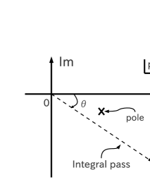
Figure 2: Integral pass of Eq. (20). In Riemann complex sheet of the variable $p$ the integral pass is taken as the dashed line below the resonance pole.

As shown in Fig. 2 one needs to take the integral pass of Eq. (20), because the resonance pole is located on physical Riemann sheet at $p=p_{pole}$ with $p_{pole}^{2}=2\nu E_{2}^{res}$.

In order to apply these potential to the three-body system, we must resolve the degeneracy of $S_{X}$. Following a natural way of thinking the weight of the couplings will be taken from the degree of multiplicity under the condition of (14) ,

$$\gamma_{Xn;l_{X},S_{X},j_{X}}=\sqrt{2S_{X}+1\over 10}\gamma_{Xn;l_{X},j_{X}}.$$ (21)

We will show these coupling constants of ⁶He-n and ⁸He-n in section III.

II.2 Three-body integral equation

The AGS equations are well-established Afnan and Thomas (1974), therefore, we will not repeat the same part of Ref. Eskandarian and Afnan (1992). The following explanation is an additional part because of the extension of core-excitation channel ($G$ or $X$) and the definition of the wave function.

The total wave function $|\Psi^{J^{\pi}T}\rangle$ with the total angular momentum $J$, the parity $\pi$, and total isospin $T$ consists of the Faddeev components $\psi^{J^{\pi}T}$ labeled by particle-channel $\alpha$, $\beta$ and $\gamma$;

$$|\Psi^{J^{\pi}T}\rangle=|\psi_{\alpha}^{J^{\pi}T}\rangle+|\psi_{\beta}^{J^{\pi}T}\rangle+|\psi_{\gamma}^{J^{\pi}T}\rangle.$$ (22)

The AGS equations for the Faddeev component is given by

$$|\psi_{\alpha}^{J^{\pi}T}\rangle = G_{0}t_{\alpha}\sum_{\beta\not=\alpha}|\psi_{\beta}^{J^{\pi}T}\rangle$$ (23)

$$= G_{0}|h_{\alpha}\rangle\tau_{\alpha}\langle h_{\alpha}|\sum_{\beta\not=\alpha}|\psi_{\beta}^{J^{\pi}T}\rangle.$$ (24)

The reduced wave function $f_{I;\tilde{K}_{\alpha}}^{J^{\pi}T}(q_{\alpha})$ is defined by

$$\sum_{I=G,X}\langle I|\langle\tilde{K}_{\alpha}|\langle q_{\alpha}|f_{\alpha}^{J^{\pi}T}\rangle=\langle q_{\alpha}|f_{\tilde{K}_{\alpha}}^{J^{\pi}T}\rangle=f_{\tilde{K}_{\alpha}}^{J^{\pi}T}(q_{\alpha})$$ (25)

$$\equiv\sum_{I=G,X}\gamma_{In;l_{\alpha},j_{\alpha}}\langle g_{In;l_{\alpha}{j}_{\alpha}}|\sum_{\beta\not=\alpha}|\psi_{I;\beta}^{J^{\pi}T}\rangle,$$ (26)

where $q_{\alpha}$ is the Jacobi momentum designating the momentum of the particle labeled by $\alpha$ relative to the ($\beta\gamma$) pair. The index $K_{\alpha}=\{t_{\alpha},j_{\alpha},S_{\alpha},l_{\alpha},{\cal S}_{\alpha},{\cal L}_{\alpha},I\}$ is defined as the quantum numbers that label the different three-body channels J^π T. The index $\tilde{K}_{\alpha}=\{t_{\alpha},j_{\alpha},l_{\alpha},{\cal S}_{\alpha},{\cal L}_{\alpha}\}$ is also defined because of the degeneration of $S_{\alpha}$ and $I$.

Here, for the sake of unifying the notation the related coupling constant $\gamma_{nn}$ is also written as $\gamma_{In;l_{\alpha},j_{\alpha}}$ when the spectator of the particle channel $\alpha$ is the core-nucleus. The following angular momentum and isospin coupling scheme is given as

$$S_{\alpha}=s_{\beta}+s_{\gamma},~{}~{}~{}j_{\alpha}=l_{\alpha}+S_{\alpha},~{}~{}~{}t_{\alpha}=\tau_{\beta}+\tau_{\gamma},$$ (27)

$${\cal S}_{\alpha}=j_{\alpha}+s_{\alpha},~{}~{}~{}J={\cal L}_{\alpha}+{\cal S}_{\alpha},~{}~{}~{}T=t_{\alpha}+\tau_{\alpha}.$$ (28)

Here, $s_{\beta}$ and $\tau_{\beta}$ refer to the spin and isospin of the particle labeled by $\beta$, $l_{\alpha}$ refers to the relative orbital angular momentum of the ($\beta\gamma$) pair, ${\cal S}_{\alpha}$ is the channel spin; and ${\cal L}_{\alpha}$ is the orbital angular momentum of the spectator particle $\alpha$ relative to the ($\beta\gamma$) pair.

The AGS equations (24) are modified into equations for the reduced wave functions;

$$f_{\tilde{K}_{\alpha}}^{J^{\pi}T}(q_{\alpha})$$ (29)

$$=\sum_{I,I^{\prime}}\sum_{\tilde{K}_{\gamma}}\int_{0}^{\infty}dq_{\gamma}q^{2}_{\gamma}Z_{I;\tilde{K}_{\alpha},I^{\prime};\tilde{K}_{\gamma}}^{J^{\pi}T}(q_{\alpha},q_{\gamma};E)$$ (30)

$$\times\tau_{l_{\gamma}{j}_{\gamma}}(E-\epsilon_{\gamma}(q_{\gamma}))\ f_{\tilde{K}_{\gamma}}^{J^{\pi}T}(q_{\gamma}),$$ (31)

where the integral kernel $Z_{I;K_{\alpha},I^{\prime};K_{\beta}}^{J^{\pi}T}$ is defined by

$$Z_{I;\tilde{K}_{\alpha},I^{\prime};\tilde{K}_{\beta}}^{J^{\pi}T}(q_{\alpha},q_{\beta};E)\equiv$$ (32)

$$\bar{\delta}_{\alpha\beta}~{}\delta_{II^{\prime}}~{}\gamma_{In;l_{\alpha},j_{\alpha}}~{}\gamma_{I^{\prime}n;l_{\beta},j_{\beta}}$$ (33)

$$\times\langle g_{I;l_{\alpha}{j}_{\alpha}};q_{\beta}K_{\beta}JT|G_{0}^{(I)}|g_{I^{\prime};l_{\beta}{j}_{\beta}};q_{\beta}K_{\beta}JT\rangle~{}~{}$$ (34)

and $\epsilon_{\gamma}(q_{\gamma})$ is ${q_{\gamma}^{2}\over 2\mu_{\gamma}}$, and $E$ is a total energy of the three-body c.m. system. Eq. (34) is only changed with the parts of $\delta_{II^{\prime}}$ and $\gamma$ from Eq. (13) of Eskandarian and Afnan (1992). In addition, the free three-body Green’s function $G_{0}$ can be written as

$$G_{0}^{(G)}\equiv\langle G|\hat{G}_{0}|G\rangle={1\over E-p_{\alpha}^{2}/(2\nu_{\alpha})-q_{\alpha}^{2}/(2\mu_{\alpha})+i\epsilon},$$ (35)

$$G_{0}^{(X)}\equiv\langle X|\hat{G}_{0}|X\rangle$$ (36)

$$={1\over E+\delta m-p_{\alpha}^{2}/(2\nu_{\alpha})-q_{\alpha}^{2}/(2\mu_{\alpha})+i\epsilon},$$ (37)

where the reduced mass $\nu_{\alpha}$ and $\mu_{\alpha}$ are $m_{\beta}m_{\gamma}/(m_{\beta}+m_{\gamma})$ and $m_{\alpha}(m_{\beta}+m_{\gamma})/(m_{\alpha}+m_{\beta}+m_{\gamma})$, respectively.

In order to find out the three-body bound state or resonance state we regard the AGS equations of Eq. (31) as the eigen value equation

$$\eta\vec{\psi}={\cal K}(E)\vec{\psi}$$ (38)

where $\eta$ and ${\cal K}(E)$ are the eigen value and the integral kernel $Z(E)\tau$ in Eq. (31), respectively. We need to search for $E$ under a constraint $\eta=1$. Our basic technique is based on the Gauss - Seidel method to solve the eigen value equation. The typical iteration of the procedure is a few hundred times to reach the stable solutions. Performance of the integral for the complex momentum $q_{\gamma}$ takes the integral pass as well as 2-body momentum $p$ shown in Fig. 2. The contour deformation angle $\theta$ is defined

$$p_{\rm complex}\equiv p\exp(-i\theta),q_{\rm complex}\equiv q\exp(-i\theta)$$ (39)

The accuracy of the calculation is sufficiently saved within $\theta\leq{\pi\over 3}$.

III III. Numerical results

We applied the above-mentioned scheme to the core-nucleus+2n systems of ⁸He and ¹⁰He. The results of these systems are separately demonstrated in the next subsections.

III.1 ⁸He nucleus

We treat, here, ⁸He as the ⁶He-n-n three-body system. The energy shift $\delta m$ between the ground state $G$ and the first excited state $X$ of the core-nucleus ⁶He is 1.8 MeV. There are low-lying three resonance states in ⁷He, which are submitted J^π=$({3\over 2})^{-}$ (g.s.;$\Gamma_{cm}$=0.150$\pm$0.020 MeVTilley et al. (2002)), J^π=$({1\over 2})^{-}$ ($E_{x}=$0.9$\pm$0.5 MeV, $\Gamma_{cm}$=1.0$\pm$0.9 MeVSkaza et al. (2006) ) and J^π=$({5\over 2})^{-}$ ($E_{x}=$2.92 $\pm$ 0.09 MeV, $\Gamma_{cm}$=1.990 $\pm$ 0.170 MeV)Tilley et al. (2002). The energy level of the ground state is 0.445 MeV Tilley et al. (2002) from the threshold of ⁶He and neutron, we have each $E_{2}^{res.}$ in Table 1. Using these experimental data we list the coupling constants $\gamma_{I}^{2}$ obtained by solving our model equations (20). For the sake of simplicity the reduced mass $\nu$ is ${6\over 7}m_{N}$ with nucleon mass $m_{N}=$939 MeV.

Table 1: Parameters for ⁶He(0⁺)-n + ⁶He(2⁺)-n potential. The resonance energies are measured from the ⁶He+n threshold. The strengths $\gamma^{2}$ are in unit of fm^-5 for P wave, and fm^-7 for F wave. The parameters $\beta_{G}$ and $\beta_{X}$ are commonly taken 1.5166 fm^-1. ($\beta_{nn}$= 1.1648 fm^-1)

$E_{2}^{res}$ [MeV]	partial wave	$l_{G}$	$\gamma_{G}^{2}$	$l_{X}$	$\gamma_{X}^{2}$
0.445 – i 0.075 Tilley et al. (2002)	2P3/2+4,6P3/2	1	4.1655	1	6.1580
1.345 – i 0.5 Meister et al. (2002); Skaza et al. (2006)	2P1/2+4P1/2	1	5.3966	1	4.0418
3.37 –i 0.995 Tilley et al. (2002)	2F5/2+4,2P5/2	3	116.80	1	7.6144
nn channel	1S0	0	0.3943	0	0.3943

The possible quantum numbers of 3-body partial wave of J^π=0⁺ are listed in table 2. There are 10 channels for J^π=0⁺ ground state of ⁸He, and 32 channels for J^π=2⁺. In table 3 our theoretical predictions are demonstrated with the recent experimental data. Energy levels are reasonably well obtained to describe the data, however, there is a tendency of large width.

Table 2: Set of the quantum numbers for J^π=0⁺ state of ⁸He nucleus. The quantum numbers for the particle channel $\alpha$=3 is obtained from $\alpha$=1 by only cyclically label replacing $s_{\alpha}\to s_{\beta}\to s_{\gamma}\to s_{\alpha}$.

$K_{\alpha}$	$\tilde{K}_{\alpha}$	$\alpha$	I	${\cal L}_{\alpha}$	${\cal S}_{\alpha}$	$j_{\alpha}$	$l_{\alpha}$	$S_{\alpha}$	$s_{\alpha}$	$s_{\beta}$	$s_{\gamma}$
1	1	1	G	1	1	3/2	1	1/2	1/2	1/2	0
2	1	1	X	1	1	3/2	1	3/2	1/2	1/2	2
3	1	1	X	0	0	3/2	1	5/2	1/2	1/2	2
4	2	1	G	0	0	1/2	1	1/2	1/2	1/2	0
5	2	1	X	0	0	1/2	1	3/2	1/2	1/2	2
6	3	1	G	0	0	5/2	3	1/2	1/2	1/2	0
7	3	1	X	0	0	5/2	1	3/2	1/2	1/2	2
8	3	1	X	0	0	5/2	1	5/2	1/2	1/2	2
9	4	2	G	0	0	0	0	0	0	1/2	1/2
10	5	2	X	2	2	0	0	0	2	1/2	1/2

Table 3: The predicted energy levels of ⁸He nucleus from ⁶He + n + n threshold. The resonance Energy $E$ equals to $E^{(r)}-i\Gamma/2$. Unit is in MeV.

Jπ	present work		Exp.
	$E^{(r)}$	$\Gamma$	$E^{(r)}$	$\Gamma$
0+	-1.35		-2.14
2+	2.01	2.12	1.06 $\pm$ 0.5	0.6 $\pm$ 0.2

III.2 ¹⁰He nucleus

The ¹⁰He nucleus is here treated as the ⁸He-n-n three-body system. The energy shift $\delta m$ between the ground state $G$ and the first excited state $X$ of the core-nucleus ⁸He is 3.1 MeV. There are low-lying two resonance states in ⁹He, which are submitted J^π=$({1\over 2})^{-}$ (g.s.;$\Gamma_{cm}$=0.10$\pm$0.06 MeV)Tilley et al. (2004) and J^π=$({1\over 2})^{+}$ ($E_{x}=$1.15$\pm$0.10 MeV, $\Gamma_{cm}$=0.7$\pm$0.2 MeV)Tilley et al. (2004). The energy level of the ground state is 1.27 MeV Tilley et al. (2004) from the threshold of ⁸He and neutron, we have each $E_{2}^{res.}$ in Table 4. Using these experimental data we obtained the coupling constants $\gamma_{I}^{2}$ by our model equations (20) as well as the case of ⁸He. Because of simplicity the reduced mass $\nu$ is ${8\over 9}m_{N}$.

Table 4: Parameters for ⁸He(0⁺)-n + ⁸He(2⁺)-n potential. The resonance energies are measured from the ⁸He+n threshold. The strengths $\gamma^{2}$ are in unit of fm^-5 for P wave, and fm^-7 for F wave. The parameters $\beta_{G}$ and $\beta_{X}$ are commonly taken 1.5166 fm^-1.

$E_{2}^{res}$ [MeV]	partial wave	$l_{G}$	$\gamma_{G}^{2}$	$l_{X}$	$\gamma_{X}^{2}$
1.27 – i 0.05 Tilley et al. (2004)	2P1/2+4P1/2	1	0.44601	1	10.181
2.42 – i 0.35 Tilley et al. (2004)	2S1/2+4,6D1/2	0	0.016538	2	118.42

The possible quantum numbers of 3-body partial wave of J^π=0⁺ are listed in table 5. There are 7 channels for J^π=0⁺ ground state of ¹⁰He, and 7 channels for J^π=2⁺. In table 6 our theoretical predictions are demonstrated with the recent experimental data. The state (1^-) not found in the experiment is obtained. Although we would like to recommend to measure it, the clustering of the state may be not well developed.

Table 5: Set of the quantum numbers for J^π=0⁺ state of ¹⁰He nucleus

$K_{\alpha}$	$\tilde{K}_{\alpha}$	$\alpha$	I	${\cal L}_{\alpha}$	${\cal S}_{\alpha}$	$j_{\alpha}$	$l_{\alpha}$	$S_{\alpha}$	$s_{\alpha}$	$s_{\beta}$	$s_{\gamma}$
1	1	1	G	1	1	1/2	1	1/2	1/2	1/2	0
2	1	1	X	1	1	1/2	1	3/2	1/2	1/2	2
3	2	1	G	0	0	1/2	0	1/2	1/2	1/2	0
4	2	1	X	0	0	1/2	2	3/2	1/2	1/2	2
5	2	1	X	0	0	1/2	2	5/2	1/2	1/2	2
6	3	2	G	0	0	0	0	0	0	1/2	1/2
7	4	2	X	2	2	0	0	0	2	1/2	1/2

Table 6: The predicted energy levels of ¹⁰He nucleus form ⁸He + n + n threshold. The resonance Energy $E$ equals to $E^{(r)}-i\Gamma/2$. Unit is in MeV.

Jπ	present work		Exp.
	$E^{(r)}$	$\Gamma$	$E^{(r)}$	$\Gamma$
0+	0.803	0.665	1.069	0.3 $\pm$ 0.2
1-	1.25	0.21
2+	3.97	4.71	4.31 $\pm$ 0.20	0.6$\pm$0.3

IV IV. CONCLUSION

We have been conducting research on ^6,8,10He isotopes based on the three-cluster model. Incorporating the core-nucleus excitation we deal with double Hilbert spaces. In the sense of ab initio calculation only from the fundamental NN potential double Hilbert spaces are not necessary. The three-cluster model requires effective cluster potential between the core-nucleus and neutron. Even though the potential made by the sufficient data in each space, it is not always necessarily useful in the three-cluster model. We have adopted a separable potential of rank 1, which bounds both of Hilbert spaces. Coupling constants in the two spaces can be determined by its width and the energy level of the resonance state in subsystem.

There are the ground 0⁺ and the excited 2⁺ states in both of ⁸He and ¹⁰He. In Fig. 3 their energy levels are shown. The solid (dashed) level lines are corresponding to experimental data (theoretical predictions). The energy level of ⁶He are obtained from Eskandarian and Afnan (1992) which are recalculated to check our program code. Our numbers of ⁶He agree with Eskandarian and Afnan (1992). The states of ⁸He and ¹⁰He fairly appear as our theoretical prediction. Comparing with the case of ¹⁰He, we obtain rather a large difference ($\approx$1 MeV) between data and prediction in ⁸He. The level 1^- is found, which is close to the 0⁺ state. However, this might be a simple spurious state because the real state of 1^- may not be a cluster state. Expected theoretical decay width does not reproduce the experiment so much as a whole.

Although it is difficult to evaluate the accuracy of our model only by having investigated about a few nuclei, we would like to mention that our results were reasonably satisfactory. For the sake of proving the effectiveness of our model we can only continue to predict unknown states which are not measured yet.

Figure 3: Energy levels of He isotopes normalized to the ⁶He ground state energy. The dashed lines are corresponding to our theoretical predictions. The solid lines are taken from experimental data Tilley et al. (2002, 2004); Skaza et al. (2006).