Bound states of the spin-orbit coupled ultracold atom in a one-dimensional short-range potential

Abstract.

We solve the bound state problem for the Hamiltonian with the spin-orbit and the Raman coupling included. The Hamiltonian is perturbed by a one-dimensional short-range potential $V$ which describes the impurity scattering. In addition to the bound states obtained by considering weak solutions through the Fourier transform or by solving the eigenvalue equation on a suitable domain directly, it is shown that ordinary point-interaction representations of $V$ lead to spin-orbit induced extra states.

PACS(2010): 03.65.Ge, 67.85.-d, 71.70.Ej

I. Introduction

The study of ultracold atomic gases is one of the most actively developed areas of the physics of quantum many-body systems. Initiated by the pioneering experiments with synthetic gauge fields in both Bose gases (Lin et al., 2011, 2009) and Fermi gases (Wang et al., 2012), theoretical physicists took over the research for providing various schemes to synthesize certain extensions to Rashba–Dresselhaus (Bychkov and Rashba, 1984; Dresselhaus, 1955) spin-orbit coupling for cold atoms (Anderson et al., 2012; Campbell et al., 2011; Dalibard et al., 2011; Juzeliūnas et al., 2010). As a result, one derives a single-particle Hamiltonian of the form $-\Delta\text{\large$\otimes$}I+U$, where $\Delta$ is the Laplacian, $I$ is the identity operator in $\varmathbb{C}^{2}$ (or $\varmathbb{R}$), and $U$ is the atom-light coupling containing the spin-orbit interaction of the Rashba or Dresselhaus form and the Zeeman field. In a one-dimensional atomic center-of-mass motion, the simplified Hamiltonian of a particle with mass $1/2$ (in $\hbar=c=1$ units) accedes to a formal differential expression in the configuration space $\varmathbb{R}\text{\large$\otimes$}\varmathbb{C}^{2}$,

$$H=H_{0}+V(x)\text{\large$\otimes$}I,\quad H_{0}=-\Delta\text{\large$\otimes$}I+U,\quad U=-i\eta\nabla\text{\large$\otimes$}\sigma_{2}+(\Omega/2)\text{\large$\otimes$}\sigma_{3}$$ (I.1)

($x\in\varmathbb{R};\Omega,\eta\geq 0;\Delta=d^{2}/dx^{2};\nabla=d/dx$), where $\eta$ labels the spin-orbit-coupling strength, $\Omega$ results from the Zeeman field and is named by the Raman-coupling strength; $\sigma_{2}$, $\sigma_{3}$ are the Pauli matrices. In (I.1), $V$ obeys the meaning of a short-range disorder localized in the neighborhood of $x=0$.

It seems to be the first time when the spectral properties—and in particular bound states—of the Hamiltonian realized through (I.1) are considered in detail. For the most part, our attempt to provide the analysis of the spectral characteristics for the spin-orbit Hamiltonian is motivated by the work of Lin et al. (2011), where the authors examined the free Hamiltonian $H_{0}$ in $\varmathbb{R}^{3}\text{\large$\otimes$}\varmathbb{C}^{2}$, with $\nabla$ in $x\in\varmathbb{R}$, and calculated, particularly, the dispersion relation. In a recent report of Cheuk et al. (2012) (see also (Galitski and Spielman, 2013)) such a dispersion was shown to had been measured in ⁶Li.

A straightforward calculation shows that the atom-light coupling $U$ is unitarily equivalent to $\eta D_{0}\equiv-i\eta\nabla\text{\large$\otimes$}\sigma_{1}+(\Omega/2)\text{\large$\otimes$}\sigma_{3}$ ($\sigma_{1}$, $\sigma_{3}$ are the Pauli matrices), and the associated unitary transformation is $I\text{\large$\otimes$}e^{-i\theta\sigma_{3}}$, where $\theta\equiv 3\pi/4\!\!\!\mod\pi$. The operator $D_{0}$, provided $\eta>0$, is nothing more than the free one-dimensional Dirac operator for the particle with spin one-half and mass $\Omega/(2\eta)$ (in $\hbar=c=1$ units); see Hughes (1997); Benvegnù and Dąbrowski (1994) for the analysis of this operator. It turns out that $H$ in (I.1) can also be interpreted as being equivalent to the (operator) sum of the free Dirac operator plus a Schrödinger operator $(-\Delta+V)\text{\large$\otimes$}I$. In particular, this means that, as the spin-orbit-coupling strength $\eta$ increases, $H/\eta$ approaches the one-dimensional massless Dirac operator in Weyl’s form. For arbitrary $\eta>0$, however, one can show that $A_{0}/\eta$, with $A_{0}=U$ defined on a suitable domain (Sec. III), is unitarily equivalent to $D_{0}+(1/\eta)V_{F}\text{\large$\otimes$}I$, the one-dimensional Dirac operator for the particle moving in Fermi pseudopotential (see (III.7)). This particular feature enables us to show that $H$ admits both continuous and discontinuous functions at a zero point. Throughout, by a (dis)continuous function $f$, one accounts for the property whether $f(0_{+})=f(0_{-})\equiv f(0)$ (continuity) or not (discontinuity), though $f$ is assumed to be defined on any subset of $\varmathbb{R}\backslash\{0\}$.

Originally, one would naturally conjecture that the disorder $V$ is prescribed by a potential well with its minimum at $x=0$. A good survey of approximations by smooth potentials can be found, for example, in (Hughes, 1997). Also, there are numerous works concerning the generalized point-interactions in one-dimension; see eg the papers of García-Ravelo et al. (2012); Malamud and Schmüdgen (2012); Albeverio et al. (2005); Coutinho et al. (2004, 1997); Šeba (1986), and also the citations therein. In the present paper, we assume that $V$ is approximated by the square-well of width $2\epsilon$ and depth $1/(2\epsilon)$ for some arbitrarily small $\epsilon>0$; the coupling strength of interaction is $\gamma\in\varmathbb{R}$. Evidently, this is a familiar $\delta$-interaction. The one-dimensional Schrödinger and Dirac operators with $\delta$-interaction are known to be well-defined via the boundary conditions for everywhere continuous functions. In our case we have a mixture, to some extent, of Schrödinger-like and Dirac-like operators. In Sec. IV we argue that in such a case there is a possibility that discontinuous eigenfunctions would appear.

To avoid the difficulties concerning the uniqueness of self-adjoint extensions of the operators on intervals $(-\infty,-\epsilon)$, $[-\epsilon,\epsilon]$ and $(\epsilon,\infty)$, we consider two distinct representations of $H$ in the Hilbert space $L^{2}(\varmathbb{R})\text{\large$\otimes$}\varmathbb{C}^{2}$. The first one, denoted $A$, is obtained by integrating $H$ in the interval $[-\epsilon,\epsilon]\ni 0$ and then taking the limit $\epsilon\downarrow 0$; this gives the required boundary condition in defining the domain $D(A)$ of $A$. The second representation of $H$ is a distribution $B=H_{0}+\gamma\delta\text{\large$\otimes$}I$ on $W_{0}^{2}(\varmathbb{R}\backslash\{0\})\text{\large$\otimes$}\varmathbb{C}^{2}$, with $\delta$ the delta-function. Here and elsewhere, $W_{0}^{p}$, with $p=1,2$, is the closure of $C_{0}^{\infty}$ in $W^{p}$, the Sobolev space of functions whose (weak) derivatives of order $\leq p$ are in $L^{2}$ (Adams and Fournier, 2003, Sec. 3); we also use the notation $\varmathbb{R}_{0}\equiv\varmathbb{R}\backslash\{0\}$. By default, we take into account the isomorphism from $L^{2}(\varmathbb{R})\text{\large$\otimes$}\varmathbb{C}^{2}$ to $L^{2}(\varmathbb{R};\varmathbb{C}^{2})$ by Reed and Simon 1980, Theorem II.10.

To demonstrate that representatives $A$ and $B$ are proper realizations of $H$ we explore the method developed by Coutinho et al. (2009). As a result, we establish that $[A,A_{0}]=0$ in a strict (classical) sense, and that $[B,B_{0}]=0$ in a weak (distributional) sense. Here $B_{0}=(U+V_{F}\text{\large$\otimes$}I)\upharpoonright W_{0}^{1}(\varmathbb{R}\backslash\{0\})\text{\large$\otimes$}\varmathbb{C}^{2}$. The commutator predetermines a nonempty set of common eigenfunctions of $A$ and $A_{0}$, provided $\Omega,\eta>0$ (Theorem IV.4). The latter inequality shows that extra states in $\sigma_{\mathrm{disc}}(A)$ can be observed only for nonzero spin-orbit and Raman coupling, and that their appearance in the spectrum is essentially dependent on the location of the dressed spin states (Lin et al., 2011) in the dispersion curve.

Although $A$ and $B$ are equivalent representations for providing the spectral characteristics for $H$ in $L^{2}(\varmathbb{R})\text{\large$\otimes$}\varmathbb{C}^{2}$, we explore both of them. The main reason for such a choice is because the interaction is drawn in $B$ explicitly, and thus one can easier attach the physical meaning to $B$, rather than $A$; the same applies to $B_{0}$ and $A_{0}$, respectively. On the other hand, equivalence classes of functions in $\mathrm{ker}(\lambda\text{\large$\otimes$}I-B)$, with $\lambda\in\sigma_{\mathrm{disc}}(B)$, are in a one-to-one correspondence with functions in $\mathrm{ker}(\lambda\text{\large$\otimes$}I-A)$, with the same $\lambda$, if and only if one imposes certain conditions on the normalization constant and the eigenfunction itself (Sec. V). This agrees with Reed and Simon 1980, Sec. V.4, which in our case says that weak solutions $\mathrm{ker}(\lambda\text{\large$\otimes$}I-B)$ are equal to the classical solutions $\mathrm{ker}(\lambda\text{\large$\otimes$}I-A)$ if and only if the classical solutions exist.

The paper is organized as follows. In Sec. II, we give basic definitions of potential $V$ and the representatives $A$, $B$, and examine their correctness. Sec. III deals mainly with operator $A_{0}$ and its distributional version $B_{0}$. As a result, the Fermi pseudopotential $V_{F}$ is introduced. In Sec. IV, we provide spin-orbit induced states for $A$, as well as compute the essential spectrum. Finally, we compute the remaining part of the discrete spectrum of $A$ ($B$) in Sec. V, and summarize the results in Sec. VI.

II. Preliminaries

Throughout, we define $\varmathbb{R}_{0}\equiv\varmathbb{R}\backslash\{0\}$, $L^{2}(X)^{2}\equiv L^{2}(X)\text{\large$\otimes$}\varmathbb{C}^{2}$, $W^{p}(X)^{2}\equiv W^{p}(X)\text{\large$\otimes$}\varmathbb{C}^{2}$ for $p=1,2$, $C_{0}^{\infty}(X)^{2}\equiv C_{0}^{\infty}(X)\text{\large$\otimes$}\varmathbb{C}^{2}$ for some $X\subseteq\varmathbb{R}$, $\Sigma\equiv[-\epsilon,\epsilon]$ for some $\epsilon>0$.

Given function $V$ which is defined as the limit of a sequence of rectangles

$$V(x)=\gamma v(x)\quad(\gamma\in\varmathbb{R}_{0}),\quad v(x)=\left\{\begin{array}[]{ll}1/(2\epsilon),&x\in\Sigma,\\ 0,&x\in\varmathbb{R}\backslash\Sigma\end{array}\right.\quad\text{as}\quad\epsilon\downarrow 0.$$ (II.1)

Then $v$ is supported in $\Sigma$, and it approaches $\delta$, the delta-function, in the usual sense of distributions, with the property $\int_{-\infty}^{\infty}v(x)dx=1$. As a matter of fact, $v$ has a wider meaning than $\delta$ in the sense that (Coutinho et al., 2009, Eq. (7))

$$\int_{-\infty}^{\infty}v(x)f(x)dx=f(0)+\frac{1}{2}\lim_{\epsilon\downarrow 0}\sum_{n=1}^{\infty}\frac{\epsilon^{n}}{(n+1)!}\left(f^{(n)}(0_{+})+(-1)^{n}f^{(n)}(0_{-})\right),$$

$$f(0_{\pm})\equiv\lim_{\epsilon\downarrow 0}f(\pm\epsilon),\quad f(0)\equiv(f(0_{+})+f(0_{-}))/2\quad(f\in C_{0}^{\infty}(\varmathbb{R}_{0}))$$ (II.2a)

($f^{(n)}$ is the $n$th derivative of $f$ with respect to $x\in\varmathbb{R}$ at a given point). As a functional, $v(f)\equiv f(0)$ if and only if $f^{(n)}(\pm\epsilon)\propto\epsilon^{-s(n)}$ for $s(n)<n$ for $n=1,2,\ldots$

In particular, (II.2a) yields

$$\int_{-\infty}^{\infty}v(x)f(x)dx=f(0)+\lim_{\epsilon\downarrow 0}\sum_{n=1}^{\infty}\frac{\epsilon^{2n}f^{(2n)}(0)}{(2n+1)!}\quad(f\in C_{0}^{\infty}(\varmathbb{R})).$$ (II.2b)

Equation (II.2b) serves for the criterion in establishing whether the delta-function approximation of (II.1) is a proper one. This is done by calculating $f^{(n)}$ at $x=0$ for all $n=0,1,\ldots$, where function $f$ is in the kernel of the operator that involves $V$ as in (II.1). Afterward, one needs to verify under what circumstances the infinite series in (II.2b) converges. For the analysis of specific operator classes, the reader is referred to Coutinho et al. (2009); Griffiths and Walborn (1999). The application of (II.2b) to $H$ in (I.1) is examined below.

Let $f\in\mathrm{ker}\>H$ in $\Sigma$. The solutions $f(x)\sim e^{kx}$ ($k\in\varmathbb{C};x\in\Sigma$) are found by solving the characteristic equation for $H$: $\det[(H_{0}+\gamma/(2\epsilon))e^{kx}]=0$ ($\gamma\in\varmathbb{R}_{0}$) or explicitly,

$$k^{4}+(\eta^{2}-\gamma/\epsilon)k^{2}-(\Omega^{2}-\gamma^{2}/\epsilon^{2})/4=0\quad(\eta,\Omega\geq 0;\gamma\in\varmathbb{R}_{0};\epsilon>0).$$

The solutions with respect to $k\in\varmathbb{C}$ read

$$k_{ss^{\prime}}=\frac{s^{\prime}}{\sqrt{2}}\left((\gamma/\epsilon)-\eta^{2}+s\sqrt{\eta^{4}-2\eta^{2}(\gamma/\epsilon)+\Omega^{2}}\right)^{1/2}\quad(s,s^{\prime}=\pm 1),$$ (II.3)

and so

$$k_{ss^{\prime}}\to s^{\prime}k/\sqrt{\epsilon}\quad(k=\sqrt{\gamma/2}\in\varmathbb{C};s^{\prime}=\pm 1)\quad\text{as}\quad\epsilon\downarrow 0.$$

The upper, $f_{1}$, and lower, $f_{2}$, components of $f$ are then of the form

$$f_{1}(x)=\sum_{ss^{\prime}}a_{ss^{\prime}}e^{k_{ss^{\prime}}x},\quad f_{2}(x)=\sum_{ss^{\prime}}b_{ss^{\prime}}e^{k_{ss^{\prime}}x}\quad(x\in\Sigma)$$ (II.4)

for some $\{a_{ss^{\prime}}\in\varmathbb{C}\!\colon\thinspace s,s^{\prime}=\pm 1\}$, $\{b_{ss^{\prime}}\in\varmathbb{C}\!\colon\thinspace s,s^{\prime}=\pm 1\}$. Clearly,

$$f_{1}(\pm\epsilon)=\sum_{ss^{\prime}}a_{ss^{\prime}}e^{\pm s^{\prime}k\sqrt{\epsilon}}\to\sum_{ss^{\prime}}a_{ss^{\prime}},\quad f_{2}(\pm\epsilon)=\sum_{ss^{\prime}}b_{ss^{\prime}}e^{\pm s^{\prime}k\sqrt{\epsilon}}\to\sum_{ss^{\prime}}b_{ss^{\prime}}$$

as $\epsilon\downarrow 0$. Hence $f(0_{+})=f(0_{-})$, $f\in\mathrm{ker}\>H$ is continuous at $x=0$.

The $n$th derivative ($n=0,1,\ldots$) of $f$ at $x=0$ is found by differentiating $f(x)\in C_{0}^{\infty}(\Sigma)^{2}$ $n$ times with respect to $x$ and then setting $x=0$,

$$f_{1}^{(n)}(0)=k^{n}\epsilon^{-n/2}\sum_{ss^{\prime}}(s^{\prime})^{n}a_{ss^{\prime}},\quad f_{2}^{(n)}(0)=k^{n}\epsilon^{-n/2}\sum_{ss^{\prime}}(s^{\prime})^{n}b_{ss^{\prime}}\quad(\epsilon>0).$$

As seen, $f^{(n)}(0)\propto\epsilon^{-s(n)}$ with $s(n)=n/2<n$ for $n=1,2,\ldots$. But then $\epsilon^{2n}f^{(2n)}(0)\propto\epsilon^{n}\to 0$ as $\epsilon\downarrow 0$, and the infinite series in (II.2b) vanishes. This proves that, as a functional, $v(f)\equiv f(0)$ makes sense for functions in certain domains of $H$.

As a result, at least two possibilities are valid to construct these domains. The first one is obtained by integrating $Hf$ in $\Sigma$ and then taking the limit $\epsilon\downarrow 0$. In agreement with (II.2b) and the discussion above, this gives the operator

$$A=H_{0},\quad D(A)= \Biggl{\{}f=\left(\begin{matrix}f_{1}\\ f_{2}\end{matrix}\right)\in W^{2}(\varmathbb{R}_{0})^{2}\!\colon\thinspace\gamma f(0)=f^{\prime}(0_{+})-f^{\prime}(0_{-})$$

$$+(i\eta\text{\large$\otimes$}\sigma_{2})(f(0_{+})-f(0_{-})),H_{0}f\in L^{2}(\varmathbb{R})^{2}\Biggr{\}}$$ (II.5)

($\gamma\in\varmathbb{R}_{0};\eta\geq 0$) where $f(0)$ is of the form in (II.2a). It appears from (II.5) that for zero spin-orbit coupling $\eta=0$, or continuous functions at $x=0$, the boundary condition in $D(A)$ is a familiar relation valid for the operators with $\delta$-interaction. This suggests the second realization of $H$ in $L^{2}(\varmathbb{R})^{2}$, namely,

$$B=(H_{0}+\gamma\delta\text{\large$\otimes$}I)\upharpoonright W_{0}^{2}(\varmathbb{R}_{0})^{2}\quad(\gamma\in\varmathbb{R}_{0})$$ (II.6)

with $\delta$ the delta-function. Here we recall that although $B$ is a distribution, operator $A$ can be interpreted in the classical sense due to the fact (Adams and Fournier, 2003, Theorem 3.17) that distributional and classical derivatives coincide whenever the latter exist (and certainly are continuous on $\varmathbb{R}_{0}$).

If, however, we start from the pure point-interaction (that is, $\delta$-interaction) and integrate $B$ in $\Sigma$, we derive that the property $f(0_{+})=f(0_{-})$ is only the (additional, though reasonable) assumption, as also discussed by Coutinho et al. (1997). Moreover, the operator $H\upharpoonright W_{0}^{2}(\Sigma)^{2}$ is not self-adjoint, and it has deficiency indices, d.i., (2,2) as $\epsilon\downarrow 0$. This means that additional boundary conditions at $\pm\epsilon$ are required, and so again, $f(0_{+})$ is not necessarily equal to $f(0_{-})$, in general. This is our motive to inspect the boundary condition in $D(A)$ in its most general form.

To this end, let us comment on the self-adjointness of operator $A$ ($B$).

Let us solve $H_{0}f_{z}=zf_{z}$ for some $z\in\varmathbb{C}\backslash\varmathbb{R}$. The solutions $f_{z}$ are of the form (II.4), with $k_{ss^{\prime}}$ in (II.3) replaced by

$$k_{ss^{\prime}}=\frac{s^{\prime}}{\sqrt{2}}\left(2z-\eta^{2}+s\sqrt{\eta^{4}-4\eta^{2}z+\Omega^{2}}\right)^{1/2}\quad(s,s^{\prime}=\pm 1;\eta,\Omega\geq 0).$$ (II.7)

For $x>0$, one requires $\mathrm{Re}\>k_{ss^{\prime}}<0$ in order to make solutions square integrable. This yields $(s,s^{\prime})=(1,-1)$ and $(-1,-1)$. For $x<0$, however, $\mathrm{Re}\>k_{ss^{\prime}}>0$, and possible values are $(s,s^{\prime})=(1,1)$ and $(-1,1)$. Evidently, the intersection of possible solutions which are square integrable in the whole $\varmathbb{R}$ is the empty set. In terms of deficiency indices, operator $A$ has d.i. (0,0), hence self-adjoint.

A general solution to $Bf_{z}=zf_{z}$ for $z\in\varmathbb{C}\backslash\varmathbb{R}$ can be written in the form

$$f_{z}(x)= -\frac{\gamma}{2\pi}\int_{-\infty}^{\infty}dp\>\frac{e^{ipx}}{\Delta_{z}(p)}((p^{2}-z)\text{\large$\otimes$}I-\hat{U}(p))f(0),$$

$$\Delta_{z}(p)= (p^{2}-z)^{2}-\eta^{2}p^{2}-(\Omega/2)^{2}\quad(\eta,\Omega\geq 0),$$ (II.8)

where $\hat{U}(p)=\eta p\text{\large$\otimes$}\sigma_{2}+(\Omega/2)\text{\large$\otimes$}\sigma_{3}$ is the Fourier transform of $U$. To see this, one simply needs to solve $\widehat{(Bf)}(p)=z\hat{f}(p)$ ($p\in\varmathbb{R}$) by noting that $\widehat{(Bf)}(p)=\hat{H}_{0}(p)\hat{f}(p)+\gamma f(0)$, in agreement with (II.6); here $\hat{H}_{0}(p)=p^{2}\text{\large$\otimes$}I+\hat{U}(p)$. It follows from (II.8) that the Fourier transform $\hat{f}_{z}$ of $f_{z}$ is proportional to $p^{-2}$. As a result, $p^{2}\hat{f}_{z}$ is not in $L^{2}(\varmathbb{R})^{2}$ (Reed and Simon, 1975, Sec. IX.6), hence $B$ has d.i. (0,0). Similarly to the case for the Dirac operator, one can also construct the quadratic form $\gamma|f(0)|^{2}$ and show that it satisfies the KLMN theorem (Reed and Simon, 1975, Theorem X.17) with respect to $H_{0}\upharpoonright W_{0}^{2}(\varmathbb{R}_{0})^{2}$.

III. Fermi pseudopotential

In the present section we consider the operator

$$A_{0}=U,\quad D(A_{0})= \Biggl{\{}f=\left(\begin{matrix}f_{1}\\ f_{2}\end{matrix}\right)\in W^{1}(\varmathbb{R}_{0})^{2}\!\colon\thinspace\gamma f(0)=f^{\prime}(0_{+})-f^{\prime}(0_{-})$$

$$+(i\eta\text{\large$\otimes$}\sigma_{2})(f(0_{+})-f(0_{-})),Uf\in L^{2}(\varmathbb{R})^{2}\Biggr{\}}$$ (III.1)

($\gamma\in\varmathbb{R}_{0};\eta\geq 0$). As discussed in Sec. I of the present paper, $U$ has a meaning of the atom-light coupling originated from the synthetic gauge fields (for more details, the reader is referred to Dalibard et al. (2011)). Now we wish to examine the properties of its representative $A_{0}$.

The arguments of self-adjointness are similar to those for operator $A$ in the previous section. One solves $Uf_{z}=zf_{z}$ with respect to $f_{z}=\left(\begin{matrix}f_{1,z}\\ f_{2,z}\end{matrix}\right)$ for $z\in\varmathbb{C}\backslash\varmathbb{R}$, and gets that

$$f_{1,z}(x)=c_{1}\cosh(\omega_{z}x)+c_{2}\sqrt{\frac{\Omega+2z}{\Omega-2z}}\sinh(\omega_{z}x),$$

$$f_{2,z}(x)=c_{2}\cosh(\omega_{z}x)+c_{1}\sqrt{\frac{\Omega-2z}{\Omega+2z}}\sinh(\omega_{z}x)$$ (III.2)

($c_{1},c_{2}\in\varmathbb{C};x\in\varmathbb{R}_{0};\omega_{z}=\sqrt{\Omega^{2}-4z^{2}}/(2\eta);\Omega\geq 0;\eta>0$). Clearly, $f_{z}$ is not in $L^{2}(\varmathbb{R})^{2}$, hence $A_{0}$ has d.i. (0,0). [Alternatively, one can explore the Weyl’s criterion by noting from (III.10) that there is one solution in $L^{2}$ as $x\to\infty$, and one solution as $x\to-\infty$.]

The boundary condition in (III.1) suggests that, similarly to the case of operator $A$ and its distributional version $B$, there should be some weak form, $B_{0}$, of $A_{0}$ as well.

Given $B_{0}=U+V_{F}\text{\large$\otimes$}I$ on $W_{0}^{1}(\varmathbb{R}_{0})^{2}$ for some distribution $V_{F}$. Let us integrate $(U+V_{F}\text{\large$\otimes$}I)f$ in $\Sigma$ for $f\in D(A_{0})$, and then take the limit $\epsilon\downarrow 0$,

$$0= \int_{-\epsilon}^{\epsilon}(U+V_{F}\text{\large$\otimes$}I)f(x)dx=-(i\eta\text{\large$\otimes$}\sigma_{2})(f(0_{+})-f(0_{-}))$$

$$+\int_{-\epsilon}^{\epsilon}(V_{F}\text{\large$\otimes$}I)f(x)dx\Longrightarrow\int_{-\epsilon}^{\epsilon}(V_{F}\text{\large$\otimes$}I)f(x)dx=(i\eta\text{\large$\otimes$}\sigma_{2})(f(0_{+})-f(0_{-}))$$

$$= \gamma f(0)-(f^{\prime}(0_{+})-f^{\prime}(0_{-})).$$ (III.3)

In (Coutinho et al., 2004), the authors have defined the modified $\delta^{\prime}$-interaction to which we refer as the $\delta_{p}^{\prime}$-interaction,

$$\delta_{p}^{\prime}(f)=\delta^{\prime}(\tilde{f}),\quad\text{with}\quad\tilde{f}(x)=\left\{\begin{array}[]{ll}f(x)-(f(0_{+})-f(0_{-}))/2,&x>0,\\ f(x)+(f(0_{+})-f(0_{-}))/2,&x<0.\end{array}\right.$$ (III.4)

The reason for modifying the original $\delta^{\prime}$-interaction is that it is not applicable to discontinuous functions, as pointed out by Coutinho et al. (1997). The integral (Coutinho et al., 1997, Eq. (44))

$$\int_{-\epsilon}^{\epsilon}\delta^{\prime}(x)f(x)dx=-\frac{1}{2}(f^{\prime}(0_{+})+f^{\prime}(0_{-}))-\frac{1}{2\alpha}(f(0_{+})-f(0_{-}))\quad(0<\alpha<\epsilon)$$

diverges for discontinuous functions, as $\epsilon\downarrow 0$, because of the last term. On the other hand (see also (Coutinho et al., 2004, Eq. (24))), the integral

$$\int_{-\epsilon}^{\epsilon}\delta_{p}^{\prime}(x)f(x)dx=\int_{-\epsilon}^{\epsilon}\delta^{\prime}(x)\tilde{f}(x)dx=-\int_{-\epsilon}^{\epsilon}\delta(x)\tilde{f}^{\prime}(x)=-\frac{1}{2}(f^{\prime}(0_{+})+f^{\prime}(0_{-}))$$

is convergent. Below we show that the divergent term can be canceled in the following manner:

Proposition III.1.

Let $f\in C^{1}(\varmathbb{R}_{0})$. Let $\delta_{p}^{\prime}$ be as in (III.4). Then for $\epsilon\downarrow 0$,

$$\int_{-\epsilon}^{\epsilon}(\delta_{p}^{\prime}(x_{-})-\delta_{p}^{\prime}(x_{+}))f(x)dx=\int_{-\epsilon}^{\epsilon}(\delta^{\prime}(x_{-})-\delta^{\prime}(x_{+}))f(x)dx=f^{\prime}(0_{-})-f^{\prime}(0_{+})$$ (III.5)

where $\delta_{p}^{\prime}(x_{\pm})=\delta_{p}^{\prime}(x\pm\alpha)$ for $0<\alpha<\epsilon$, and the same for $\delta^{\prime}(x_{\pm})$.

Proof.

To prove the statement we only need the definition of $\delta_{p}^{\prime}$, (III.4), and that of $\delta^{\prime}$, Coutinho et al. (1997); Griffiths (1993),

$$\delta^{\prime}(x)=\lim_{\beta\downarrow 0}\frac{1}{2\beta}(\delta(x+\beta)-\delta(x-\beta)).$$ (III.6)

Let $0<\beta<\alpha<\epsilon$ and $\alpha+\beta<\epsilon$ for $\epsilon>0$ arbitrarily small. By (III.6),

$$\int_{-\epsilon}^{\epsilon}(\delta^{\prime}(x-\alpha)-\delta^{\prime}(x+\alpha))f(x)dx=\frac{1}{2\beta}\int_{-\epsilon}^{\epsilon}[(\delta(x-\alpha+\beta)-\delta(x-\alpha-\beta))$$

$$-(\delta(x+\alpha+\beta)-\delta(x+\alpha-\beta))]f(x)dx=\frac{1}{2\beta}[(f(\alpha-\beta)-f(\alpha+\beta))$$

$$-(f(-\alpha-\beta)-f(-\alpha+\beta))]=-\frac{f(\alpha+\beta)-f(\alpha-\beta)}{2\beta}+\frac{f(-\alpha+\beta)-f(-\alpha-\beta)}{2\beta}$$

$$=-f^{\prime}(\alpha)+f^{\prime}(-\alpha).$$

In the limit $\alpha\downarrow 0$, this gives (III.5).

By (III.4) and (III.6),

$$\int_{-\epsilon}^{\epsilon}(\delta_{p}^{\prime}(x-\alpha)-\delta_{p}^{\prime}(x+\alpha))f(x)dx=\int_{-\epsilon}^{\epsilon}(\delta^{\prime}(x-\alpha)-\delta^{\prime}(x+\alpha))\tilde{f}(x)dx$$

$$=\frac{1}{2\beta}\int_{-\epsilon}^{\epsilon}[(\delta(x-\alpha+\beta)-\delta(x-\alpha-\beta))-(\delta(x+\alpha+\beta)-\delta(x+\alpha-\beta))]\tilde{f}(x)dx$$

$$=\frac{1}{2\beta}[(\tilde{f}(\alpha-\beta)-\tilde{f}(\alpha+\beta))-(\tilde{f}(-\alpha-\beta)-\tilde{f}(-\alpha+\beta))]=\frac{1}{2\beta}\Biggl{[}\Biggl{(}f(\alpha-\beta)$$

$$-\frac{f(0_{+})-f(0_{-})}{2}-f(\alpha+\beta)+\frac{f(0_{+})-f(0_{-})}{2}\Biggr{)}-\Biggl{(}f(-\alpha-\beta)+\frac{f(0_{+})-f(0_{-})}{2}$$

$$-f(-\alpha+\beta)-\frac{f(0_{+})-f(0_{-})}{2}\Biggr{)}\Biggr{]}=-\frac{f(\alpha+\beta)-f(\alpha-\beta)}{2\beta}+\frac{f(-\alpha+\beta)-f(-\alpha-\beta)}{2\beta}$$

$$=-f^{\prime}(\alpha)+f^{\prime}(-\alpha).$$

In the limit $\alpha\downarrow 0$, we again derive (III.5). The proof is accomplished. ∎

We apply Proposition III.1 to functions in $D(A_{0})$. Then the substitution of the left-hand side of (III.5) in (III.3) along with $\int_{-\epsilon}^{\epsilon}\delta(x)f(x)dx=f(0)$ ($f(0)$ as in (II.2a)) yields

$$B_{0}=(U+V_{F}\text{\large$\otimes$}I)\upharpoonright W_{0}^{1}(\varmathbb{R}_{0})^{2},\quad V_{F}(x)=\gamma\delta(x)+\delta^{\prime}(x_{-})-\delta^{\prime}(x_{+})$$ (III.7)

($\gamma,x\in\varmathbb{R}_{0}$), with $\delta^{\prime}(x_{-})-\delta^{\prime}(x_{+})$ relevant to Proposition III.1.

By virtue of (III.7) we have found that suitably rotated in spin space (recall the unitary operator $I\text{\large$\otimes$}e^{-i\theta\sigma_{3}}$, with $\theta\equiv 3\pi/4\!\!\!\mod\pi$, discussed in Sec. I), the operator $A_{0}/\eta$, with $A_{0}$ as in (III.1) and the spin-orbit coupling $\eta>0$, describes the Dirac-like (or Weyl–Dirac) particle of spin one-half and mass $\Omega/(2\eta)$ moving in the Fermi pseudopotential $V_{F}/\eta$.

We close the present section with the spectral properties of $A_{0}$ ($B_{0}$).

Theorem III.2.

1. The resolvent of $A_{0}$ is given by

   $$(R_{z}(A_{0})f)(x)= \int_{-\infty}^{\infty}dx^{\prime}\>(A_{0}-z\text{\large$\otimes$}I)^{-1}(x-x^{\prime})f(x^{\prime})$$

   ($$f\in L^{2}(\varmathbb{R})^{2}\cap L^{1}(\varmathbb{R})^{2}$$), with the integral kernel (Green’s function)

   $$(A_{0}-z\text{\large$\otimes$}I)^{-1}(x-x^{\prime})= \frac{2\eta^{2}\omega_{z}(A_{0}^{0}-z\text{\large$\otimes$}I)^{-1}(x-x^{\prime})}{(\gamma z+2\omega_{z}(\eta^{2}+z))^{2}-(\Omega/2)^{2}(\gamma+2\omega_{z})^{2}}$$

   $$\times[2\eta^{2}\omega_{z}\text{\large$\otimes$}I-(\gamma+2\omega_{z})((\Omega/2)\text{\large$\otimes$}\sigma_{3}-z\text{\large$\otimes$}I)]$$

   ($$x\neq x^{\prime};x,x^{\prime}\in\varmathbb{R};z\in\varmathbb{C}\backslash\sigma(A_{0});\Omega,\eta>0;\mathrm{Re}\>\omega_{z}\neq 0;\gamma\in\varmathbb{R}_{0} A_{0}^{0}=U\upharpoonright W_{0}^{1}(\varmathbb{R}_{0})^{2}$$), where and

   $$(A_{0}^{0}-z\text{\large$\otimes$}I)^{-1}(x-x^{\prime})= \frac{e^{-\omega_{z}|x-x^{\prime}|}\text{\large$\otimes$}I}{2\eta^{2}\omega_{z}}\>(i\eta\omega_{z}\>\mathrm{sgn}(x-x^{\prime})\text{\large$\otimes$}\sigma_{2}+(\Omega/2)\text{\large$\otimes$}\sigma_{3}+z\text{\large$\otimes$}I)$$

   ($x\neq x^{\prime};x,x^{\prime}\in\varmathbb{R};z\in\varmathbb{C}\backslash\sigma(A_{0}^{0});\Omega,\eta>0;\mathrm{Re}\>\omega_{z}\neq 0$), where $\omega_{z}$ is as in (III.2);

2. $$\sigma_{\mathrm{disc}}(A_{0})= \Bigl{\{}-\Omega/2<\varepsilon<\Omega/2\!\colon\thinspace\gamma/2+\omega\pm\eta\sqrt{(\Omega\mp 2\varepsilon)/(\Omega\pm 2\varepsilon)}=0;$$

   $$\omega=\sqrt{\Omega^{2}-4\varepsilon^{2}}/(2\eta);\gamma<0;\Omega,\eta>0\Bigr{\}},\quad\text{with the eigenfunctions}$$

   $$f(x)= f(0)e^{-\omega|x|}+(\Theta(-x)e^{\omega x}-\Theta(x)e^{-\omega x})\left(\begin{matrix}f_{2}(0)\sqrt{\frac{\Omega+2\varepsilon}{\Omega-2\varepsilon}}\\ f_{1}(0)\sqrt{\frac{\Omega-2\varepsilon}{\Omega+2\varepsilon}}\end{matrix}\right)$$

   ($x\in\varmathbb{R}_{0};\Omega,\eta>0;|\varepsilon|<\Omega/2$), where $\Theta$ denotes the Heaviside theta function, and $f_{2}(0)=0$ ($f_{1}(0)=0$) for the upper (lower) sign in $\sigma_{\mathrm{disc}}(A_{0})$;

3. $\sigma_{\mathrm{disc}}(B_{0})=\sigma_{\mathrm{disc}}(A_{0})$, with $\mathrm{ker}(\varepsilon\text{\large$\otimes$}I-B_{0})$ ($\varepsilon\in\sigma_{\mathrm{disc}}(B_{0})$) containing equivalence classes of functions $f(x)=-(\gamma+2\omega)(A_{0}^{0}-\varepsilon\text{\large$\otimes$}I)^{-1}(x)f(0)$ ($x\in\varmathbb{R}_{0};\gamma<0;\omega>0$);

4. $\sigma_{\mathrm{ess}}(A_{0})=\sigma_{\mathrm{ess}}(B_{0})=\sigma(A_{0}^{0})=(-\infty,-\Omega/2]\cup[\Omega/2,\infty)$ ($\Omega\geq 0$);

5. There are no eigenvalues embedded into the essential spectrum: $\sigma_{\mathrm{disc}}(A_{0})\cap\sigma_{\mathrm{ess}}(A_{0})=\varnothing$.

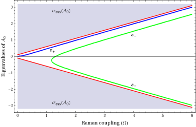
Figure 1. (Color online) Computed spectrum of operator $A_{0}$ (see Eq. (III.1) and Theorem III.2) for the point-interaction strength $\gamma=-1$ and the spin-orbit-coupling strength $\eta=0.6$ (in $\hbar=c=1$ units). The eigenvalues divided by $\eta>0$ are those of the one-dimensional Dirac-like operator for the particle of spin one-half and mass $\Omega/(2\eta)$ moving in the Fermi pseudopotential (III.7). In figure, red lines show the border of the essential spectrum of $A_{0}$, which is $\pm\Omega/2$. The blue $\varepsilon_{+}$ (green $\varepsilon_{-}$) line, showing the bound state as a function of the Raman coupling $\Omega>0$, corresponds to the eigenfunction with a zero-valued lower (upper) component at the origin $x=0$.

Remark III.3.

(1) In order to find the eigenvalues $\varepsilon\in\sigma_{\mathrm{disc}}(A_{0})$ explicitly, one needs to solve the cubic equation with respect to $\varepsilon$, as it is seen from Theorem III.2-(ii). The solutions to such type of equations are well known for a long time. However, their general form is rather complicated and we did not find it valuable here. Instead of that we displayed the spectrum of $A_{0}$ versus the Raman coupling $\Omega>0$ in Fig. 1.

(2) We also note that, unlike in Theorem III.2-(iii), where $f(0)$ is undetermined because of the delta-function, $f(0)$ in Theorem III.2-(ii) obeys the form as in (II.2a). The solutions in $\mathrm{ker}(\varepsilon\text{\large$\otimes$}I-A_{0})$ are strict so that $f(0)$ can be replaced by any constant ($1$, say).

Proof of Theorem III.2.

(i) The integral kernel $(A_{0}-z\text{\large$\otimes$}I)^{-1}(x)$ (for simplicity, we replace $x-x^{\prime}$ by $x$) is defined through the formal differential equation

$$(U+V_{F}\text{\large$\otimes$}I-z\text{\large$\otimes$}I)G_{0}(x;z)=\delta(x)\text{\large$\otimes$}I.$$

In agreement with (III.7), $G_{0}(x;z)$ is of the form

$$G_{0}(x;z)=\frac{1}{2\pi}\int_{-\infty}^{\infty}dp\>e^{ipx}\hat{G}_{0}(p;z),\quad\hat{G}_{0}(p;z)=\hat{G}_{0}^{0}(p;z)\Phi(\gamma;z),\quad\hat{G}_{0}^{0}(p;z)=\frac{z\text{\large$\otimes$}I+\hat{U}(p)}{\eta^{2}(p^{2}+\omega_{z}^{2})}$$ (III.8)

and $\Phi(\gamma;z)=I\text{\large$\otimes$}I-\gamma G_{0}(0;z)-G_{0}^{\prime}(0_{-};z)+G_{0}^{\prime}(0_{+};z)$. As one would have noticed, $\hat{G}_{0}^{0}(p;z)$ is the Fourier transform of $(A_{0}^{0}-z\text{\large$\otimes$}I)^{-1}(x)$. Recalling that the integrals $\int_{-\infty}^{\infty}dp\>e^{ipx}/(p^{2}+\omega^{2})=(\pi/\omega)e^{-\omega|x|}$, $\int_{-\infty}^{\infty}dp\>pe^{ipx}/(p^{2}+\omega^{2})=i\pi\>\mathrm{sgn}(x)e^{-\omega|x|}$ for $x\in\varmathbb{R}_{0}$ and $\mathrm{Re}\>\omega\neq 0$, we derive the expression

$$G_{0}(x;z)=(A_{0}^{0}-z\text{\large$\otimes$}I)^{-1}(x)\Phi(\gamma;z),$$ (III.9)

with the integral kernel $(A_{0}^{0}-z\text{\large$\otimes$}I)^{-1}(x)$ as in the theorem. By using this equation, calculate $G_{0}(0;z)=(G_{0}(0_{+};z)+G_{0}(0_{-};z))/2$ and $G_{0}^{\prime}(0_{\pm};z)$, and get the equation for $\Phi(\gamma;z)$,

$$[2\eta^{2}\omega_{z}\text{\large$\otimes$}I+(\gamma+2\omega_{z})((\Omega/2)\text{\large$\otimes$}\sigma_{3}+z\text{\large$\otimes$}I)]\Phi(\gamma;z)=2\eta^{2}\omega_{z}\text{\large$\otimes$}I.$$

Substitute obtained expression of $\Phi(\gamma;z)$ in (III.9), replace $x$ by $x-x^{\prime}$ back again and get (i), as required. Note that $f\in L^{1}(\varmathbb{R})^{2}$ is because of $(B_{0}-z\text{\large$\otimes$}I)R_{z}(A_{0})=I\text{\large$\otimes$}I$ (in the sense of distributions), that is, the resolvent of $A_{0}$ ($B_{0}$) is a distribution, and hence the equation $(A_{0}-z\text{\large$\otimes$}I)R_{z}(A_{0})=I\text{\large$\otimes$}I$ is meaningless in the classical sense.

(ii) The discrete spectrum is easily recovered by setting the denominator of the resolvent of $A_{0}$ equal to zero. As for the eigenfunctions, we begin with (III.2) by letting $z\equiv\varepsilon\in\sigma_{\mathrm{disc}}(A_{0})$ and $\omega_{\varepsilon}\equiv\omega$. We rewrite (III.2) in the following form

$$f_{1}(x)=\tfrac{1}{2}\Theta(x)e^{-\omega x}\left(c_{1}-c_{2}\sqrt{\frac{\Omega+2\varepsilon}{\Omega-2\varepsilon}}\right)+\tfrac{1}{2}\Theta(-x)e^{\omega x}\left(c_{1}+c_{2}\sqrt{\frac{\Omega+2\varepsilon}{\Omega-2\varepsilon}}\right),$$

$$f_{2}(x)=\tfrac{1}{2}\Theta(x)e^{-\omega x}\left(c_{2}-c_{1}\sqrt{\frac{\Omega-2\varepsilon}{\Omega+2\varepsilon}}\right)+\tfrac{1}{2}\Theta(-x)e^{\omega x}\left(c_{2}+c_{1}\sqrt{\frac{\Omega-2\varepsilon}{\Omega+2\varepsilon}}\right)$$ (III.10)

($|\varepsilon|<\Omega/2;\Omega,\eta>0;\omega>0$), where $f_{z\equiv\varepsilon}\equiv f$, and $f_{j,\varepsilon}\equiv f_{j}$ for $j=1,2$. By (III.10), with $f(0)$ as in (II.2a),

$$f(0)=\frac{1}{2}\left(\begin{matrix}c_{1}\\ c_{2}\end{matrix}\right),\quad f(0_{+})-f(0_{-})=-\left(\begin{matrix}c_{2}\sqrt{\frac{\Omega+2\varepsilon}{\Omega-2\varepsilon}}\\ c_{1}\sqrt{\frac{\Omega-2\varepsilon}{\Omega+2\varepsilon}}\end{matrix}\right),\quad f^{\prime}(0_{+})-f^{\prime}(0_{-})=-\omega\left(\begin{matrix}c_{1}\\ c_{2}\end{matrix}\right).$$

But $f\in D(A_{0})$, (III.1), and so it must hold

$$c_{1}\left(\frac{\gamma}{2}+\omega+\eta\sqrt{\frac{\Omega-2\varepsilon}{\Omega+2\varepsilon}}\right)=0,\quad c_{2}\left(\frac{\gamma}{2}+\omega-\eta\sqrt{\frac{\Omega+2\varepsilon}{\Omega-2\varepsilon}}\right)=0$$ (III.11)

($|\varepsilon|<\Omega/2;\Omega,\eta>0;\omega>0$), with $c_{j}=2f_{j}(0)$ for $j=1,2$. After some elementary simplifications, equations (III.10) and (III.11) lead to (ii).

(iii) Let $f\in\mathrm{ker}(\varepsilon\text{\large$\otimes$}I-B_{0})$ for some $\varepsilon\in\varmathbb{R}$. Combining the Fourier transform of (III.7) with (III.8) we get that

$$f(x)=-(A_{0}^{0}-\varepsilon\text{\large$\otimes$}I)^{-1}(x)\widehat{(V_{F}\text{\large$\otimes$}I)f},\quad\widehat{(V_{F}\text{\large$\otimes$}I)f}=\gamma f(0)+f^{\prime}(0_{-})-f^{\prime}(0_{+}).$$

Now, if we calculate $\gamma f(0)+f^{\prime}(0_{-})-f^{\prime}(0_{+})$ by taking $f$ from the left side of the above expressions, we get that $\widehat{(V_{F}\text{\large$\otimes$}I)f}=(\gamma+2\omega)f(0)$ and that

$$\left(I\text{\large$\otimes$}I+\frac{\gamma+2\omega}{2\eta^{2}\omega}\left((\Omega/2)\text{\large$\otimes$}\sigma_{3}+\varepsilon\text{\large$\otimes$}I\right)\right)f(0)=0\quad(\eta>0;\omega>0)$$

thus yielding (iii).

(iv) The essential spectrum of $A_{0}$ is found from the dispersion curve $\varepsilon(p)$ which in turn is found by taking the Fourier transform of $U$ and solving the eigenvalue equation, namely,

$$\det\left(\begin{matrix}\Omega/2-\varepsilon(p)&-i\eta p\\ i\eta p&-\Omega/2-\varepsilon(p)\end{matrix}\right)=0.$$

The result reads $\varepsilon(p)=\pm\sqrt{(\Omega/2)^{2}+(\eta p)^{2}}$ for all $p\in\varmathbb{R}$.

The essential spectrum of $B_{0}$ is found from the integral kernel of the resolvent of $A_{0}$, by virtue of (iii). This is exactly the case as for deriving the spectrum of $A_{0}^{0}$. Then one needs to solve $p^{2}+\omega_{z}^{2}=0$ with respect to $z\equiv\varepsilon(p)$ ($p\in\varmathbb{R}$). The solutions are those as above, and hence (iv) holds.

(v) The present item immediately follows from (iv) and from the requirement that, for $\varepsilon\in\sigma_{\mathrm{disc}}(A_{0})$, it holds $-\Omega/2<\varepsilon<\Omega/2$. ∎

IV. Spin-orbit coupling induced states

Lemma IV.1.

We have:

1. $[A,A_{0}]=0$ on $D(A)$ strictly;

2. $[B,B_{0}]=0$ almost everywhere in $\varmathbb{R}\text{\large$\otimes$}\varmathbb{C}^{2}$.

Proof.

We note that $W^{p}(\varmathbb{R}_{0})^{2}\subset W^{p^{\prime}}(\varmathbb{R}_{0})^{2}$ for $p>p^{\prime}$; see eg (Herczyński, 1989, p. 276). By (II.5) and (III.1), $D(A)\subset D(A_{0})$. By (II.6) and (III.7), $D(B)\subset D(B_{0})$. Thus $[A,A_{0}]$ makes sense since $R(A_{0})\cap D(A)\subset R(A_{0})\cap D(A_{0})=D(A_{0})$, $R(A)\cap D(A_{0})\supset D(A)\cap D(A_{0})=D(A)$, and the same for $[B,B_{0}]$ ($R$ is the range).

Item (1) is easy to perform: $[A,A_{0}]$ on $D(A)$ is given by $[H_{0},U]=[-\Delta\text{\large$\otimes$}I,U]=0$. The same applies to the resolvents $R_{z_{0}}(A_{0})$, $R_{z}(A)$ ($z_{0},z\in\varmathbb{C}$) and to the exponents $e^{itA_{0}}$, $e^{isA}$ ($t,s\in\varmathbb{R}$) in consonance with (Reed and Simon, 1980, Theorem VIII.13). The fact that the exponents commute follows from the commutation relation of resolvents. This can be seen by noting eg $R_{z_{0}}(A_{0})=i\int_{0}^{\infty}dt\>e^{-it(B_{0}-z_{0}\otimes I)}$ ($\mathrm{Im}\>z_{0}>0$). That the resolvents commute (weakly), the easiest way to see this is to apply (III.8) and (IV.2), where one concludes that the integral $\int_{-\infty}^{\infty}([R_{z}(A),R_{z_{0}}(A_{0})]f)(x)dx$ is equal to $\int_{-\infty}^{\infty}[\hat{G}(0;z),\hat{G}_{0}(0;z_{0})]f(x)dx=0$, provided $f\in L^{1}(\varmathbb{R})^{2}$.

In order to prove (2), we integrate $[B,B_{0}]$ in the interval $X\subseteq\varmathbb{R}_{0}$ because $D(B)\subset D(B_{0})$ contains functions which are well-defined for $x\in\varmathbb{R}_{0}$. In this case, all integrands containing $\delta$ or $\delta^{\prime}$ (see (III.6)) vanish because the argument of $\delta$ ($\delta^{\prime}$) is nonzero for all $x\in X$. The remaining terms, that is, those which do not include deltas, commute with each other. Finally, we extend $X\subseteq\varmathbb{R}_{0}$ to the whole $\varmathbb{R}$ by setting $X=(-\infty,-\epsilon)\cup(\epsilon,\infty)$ as $\epsilon\downarrow 0$, and we have (2). ∎

We already know from Theorem III.2-(ii) that $\mathrm{ker}(\varepsilon\text{\large$\otimes$}I-A_{0})\subset D(A_{0})$ is a nonempty set for $\varepsilon\in\sigma_{\mathrm{disc}}(A_{0})$. Now, we assume that $\sigma_{\mathrm{disc}}(A)\neq\varnothing$, and let $\lambda\in\sigma_{\mathrm{disc}}(A)$. Then by Lemma IV.1,

$$D(A)\supset\mathrm{ker}(\varepsilon\text{\large$\otimes$}I-A_{0})\cap\mathrm{ker}(\lambda\text{\large$\otimes$}I-A)\equiv\mathrm{ker}(\lambda(\varepsilon)\text{\large$\otimes$}I-A)$$ (IV.1)

for some $\lambda(\varepsilon)\in\sigma_{\mathrm{so}}(A)\subset\sigma_{\mathrm{disc}}(A)$. We say that the set $\sigma_{\mathrm{so}}(A)$ contains spin-orbit coupling induced states $\lambda(\varepsilon)$. This is because $\sigma_{\mathrm{so}}(A)$ is nonempty only for nonzero spin-orbit coupling $\eta>0$, in agreement with Theorem III.2.

Here, our main goal is to establish $\sigma_{\mathrm{so}}(A)$. For that reason we prove that:

Lemma IV.2.

Let $A$ and $B$ be as in (II.5) and (II.6). Then:

1. The resolvent of $A$ is given by

   $$(R_{z}(A)f)(x)= \int_{-\infty}^{\infty}dx^{\prime}\>(A-z\text{\large$\otimes$}I)^{-1}(x-x^{\prime})f(x^{\prime})$$

   ($$f\in L^{2}(\varmathbb{R})^{2}\cap L^{1}(\varmathbb{R})^{2}$$), with the integral kernel (Green’s function)

   $$(A-z\text{\large$\otimes$}I)^{-1}(x-x^{\prime})= 2p_{1}p_{2}(p_{1}+p_{2})(A^{0}-z\text{\large$\otimes$}I)^{-1}(x-x^{\prime})$$

   $$\times\frac{p_{1}p_{2}(i\gamma+2(p_{1}+p_{2}))\text{\large$\otimes$}I-i\gamma((\Omega/2)\text{\large$\otimes$}\sigma_{3}-z\text{\large$\otimes$}I)}{(2p_{1}p_{2}(p_{1}+p_{2})+i\gamma(p_{1}p_{2}+z))^{2}+(\gamma\Omega/2)^{2}}$$

   ($$x\neq x^{\prime};x,x^{\prime}\in\varmathbb{R};z\in\varmathbb{C}\backslash\sigma(A);\Omega,\eta\geq 0;\gamma\in\varmathbb{R};\mathrm{Im}\>p_{j}>0;j=1,2 A^{0}=H_{0}\upharpoonright W_{0}^{2}(\varmathbb{R}_{0})^{2} A^{0}$$), where , and the integral kernel of is given by

   $$(A^{0}-z\text{\large$\otimes$}I)^{-1}(x-x^{\prime})= \frac{i}{2(p_{1}^{2}-p_{2}^{2})}\Biggl{(}\frac{e^{ip_{1}(x-x^{\prime})}}{p_{1}}(p_{1}^{2}\text{\large$\otimes$}I-z\text{\large$\otimes$}I-\hat{U}(p_{1}))$$

   $$-\frac{e^{ip_{2}(x-x^{\prime})}}{p_{2}}(p_{2}^{2}\text{\large$\otimes$}I-z\text{\large$\otimes$}I-\hat{U}(p_{2}))\Biggr{)}\quad(x>x^{\prime}),$$

   $$= \frac{i}{2(p_{1}^{2}-p_{2}^{2})}\Biggl{(}\frac{e^{-ip_{1}(x-x^{\prime})}}{p_{1}}(p_{1}^{2}\text{\large$\otimes$}I-z\text{\large$\otimes$}I-\hat{U}(-p_{1}))$$

   $$-\frac{e^{-ip_{2}(x-x^{\prime})}}{p_{2}}(p_{2}^{2}\text{\large$\otimes$}I-z\text{\large$\otimes$}I-\hat{U}(-p_{2}))\Biggr{)}\quad(x<x^{\prime})$$

   ($x,x^{\prime}\in\varmathbb{R};z\in\varmathbb{C}\backslash\sigma(A^{0});\Omega,\eta\geq 0;\mathrm{Im}\>p_{j}>0;j=1,2$), $p_{1,2}=s_{1,2}\sqrt{z+\eta^{2}/2\pm(1/2)\sqrt{\eta^{2}(\eta^{2}+4z)+\Omega^{2}}}$ ($s_{j}=\pm 1;j=1,2$);

2. $\sigma_{\mathrm{ess}}(A)=\sigma_{\mathrm{ess}}(B)=\sigma(A^{0})=[J(\eta,\Omega),\infty)$, where $J(\eta,\Omega)$ is equal to $\lambda_{0}\equiv-[\eta^{2}+(\Omega/\eta)^{2}]/4$ for $0\leq\Omega\leq\eta^{2}$, and to $-\Omega/2$ for $\Omega>\eta^{2}\geq 0$.

Proof.

(i) The proof is pretty much similar to that of (II.8) and Theorem III.2-(i). The integral kernel $(A-z\text{\large$\otimes$}I)^{-1}(x)$ (for simplicity, we replace $x-x^{\prime}$ by $x$) is defined through the formal differential equation

$$(-\Delta\text{\large$\otimes$}I+U+\gamma\delta(x)\text{\large$\otimes$}I-z\text{\large$\otimes$}I)G(x;z)=\delta(x)\text{\large$\otimes$}I.$$

Then

$$G(x;z)=\frac{1}{2\pi}\int_{-\infty}^{\infty}dp\>e^{ipx}\hat{G}(p;z),\quad\hat{G}(p;z)=\hat{G}^{0}(p;z)\Psi(\gamma;z),\quad\hat{G}^{0}(p;z)=\frac{(p^{2}-z)\text{\large$\otimes$}I-\hat{U}(p)}{\Delta_{z}(p)},$$ (IV.2)

with $\Delta_{z}(p)$ as in (II.8) and $\Psi(\gamma;z)=I\text{\large$\otimes$}I-\gamma G(0;z)$. As one would have noticed, $\hat{G}^{0}(p;z)$ is the Fourier transform of $(A^{0}-z\text{\large$\otimes$}I)^{-1}(x)$. For more convenience, we rewrite the denominator by $\Delta_{z}(p)=(p^{2}-p_{1}^{2})(p^{2}-p_{2}^{2})$, with $p_{j}$ ($j=1,2$) as in Lemma IV.2-(i).

Without loss of generality, we assume that $\mathrm{Im}\>p_{j}>0$ ($j=1,2$). Then the integration over $p\in\varmathbb{R}$ can be performed in two distinct ways. Consider

$$\varphi(\zeta)=\frac{e^{i\zeta x}((\zeta^{2}-z)\text{\large$\otimes$}I-\eta\zeta\text{\large$\otimes$}\sigma_{2}-(\Omega/2)\text{\large$\otimes$}\sigma_{3})}{(\zeta^{2}-p_{1}^{2})(\zeta^{2}-p_{2}^{2})}\quad(x\in\varmathbb{R}_{0};z,\zeta\in\varmathbb{C}),$$

and integrate it around the contour $\mathcal{C}$ oriented counterclockwise, with the poles $p_{1}$, $p_{2}$. This implies that the integral exists for $x>0$. Similarly, integrate $\varphi(\zeta)$ around the contour $\mathcal{C}^{\prime}$ oriented counterclockwise but with the poles $-p_{1}$, $-p_{2}$, and get $x<0$ for the existence of the integral. [We note that these two contours of integration are not unique. One can choose, for example, the contour with poles $p_{1}$, $-p_{2}$ ($\mathrm{Im}\>p_{1}>0;\mathrm{Im}\>p_{2}<0$) so that the integral exists for $x>0$, and the contour with poles $-p_{1}$, $p_{2}$ (again, $\mathrm{Im}\>p_{1}>0;\mathrm{Im}\>p_{2}<0$) so that the integral exists for $x<0$.]

By the residue theorem,

$$\int_{-\infty}^{\infty}\varphi(p)dp+\lim_{R\to\infty}\int_{\mathcal{C}}\varphi(\zeta)d\zeta=2\pi i\underset{\zeta=p_{1},p_{2}}{\mathrm{res}}\>\varphi(\zeta),$$

$$-\int_{-\infty}^{\infty}\varphi(p)dp+\lim_{R\to\infty}\int_{\mathcal{C}^{\prime}}\varphi(\zeta)d\zeta=2\pi i\underset{\zeta=-p_{1},-p_{2}}{\mathrm{res}}\>\varphi(\zeta),$$

where the contour integration is performed over $\zeta=Re^{i\psi}$ ($\psi\in[0,\pi]$) in the first contour, and over $\zeta=Re^{i\psi}$ ($\psi\in[\pi,2\pi]$) in the second contour. In the limit $R\to\infty$, function $|\varphi(\zeta)|\to 0$ for $x>0$ in the first integral, and for $x<0$ in the second one.

The residues are easy to calculate by noting that

$$\frac{1}{(z^{2}-p_{1}^{2})(z^{2}-p_{2}^{2})}=\frac{1}{2(p_{1}^{2}-p_{2}^{2})}\left(\frac{1}{p_{1}(z-p_{1})}-\frac{1}{p_{1}(z+p_{1})}-\frac{1}{p_{2}(z-p_{2})}+\frac{1}{p_{2}(z+p_{2})}\right).$$

After some elementary simplifications, and replacing $x$ with $x-x^{\prime}$, we obtain the integral kernel of the resolvent of $A^{0}$ as in Lemma IV.2-(i).

Following (IV.2),

$$G(x;z)=(A^{0}-z\text{\large$\otimes$}I)^{-1}(x)\Psi(\gamma;z).$$ (IV.3)

By using this equation, calculate $G(0;z)=(G(0_{+};z)+G(0_{-};z))/2$ and get the equation for $\Psi(\gamma;z)$,

$$[(i\gamma+2(p_{1}+p_{2}))\text{\large$\otimes$}I+(i\gamma/(p_{1}p_{2}))((\Omega/2)\text{\large$\otimes$}\sigma_{3}+z\text{\large$\otimes$}I)]\Psi(\gamma;z)=2(p_{1}+p_{2})\text{\large$\otimes$}I.$$

Substitute obtained expression of $\Psi(\gamma;z)$ in (IV.3), replace $x$ with $x-x^{\prime}$ and get the resolvent of $A$ as required. That $f\in L^{1}(\varmathbb{R})^{2}$, the arguments are those as in the proof of Theorem III.2-(i).

Figure 2. (Color online) Computed lower branch of dispersion in (IV.4) for the spin-orbit-coupling strength $\eta=0.6$ (in $\hbar=c=1$ units), for a range of Raman couplings $\Omega\geq 0$. As $\Omega$ increases ($\Omega>\eta^{2}$), the two dressed spin states (Lin et al., 2011) are merged into a single minimum $-\Omega/2$ at $p=0$. This is a regime when the spin-orbit coupling induced states $\sigma_{\mathrm{so}}(A)$, Theorem IV.4, are observed below the continuous spectrum as well as above it. For $\Omega\leq\eta^{2}$, the spin states have two minima $-[\eta^{2}+(\Omega/\eta)^{2}]/4$ at $p=\pm\sqrt{\eta^{4}-\Omega^{2}}/(2\eta)$, and the spin-orbit induced states are embedded into the essential spectrum of $A$.

(ii) The essential spectrum of $A$ as well as the spectrum of $A^{0}$ is found from (IV.2) by solving $\Delta_{z}(p)=0$ ($p\in\varmathbb{R}$) with respect to $z\equiv\lambda(p)$, whereas for $B$, one needs to solve the same equation due to (II.8). The solutions read

$$\lambda_{\pm}(p)=p^{2}\pm\sqrt{\eta^{2}p^{2}+(\Omega/2)^{2}}\geq\lambda_{-}(p).$$ (IV.4)

The lower bound of $\lambda_{\pm}(p)$ is found by differentiating $\lambda_{-}(p)$ with respect to $p\in\varmathbb{R}$. One finds three critical points: $p_{1}=0$, $p_{2}=-\sqrt{\eta^{4}-\Omega^{2}}/(2\eta)$ and $p_{3}=\sqrt{\eta^{4}-\Omega^{2}}/(2\eta)$. As seen, $p_{2}$ and $p_{3}$ are in $\varmathbb{R}$ only for $\Omega\leq\eta^{2}$. Hence it holds $\lambda_{\pm}(p)\geq-[\eta^{2}+(\Omega/\eta)^{2}]/4$. If, however, $\Omega>\eta^{2}$, only $p_{1}$ is valid. Then $\lambda_{\pm}(p)\geq-\Omega/2$. This proves that $\sigma_{\mathrm{ess}}(A)=\sigma_{\mathrm{ess}}(B)$, hence (ii), and the proof of the statement is accomplished. ∎

Remark IV.3.

For the illustrative and comparison purposes (see (Lin et al., 2011, Fig. 1b) and (Galitski and Spielman, 2013, Fig. 2c)), we displayed the dispersion relation $\lambda_{-}(p)$, (IV.4), in Fig. 2.

We are now in a position to establish the properties of spin-orbit coupling induced states.

Theorem IV.4.

Given $A$ as in (II.5) and $A_{0}$ as in (III.1). Then:

1. $\sigma_{\mathrm{disc}}(A)\supset\sigma_{\mathrm{so}}(A)=\bigl{\{}\varepsilon-\omega^{2}\!\colon\thinspace\varepsilon\in\sigma_{\mathrm{disc}}(A_{0})\backslash\bigl{\{}-\eta^{2}/2,\Omega/2-\eta^{2}\bigr{\}};\Omega,\eta>0\bigr{\}}$;

2. $\sigma_{\mathrm{so}}(A)=\sigma_{<}(A)\cup\sigma_{>}(A),\quad\sigma_{>}(A)=\sigma_{1}(A)\cup\sigma_{2}(A)$;

3. $\sigma_{<}(A)=\bigl{\{}\lambda(\varepsilon)\in\sigma_{\mathrm{so}}(A)\!\colon\thinspace\varepsilon\in\sigma_{\mathrm{disc}}(A_{0});-\Omega/2<\varepsilon<\Omega/2-\eta^{2};\Omega>\eta^{2}>0\bigr{\}}$;

4. $\sigma_{1}(A)=\bigl{\{}\lambda(\varepsilon)\in\sigma_{\mathrm{so}}(A)\!\colon\thinspace\varepsilon\in\sigma_{\mathrm{disc}}(A_{0});\Omega/2-\eta^{2}<\varepsilon<\Omega/2;\Omega>\eta^{2}>0\bigr{\}}$;

5. $\sigma_{2}(A)=\bigl{\{}\lambda(\varepsilon)\in\sigma_{\mathrm{so}}(A)\!\colon\thinspace\varepsilon\in\sigma_{\mathrm{disc}}(A_{0});0<\Omega\leq\eta^{2}\bigr{\}}$;

6. $\sigma_{\mathrm{so}}(A)\cap\sigma_{\mathrm{ess}}(A)=\sigma_{2}(A)$ for $0<\Omega\leq\eta^{2}$;

7. $\sigma_{\mathrm{so}}(A)\cap\sigma_{\mathrm{ess}}(A)=\sigma_{1}(A)$ for $\Omega>\eta^{2}>0$;

8. $\sigma_{\mathrm{so}}(B)=\sigma_{\mathrm{so}}(A)$. The equivalence classes of functions from the kernel $\mathrm{ker}(\lambda(\varepsilon)\text{\large$\otimes$}I-B)$, for $\lambda(\varepsilon)\in\sigma_{\mathrm{so}}(B)$, are of the form given in Theorem III.2-(iii).

The eigenfunctions that correspond to $\lambda(\varepsilon)\in\sigma_{\mathrm{so}}(A)$ are as in Theorem III.2-(ii).

Proof.

The proof is essentially based on the combination of Theorem III.2 with Lemmas IV.1–IV.2.

(i) In agreement with Lemma IV.1-(1), and in particular (IV.1), substitute $f\in\mathrm{ker}(\varepsilon\text{\large$\otimes$}I-A_{0})$ (refer to Theorem III.2-(ii)) in $\mathrm{ker}(\lambda(\varepsilon)\text{\large$\otimes$}I-A)$ for some $\lambda(\varepsilon)\in\varmathbb{R}$. Then

$$0= f_{1}(0)\left(-\omega^{2}+\frac{\Omega}{2}-\lambda(\varepsilon)-\omega\eta\sqrt{\frac{\Omega-2\varepsilon}{\Omega+2\varepsilon}}\right)$$

$$+f_{2}(0)\left(\mp\left(-\omega^{2}+\frac{\Omega}{2}-\lambda(\varepsilon)\right)\sqrt{\frac{\Omega+2\varepsilon}{\Omega-2\varepsilon}}\pm\omega\eta\right),$$

$$0= f_{1}(0)\left(\mp\left(-\omega^{2}-\frac{\Omega}{2}-\lambda(\varepsilon)\right)\sqrt{\frac{\Omega-2\varepsilon}{\Omega+2\varepsilon}}\mp\omega\eta\right)$$

$$+f_{2}(0)\left(-\omega^{2}-\frac{\Omega}{2}-\lambda(\varepsilon)+\omega\eta\sqrt{\frac{\Omega+2\varepsilon}{\Omega-2\varepsilon}}\right)$$

($\omega$ as in Theorem III.2), where the upper sign corresponds to $x>0$, and the lower one to $x<0$. It appears from above that for either $f_{2}(0)=0$ or $f_{1}(0)=0$, the following holds,

$$0= -\omega^{2}+\frac{\Omega}{2}-\lambda(\varepsilon)-\omega\eta\sqrt{\frac{\Omega-2\varepsilon}{\Omega+2\varepsilon}},$$

$$0= -\omega^{2}-\frac{\Omega}{2}-\lambda(\varepsilon)+\omega\eta\sqrt{\frac{\Omega+2\varepsilon}{\Omega+2\varepsilon}}.$$

The solution $\lambda(\varepsilon)$ satisfying the above system of equations is given by $\lambda(\varepsilon)=\varepsilon-\omega^{2}$ or explicitly, $\varepsilon-(\Omega^{2}-4\varepsilon^{2})/(4\eta^{2})$.

In order to accomplish the proof of (i), it remains to establish valid eigenvalues $\varepsilon$ from $\sigma_{\mathrm{disc}}(A_{0})$ thus generating proper eigenvalues $\lambda(\varepsilon)$ from $\sigma_{\mathrm{so}}(A)$.

By a straightforward inspection, $\lambda_{0}\leq\lambda(\varepsilon)<\Omega/2$ for all $\Omega,\eta>0$, where $\lambda_{0}$ is as in Lemma IV.2-(ii). The lower bound is obtained at $\varepsilon=-\eta^{2}/2$ (the solution to $d\lambda(\varepsilon)/d\varepsilon=0$). On the other hand, $\lambda_{0}\leq-\Omega/2$ and $\lambda(\varepsilon)=-\Omega/2$ at $\varepsilon=\Omega/2-\eta^{2}$ ($\varepsilon=-\Omega/2$ is improper due to Theorem III.2-(ii)). Therefore, the points $\varepsilon=-\eta^{2}/2$ and $\Omega/2-\eta^{2}$, which hold whenever $\Omega>\eta^{2}>0$, must be excluded as the resonant states, by Theorem III.2-(i) (inspect solutions to $\omega_{z}=0$ with respect to $z$ given by $\pm\Omega/2$) and by Lemma IV.2-(i) (inspect solutions to $p_{1}^{2}=p_{2}^{2}$ with respect to $z$ given by $\lambda_{0}$, and solutions to $p_{j}=0$, $j=1,2$, given by $\pm\Omega/2$). Item (i) holds.

(ii)–(v) The reason for extracting $\sigma_{\mathrm{so}}(A)$ into subsets is in different behavior of the involved eigenvalues: $\sup\sigma_{<}(A)=\inf\sigma_{\mathrm{ess}}(A)$ and $\inf\sigma_{>}(A)=\inf\sigma_{\mathrm{ess}}(A)$. This is easy to verify by considering $\lambda(\varepsilon)$ and $J(\eta,\Omega)$: For $0<\Omega\leq\eta^{2}$, one finds that $\lambda(\varepsilon)>J(\eta,\Omega)$, which is $\sigma_{2}(A)$. For $\Omega>\eta^{2}>0$, $\lambda(\varepsilon)<J(\eta,\Omega)$ for $-\Omega/2<\varepsilon<\Omega/2-\eta^{2}$, thus yielding $\sigma_{<}(A)$, and $\lambda(\varepsilon)>J(\eta,\Omega)$ for $\Omega/2-\eta^{2}<\varepsilon<\Omega/2$, thus yielding $\sigma_{1}(A)$. The values $\lambda(\varepsilon)=J(\eta,\Omega)$ are excluded due to the previous discussion (these are resonant states).

(vi) Since $J(\eta,\Omega)=\lambda_{0}$ for $0<\Omega\leq\eta^{2}$, we have that $\sigma_{\mathrm{so}}(A)=\sigma_{2}(A)$ in this regime. But $\inf\sigma_{2}(A)=\inf\sigma_{\mathrm{ess}}(A)$, and hence (vi) holds.

(vii) For $\Omega>\eta^{2}>0$, $J(\eta,\Omega)=-\Omega/2$. In the present regime we have that $\sigma_{\mathrm{so}}(A)=\sigma_{1}(A)$ with $\inf\sigma_{1}(A)=-\Omega/2$. This gives (vii).

(viii) Following Lemma IV.1-(2), we need to show that (weak) solutions in $\mathrm{ker}(\lambda(\varepsilon)\text{\large$\otimes$}I-B)$ yield eigenvalues $\lambda(\varepsilon)\in\sigma_{\mathrm{so}}(B)=\sigma_{\mathrm{so}}(A)$. By Theorem III.2-(iii),

$$0=\int_{-\infty}^{\infty}(B-\lambda(\varepsilon)\text{\large$\otimes$}I)f(x)dx=\int_{-\infty}^{\infty}(H_{0}f)(x)dx+(\gamma-2\lambda(\varepsilon)/\omega)f(0),$$ (IV.5a)

where we have explored the integral $\int_{-\infty}^{\infty}f(x)dx=(2/\omega)f(0)$ for $\omega>0$ (recall $f\in L^{1}(\varmathbb{R})^{2}$ in Theorem III.2-(i) and Lemma IV.2-(i)). But

$$\int_{-\infty}^{\infty}(H_{0}f)(x)dx= -\int_{-\infty}^{\infty}f^{\prime\prime}(x)dx-(i\eta\text{\large$\otimes$}\sigma_{2})\int_{-\infty}^{\infty}f^{\prime}(x)dx$$

$$+((\Omega/2)\text{\large$\otimes$}\sigma_{3})\int_{-\infty}^{\infty}f(x)dx=((\Omega/\omega)\text{\large$\otimes$}\sigma_{3})f(0),$$ (IV.5b)

and hence the combination of (IV.5) yields

$$((\Omega/2)\text{\large$\otimes$}\sigma_{3}+(\gamma\omega/2-\lambda(\varepsilon))\text{\large$\otimes$}I)f(0)=0.$$ (IV.6)

Equation (IV.6) has solutions with respect to $\lambda(\varepsilon)\in\varmathbb{R}$ only if either $f_{2}(0)=0$ or $f_{1}(0)=0$ (recall Theorem III.2). Then it holds $\lambda(\varepsilon)=(\gamma\omega\pm\Omega)/2$, where the upper sign is for $f_{2}(0)=0$, and the lower one for $f_{1}(0)=0$. Recalling that $\omega=\sqrt{(\Omega/2)^{2}-\varepsilon^{2}}/\eta$, we recover $\sigma_{\mathrm{so}}(A)$. This accomplishes the proof of the theorem. ∎

The points in $\sigma_{\mathrm{so}}(A)\subset\sigma_{\mathrm{disc}}(A)$ are illustrated in Fig. 3.

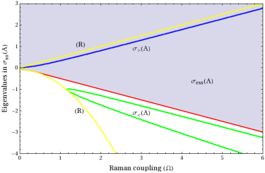
Figure 3. (Color online) Computed spin-orbit coupling induced states $\sigma_{\mathrm{so}}(A)\subset\sigma_{\mathrm{disc}}(A)$ (refer to Theorem IV.4) for the point-interaction strength $\gamma=-1$ and the spin-orbit-coupling strength $\eta=0.6$ (in $\hbar=c=1$ units). In figure, red line shows the border $\inf\sigma_{\mathrm{ess}}(A)$ of the essential spectrum of $A$ (Lemma IV.2). The eigenvalues $\lambda(\varepsilon)\in\sigma_{\mathrm{so}}(A)$ ($\varepsilon\in\sigma_{\mathrm{disc}}(A_{0})$), as functions of the Raman coupling $\Omega>0$, are drawn by the blue ($\sigma_{>}(A)$) and green ($\sigma_{<}(A)$) lines. Resonant states of $A$ are drawn by yellow curves (R).

V. Discrete spectrum

As yet, we have established the part of $\sigma_{\mathrm{disc}}(A)$ which is associated with discontinuous eigenfunctions at $x=0$. These states originate from the property that $A$ commutes with $A_{0}$, where $A_{0}/\eta$ ($\eta>0$) is unitarily equivalent to the one-dimensional Dirac operator for the particle in Fermi pseudopotential.

In this section, our main goal is to determine the remaining part of $\sigma_{\mathrm{disc}}(A)$, namely, $\sigma_{\mathrm{disc}}(A)\backslash\sigma_{\mathrm{so}}(A)$, thus recovering all discrete states of the spin-orbit Hamiltonian, and to show that the associated eigenfunctions are continuous in the whole $\varmathbb{R}$.

Theorem V.1.

Let $A$ and $B$ be as in (II.5) and (II.6), respectively. Then:

1. $$\sigma_{\mathrm{disc}}(A)= \sigma_{\mathrm{disc}}(B)=\bigl{\{}\lambda<-\Omega/2\!\colon\thinspace 2p_{1}p_{2}(p_{1}+p_{2})+i\gamma(p_{1}p_{2}+\lambda\pm\Omega/2)=0;$$

   $$\lambda\neq\lambda_{0};\Omega\geq 0;\eta>0;\gamma<0;\mathrm{Im}\>p_{j}>0;j=1,2\bigr{\}}\bigcup\sigma_{\mathrm{so}}(A),$$

   where $\sigma_{\mathrm{so}}(A)$ is given in Theorem IV.4, the $p_{j}$ ($j=1,2$) and $\lambda_{0}$ are as in Lemma IV.2, with $s_{1}=+1$, $s_{2}=\pm 1$, $z\equiv\lambda$;

2. The equivalence classes of functions from $\mathrm{ker}(\lambda\text{\large$\otimes$}I-B)$ (with $\lambda\in\sigma_{\mathrm{disc}}(B)\backslash\sigma_{\mathrm{so}}(B)$) are of the form $-\gamma(A^{0}-\lambda\text{\large$\otimes$}I)^{-1}(x)f(0)$ (with $x\in\varmathbb{R}_{0};\gamma<0$), with the integral kernel, for $z\equiv\lambda$, as in Lemma IV.2-(i);

3. The (strict) solutions $\mathrm{ker}(\lambda\text{\large$\otimes$}I-A)$ associated with $\lambda$ from $\sigma_{\mathrm{disc}}(A)\backslash\sigma_{\mathrm{so}}(A)$ are of the form:

   1. For $\lambda\in\sigma_{\mathrm{disc}}(A)\backslash\sigma_{\mathrm{so}}(A)$ with the upper sign,

      $$f(x)= C\left[\frac{e^{ip_{1}x}}{p_{1}}\left(\begin{matrix}\lambda+\Omega/2-p_{1}^{2}\\ i\eta p_{1}\end{matrix}\right)-\frac{e^{ip_{2}x}}{p_{2}}\left(\begin{matrix}\lambda+\Omega/2-p_{2}^{2}\\ i\eta p_{2}\end{matrix}\right)\right]\quad(x>0),$$ (V.1a)

      $$= C\left[\frac{e^{-ip_{1}x}}{p_{1}}\left(\begin{matrix}\lambda+\Omega/2-p_{1}^{2}\\ -i\eta p_{1}\end{matrix}\right)-\frac{e^{-ip_{2}x}}{p_{2}}\left(\begin{matrix}\lambda+\Omega/2-p_{2}^{2}\\ -i\eta p_{2}\end{matrix}\right)\right]\quad(x<0)$$ (V.1b)

      for any $C\in\varmathbb{C}\backslash\{0\}$, $\eta>0$;

   2. For $\lambda\in\sigma_{\mathrm{disc}}(A)\backslash\sigma_{\mathrm{so}}(A)$ with the lower sign,

      $$f(x)= C\left[\frac{e^{ip_{1}x}}{\lambda+\Omega/2-p_{1}^{2}}\left(\begin{matrix}\lambda+\Omega/2-p_{1}^{2}\\ i\eta p_{1}\end{matrix}\right)-\frac{e^{ip_{2}x}}{\lambda+\Omega/2-p_{2}^{2}}\left(\begin{matrix}\lambda+\Omega/2-p_{2}^{2}\\ i\eta p_{2}\end{matrix}\right)\right]$$

      $$(x>0),$$ (V.2a)

      $$= C\left[-\frac{e^{-ip_{1}x}}{\lambda+\Omega/2-p_{1}^{2}}\left(\begin{matrix}\lambda+\Omega/2-p_{1}^{2}\\ -i\eta p_{1}\end{matrix}\right)+\frac{e^{-ip_{2}x}}{\lambda+\Omega/2-p_{2}^{2}}\left(\begin{matrix}\lambda+\Omega/2-p_{2}^{2}\\ -i\eta p_{2}\end{matrix}\right)\right]$$

      $$(x<0)$$ (V.2b)

      for any $C\in\varmathbb{C}\backslash\{0\}$, $\eta>0$;

   3. For $\eta=0$, we have that the discrete spectrum is given by the union $\sigma_{\mathrm{disc}}(A)\backslash\sigma_{\mathrm{so}}(A)=\sigma_{\mathrm{disc}}(A)=\bigl{\{}-\gamma^{2}/4\pm\Omega/2\!\colon\thinspace\gamma<-2\sqrt{\Omega}\bigr{\}}\cup\bigl{\{}-\gamma^{2}/4-\Omega/2\!\colon\thinspace-2\sqrt{\Omega}<\gamma<0\bigr{\}}$; the associated eigenfunctions are $C\chi_{\pm}e^{\gamma|x|/2}$, with $\sigma_{3}\chi_{\pm}=\pm\chi_{\pm}$ ($x\in\varmathbb{R}_{0};C\in\varmathbb{C}\backslash\{0\};\Omega\geq 0;\gamma<0$);

4. There are no eigenvalues from $\sigma_{\mathrm{disc}}(A)\backslash\sigma_{\mathrm{so}}(A)$ embedded into the essential spectrum of $A$: $(\sigma_{\mathrm{disc}}(A)\backslash\sigma_{\mathrm{so}}(A))\cap\sigma_{\mathrm{ess}}(A)=\varnothing$.

Remark V.2.

(1) As is seen from the theorem, the eigenfunctions of $A$ and $B$, which correspond to the upper sign for $\lambda$ in $\sigma_{\mathrm{disc}}(A)\backslash\sigma_{\mathrm{so}}(A)$, coincide if and only if

$$f_{1}(0)\equiv f_{1}(0_{+})=f_{1}(0_{-})=\frac{-2iC}{\gamma}(p_{1}^{2}-p_{2}^{2}),\quad f_{2}(0)\equiv f_{2}(0_{+})=f_{2}(0_{-})=0$$ (V.3a)

($C\in\varmathbb{C}\backslash\{0\};\gamma<0$). The eigenfunctions of $A$ and $B$, which correspond to the lower sign for $\lambda$ in $\sigma_{\mathrm{disc}}(A)\backslash\sigma_{\mathrm{so}}(A)$, coincide if and only if

$$f_{1}(0)\equiv f_{1}(0_{+})=f_{1}(0_{-})=0,\quad f_{2}(0)\equiv f_{2}(0_{+})=f_{2}(0_{-})=\frac{2C}{\gamma\eta}(p_{1}^{2}-p_{2}^{2})$$ (V.3b)

($C\in\varmathbb{C}\backslash\{0\};\gamma<0;\eta>0$).

Therefore, equations (V.3) provide unique solutions (up to the constant $C$) for functions $f_{j}(0)$ ($j=1,2$) which are undetermined in $\mathrm{ker}(\lambda\text{\large$\otimes$}I-B)$; see Theorem V.1-(2).

(2) It is interesting to compare the eigenfunctions at $x=0$ (having the meaning as in (II.2a)), which correspond to the spin-orbit coupling induced states (Theorem IV.4), with those given above. For $\lambda(\varepsilon)\in\sigma_{\mathrm{so}}(A)$ with the upper sign, $f_{2}(0_{+})=-f_{2}(0_{-})$ yields $f_{2}(0)=0$; in comparison, $f_{2}(0)\equiv f_{2}(0_{+})=f_{2}(0_{-})=0$ for $\lambda\in\sigma_{\mathrm{disc}}(A)\backslash\sigma_{\mathrm{so}}(A)$ with the upper sign. Hence in both cases, the <<total>> lower component $f_{2}(0)=0$. Similarly, there is also another case but with the upper component $f_{1}(0)=0$.

(3) As in Theorem IV.4, the eigenvalues $\lambda$ in $\sigma_{\mathrm{disc}}(A)\backslash\sigma_{\mathrm{so}}(A)$ can be written in an explicit form by solving the cubic equation. We chose not to do that, but displayed $\lambda$ graphically instead; see Fig. 4.

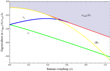
Figure 4. (Color online) The eigenvalues of $A$ associated with everywhere continuous eigenfunctions. The point-interaction strength $\gamma=-1$ and the spin-orbit-coupling strength $\eta=0.6$ (in $\hbar=c=1$ units). In figure, red line shows the border $\inf\sigma_{\mathrm{ess}}(A)$ of the essential spectrum of $A$ (Lemma IV.2). The blue $\lambda_{+}$ (green $\lambda_{-}$) line, showing the bound state as a function of the Raman coupling $\Omega\geq 0$, corresponds to the eigenfunction with a zero-valued lower (upper) component at the origin $x=0$ (Theorem V.1). The eigenvalue $\lambda_{+}$ approaches $\inf\sigma_{\mathrm{ess}}(A)=-\Omega/2$ at $\Omega=\eta^{2}+\gamma^{2}/4$ and then disappears (for details, refer to Remark V.3). Resonant states of $A$ are drawn by the yellow curve (R).

Proof of Theorem V.1.

First off, we note that, for $\lambda\in\sigma_{\mathrm{disc}}(A)$, $\lambda\neq\lambda_{0}$ due to Lemma IV.2-(i). Next, combining (II.8) with Lemma IV.2-(i) we immediately infer (see also the proof of Lemma IV.2-(i) and in particular (IV.2)) item (2) of the theorem. But then, it holds $f(0_{+})=f(0_{-})\equiv f(0)$. By solving $(I\text{\large$\otimes$}I+\gamma(A^{0}-\lambda\text{\large$\otimes$}I)^{-1}(0))f(0)=0$, we recover $\sigma_{\mathrm{disc}}(B)\backslash\sigma_{\mathrm{so}}(A)$ ($\sigma_{\mathrm{so}}(B)=\sigma_{\mathrm{so}}(A)$ by Theorem IV.4-(viii)).

In order to accomplish the proof of (1), it therefore remains to establish $\mathrm{ker}(\lambda\text{\large$\otimes$}I-A)$ ($\lambda\in\sigma_{\mathrm{disc}}(A)\backslash\sigma_{\mathrm{so}}(A)$) thus proving that items (3a)–(3b) yield $\sigma_{\mathrm{disc}}(A)=\sigma_{\mathrm{disc}}(B)$, which in turn is found by computing the poles of $R_{z}(A)$ in Lemma IV.2-(i).

We solve the characteristic equation for $H_{0}f=\lambda f$; see (II.7). Then

$$f(x)= \left(\begin{matrix}c_{1}\\ c_{3}\end{matrix}\right)e^{k_{1}x}+\left(\begin{matrix}c_{2}\\ c_{4}\end{matrix}\right)e^{k_{2}x}\quad(x>0;c_{1},\ldots,c_{4}\in\varmathbb{C};\mathrm{Re}\>k_{j}<0;j=1,2),$$

$$= \left(\begin{matrix}\tilde{c}_{1}\\ \tilde{c}_{3}\end{matrix}\right)e^{-k_{1}x}+\left(\begin{matrix}\tilde{c}_{2}\\ \tilde{c}_{4}\end{matrix}\right)e^{-k_{2}x}\quad(x<0;\tilde{c}_{1},\ldots,\tilde{c}_{4}\in\varmathbb{C};\mathrm{Re}\>k_{j}<0;j=1,2),$$ (V.4)

where

$$k_{ss^{\prime}}=s^{\prime}\sqrt{-\lambda-\eta^{2}/2+is\eta\sqrt{\lambda_{0}-\lambda}}\quad(\lambda_{0}=-(\eta^{2}+(\Omega/\eta)^{2})/4)$$ (V.5)

($k_{1}\equiv k_{+-};k_{2}\equiv k_{-,s^{\prime}};s,s^{\prime}=\pm 1;\eta>0$). The condition $\mathrm{Re}\>k_{j}<0$ ($j=1,2$) is due to $f\in D(A)$ (recall (II.5)). The boundary condition in $D(A)$, provided $f(0_{+})=f(0_{-})$, yields

$$\left(\begin{matrix}c_{1}+c_{2}\\ c_{3}+c_{4}\end{matrix}\right)=\left(\begin{matrix}\tilde{c}_{1}+\tilde{c}_{2}\\ \tilde{c}_{3}+\tilde{c}_{4}\end{matrix}\right),\quad\gamma\left(\begin{matrix}c_{1}+c_{2}\\ c_{3}+c_{4}\end{matrix}\right)=\left(\begin{matrix}k_{1}(c_{1}+\tilde{c}_{1})+k_{2}(c_{2}+\tilde{c}_{2})\\ k_{1}(c_{3}+\tilde{c}_{3})+k_{2}(c_{4}+\tilde{c}_{4})\end{matrix}\right).$$ (V.6)

We now substitute obtained functions $f$ in $H_{0}f=\lambda f$ and find that

$$c_{1}(k_{1}^{2}+\lambda-\Omega/2)+c_{3}\eta k_{1}=0,\quad c_{2}(k_{2}^{2}+\lambda-\Omega/2)+c_{4}\eta k_{2}=0,$$

$$c_{3}(k_{1}^{2}+\lambda+\Omega/2)-c_{1}\eta k_{1}=0,\quad c_{4}(k_{2}^{2}+\lambda+\Omega/2)-c_{2}\eta k_{2}=0,$$

$$\tilde{c}_{1}(k_{1}^{2}+\lambda-\Omega/2)-\tilde{c}_{3}\eta k_{1}=0,\quad\tilde{c}_{2}(k_{2}^{2}+\lambda-\Omega/2)-\tilde{c}_{4}\eta k_{2}=0,$$

$$\tilde{c}_{3}(k_{1}^{2}+\lambda+\Omega/2)+\tilde{c}_{1}\eta k_{1}=0,\quad\tilde{c}_{4}(k_{2}^{2}+\lambda+\Omega/2)+\tilde{c}_{2}\eta k_{2}=0.$$ (V.7)

We need to solve the system of equations (V.6)–(V.7). In particular, one finds from (V.7),

$$c_{3}=c_{1}Y_{1}^{(1)},\quad c_{4}=c_{2}Y_{2}^{(2)},\quad\tilde{c}_{3}=\tilde{c}_{1}Y_{3}^{(1)},\quad\tilde{c}_{4}=\tilde{c}_{2}Y_{4}^{(2)},$$ (V.8)

where

$$Y_{j}^{(s)}=\frac{a_{j}\Omega+b_{j}\sqrt{\Omega^{2}-(2\eta k_{s})^{2}}}{2\eta k_{s}}\quad(j=1,\ldots,4;s=1,2),$$ (V.9)

and $a_{1}=a_{2}=+1$, $a_{3}=a_{4}=-1$, $b_{j}=\pm 1$ for all $j=1,\ldots,4$. Hence $Y_{j}^{(s)}=-ib_{j}$ for $\Omega=0$.

For example, let $j=1$, $s=1$. From the first and third equations in (V.7) one gets that

$$\left\{\begin{array}[]{l}c_{1}(k_{1}^{2}+\lambda-\Omega/2)+c_{3}\eta k_{1}=0,\\ \\ c_{3}(k_{1}^{2}+\lambda+\Omega/2)-c_{1}\eta k_{1}=0\end{array}\right.\Longrightarrow\left\{\begin{array}[]{l}c_{1}c_{3}(k_{1}^{2}+\lambda-\Omega/2)+c_{3}^{2}\eta k_{1}=0,\\ \\ c_{1}c_{3}(k_{1}^{2}+\lambda+\Omega/2)-c_{1}^{2}\eta k_{1}=0\end{array}\right.$$

$$\Longrightarrow c_{1}c_{3}\Omega=\eta k_{1}(c_{1}^{2}+c_{3}^{2})\Longrightarrow c_{3}=c_{1}Y_{1}^{(1)},$$

and similarly for the remaining $j=2,3,4$.

By (V.8)–(V.9), there are $2^{4}=16$ possible solutions with respect to $a_{j}$ and $b_{j}$ for $j=1,\ldots,4$. These are tabulated in Tab. 1.

The number of distributions in Tab. 1 must be reduced with the help of (V.6). By (V.6), one can express $\tilde{c}_{j}$ in terms of $c_{j}$ ($j=1,\ldots,4$). Namely,

Table 1. All possible solutions of (V.7) with respect to $\{c_{3},c_{4},\tilde{c}_{3},\tilde{c}_{4}\}$ for $a_{j}$, $b_{j}=\pm 1$ for $j=1,\ldots,4$ given in (V.8)–(V.9).

$N$	$a_{1}$	$b_{1}$	$a_{2}$	$b_{2}$	$a_{3}$	$b_{3}$	$a_{4}$	$b_{4}$	$b_{1}-b_{3}$	$b_{2}-b_{3}$	$b_{1}-b_{4}$	$b_{2}-b_{4}$
$1$	$+$	$-$	$+$	$-$	$-$	$-$	$-$	$-$	$\mathrm{𝟎}$	$\mathrm{𝟎}$	$\mathrm{𝟎}$	$\mathrm{𝟎}$
$2$	$+$	$-$	$+$	$-$	$-$	$-$	$-$	$+$	$\mathrm{𝟎}$	$\mathrm{𝟎}$	$-2$	$-2$
$3$	$+$	$-$	$+$	$-$	$-$	$+$	$-$	$-$	$-2$	$-2$	$\mathrm{𝟎}$	$\mathrm{𝟎}$
$4$	$+$	$-$	$+$	$-$	$-$	$+$	$-$	$+$	$-2$	$-2$	$-2$	$-2$
$5$	$+$	$-$	$+$	$+$	$-$	$-$	$-$	$-$	$\mathrm{𝟎}$	$+2$	$\mathrm{𝟎}$	$+2$
$6$	$+$	$-$	$+$	$+$	$-$	$-$	$-$	$+$	$\mathrm{𝟎}$	$+2$	$-2$	$\mathrm{𝟎}$
$7$	$+$	$-$	$+$	$+$	$-$	$+$	$-$	$-$	$-2$	$\mathrm{𝟎}$	$\mathrm{𝟎}$	$+2$
$8$	$+$	$-$	$+$	$+$	$-$	$+$	$-$	$+$	$-2$	$\mathrm{𝟎}$	$-2$	$\mathrm{𝟎}$
$9$	$+$	$+$	$+$	$-$	$-$	$-$	$-$	$-$	$+2$	$\mathrm{𝟎}$	$+2$	$\mathrm{𝟎}$
$10$	$+$	$+$	$+$	$-$	$-$	$-$	$-$	$+$	$+2$	$\mathrm{𝟎}$	$\mathrm{𝟎}$	$-2$
$11$	$+$	$+$	$+$	$-$	$-$	$+$	$-$	$-$	$\mathrm{𝟎}$	$-2$	$+2$	$\mathrm{𝟎}$
$12$	$+$	$+$	$+$	$-$	$-$	$+$	$-$	$+$	$\mathrm{𝟎}$	$-2$	$\mathrm{𝟎}$	$-2$
$13$	$+$	$+$	$+$	$+$	$-$	$-$	$-$	$-$	$+2$	$+2$	$+2$	$+2$
$14$	$+$	$+$	$+$	$+$	$-$	$-$	$-$	$+$	$+2$	$+2$	$\mathrm{𝟎}$	$\mathrm{𝟎}$
$15$	$+$	$+$	$+$	$+$	$-$	$+$	$-$	$-$	$\mathrm{𝟎}$	$\mathrm{𝟎}$	$+2$	$+2$
$16$	$+$	$+$	$+$	$+$	$-$	$+$	$-$	$+$	$\mathrm{𝟎}$	$\mathrm{𝟎}$	$\mathrm{𝟎}$	$\mathrm{𝟎}$

$$\tilde{c}_{1}(k_{1}-k_{2})=c_{1}(\gamma-k_{1}-k_{2})+c_{2}(\gamma-2k_{2}),$$

$$\tilde{c}_{2}(k_{1}-k_{2})=c_{1}(2k_{1}-\gamma)+c_{2}(k_{1}+k_{2}-\gamma),$$ (V.10a)

and

$$\tilde{c}_{3}(k_{1}-k_{2})=c_{3}(\gamma-k_{1}-k_{2})+c_{4}(\gamma-2k_{2}),$$

$$\tilde{c}_{4}(k_{1}-k_{2})=c_{3}(2k_{1}-\gamma)+c_{4}(k_{1}+k_{2}-\gamma).$$ (V.10b)

By (V.8), substitute $\tilde{c}_{3}$, $c_{3}$ and $c_{4}$ in the first equation of (V.10b) and get

$$\tilde{c}_{1}Y_{3}^{(1)}(k_{1}-k_{2})=c_{1}Y_{1}^{(1)}(\gamma-k_{1}-k_{2})+c_{2}Y_{2}^{(2)}(\gamma-2k_{2}).$$

Now multiply the first equation of (V.10a) by $Y_{3}^{(1)}$ and subtract both obtained equations so that $\tilde{c}_{1}$ is eliminated,

$$0=c_{1}(\gamma-k_{1}-k_{2})\bigl{(}Y_{1}^{(1)}-Y_{3}^{(1)}\bigr{)}+c_{2}(\gamma-2k_{2})\bigl{(}Y_{2}^{(2)}-Y_{3}^{(1)}\bigr{)}.$$ (V.11a)

Similarly, by using (V.8), substitute $\tilde{c}_{4}$, $c_{3}$ and $c_{4}$ in the second equation of (V.10b) and get

$$\tilde{c}_{2}Y_{4}^{(2)}(k_{1}-k_{2})=c_{1}Y_{1}^{(1)}(2k_{1}-\gamma)+c_{2}Y_{2}^{(2)}(k_{1}+k_{2}-\gamma).$$

Multiply the second equation of (V.10a) by $Y_{4}^{(2)}$ and subtract both obtained equations so that $\tilde{c}_{2}$ is eliminated,

$$0=c_{1}(2k_{1}-\gamma)\bigl{(}Y_{1}^{(1)}-Y_{4}^{(2)}\bigr{)}+c_{2}(k_{1}+k_{2}-\gamma)\bigl{(}Y_{2}^{(2)}-Y_{4}^{(2)}\bigr{)}.$$ (V.11b)

By using (V.9), equations (V.11) can be rewritten explicitly as follows

$$0= c_{1}k_{2}(\gamma-k_{1}-k_{2})\bigl{(}2\Omega+(b_{1}-b_{3})\bigl{(}\Omega^{2}-(2\eta k_{1})^{2}\bigr{)}^{\frac{1}{2}}\bigr{)}$$

$$+c_{2}(\gamma-2k_{2})\bigl{(}\Omega(k_{1}+k_{2})+b_{2}k_{1}\bigl{(}\Omega^{2}-(2\eta k_{2})^{2}\bigr{)}^{\frac{1}{2}}$$

$$-b_{3}k_{2}\bigl{(}\Omega^{2}-(2\eta k_{1})^{2}\bigr{)}^{\frac{1}{2}}\bigr{)},$$

and

$$0= c_{1}(2k_{1}-\gamma)\bigl{(}\Omega(k_{1}+k_{2})+b_{1}k_{2}\bigl{(}\Omega^{2}-(2\eta k_{1})^{2}\bigr{)}^{\frac{1}{2}}$$

$$-b_{4}k_{1}\bigl{(}\Omega^{2}-(2\eta k_{2})^{2}\bigr{)}^{\frac{1}{2}}\bigr{)}+c_{2}k_{1}(k_{1}+k_{2}-\gamma)\bigl{(}2\Omega$$

$$+(b_{2}-b_{4})\bigl{(}\Omega^{2}-(2\eta k_{2})^{2}\bigr{)}^{\frac{1}{2}}\bigr{)}.$$

By noting that $c_{1}$ and $c_{2}$ are two independent constants, we can subtract both equations and separate the expressions at $c_{1}$ and $c_{2}$ one from another. Then

$$E_{\Omega}(k_{1},k_{2})\equiv 0,\quad\varphi E_{\Omega}(k_{1},k_{2})\equiv 0,$$

where

$$E_{\Omega}(k_{1},k_{2})= \Omega[\gamma(k_{1}+3k_{2})-2(k_{1}+k_{2})^{2}]+b_{4}k_{1}(2k_{1}-\gamma)[\Omega^{2}-(2\eta k_{2})^{2}]^{\frac{1}{2}}$$

$$+k_{2}[b_{3}(k_{1}+k_{2}-\gamma)-b_{1}(3k_{1}+k_{2}-2\gamma)][\Omega^{2}-(2\eta k_{1})^{2}]^{\frac{1}{2}},$$

with a one-to-one map $\varphi\!\colon\thinspace k_{1}\mapsto k_{2}$, $k_{2}\mapsto k_{1}$, $b_{1}\mapsto b_{2}$, $b_{2}\mapsto b_{1}$, $b_{3}\mapsto b_{4}$, and $b_{4}\mapsto b_{3}$. Then $\varphi^{n}=I$ (identity) for $n=0,2,4,\ldots$, and $\varphi^{n}=\varphi$ for $n=1,3,5,\ldots$ Equation $E_{0}\equiv 0$ holds for the distributions (Tab. 1) numbered by $N=2$, $4$, $6$, $8$ and $9$, $11$, $13$, $15$. On the other hand, $E_{\Omega}$ with $\Omega>0$ is well defined for $N=2$, $6$ and $11$, $15$. Therefore, we deduce that for $\Omega\geq 0$, $E_{\Omega}$ makes sense if $N=2$, $6$ and $11$, $15$.

Expression $E_{\Omega}$ can be represented by the sum of $F_{\Omega}$ and $G_{\Omega}$, where both $F_{\Omega}$ and $G_{\Omega}$ are invariant under the action of $\varphi$, namely,

$$F_{\Omega}(k_{1},k_{2})=\Omega(k_{1}+k_{2})[\gamma-2(k_{1}+k_{2})],\quad\varphi F_{\Omega}(k_{1},k_{2})=F_{\Omega}(k_{1},k_{2}),$$

and $G_{\Omega}$ is defined by

$$G_{\Omega}(k_{1},k_{2})= 2\gamma\Omega k_{2}+b_{4}k_{1}(2k_{1}-\gamma)[\Omega^{2}-(2\eta k_{2})^{2}]^{\frac{1}{2}}$$

$$+k_{2}[b_{3}(k_{1}+k_{2}-\gamma)-b_{1}(3k_{1}+k_{2}-2\gamma)][\Omega^{2}-(2\eta k_{1})^{2}]^{\frac{1}{2}}.$$

Then $G_{\Omega}$ satisfies

$$G_{\Omega}(k_{1},k_{2})=\varphi G_{\Omega}(k_{1},k_{2})=-F_{\Omega}(k_{1},k_{2})\quad(\text{since }E_{\Omega}\equiv 0)$$

and

$$\varphi^{n}G_{\Omega}(k_{1},k_{2})=G_{\Omega}(k_{1},k_{2})\quad\text{for} \quad n=0,2,4,\ldots,$$

$$\varphi^{n}G_{\Omega}(k_{1},k_{2})=\varphi G_{\Omega}(k_{1},k_{2})\quad\text{for} \quad n=1,3,5,\ldots$$

Then $(\varphi-I)G_{\Omega}=0$ yields

$$(\varphi-I)G_{\Omega}(k_{1},k_{2})= 2\gamma\Omega(k_{1}-k_{2})+k_{2}[b_{1}(3k_{1}+k_{2}-2\gamma)-b_{3}(k_{1}-k_{2})]$$

$$\times[\Omega^{2}-(2\eta k_{1})^{2}]^{\frac{1}{2}}-k_{1}[b_{2}(3k_{2}+k_{1}-2\gamma)$$

$$+b_{4}(k_{1}-k_{2})][\Omega^{2}-(2\eta k_{2})^{2}]^{\frac{1}{2}}=0.$$ (V.12)

Equation (V.12) shows that, depending on $16$ distributions in Tab. 1, four distinct classes can be considered.

$$(I):\>E_{\Omega}^{(1)}(k_{1},k_{2})\equiv 0,\;\text{with}\;\;E_{\Omega}^{(1)}(k_{1},k_{2})=\gamma\Omega(k_{1}-k_{2})$$

$$+(k_{1}+k_{2}-\gamma)\Bigl{(}b_{1}k_{2}[\Omega^{2}-(2\eta k_{1})^{2}]^{\frac{1}{2}}-b_{2}k_{1}[\Omega^{2}-(2\eta k_{2})^{2}]^{\frac{1}{2}}\Bigr{)}$$ (V.13a)

($$b_{1}=b_{3} b_{2}=b_{4}$$, ),

$$(II):\>E_{\Omega}^{(2)}(k_{1},k_{2})\equiv 0,\;\text{with}\;\;E_{\Omega}^{(2)}(k_{1},k_{2})=\gamma\Omega(k_{1}-k_{2})$$

$$+b_{1}k_{2}(k_{1}+k_{2}-\gamma)[\Omega^{2}-(2\eta k_{1})^{2}]^{\frac{1}{2}}-b_{2}k_{1}(2k_{2}-\gamma)[\Omega^{2}-(2\eta k_{2})^{2}]^{\frac{1}{2}}$$ (V.13b)

($$b_{1}=b_{3} b_{2}=-b_{4}$$, ),

$$(III):\>E_{\Omega}^{(3)}(k_{1},k_{2})\equiv 0,\;\text{with}\;\;E_{\Omega}^{(3)}(k_{1},k_{2})=-\varphi_{1}E_{\Omega}^{(2)}(k_{1},k_{2})$$ (V.13c)

($$b_{1}=-b_{3} b_{2}=b_{4} \varphi_{1}\!\colon\thinspace k_{1}\mapsto k_{2} k_{2}\mapsto k_{1} b_{1}\mapsto b_{2} b_{2}\mapsto b_{1}$$, and , , , ),

$$(IV):\>E_{\Omega}^{(4)}(k_{1},k_{2})\equiv 0,\;\text{with}\;\;E_{\Omega}^{(4)}(k_{1},k_{2})=\gamma\Omega(k_{1}-k_{2})$$

$$+b_{1}k_{2}(2k_{1}-\gamma)[\Omega^{2}-(2\eta k_{1})^{2}]^{\frac{1}{2}}-b_{2}k_{1}(2k_{2}-\gamma)[\Omega^{2}-(2\eta k_{2})^{2}]^{\frac{1}{2}}$$ (V.13d)

($b_{1}=-b_{3}$, $b_{2}=-b_{4}$).

By the isomorphism in (V.13c), it suffices to consider three classes: $(I)$, $(II)$, $(IV)$.

Class $(I)$. Given $\Omega>0$, the equation $E_{\Omega}^{(1)}\equiv 0$ (V.13a) holds for the distributions numbered by $N=1$, $6$, $11$ and $16$. If, however, $\Omega=0$, then $E_{0}^{(1)}\equiv 0$ holds for all $k_{1}$, $k_{2}$, which is inconsistent with the point spectrum of $A$. Subsequently, class $(I)$ is improper.

Class $(II)$. For $\Omega>0$, $E_{\Omega}^{(2)}\equiv 0$ (V.13b) holds for the distributions numbered by $N=2$, $5$, $12$ and $15$. Due to the isomorphism $\varphi_{1}$, the number of distributions decreases to $N=2$, $3$, $5$, $8$, $9$, $12$, $14$ and $15$. But $E_{0}^{(2)}\equiv 0$ yields $k_{1}(k_{1}+k_{2}-2\gamma)+k_{2}(k_{1}-3k_{2}+2\gamma)=0$ which is satisfied only for $k_{1}=k_{2}=\gamma/2$, hence improper due to $\lambda\neq\lambda_{0}$.

Class $(IV)$. For $\Omega>0$, $E_{\Omega}^{(4)}\equiv 0$ (V.13d) holds for the distributions numbered by $N=4$, $7$, $10$ and $13$. For $\Omega=0$, $E_{0}^{(4)}\equiv 0$ yields a correct relation $k_{1}+k_{2}=\gamma$. Possible distributions are numbered by $N=7$ and $N=10$.

As a result, we have found that $E_{\Omega}^{(4)}\equiv 0$ is the only one correct equation which holds for all $\Omega\geq 0$. The associated distributions in Tab. 1 are numbered by $N=7$ and $10$.

By solving (V.13d), we find that

$$k_{1}+k_{2}=\gamma(1+\chi_{\Omega}),$$ (V.14)

where

$$\chi_{\Omega}=\Omega\cdot\frac{-\gamma^{2}\Omega+2k_{1}k_{2}\bigl{(}\Omega\pm[\Omega^{2}-(\gamma\eta)^{2}+(2\eta)^{2}k_{1}k_{2}]^{\frac{1}{2}}\bigr{)}}{2[(2\eta k_{1}k_{2})^{2}+(\gamma\Omega)^{2}]}$$ (V.15)

($\Omega,\eta\geq 0$), $\chi_{0}=0$ and $\gamma<0$. As it should be by (V.12), equation (V.14) is invariant under the action of $\varphi$ as well as $\varphi_{1}$.

Recalling that $k_{1}k_{2}=s^{\prime}[\lambda^{2}-(\Omega/2)^{2}]^{1/2}$ ($s^{\prime}=\pm 1$), one can construct the equation for the eigenvalues $\lambda$. By (V.14), $\lambda$ satisfies the following cubic equation

$$(8\eta)^{2}\lambda^{3}+16[\eta^{2}(\gamma^{2}+\eta^{2})+\Omega(\Omega\pm 4\eta^{2})]\lambda^{2}$$

$$\pm 8\Omega[2\Omega^{2}+(\gamma^{2}+2\eta^{2})(\eta^{2}\pm\Omega)]\lambda+\Omega^{2}[4\eta^{4}+(\gamma^{2}\pm 2\Omega)^{2}]=0$$ (V.16)

($\Omega\geq 0$), provided $\mathrm{Re}\>k_{j}<0$ for $j=1,2$. Note that the sign $\pm$ corresponds to that in (V.15).

Now, it is necessary to show that the eigenvalues $\lambda$, which satisfy (V.16), are also in $\sigma_{\mathrm{disc}}(B)\backslash\sigma_{\mathrm{so}}(A)$, thus accomplishing the proof of Theorem V.1-(1), and that the eigenfunctions of $\sigma_{\mathrm{disc}}(A)\backslash\sigma_{\mathrm{so}}(A)$ are as in (V.1)–(V.2), thus giving Theorem V.1-(3a) and (3b).

We solve (V.7) with respect to $c_{3}$, $c_{4}$ and $\tilde{c}_{3}$, $\tilde{c}_{4}$, by assuming that $\eta>0$,

$$c_{3}= c_{1}\>\frac{\eta k_{1}}{k_{1}^{2}+\lambda+\Omega/2}=-c_{1}\>\frac{k_{1}^{2}+\lambda-\Omega/2}{\eta k_{1}},$$

$$c_{4}= c_{2}\>\frac{\eta k_{2}}{k_{2}^{2}+\lambda+\Omega/2}=-c_{2}\>\frac{k_{2}^{2}+\lambda-\Omega/2}{\eta k_{2}},$$

$$\tilde{c}_{3}= -\tilde{c}_{1}\>\frac{\eta k_{1}}{k_{1}^{2}+\lambda+\Omega/2}=\tilde{c}_{1}\>\frac{k_{1}^{2}+\lambda-\Omega/2}{\eta k_{1}},$$

$$\tilde{c}_{4}= -\tilde{c}_{2}\>\frac{\eta k_{2}}{k_{2}^{2}+\lambda+\Omega/2}=\tilde{c}_{2}\>\frac{k_{2}^{2}+\lambda-\Omega/2}{\eta k_{2}}.$$

We note that each equality in every row can be chosen arbitrarily; we choose the first one. Substitute obtained expressions in (V.4) and find by (V.6),

$$f(0_{+})=c_{1}\left(\begin{matrix}1\\ \frac{\eta k_{1}}{k_{1}^{2}+\lambda+\Omega/2}\end{matrix}\right)+c_{2}\left(\begin{matrix}1\\ \frac{\eta k_{2}}{k_{2}^{2}+\lambda+\Omega/2}\end{matrix}\right),\;\;f(0_{-})=\tilde{c}_{1}\left(\begin{matrix}1\\ \frac{-\eta k_{1}}{k_{1}^{2}+\lambda+\Omega/2}\end{matrix}\right)+\tilde{c}_{2}\left(\begin{matrix}1\\ \frac{-\eta k_{2}}{k_{2}^{2}+\lambda+\Omega/2}\end{matrix}\right),$$

$$f^{\prime}(0_{+})=c_{1}\left(\begin{matrix}k_{1}\\ \frac{\eta k_{1}^{2}}{k_{1}^{2}+\lambda+\Omega/2}\end{matrix}\right)+c_{2}\left(\begin{matrix}k_{2}\\ \frac{\eta k_{2}^{2}}{k_{2}^{2}+\lambda+\Omega/2}\end{matrix}\right),\;\;f^{\prime}(0_{-})=\tilde{c}_{1}\left(\begin{matrix}-k_{1}\\ \frac{\eta k_{1}^{2}}{k_{1}^{2}+\lambda+\Omega/2}\end{matrix}\right)+\tilde{c}_{2}\left(\begin{matrix}-k_{2}\\ \frac{\eta k_{2}^{2}}{k_{2}^{2}+\lambda+\Omega/2}\end{matrix}\right).$$

These functions, with $f(0_{+})=f(0_{-})$, are in $D(A)$. Hence the boundary condition given by $\gamma(f(0_{+})+f(0_{-}))/2=f^{\prime}(0_{+})-f^{\prime}(0_{-})$ yields

$$0= (c_{1}+c_{2})\left(\gamma-\frac{2k_{1}k_{2}(k_{1}+k_{2})}{k_{1}k_{2}-\lambda-\Omega/2}\right),$$ (V.17a)

$$0= \eta(c_{1}-\tilde{c}_{1})\left(\frac{k_{1}(2k_{1}-\gamma)}{k_{1}^{2}+\lambda+\Omega/2}-\frac{k_{2}(2k_{2}-\gamma)}{k_{2}^{2}+\lambda+\Omega/2}\right).$$ (V.17b)

By (V.17), four possible cases are then considered, provided $\eta>0$:

Case (1). $c_{1}+c_{2}=0$ and $c_{1}-\tilde{c}_{1}=0$. By (V.4), $c_{1}+c_{2}=\tilde{c}_{1}+\tilde{c}_{2}=0$. Hence $\tilde{c}_{2}=-\tilde{c}_{1}=-c_{1}$. By (V.6), $\tilde{c}_{2}(k_{1}-k_{2})=c_{1}(2k_{1}-\gamma)+c_{2}(k_{1}+k_{2}-\gamma)$ (see also (V.10a)). Hence $c_{1}(k_{1}-k_{2})=0$. If $c_{1}=0$, then $f\equiv 0$, hence trivial. If $k_{1}=k_{2}$, then $\lambda=\lambda_{0}$, by (V.5), and $f\equiv 0$, by (V.4); hence improper again.

Case (2).

$$c_{1}+c_{2}=0\quad\text{and}\quad\frac{k_{1}(2k_{1}-\gamma)}{k_{1}^{2}+\lambda+\Omega/2}-\frac{k_{2}(2k_{2}-\gamma)}{k_{2}^{2}+\lambda+\Omega/2}=0\Longrightarrow\gamma=-\frac{2(k_{1}+k_{2})(\lambda+\Omega/2)}{k_{1}k_{2}-\lambda-\Omega/2}.$$

If we expand the latter equation by using (V.5), this agrees with (V.16) for the upper sign. By noting that $k_{j}=ip_{j}$ for $j=1,2$, and $p_{j}$ as in the theorem, we find that the correspondence is one-to-one with the eigenvalues in $\sigma_{\mathrm{disc}}(B)\backslash\sigma_{\mathrm{so}}(A)$ obtained by setting the lower sign.

By (V.4), $c_{1}+c_{2}=\tilde{c}_{1}+\tilde{c}_{2}=0$, and thus $\tilde{c}_{2}=-\tilde{c}_{1}$. Then (V.10a) yields $\tilde{c}_{1}=-c_{1}$ and $\tilde{c}_{2}=c_{1}$. The substitution of these coefficients in (V.4) gives (V.2), with $k_{j}=ip_{j}$ ($j=1,2$), $C\equiv c_{1}\in\varmathbb{C}$.

Case (3).

$$\gamma-\frac{2k_{1}k_{2}(k_{1}+k_{2})}{k_{1}k_{2}-\lambda-\Omega/2}=0\quad\text{and}\quad c_{1}-\tilde{c}_{1}=0.$$

Similarly to the previous case, by expanding the former equation with the help of (V.5), we establish (V.16) with the lower sign. Subsequently, this corresponds to the upper sign in $\sigma_{\mathrm{disc}}(B)\backslash\sigma_{\mathrm{so}}(A)$.

The latter equation, $c_{1}-\tilde{c}_{1}=0$, along with (V.4) yields

$$\tilde{c}_{1}=c_{1},\quad\tilde{c}_{2}=c_{2}=-c_{1}\>\frac{k_{1}}{k_{2}}\cdot\frac{k_{2}^{2}+\lambda+\Omega/2}{k_{1}^{2}+\lambda+\Omega/2}.$$

Substitute obtained coefficients in (V.4) and get (V.1), with $k_{j}=ip_{j}$ ($j=1,2$) and the coefficient $C\equiv c_{1}p_{1}/(\lambda+\Omega/2-p_{1}^{2})\in\varmathbb{C}$ (note that the denominator is nonzero unless $\lambda$ is in the essential spectrum).

Case (4).

$$\gamma=\frac{2k_{1}k_{2}(k_{1}+k_{2})}{k_{1}k_{2}-\lambda-\Omega/2}\quad\text{and}\quad\gamma=-\frac{2(k_{1}+k_{2})(\lambda+\Omega/2)}{k_{1}k_{2}-\lambda-\Omega/2}.$$

The combination of both equations yields $(k_{1}+k_{2})(k_{1}k_{2}+\lambda+\Omega/2)=0$. If $k_{1}k_{2}+\lambda+\Omega/2=0$, then, recalling that (refer to (V.5)) $k_{1}k_{2}=s^{\prime}\sqrt{\lambda^{2}-(\Omega/2)^{2}}$ ($s^{\prime}=\pm 1$), it holds $\lambda=-\Omega/2$, hence improper. If, however, $k_{1}+k_{2}=0$, then $\lambda=\lambda_{0}$, by (V.5), hence improper again.

As a result, Cases (2)–(3) accomplish the proof of items (1) and (3a)–(3b) of Theorem V.1.

We now concentrate on (3c). For $\eta=0$, equation $H_{0}f=\lambda f$, $f\in D(A)$, is easy to deal with since the components $f_{1}$ and $f_{2}$ are separated and thus can be solved independently one from another: $f_{1}^{\prime\prime}+(\lambda-\Omega/2)f_{1}=0$, $f_{2}^{\prime\prime}+(\lambda+\Omega/2)f_{2}=0$. By substituting obtained exponents in the boundary condition we get (3c). Moreover, the condition $\gamma<-2\sqrt{\Omega}$ is obtained from the inspection of the resolvent in Lemma IV.2-(i), where one requires $\mathrm{Im}\>p_{j}>0$ for $j=1,2$. For $\eta=0$, $z<-\Omega/2$, and hence $-\gamma^{2}/4+\Omega/2<-\Omega/2$ thus yielding $\gamma<-2\sqrt{\Omega}$. Otherwise, only one eigenvalue $-\gamma^{2}/4-\Omega/2$ remains.

In particular, this also proves that $(\sigma_{\mathrm{disc}}(A)\backslash\sigma_{\mathrm{so}}(A))\cap\sigma_{\mathrm{ess}}(A)=\varnothing$ (see item (4) of the theorem) for $\eta=0$, since $J(0,\Omega)=-\Omega/2$. For arbitrary spin-orbit coupling $\eta>0$, let us examine the conditions $\mathrm{Im}\>p_{j}>0$ for $j=1,2$. It suffices to show the converse for at least one $p_{j}$.

Let $j=1$ and $0<\Omega\leq\eta^{2}$. Then $J(\eta,\Omega)=\lambda_{0}$. Assume that the eigenvalue $\lambda=\lambda_{0}+\nu$ for some real $\nu>0$. Then it holds $p_{1}=\sqrt{\lambda_{0}+\nu+\eta^{2}/2+\eta\sqrt{\nu}}$. But $\lambda_{0}+\eta^{2}/2=(\eta^{4}-\Omega^{2})/(4\eta^{2})\geq 0$ for all $0<\Omega\leq\eta^{2}$. Hence $\mathrm{Im}\>p_{1}=0$, which is invalid.

Let $j=1$ and $\Omega>\eta^{2}>0$. Then $J(\eta,\Omega)=-\Omega/2$. Let $\lambda=-\Omega/2+\nu$ for some $\nu>0$. Then we have that $p_{1}=\sqrt{-a+\nu+\sqrt{a^{2}+\eta^{2}\nu}}$, where $a=(\Omega-\eta^{2})/2>0$ for all $\Omega>\eta^{2}>0$. As seen, $\mathrm{Im}\>p_{1}=0$ for all $0<\nu\leq\Omega$. Next, let $\nu=\Omega+\mu$ for some $\mu>0$, and substitute $\lambda=\Omega/2+\mu$ in (V.16). One gets that

$$0= \eta^{4}\Omega^{2}+8\eta^{2}(\Omega+\mu)(\Omega^{2}+\eta^{2}(\Omega+2\mu))+16(\Omega+\mu)^{2}(\eta^{4}+\Omega^{2}+2\eta^{2}(\Omega+2\mu)),$$

for the lower sign, and that

$$0= 16\eta^{2}\mu^{2}(\gamma^{2}+\eta^{2}+4\mu)+8\eta^{2}\mu\Omega(\gamma^{2}+4\mu)+\Omega^{2}(\gamma^{2}+4\mu)^{2}$$

for the upper one. It is evident that the above equations do not have real solutions for all $\mu>0$ for all $\Omega,\eta>0$ ($\gamma<0$), since all the terms on the right-hand side are positive, whereas the left-hand side is zero. Therefore, $\mathrm{Im}\>p_{1}=0$ for $\nu>\Omega$ as well. Subsequently, item (4) holds, and this accomplishes the proof of the theorem. ∎

Remark V.3.

In Fig. 4, one finds that $\lambda_{+}$ vanishes for $\Omega\geq\eta^{2}+\gamma^{2}/4$, by substituting $\lambda=-\Omega/2$ in $\sigma_{\mathrm{disc}}(A)\backslash\sigma_{\mathrm{so}}(A)$ (Theorem V.1-(1)) or in (V.16) and solving the obtained equation with respect to $\Omega$. The suffix <<+>> indicates that the eigenvalue is found from $\sigma_{\mathrm{disc}}(A)\backslash\sigma_{\mathrm{so}}(A)$ with the plus sign (or from (V.16) with the minus sign). We also note that the condition $\lambda<\inf\sigma_{\mathrm{ess}}(A)$ alone is insufficient to derive proper bound states; this must be implemented with the requirement $\mathrm{Im}\>p_{j}>0$ for $j=1,2$ as well.

VI. Summary and discussion

In this paper, we solved the bound state problem for the spin-orbit coupled ultracold atom in a one-dimensional short-range potential describing the impurity scattering. The potential is assumed to be approximated by the $\delta$-interaction. As a result, two distinct realizations of the original differential expression, $H$, were proposed. The first one, $A$, is implemented through the boundary condition defining the domain of the operator. The second realization, $B$, has a meaning of distribution. Although both representatives provide identical spectra, the eigenfunctions differ in their form: Equivalence classes of functions of $B$ supply with insufficient information concerning the (classical) behavior of eigenfunctions.

Based on the property that $H$ contains both the spin-orbit and the Raman coupling, we showed that, for nonzero spin-orbit and Raman coupling, the spectrum is implemented with some extra states, in addition to those which are found by solving the eigenvalue equation directly. Extra states, called the spin-orbit coupling induced states, have a peculiarity that the associated eigenfunctions are discontinuous at the origin $x=0$, and that there might be a point embedded into the essential spectrum. By (dis)continuity we assume that, although functions are defined on any subset of $\varmathbb{R}\backslash\{0\}$, their left ($x=0_{-}$) and right ($x=0_{+}$) representatives either coincide (continuity) or not (discontinuity). Such states originate from the fact that the spin-orbit Hamiltonian is not purely Dirac-like or Schrödinger-like operator but rather their one-dimensional mixture. It turns out that $A$ ($B$) commutes with the operator which is unitarily equivalent to the one-dimensional Dirac operator (in Weyl’s form) for the particle with spin one-half moving in the Fermi pseudopotential $V_{F}$. In turn, we showed that $V_{F}$ is a combination of both $\delta$- and $\delta^{\prime}$-interactions, where the latter accounts for the divergent terms occurring if dealt with discontinuous functions (one has the so-called $\delta_{p}^{\prime}$-interaction).

Finally, we established the remaining part of the discrete spectrum of $A$ ($B$) and showed that the eigenvalues under consideration are found by solving the cubic equation. Depending on the regime of the Raman coupling, that is to say, on the strength of the Zeeman field, one observes either two or a single point in the spectrum. The associated eigenfunctions are everywhere continuous but with zero-valued component (either upper or lower one) at the origin.

It is worth noting that the (self-adjoint) representatives $A_{0}$ and $A$ of the atom-light coupling $U$ and the Hamiltonian $H$ could serve for a tool to recover other self-adjoint extensions thus corresponding to modified point-interactions. This could be done with the help of Krein’s formula (Krein, 1947, Eq. (6.10)) (see also (Albeverio et al., 2005, Appendix A)). For that purpose one needs to apply the resolvents of $A_{0}$ and $A$ given in Theorem III.2-(i) and Lemma IV.2-(i), respectively. Following eg Šeba (1986); Albeverio et al. (1998), one constructs operators on the intervals $(-\infty,0)$ and $(0,\infty)$, and finds the orthonormal bases relevant to deficiency subspaces. So defined, the operators have d.i. (2,2). The entries of the associated unitary matrix from $U(2)$ group thus determine all self-adjoint extensions.

References

- Adams and Fournier [2003] R. A. Adams and J. J. Fournier. Sobolev Spaces. Elsevier Science Ltd, Oxford, UK, 2 edition, 2003.
- Albeverio et al. [1998] S. Albeverio, L. Dąbrowski, and P. Kurasov. Lett. Math. Phys., 45:33, 1998.
- Albeverio et al. [2005] S. Albeverio, F. Gesztesy, R. Hoegh-Krohn, and H. Holden. Solvable Models in Quantum Mechanics. AMS Chelsea Publishing (Providence, Rhode Island), 2 edition, 2005.
- Anderson et al. [2012] Brandon M. Anderson, Gediminas Juzeliūnas, Victor M. Galitski, and I. B. Spielman. Phys. Rev. Lett., 108:235301, 2012.
- Benvegnù and Dąbrowski [1994] S. Benvegnù and L. Dąbrowski. Lett. Math. Phys., 30:159, 1994.
- Bychkov and Rashba [1984] Y. A. Bychkov and E. I. Rashba. J. Phys. C, 17:6039, 1984.
- Campbell et al. [2011] D. L. Campbell, G. Juzeliūnas, and I. B. Spielman. Phys. Rev. A, 84:025602, 2011.
- Cheuk et al. [2012] Lawrence W. Cheuk, Ariel T. Sommer, Zoran Hadzibabic, Tarik Yefsah, Waseem S. Bakr, and Martin W. Zwierlein. Phys. Rev. Lett., 109:095302, 2012.
- Coutinho et al. [1997] F. A. B. Coutinho, Y. Nogami, and J. Fernando Perez. J. Phys. A.: Math. Gen., 30:3937, 1997.
- Coutinho et al. [2004] F. A. B. Coutinho, Y. Nogami, Lauro Tomio, and F. M. Toyama. J. Phys. A.: Math. Gen., 37:10653, 2004.
- Coutinho et al. [2009] F. A. B. Coutinho, Y. Nogami, and F. M. Toyama. Rev. Bras. Ens. de Fis., 31:4302, 2009.
- Dalibard et al. [2011] Jean Dalibard, Fabrice Gerbier, Gediminas Juzeliūnas, and Patrik Öhberg. Rev. Mod. Phys., 83:1523, 2011.
- Dresselhaus [1955] G. Dresselhaus. Phys. Rev., 100(2):580, 1955.
- Galitski and Spielman [2013] Victor Galitski and Ian B. Spielman. Nature, 494:49, 2013.
- García-Ravelo et al. [2012] J. García-Ravelo, A. Schulze-Halberg, and A. L. Trujillo. J. Math. Phys., 53:102101, 2012.
- Griffiths and Walborn [1999] David Griffiths and Stephen Walborn. Am. J. Phys., 67:446, 1999.
- Griffiths [1993] David J. Griffiths. J. Phys. A.: Math. Gen., 26:2265, 1993.
- Herczyński [1989] Jan Herczyński. J. Operator Theory, 21:273, 1989.
- Hughes [1997] Rhonda J. Hughes. Rep. Math. Phys., 39(3):425, 1997.
- Juzeliūnas et al. [2010] Gediminas Juzeliūnas, Julius Ruseckas, and Jean Dalibard. Phys. Rev. A, 81:053403, 2010.
- Krein [1947] M. G. Krein. Rec. Math. (Mat. Sbornik) N.S., 20(62):431, 1947.
- Lin et al. [2009] Y.-J. Lin, R. L. Compton, K. Jiménez-García, J. V. Porto, and I. B. Spielman. Nature, 462:628, 2009.
- Lin et al. [2011] Y.-J. Lin, K. Jiménez-García, and I. B. Spielman. Nature, 471:83, 2011.
- Malamud and Schmüdgen [2012] Mark M. Malamud and Konrad Schmüdgen. J. Func. Anal., 263:3144, 2012.
- Reed and Simon [1975] M. Reed and B. Simon. Methods of Modern Mathematical Physics II: Fourier Analysis, Self-Adjointness, volume 2. Academic Press, Inc. (London) LTD., 1975.
- Reed and Simon [1980] M. Reed and B. Simon. Methods of Modern Mathematical Physics I: Functional Analysis, volume 1. Academic Press, Inc. (London) LTD., 1980.
- Šeba [1986] P. Šeba. Czech. J. Phys. B, 36:667, 1986.
- Wang et al. [2012] Pengjun Wang, Zeng-Qiang Yu, Zhengkun Fu, Jiao Miao, Lianghui Huang, Shijie Chai, Hui Zhai, and Jing Zhang. Phys. Rev. Lett., 109:095301, 2012.