Quantified Energy Dissipation Rates: Electromagnetic Wave Observations in the Terrestrial Bow Shock

Abstract

We present the first quantified measure of the rate of energy dissipated per unit volume by high frequency electromagnetic waves in the transition region of the Earth’s collisionless bow shock using data from the THEMIS spacecraft. Every THEMIS shock crossing examined with available wave burst data showed both low frequency ($<$10 Hz) magnetosonic-whistler waves and high frequency ($\gtrsim$10 Hz) electromagnetic and electrostatic waves throughout the entire transition region and into the magnetosheath. The waves in both frequency ranges had large amplitudes, but the higher frequency waves, which are the focus of this study, showed larger contributions to both the Poynting flux and the energy dissipation rates. The higher frequency waves were identified as combinations of ion-acoustic waves, electron cyclotron drift instability driven waves, electrostatic solitary waves, and whistler mode waves. These waves were found to have: (1) amplitudes capable of exceeding $\delta$B $\sim$ 10 nT and $\delta$E $\sim$ 300 mV/m, though more typical values were $\delta$B $\sim$ 0.1-1.0 nT and $\delta$E $\sim$ 10-50 mV/m; (2) energy fluxes in excess of 2000 $\mu$W m^-2; (3) resistivities $>$ 9000 $\Omega$ m; and (4) energy dissipation rates $>$ 3 $\mu$W m^-3. The dissipation rates were found to be in excess of four orders of magnitude greater than was necessary to explain the increase in entropy across the shocks. Thus, the waves need only be, at times, $<$ 0.01% efficient to balance the nonlinear wave steepening that produces the shocks. Therefore, these results show for the first time that high frequency electromagnetic and electrostatic waves have the capacity to regulate the global structure of collisionless shocks.

1 Introduction

Shock waves, in their simplest form, are discontinuities that result from the balance between nonlinear wave steepening and energy loss. The energy loss must transform the incident bulk flow kinetic energy to some other form like random kinetic energy (i.e., heat). If this energy transformation is irreversible, then the process is said to have dissipated energy [Petschek, 1958; Fishman et al., 1960]. The distinction between reversible and irreversible is important because the initiation of a shock discontinuity from a nonlinearly steepened wave requires that the transformation be irreversible [Shu, 1992]. In a collision dominated media like the Earth’s atmosphere, energy dissipation is accomplished through binary particle collisions. In a collisionless media like the solar wind, particle collisions occur too infrequently to significantly alter the incident bulk flow kinetic energy in the shock ramp. Yet, collisionless shock waves are known to be efficient mechanisms by which charged particles can be heated and/or accelerated. In addition, the basic theories for possible energy dissipation mechanisms in these shocks have remained relatively unchanged for over 40 years [e.g., Sagdeev, 1966; Coroniti, 1970; Tidman and Krall, 1971; Wu et al., 1984; Treumann, 2009]. However, the relative importance of each possible dissipation mechanism has not been quantified for low Mach number shocks.

The four possible mechanisms by which a collisionless shock could transfer energy are: wave dispersion [e.g., Mellott and Greenstadt, 1984; Krasnoselskikh et al., 2002; Sundkvist et al., 2012], wave-particle interactions [e.g., Sagdeev, 1966; Gary, 1981], particle reflection [e.g., Edmiston and Kennel, 1984; Kennel, 1987; Bale et al., 2005], and macroscopic quasi-static field effects [e.g., Scudder et al., 1986a, b, c]. Theory predicts that the dominant type of energy dissipation depends strongly upon fast mode Mach number, M_f, shock normal angle, $\theta{{}_{Bn}}$, and the ratio of particle to magnetic pressures called the plasma beta, $\beta$ [e.g., Kennel et al., 1985]. At low M_f, theory suggests that the dominant mechanisms are wave dispersion and/or wave-particle interactions [Kennel et al., 1985]. Above some critical Mach number, M_cr, the shock requires additional energy dissipation in the form of particle reflection to limit wave steepening [Edmiston and Kennel, 1984]. Numerous studies have argued that macroscopic quasi-static fields (the fourth mechanism) govern the dynamics of charged particles in low Mach number collisionless shock waves [e.g., Scudder et al., 1986c; Hull et al., 2000, 2001]. Theory and observation support the first three mechanisms, but we believe that the fourth mechanism has been given too much importance due to low resolution observations.

Recent studies have argued that quasi-static fields dominate over higher frequency waves [e.g., Dimmock et al., 2012; Mitchell et al., 2012]. However, previous observations of quasi-static electric fields were often under-sampled and/or the instrument saturated (e.g., Cluster saturates near $\sim$40 mV/m). The under-sampled electric fields often show a “spiky” signature that is assumed to be the quasi-static electric field called the cross-shock potential [e.g., Mozer and Sundkvist, 2013; Sundkvist and Mozer, 2013]. These low frequency electric field observations require a reference frame transformation to remove convective field effects. However, the observation of nonlinear ($\delta$B/B $>$ 1) electromagnetic fluctuations near the ramps of collisionless shocks [e.g., Wilson III et al., 2012; Sundkvist and Mozer, 2013] and evidence of shock reformation/non-stationarity [e.g., Lobzin et al., 2007; Mazelle et al., 2010] raise doubts about the ability to remove convective field effects. Moreover, observations [e.g., Wilson III et al., 2007, 2010] show that higher frequency wave fields can be much larger ($\gtrsim$200 mV/m) than the quasi-static electric fields typically observed ($\sim$few 10’s of mV/m) [e.g., Dimmock et al., 2012; Mozer and Sundkvist, 2013].

If the quasi-static electric fields govern the dynamics of charged particles across the shock, then, ignoring other mechanisms, the transition would be thermodynamically reversible. Of the four possible energy dissipation mechanisms in collisionless shocks, only wave-particle interactions can directly produce an irreversible change in energy. Recently, Parks et al. [2012] observed that the entropy flux density increases across the bow shock, which argues against a purely reversible transition. Previous studies that examined particle distributions in detail showed that the downstream distributions could not be explained by only assuming acceleration due to a quasi-static electric field across the shock ramp [e.g., Scudder et al., 1986c; Schwartz et al., 2011]. To account for the discrepancy, they invoked wave-particle interactions as a possible mechanism to explain the difference between their observations and their predictions. Note that the debate is not whether quasi-static electric fields exist within collisionless shock ramps, rather, the relative importance of these quasi-static fields versus the high frequency wave fields. However, no study has quantified the relative importance of wave-particle interactions (with respect to the other dissipation mechanisms) in the energy budget of collisionless shock waves.

Wave-particle interactions transfer energy between the electromagnetic fields (driven by instabilities) and charged particles, through effective collisions, with a net result that is analogous to an effective friction or drag force. These effective collisions can act to irreversibly reduce the relative drift between electrons and ions that give rise to the currents producing the magnetic ramp in collisionless shock waves [e.g., Sagdeev, 1966; Gary, 1981]. Recent observations [e.g., Wilson III et al., 2007, 2010, 2012, 2013a] and Vlasov simulations using realistic mass ratios [e.g., Petkaki et al., 2006; Petkaki and Freeman, 2008; Yoon and Lui, 2006, 2007] have indirectly supported this theory. Furthermore, recent PIC simulations have found that wave-particle interactions can modify the macroscopic structure of collisionless shock waves [e.g., Matsukiyo and Scholer, 2006; Riquelme and Spitkovsky, 2011; Comişel et al., 2011]. Therefore, a quantified estimate of the energy dissipation rate due to wave-particle interactions could help resolve the debate over the dominant energy dissipation mechanism in low Mach number collisionless shock waves.

In this paper we describe the first quantified estimates showing that wave-particle interactions can provide more than enough energy dissipation to explain the observed increase in the specific entropy density across collisionless shock waves. These results provide the first quantified observational evidence that the microphysics of collisionless shock waves can dominate their macroscopic behavior.

The paper is outlined as follows: Section 2 describes the data sets and methodology; Section 3 shows example bow shock crossings and low frequency waveforms; Section 3.3 discusses the high frequency wave types observed and their relevance; Section 4 presents our evidence for wave energy dissipation; and Section 5 discusses our conclusions.

We have included multiple appendices for supplemental material to provide the reader with more detailed discussions of our analysis techniques. The appendices are outlined as follows: Appendix A presents some of our analysis techniques; Appendix B.1 presents the high frequency waves observed by THEMIS and their relevance; Appendix B.2 presents a statistical summary of the wave amplitudes; Appendix B.3 presents example waveform captures from the Wind and STEREO spacecraft; Appendix C introduces and defines the reference frame transformations and coordinate basis rotations used in our analysis; Appendix D introduces our technique for estimating macroscopic energy dissipation rates; Appendix E.1 introduces our method for estimating the current density; Appendix E.2 provides justification for our assumptions when estimating the current density; Appendix F discusses how we estimate energy dissipation due to wave-particle interactions and its relation to macroscopic energy dissipation estimates; and Appendix G illustrates how we remove secondary ion populations from the ion velocity distributions.

2 Data Sets

In this section we first describe the relevant data sets used to examine the 8 bow shock crossings presented herein. We selected bow shock crossings based upon whether a single THEMIS spacecraft had both wave burst electromagnetic field data and particle burst velocity distributions during the shock transition. The details of our analysis techniques are presented in the appendices. Throughout this paper we use the following notation to distinguish observables measured at different cadences. We define any quantity observed at $\leq$128 sps as a quasi-static (DC-coupled) quantity, Q_o, and any quantity observed at $\sim$8192 sps as a fluctuating (AC-coupled) quantity, $\delta$Q.

We utilized the THEMIS fluxgate magnetometer (FGM) [Auster et al., 2008] for quasi-static (DC-coupled) vector magnetic field measurements. The THEMIS FGM is capable of returning three quasi-static magnetic field components, B_o,j, at up to 128 samples per second (sps) for short durations and nearly continuous measurements at 4 sps. The FGM results were used to define the ramp (transition) region of the shocks and for the Rankine-Hugoniot relation solutions (discussed below). The FGM data was also used for estimating the current density (see Appendices C and E).

Waveform burst captures were obtained from the Search Coil Magnetometer (SCM) [Le Contel et al., 2008; Roux et al., 2008] and the Electric Field Instrument (EFI) [Bonnell et al., 2008; Cully et al., 2008]. The EFI(SCM) receiver returns three electric(magnetic) field components, $\delta$E_j($\delta$B_j) at a nominal sample rate of $\sim$16,384($\sim$8,192) sps, or a Nyquist frequency of $\sim$8,192($\sim$4,096) Hz. All of the wave burst data presented herein have a soft high-pass filter above $\sim$10 Hz because the EFI was sampling in an AC-coupled mode for every crossing. Even when in an AC-coupled mode, the data returned by the EFI can still be contaminated by spin-dependent photoelectron emissions and electrostatic wake effects [Bonnell et al., 2008]. Therefore, we removed any interval that showed remnant contamination by hand prior to further analysis.

The THEMIS electrostatic analyzers (ESA) [McFadden et al., 2008a, b] provide full 4$\pi$ steradian particle velocity distribution functions for both electrons and ions ranging from a few eV to over 25 keV every spin period ($\sim$3 s) in burst mode. The electron(ion) instrument is called EESA(IESA). The EESA burst velocity distributions contain 32 energy and 88 solid-angle bins. The IESA burst velocity distributions have similar energy/angular resolutions and cadence to EESA. The ESA particle velocity distribution functions will be used to calculate the following particle velocity moments: plasma number density, N_i; bulk flow velocity, V_bulk; average ion temperature, T_i; and average electron temperature, T_e.

Particle velocity moments from each instrument will be used to calculate shock conservation relations (discussed below), reference frame transformations (see Appendix C.1), and coordinate basis rotations (see Appendix C.2). Removal of secondary ion species (see Appendix G) reflected from the shock, e.g., gyrating and/or gyrophase bunched ion distributions [e.g., Gurgiolo et al., 1981; Meziane et al., 1997], is necessary in each event to approximate the velocity moments of the undisturbed upstream solar wind.

Table 1: Shock Parameters and Rankine-Hugoniot Solutions

Date	Probe	$\mid$Vshn$\mid$	$\mid$Ushn$\mid$	$\theta{{}_{Bn}}$	Mf	Ni2/Ni1
(YYYY-MM-DD)		(km/s)	(km/s)	(deg)
2009-07-13 [1st Crossing]	B	53 $\pm$ 2	275 $\pm$ 2	43∘ $\pm$ 5∘	3.07 $\pm$ 0.10	6.7 $\pm$ 0.6
2009-07-21 [1st Crossing]	C	24 $\pm$ 7	200 $\pm$ 2	51∘ $\pm$ 6∘	2.06 $\pm$ 0.12	3.6 $\pm$ 0.5
2009-07-23 [1st Crossing]	C	65 $\pm$ 7	425 $\pm$ 2	83∘ $\pm$ 3∘	3.04 $\pm$ 0.04	4.1 $\pm$ 0.3
2009-07-23 [2nd Crossing]	C	13 $\pm$ 7	504 $\pm$ 2	88∘ $\pm$ 2∘	3.62 $\pm$ 0.05	3.7 $\pm$ 0.2
2009-07-23 [3rd Crossing]	C	38 $\pm$ 10	417 $\pm$ 1	54∘ $\pm$ 4∘	3.11 $\pm$ 0.06	2.8 $\pm$ 0.4
2009-09-26 [1st Crossing]	A	29 $\pm$ 8	339 $\pm$ 1	60∘ $\pm$ 9∘	4.83 $\pm$ 0.26	4.2 $\pm$ 0.8
2011-10-24 [1st Crossing]	E	44 $\pm$ 9	361 $\pm$ 2	84∘ $\pm$ 5∘	2.22 $\pm$ 0.04	3.0 $\pm$ 0.3
2011-10-24 [2nd Crossing]	E	32 $\pm$ 5	365 $\pm$ 2	88∘ $\pm$ 2∘	2.33 $\pm$ 0.01	4.8 $\pm$ 0.3

We numerically solve the Rankine-Hugoniot relations [e.g., Vinas and Scudder, 1986; Koval and Szabo, 2008] for each bow shock crossing in Table 1 to estimate the shock normal vector ($\hat{\textbf{n}}$), the shock normal velocity in the spacecraft frame (V_shn), the shock normal velocity in the shock rest frame (U_shn), the shock normal angle ($\theta{{}_{Bn}}$), the fast mode Mach number (M_f), and the shock compression ratio (N_i2/N_i1). We use these parameters to characterize the macroscopic properties of the shock (see Appendices C and E).

The results of the Rankine-Hugoniot analysis can be seen in Table 1. We have examined 8 THEMIS bow shock crossings, all of which were supercritical (for more details, see our analysis techniques and methodology in Appendix A).

3 Observations

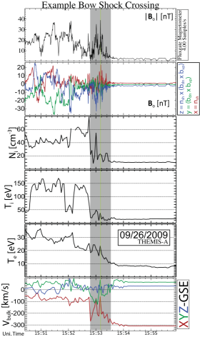
Figure 1: This figure shows a $\sim$330 s window centered on $\sim$15:53:10.080 UT (green vertical line) with magnetic field and plasma parameters, observed by THEMIS-A on 2009-09-26, for a typical supercritical oblique bow shock crossing. The top two panels show $\mid$B_o$\mid$ [nT] and B_o [NCB, nT], respectively, observed with the FGM at $\sim$4 sps. The rest of the panels show, in order, N_i [cm^-3], T_i [eV], T_e [eV], and V_bulk [GSE, km/s]. The gray shaded region indicates the timespan for Figure 2.

In this section we present examples of bow shock crossings and characteristic examples of the types of electromagnetic fluctuations observed.

We have examined 8 bow shock crossings with the THEMIS spacecraft. For every crossing, we have removed the secondary ion populations (see Appendix G) and electric field spikes due to photoelectron emissions and electrostatic wake effects. We filtered the electromagnetic fields above $\sim$10 Hz to remove DC-coupled quasi-static fluctuations from the EFI and SCM observations and convective electric fields from the EFI. A cursory comparison (not shown) between the electric fields observed at $\sim$128 sps and those at $\sim$8,192 sps show that the high frequency electric fields consistently dominate the low frequency components ($\delta$E $\gg$ E_o). Therefore, we did not focus on these lower frequency electric fields.

3.1 Overview and Examples

Figure 1 shows an example bow shock crossing observed on 2009-09-26 by THEMIS-A. The top two panels show the $\mid$B_o$\mid$ and its components in the normal incidence frame (NIF) coordinate basis (NCB, see Appendix C for definition) observed by the FGM at $\sim$4 sps. The next four panels show particle velocity moments for the ions and electrons. We removed secondary ions (see Appendix G) due to shock reflection from the upstream velocity distributions prior to calculating the ion moments in Figure 1. The change in particle velocity moments in Figure 1 reflect the supercritical nature of this shock (see Tables 1 and 2). One can see that the shock causes significant plasma compression (i.e., N_i2/N_i1 $\sim$ 4), strong ion heating (T_i2/T_i1 $>$ 6), and strong electron heating (T_e2/T_e1 $\gtrsim$ 3).

The structure of this bow shock is consistent with previous observations of supercritical bow shocks. The large variability observed in $\mid$B_o$\mid$ and B_o could be explained by sudden expansions and contractions of the bow shock or non-stationary shock reformation [e.g., Krasnoselskikh et al., 2002; Lobzin et al., 2007]. The large fluctuations in B_o correlate with significant deflections in V_bulk and changes in N_i. The details of the large fluctuations in B_o are discussed further below.

Notice that the increase in T_i is slightly delayed with respect to T_e. This is partly due to our use of only the core in determining T_i (see Appendix G) and partly a real phenomena. The flow is deflected and the electrons begin to thermalize before T_i shows any significant change. Therefore, the bulk flow reduction appears to be compensated by reflected ions and electron heating. The two phenomena are not unrelated and will be discussed in greater detail later.

The gray shaded region in Figure 1 shows the time range for Figure 2. Figure 2 shows $\sim$45 s of higher time resolution ($\sim$128 sps) magnetic field data observed by the FGM instrument. The tick marks below the plot show the universal time (UT), radial distance from center of Earth (R_E), and the distance from center of shock ramp ($\sim$15:53:10.080 UT) in three units: upstream average ion inertial lengths ($\langle c/\omega{{}_{pe}}\rangle{{}_{up}}$), convected ion gyroradii ($\rho{{}_{conv}}$ $=$ U_shn/$\langle\Omega{{}_{ci}}\rangle{{}_{down}}$), and km.

Notice that the amplitudes of both $\mid$B_o$\mid$ and its components are larger than observed by the FGM at $\sim$4 sps shown in Figure 1. The comparison illustrates that the largest amplitude fluctuations are not well resolved in the $\sim$4 sps FGM data shown in Figure 1. The fluctuations in Figure 2, which occur on spatial scales much smaller than ion scales, illustrate the highly dynamic nature of the supercritical bow shock and are commonly observed in the bow shock crossings with high time resolution magnetometers. Many of these magnetic pulsations have $\delta$B/B_o $\gtrsim$ 4 and their gradient scale lengths along the shock normal vector are on electron scales. These electromagnetic fluctuations are identified as magnetosonic-whistler mode waves.

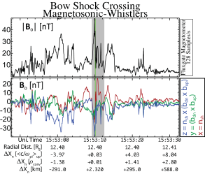
Figure 2: This figure illustrates how survey data can under-sample large amplitude fluctuations in typical bow shock crossings. It shows a $\sim$45 s window of $\mid$B_o$\mid$ and its NCB components [nT] sampled at $\sim$128 sps by the FGM. The tick marks below the plot are, from top-to-bottom, the following: (1) Time [UT], (2) radial distance from center of Earth [R_E], (3)-(5) distance from center of shock ramp in units of $\langle c/\omega{{}_{pe}}\rangle{{}_{up}}$, $\rho{{}_{conv}}$, and km. The gray shaded region indicates the timespan for Figure 3.

Nearly all of the bow shock crossings examined herein show large amplitude compressive magnetic fluctuations upstream of the shock ramp consistent with magnetosonic-whistler precursors [e.g., Wilson III et al., 2009, and references therein]. These fluctuations show enhanced power for f_ci $<$ f_sc $\lesssim$ f_lh, where f_sc is the spacecraft frame frequency. They are right-hand polarized (with respect to B_o) electromagnetic compressive fluctuations with magnetic fluctuations in phase with density fluctuations. Theory suggests that they are driven by dispersion [e.g., Kennel et al., 1985; Krasnoselskikh et al., 2002] and/or reflected ions [e.g., Wu et al., 1983; Riquelme and Spitkovsky, 2011; Comişel et al., 2011]. Observations have shown evidence to support both dispersion [e.g., Sundkvist et al., 2012] and instabilities [e.g., Wilson III et al., 2012] as the source of these waves. At highly oblique angles, these waves stochastically accelerate electrons parallel to B_o and heat ions perpendicular to B_o [e.g., Wu et al., 1983; Cairns and McMillan, 2005], which has been supported by observations [e.g., Wilson III et al., 2012].

Magnetosonic-whistlers are primarily observed with the FGM instrument because we filter the SCM data to $\geq$10 Hz to match the EFI data when AC-coupled. Figure 2 shows that these fluctuations can have amplitudes $\sim$2-4 times the upstream average field strength. Such large amplitude fluctuations raise doubts about the capacity for electrons to remain magnetized as they move through this region [e.g., Mozer and Sundkvist, 2013; Sundkvist and Mozer, 2013]. These fluctuations are rarely observed in the filtered SCM data shown herein and they are not the focus of this study.

The gray shaded region in Figure 2 shows the $\sim$3.3 s window for the time range in Figure 3. Figure 3 shows examples of the electromagnetic fluctuations that are the focus of this paper. The top two panels show the $\mid$B_o$\mid$ and its NCB components (see Appendix C for definition) observed by the FGM at $\sim$128 sps. The third and fourth panels shows $\delta$E and $\delta$B, respectively, in the spacecraft frame (SCF) of reference and in a field-aligned coordinates (FACs) basis (definition found in the inset box). Both are sampled at $\sim$8192 sps with a soft high-pass filter above $\sim$10 Hz. The fifth panel shows $\mid$$\delta\tilde{\textbf{S}}$$\mid$ (see Appendix A for definition). The 6th panel shows two components of of the current density, j_o, in NCB (see Appendix C for definition). The seventh panel shows the amount of ohmic dissipation, or $\left(-\textbf{j}{{}_{o}}\cdot\delta\textbf{E}\right)$, at the $\delta$E time steps (red) with corresponding trend line (cyan). $\delta$E was transformed into the NIF and rotated into the NCB prior to projecting onto j_o. We will discuss this figure in more detail below.

3.2 Separation of Frequencies

In this section we discuss the differences between the fluctuations in $\delta$B and $\delta$E and their dependence upon frequency. First we discuss the lower frequency magnetosonic-whistlers and then we will discuss the higher frequency electrostatic and electromagnetic modes that are the focus of this work. We discuss these two separate frequency and spatial scales within the context of their relative contributions to the energy dissipation due to the work done on the particles by the electromagnetic fields, $\left(-\textbf{j}\cdot\textbf{E}\right)$.

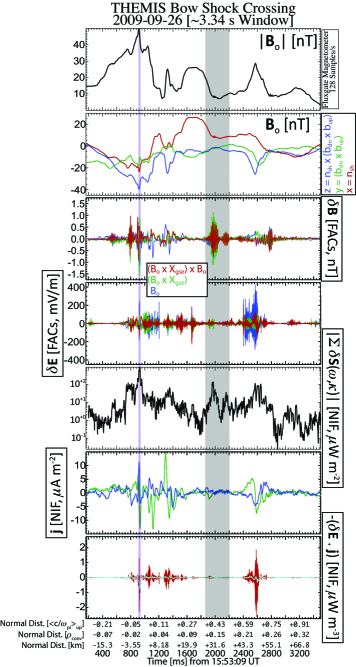
Figure 3: A $\sim$3.3 s window showing an example of the energy budget in a typical bow shock crossing. The panels are, from top-to-bottom, the following: (1) $\mid$B_o$\mid$ [nT]; (2) B_o [NCB, nT]; (3) $\delta$B [FACs, nT]; (4) $\delta$E [FACs, mV/m]; (5) $\mid$$\delta\tilde{\textbf{S}}$$\mid$ [NIF, $\mu$W m^-2]; (6) j_o [NCB, $\mu$A m^-2]; and (7) $\left(-\textbf{j}{{}_{o}}\cdot\delta\textbf{E}\right)$ [NCB, $\mu$W m^-3]. The gray shaded region shows the timespan for the example whistler mode wave shown in Figure 6. The magenta shaded region shows the timespan for the example electrostatic solitary waves shown in Figure 7.

For magnetosonic-whistlers, the largest values of E_o and B_o occur with spacecraft frame frequencies (f_sc) between the ion cyclotron (f_ci) and lower hybrid resonance (f_lh) frequencies or f_ci $<$ f_sc $\lesssim$ f_lh, which is $\sim$0.01-10 Hz for typical solar wind conditions. These fluctuations can be as large as B_o $\gtrsim$ 30 nT and E_o $\gtrsim$ 40 mV/m, but they are typically smaller with B_o $\sim$ 1-10 nT and E_o $\sim$ 5-20 mV/m. Magnetosonic-whistlers also typically have smaller S_o contributions than the higher frequency waves because they have much smaller electric fields, or E_o $\ll$ $\delta$E.

Notice in Figure 3 that the energy dissipation due to the work done on the particles by the electromagnetic fields or $\left(-\textbf{j}{{}_{o}}\cdot\delta\textbf{E}\right)$ has peak magnitudes near the sharpest gradients in B_o or the largest values of j_o. These large j_o are typically due to magnetosonic-whistlers and are typically dominated by frequencies $\lesssim$10 Hz. However, the contribution to $\left\lvert\textbf{j}\cdot\textbf{E}\right\rvert$ by magnetosonic-whistlers tends to be at least an order of magnitude smaller than the higher frequency waves (discussed below) due to their smaller $\delta$E. The peaks in $\left(-\textbf{j}{{}_{o}}\cdot\delta\textbf{E}\right)$ near these large gradients are due to the higher frequency waves. Previous observations have shown that higher frequency electromagnetic [e.g., Hull et al., 2012; Wilson III et al., 2013a] and electrostatic [e.g., Wilson III et al., 2007] fluctuations occur simultaneously with large amplitude magnetosonic-whistler precursor waves. We also find from our THEMIS observations that these higher frequency fluctuations tend to occur simultaneously with large amplitude magnetosonic-whistlers.

The occurrence of higher frequency waves near the largest values of j_o is consistent with the idea that current-driven instabilities are responsible for dissipating the necessary energy to regulate the nonlinear steepening of an electromagnetic wave [e.g., Sagdeev, 1966; Gary, 1981; Bale et al., 2005; Treumann, 2009]. Magnetosonic-whistlers are also capable of accelerating and reflecting particles when nonlinear and steepened [e.g., Wilson III et al., 2013b]. Therefore, we believe they provide an important source of free energy for the higher frequency waves (the focus of this study) and they can act as a conduit for energy/momentum exchange between fields and particles.

The data shown in Figure 3 are not unusual for bow shock crossings. Every bow shock crossing we have examined with available waveform data from Wind, STEREO, or THEMIS shows high frequency ($\gtrsim$10 Hz) large amplitude fluctuations in both $\delta$B and $\delta$E. These higher frequency waves are composed of two categories: (1) electromagnetic fluctuations; and (2) electrostatic (i.e., $\left(\textbf{k}\times\delta\textbf{E}\right)$ $\sim$ 0) fluctuations.

The high frequency waves dominated by electromagnetic components show peak values of $\delta$B between f_lh and the electron cyclotron frequency, f_ce, or f_lh $\ll$ f_sc $\leq$ f_ce. These fluctuations can have large amplitudes with $\delta$B and $\delta$E up to $\sim$2 nT and $\sim$30 mV/m, respectively, but they typically have $\delta$B $\lesssim$ 0.5 nT and $\delta$E $\lesssim$ 10 mV/m. They can produce significant contributions to $\delta$S but their contributions to $\left\lvert\textbf{j}{{}_{o}}\cdot\delta\textbf{E}\right\rvert$ tend to be small compared to the electrostatic fluctuations discussed below and they are observed less often. We also note that though these high frequency electromagnetic fluctuations can have large $\delta$B, they are always smaller than the lower frequency magnetosonic-whistlers. Thus, as one would expect, the magnetic field spectrum shows a decreasing trend with increasing frequency.

The electric fields, however, can show an inverted spectrum in the presence of high frequency electrostatic waves. Ignoring the high frequency electromagnetic fluctuations, there is typically a large frequency gap between the low frequency magnetosonic-whistlers and the higher frequency electrostatic waves. Their peak values of $\delta$E typically occur between the ion (f_pi) and electron plasma frequency (f_pe), or f_pi $\leq$ f_sc $\lesssim$ f_pe. These fluctuations have the largest contribution to $\delta$E and dominate the entire power spectrum. They can have amplitudes $\delta$E $\gtrsim$ 300 mV/m, but they typically have $\delta$E $\sim$ 10-50 mV/m. These electrostatic fluctuations typically produce the largest contributions to $\delta$S and $\left\lvert\textbf{j}{{}_{o}}\cdot\delta\textbf{E}\right\rvert$ because of their incredibly large $\delta$E.

We discuss both the high frequency electromagnetic and electric fluctuations in more detail in Section 3.3 and Appendix B.

3.3 High Frequency Waves

In this section, first we will introduce and discuss the various high frequency wave types observed. We leave the detailed examples and discussion of these high frequency waves to the appendices, which are outlined as follows: in Appendix B.1 we present some example waveforms observed by THEMIS and discuss their relevance; in Appendix B.2 we summarize the statistics of the wave properties for all high frequency waves observed by THEMIS; and finally in Appendix B.3 we show example waveforms observed by the Wind and STEREO spacecraft for comparison.

All of the bow shock crossings examined had large amplitude fluctuations in $\delta$B and $\delta$E. Nearly all of the bow shock crossings examined herein show any combination of the following electromagnetic and electrostatic fluctuations, in no particular order: (1) magnetosonic-whistler precursors [e.g., Wilson III et al., 2009, and references therein]; (2) high frequency whistler mode waves [e.g., Hull et al., 2012; Wilson III et al., 2013a]; (3) trains of electrostatic solitary waves (ESWs) or electron phase space holes [e.g., Bale et al., 1998, 2002]; (4) ion-acoustic waves (IAWs) [e.g., Wilson III et al., 2007]; and/or (5) nonlinear electrostatic fluctuations consistent with those examined by Hull et al. [2006] and Wilson III et al. [2010]. Though magnetosonic-whistlers are large and have been shown to be important [e.g., Sundkvist et al., 2012; Wilson III et al., 2012], we will not focus on them herein.

In Section 3.2, we discussed some properties of high frequency electromagnetic and electrostatic fluctuations. The high frequency electromagnetic waves are whistler mode waves. The high frequency electrostatic waves are composed of combinations of ECDI, IAWs, and trains of ESWs. As we previously discussed, the electrostatic fluctuations produce the largest contributions to $\delta$S and $\left\lvert\textbf{j}{{}_{o}}\cdot\delta\textbf{E}\right\rvert$. This is significant because theory predicts that these high frequency electrostatic waves can provide the dominant form of energy dissipation for collisionless shocks [e.g., Sagdeev, 1966; Coroniti, 1970; Tidman and Krall, 1971; Wu et al., 1984; Treumann, 2009]. In the following, we discuss recent simulation results that are consistent with our observations and conclusions.

ECDI, IAWs, and trains of ESWs (similar to those shown in Figures 5-7) are observed in nearly every bow shock crossing we have examined with not only THEMIS, but Wind [e.g., Wilson III, 2010] and STEREO [e.g., Breneman et al., 2011] as well (see Appendix B). The amplitude of these fluctuations range from $\sim$10’s of mV/m to $>$300 mV/m. These modes are observed semi-continuously from the foot through the magnetosheath. This is in contrast with some simulations which only show waves near the front(upstream) edge of the foot or shock ramp [e.g., Matsukiyo and Scholer, 2006]. However, Muschietti and Lembège [2013] noted that because these simulations (and theirs) were performed in the electron rest frame, the waves were limited to the shock foot. If the effects of convection were included, they suggest that the waves could exist everywhere in the shock transition region, consistent with our observations.

The study by Muschietti and Lembège [2013] focused on the effects of the ECDI in a perpendicular shock. We have shown that the waves predominantly observed include the ECDI as well as IAWs and ESWs. While we observed ECDI in each crossing, the majority of the electrostatic waves were more consistent with IAWs and ESWs. Muschietti and Lembège [2013] ran an example simulation to compare the evolution of the ECDI and IAWs. They found that at late times in their simulations, the ECDI and IAWs had very similar power spectrums (ignoring the peaks due to the Bernstein modes in the ECDI). The only differences were in the wave polarization and their respective effects on the particle distributions. The IAWs in their simulation began to form electron phase space holes at later times.

The similarity in the power spectrums for the ECDI and IAWs found by Muschietti and Lembège [2013] should be expected since the ECDI is a series of electron Bernstein modes coupled to Dopler-shifted IAWs. However, it adds difficulty to the unique identification of each mode. Moreover, Muschietti and Lembège [2013] found that the higher harmonics damped out leaving only the fundamental after sufficient time. The result was a well defined peak near f_ce and a broad, weaker spectrum at higher frequencies. At this point, the ECDI power spectrum looks very similar to the IAW power spectrum. Thus, it is not surprising that we identify fluctuations consistent with both the ECDI and IAWs.

As previously shown, ESWs can either couple to, or directly cause, the growth of IAWs [e.g., Dyrud and Oppenheim, 2006] or whistler mode waves [e.g., Lu et al., 2008]. Both of these modes may also be indirectly driven unstable by the large amplitude magnetosonic-whistler waves observed throughout the transition region. The large magnetic fluctuations due magnetosonic-whistlers can produce strong localized currents that can excite current-driven instabilities like IAWs. Magnetosonic-whistlers can also compress the plasma to produce a temperature anisotropy instability that may explain the origin of the high frequency whistler mode waves. Therefore, our THEMIS, Wind, and STEREO observations of combinations of ECDI, ESWs, and IAWs throughout the entire shock transition region (from foot through the magnetosheath) are consistent with simulations [e.g., Muschietti and Lembège, 2013] and previous observations [e.g., Wilson III et al., 2007, 2010, 2013a].

4 Energy Dissipation

In this section, we will show conclusive evidence that wave-particle interactions can provide enough energy dissipation to balance the nonlinear wave steepening producing the shock.

We have examined 8 bow shock crossings with the THEMIS spacecraft, where the shock parameters can be seen in Tables 1 and 2. In every THEMIS event examined, we observed large amplitude electromagnetic and electrostatic fluctuations in and around the shock ramps, with the largest amplitudes found near the sharpest magnetic field gradients. The long duration of the THEMIS waveform captures compared to those observed by Wind and STEREO show that these fluctuations can remain enhanced for $>$10 seconds. Figures 8 and 9 support our conclusion that large amplitude electromagnetic fluctuations are an ubiquitous phenomena in the collisionless bow shock transition region. Previous studies [e.g., Wilson III et al., 2007] at interplanetary shocks came to a similar conclusion. We also note that the observation of these waves is not limited to quasi-perpendicular geometry, as seen in Table 1 and previously reported by Wilson III et al. [2007]. These results add to the mounting evidence that electromagnetic waves play an important role in the macroscopic redistribution of energy in collisionless shocks. Therefore, we decided to quantify the relative contribution of these electromagnetic waves in the global energy budget of the collisionless bow shock.

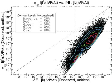
Figure 4: Plot showing that the wave energy dissipation rate often exceeds the dissipation rate necessary to produce the observed increase in entropy. The plot shows $\mathcal{Y}{{}_{\Psi}}$ ($\equiv$ $\eta{{}_{iaw}}\left\lvert\textbf{j}{{}_{o}}\right\rvert^{2}$/$\dot{\Psi}$) versus $\mathcal{R}{{}_{\Psi}}$ ($\equiv$ $\left\lvert\textbf{j}{{}_{o}}\cdot\delta\textbf{E}\right\rvert$/$\dot{\Psi}$) for all events examined herein. The contours show the percentage of points contained within each. The inset box defines the corresponding percentage.

We performed this test by calculating the ratio of the dissipation rate of the waves to the dissipation rates necessary to explain the observed increase in entropy, which we defined as $\dot{\Psi}$ $\equiv$ ($\rho$T)$\Delta\mathfrak{s}$/$\Delta$t. We calculated this ratio using two slightly different methods for reasons explained in Appendix F. The first ratio we defined as $\mathcal{Y}{{}_{\Psi}}$ $\equiv$ $\eta{{}_{iaw}}\left\lvert\textbf{j}{{}_{o}}\right\rvert^{2}$/$\dot{\Psi}$ and the second as $\mathcal{R}{{}_{\Psi}}$ $\equiv$ $\left\lvert\textbf{j}{{}_{o}}\cdot\delta\textbf{E}\right\rvert$/$\dot{\Psi}$. Physically, $\mathcal{Y}{{}_{\Psi}}$ and $\mathcal{R}{{}_{\Psi}}$ are ratios of the rate of work per unit volume done by the waves on the plasma to the rate of energy dissipation per unit volume necessary to produce the increase in entropy. Therefore, if either ratio is $\geq$ 1, then the magnitude of the rate of work per unit volume done on the particles by the fluctuating electric fields exceeds the dissipation rate necessary to produce the observed increase in entropy. Meaning, if either ratio is $\geq$ 1 then the waves can provide more than enough energy dissipation to explain the shock dynamics.

Previous observations found a high relative occurrence of IAWs in the ramp regions of interplanetary collisionless shock waves [e.g., Wilson III et al., 2007]. Therefore, we used the IAW dispersion relation to give our estimate of $\eta{{}_{iaw}}$ for $\mathcal{Y}{{}_{\Psi}}$. The assumptions used to estimate j_o are only valid near the shock ramp, so we only included wave bursts within roughly $\pm$10 seconds of the center of the shock ramp. We linearly interpolated j_o to the same time steps as $\delta$E prior to calculating $\mathcal{Y}{{}_{\Psi}}$ and $\mathcal{R}{{}_{\Psi}}$. The details of and justifications for up-sampling j_o are given in Appendix E.

Figure 4 plots $\mathcal{Y}{{}_{\Psi}}$ versus $\mathcal{R}{{}_{\Psi}}$, calculated from the high frequency waves, for all the bow shock crossings observed. The contours define regions containing a percentage of the total number of points shown, where the contour levels are defined in the inset box in the upper left-hand corner. The vertical(horizontal) dashed line shows where $\mathcal{R}{{}_{\Psi}}$($\mathcal{Y}{{}_{\Psi}}$) $=$ 1. The diagonal dashed line shows where $\mathcal{R}{{}_{\Psi}}$ $=$ $\mathcal{Y}{{}_{\Psi}}$.

In every THEMIS bow shock crossing, we found $>$100 data points (on FGM time-steps) that satisfy $\mathcal{R}{{}_{\Psi}}$ $\geq$ 1 and $\mathcal{Y}{{}_{\Psi}}$ $\geq$ 1. Note that this reduces to roughly $>$50 data points for $\mathcal{R}{{}_{\Lambda}}$ or $\mathcal{Y}{{}_{\Lambda}}$ (see Appendix F for more details). The fact that every event has $>$100 individual time steps satisfying $\mathcal{R}{{}_{\Psi}}$($\mathcal{Y}{{}_{\Psi}}$) $\geq$ 1 implies that the waves can support the global dynamics of the shock structure for at least $\sim$0.8 seconds or scale lengths ranging from $\sim$10-50 km. One can see from Figure 3 that this scale length is much larger than the typical gradient scale lengths observed in B_o and/or j_o. In addition, an examination of the DC-coupled electric field measurements (sampled at $\sim$128 sps) shows that their contribution to the wave energy dissipation, $\left\lvert\textbf{j}{{}_{o}}\cdot\textbf{E}{{}_{o}}\right\rvert$, was typically an order of magnitude lower than from the higher frequency AC-coupled measurements. Therefore, we argue that the waves have the capacity to dominate the global energy budget of collisionless shock waves.

The comparison between $\mathcal{R}{{}_{\Psi}}$ and $\mathcal{Y}{{}_{\Psi}}$ in Figure 4 shows that the our assumption $\delta$E $\approx$ $\left(\overleftrightarrow{\mathbb{\eta}}{{}_{{}_{iaw}}}\cdot\thickspace\textbf{j}{{}_{o}}\right)$ for $\mathcal{Y}{{}_{\Psi}}$ is too small by up to four orders of magnitude. This agrees with a similar comparison found in Vlasov simulations [e.g., Petkaki et al., 2006; Petkaki and Freeman, 2008; Yoon and Lui, 2006, 2007], where the analytical estimates for $\eta{{}_{iaw}}$ were found to be up to 2-3 orders of magnitude too small. Even so, this plot shows that every shock crossing has multiple points with $\mathcal{Y}{{}_{\Psi}}$ $\geq$ 1. Therefore, $\eta{{}_{iaw}}\left\lvert\textbf{j}{{}_{o}}\right\rvert^{2}$ can be used as a lower bound for an estimate of the wave energy dissipation rate in a collisionless shock.

5 Discussion

We present the first quantified measure of the energy dissipation rate, due to wave-particle interactions, in collisionless shocks. The work presented herein can be summarized by the following points:

1. Every bow shock crossing examined with available wave burst data from THEMIS showed large amplitude $\delta$E and $\delta$B high frequency ($\gtrsim$10 Hz) waves throughout the entire transition region and into the magnetosheath. These high frequency ($\gtrsim$10 Hz) wave amplitudes can exceed $\delta$B $\sim$ 10 nT and $\delta$E $\sim$ 300 mV/m, though they are typically observed at $\delta$B $\sim$ 0.1-1.0 nT and $\delta$E $\sim$ 10-50 mV/m.

2. The high frequency ($\gtrsim$10 Hz) waves were composed of multiple modes, identified as ion-acoustic waves (IAWs), electron cyclotron drift instability (ECDI), trains of electrostatic solitary waves (ESWs), and electromagnetic whistler mode waves. The low frequency ($<$10 Hz) observations were dominated by magnetosonic-whistler waves.

3. The high frequency ($\gtrsim$10 Hz) waves were found to have $\mid$$\delta\textbf{S}$$\mid$ in excess of 2000 $\mu$W m^-2, though typical values were between $\sim$ 1-10 $\mu$W m^-2. They could produce resistivities $\eta{{}_{iaw}}$ $>$ 9000 $\Omega$ m and energy dissipation rates $\left\lvert\textbf{j}{{}_{o}}\cdot\delta\textbf{E}\right\rvert$ $>$ 3 $\mu$W m^-3.

4. The cursory examination of Wind and STEREO bow shock crossings showed similar wave modes and comparable electric field amplitudes. Both spacecraft observe large amplitude ($\delta$E $\geq$ 100 mV/m) waves throughout the shock transition region and magnetosheath when ever wave burst data was available. Thus, we conclude that these large amplitude waves are ubiquitous throughout the entire shock transition region and the magnetosheath.

5. The low frequency ($<$10 Hz) magnetosonic-whistler waves were also an ubiquitous mode upstream of the shock ramps, but we did not focus on them. While their magnetic amplitudes can be very large (B_o $>$ 30 nT), their contribution to the wave energy dissipation was typically an order of magnitude less than from the higher frequency modes, or $\left\lvert\textbf{j}{{}_{o}}\cdot\textbf{E}{{}_{o}}\right\rvert$ $\ll$ $\left\lvert\textbf{j}{{}_{o}}\cdot\delta\textbf{E}\right\rvert$.

6. When we compared the wave energy dissipation rates, $\left\lvert\textbf{j}{{}_{o}}\cdot\delta\textbf{E}\right\rvert$ and $\eta{{}_{iaw}}\left\lvert\textbf{j}{{}_{o}}\right\rvert^{2}$, to the values necessary to produce the observed increase in entropy, $\dot{\Psi}$ ($\equiv$ $\rho T\Delta\mathfrak{s}/\Delta t$), we found that every event has a majority of data points where $\mathcal{R}{{}_{\Psi}}$ ($\equiv$ $\left\lvert\textbf{j}{{}_{o}}\cdot\delta\textbf{E}\right\rvert$/$\dot{\Psi}$) $>$ 1 or $\mathcal{Y}{{}_{\Psi}}$ ($\equiv$ $\eta{{}_{iaw}}\left\lvert\textbf{j}{{}_{o}}\right\rvert^{2}$/$\dot{\Psi}$) $>$ 1. Moreover, the wave dissipation rates can greatly exceed the dissipation rates necessary to balance the nonlinear steepening of the shock ramp. These results have the following implications:

   1. The waves can provide more than enough energy dissipation to produce the observed increase in entropy across the shock ramp.

   2. Therefore, the waves can provide enough energy dissipation to balance the nonlinear wave steepening leading to the shock itself.

   3. More importantly, this implies that the efficiency of the wave energy dissipation need only be $\lesssim$ 0.01% to regulate the global shock dynamics.

7. We performed an example calculation for the growth rates of the ECDI in every event to verify that the instability could reach sufficient amplitude before convecting into the downstream. Our estimates showed that the waves could saturate in much less time than is necessary for them to convect across the shock foot alone. Therefore, we can conclude that the waves can be driven by an instability upstream of the shock ramp and still provide sufficient energy dissipation before convecting downstream.

These observations are the first results that quantitatively show that wave-particle interactions have the capacity to control the global dynamics of collisionless shock waves. These results support recent observations [e.g., Wilson III et al., 2007, 2010, 2012] and simulations [e.g., Matsukiyo and Scholer, 2006; Comişel et al., 2011; Muschietti and Lembège, 2013] that suggest microphysical processes can dominate the global structure of low Mach number collisionless shocks.

Observations with $\mathcal{R}{{}_{\Psi}}$ $>$ 1 or $\mathcal{Y}{{}_{\Psi}}$ $>$ 1 are highly suggestive of the relative importance of wave-particle-driven energy dissipation. The physical significance of observing $\mathcal{R}{{}_{\Psi}}$ $\geq$ 1 or $\mathcal{Y}{{}_{\Psi}}$ $\geq$ 1 implies that the waves are capable of providing more energy dissipation than is necessary to produce the observed increase in entropy. This means that there is more work done by the wave electric fields on the particles in a unit volume than is necessary to balance the nonlinear wave steepening that leads to the shock formation. More importantly, this implies that the waves need not be 100% efficient when exchanging energy/moment with the particles to explain the observed increase in entropy. In fact, the data corresponding to $\mathcal{R}{{}_{\Psi}}$ in Figure 4 show that the electromagnetic fluctuations need only be, at times, $<$ 0.01% efficient to mediate the global shock transition.

We emphasize the efficiency of the wave dissipation because we observe two other energy loss mechanisms in many of these shock waves. For instance, all the THEMIS events satisfy M_f/M_cr $>$ 1 (i.e., supercritical), implying ion reflection, which we observe in the analyzed shocks. In addition, many of the THEMIS shock crossings observed have magnetosonic-whistler precursors, which can carry energy away from the shock ramp. Therefore, at least some of the incident bulk flow kinetic energy may be lost through mechanisms other than wave-particle interactions. Note that reflection is not, alone, an irreversible process. However, we have quantitatively shown that these high frequency waves have the capacity to be the dominant energy dissipation mechanism.

While particle reflection can be an energy loss mechanisms that collisionless shock waves use to balance nonlinear wave steepening, it cannot transform the incident bulk flow kinetic energy into thermal energy irreversibly through direct means. For instance, if the reflected ions drive an instability that then stochastically scatters incident particles, then they can indirectly transform energy irreversibly through the instability. As discussed in Section 3.3, we believe the observed high frequency waves are driven by unstable particle distributions. The most likely source of free energy for many of the observed modes is due to the relative drift between the reflected ions and incident electrons and/or ions.

We now discuss whether the dispersive radiation of a magnetosonic-whistler precursor wave, due to nonlinear wave steepening, is an irreversible process. The dispersive properties of magnetosonic-whistler waves result in the higher(smaller) frequency(wavelength) propagating faster than the lower frequencies. Therefore, the shock ramp can appear to be a train of compressive magnetosonic-whistler waves with the highest frequency waves observed the farthest from the shock ramp. One might think that the spatial spreading of frequency components is not directly irreversible. However, one does not expect a radiated wave to return to its source without external influences. In addition, if the radiated waves carry momentum/energy into the upstream (i.e., their group velocity exceeds the shock velocity), then they are directly removing momentum/energy from the shock. Thus, until the radiated waves interact with the upstream medium and impart their momentum/energy to the plasma, it is not immediately obvious that this process is directly irreversible.

If these waves are dispersively radiated and they carry energy away from the shock ramp, then they can indirectly transform energy (irreversibly) by either stochastically scattering particles directly or exciting waves that scatter the particles. In the latter case, their large magnetic fluctuations can produce strong localized currents that drive electrostatic instabilities (e.g., IAWs) or they can compress the plasma to produce temperature anisotropy instabilities (e.g., whistler mode waves). Previous observations have found that higher frequency electrostatic [e.g., Wilson III et al., 2007] and electromagnetic [e.g., Hull et al., 2012; Wilson III et al., 2013a] waves occur simultaneously with large amplitude magnetosonic-whistler waves. Note that previous studies have found that the magnetosonic-whistlers can be generated either by dispersion [e.g., Sundkvist et al., 2012] or instabilities [e.g., Wilson III et al., 2012].

Note that in both of these scenarios, particle reflection or dispersive radiation, the end state is an irreversible transformation of energy at a microscopic scale through wave-particle interactions. Whether the high frequency waves we observe throughout the transition region were driven by the free energy from the reflected ions or by the localized currents in the magnetosonic-whistlers is not the focus of this study. The over abundance of potential energy dissipation that these high frequency waves can produce is the most important result in our study. Theory and simulation have shown that the observed modes are capable of efficiently exchanging energy/momentum between particle species leading to an irreversible transformation of energy.

Therefore, we conclude that the observed wave modes have the capacity to dominate the global dynamics of collisionless shock waves.

Acknowledgements
We would like to thank A.F.- Viñas, D. Sundkvist, V.V. Krasnoselskikh, D. Bryant, D.A. Roberts, R. Lysak, and M.L. Goldstein for useful discussions of the fundamental physics involved in our study.

References

Appendix A Analysis Techniques

In this appendix we outline some of our analysis techniques.

For events where the EFI was sampling at $\sim$16,384 sps while the SCM was sampling at $\sim$8,192 sps, we down-sampled the EFI to the SCM time steps, after calibration. Then these two fields, $\delta$E and $\delta$B, were used to estimate the Poynting flux, $\delta$S [$=$ ($\delta$E$\times\delta$B)/$\mu{{}_{o}}$], in temporal and frequency space. $\delta$S was calculated after both $\delta$E and $\delta$B were filtered and after each was transformed or rotated into the desired reference frame or coordinate basis, respectively.

The frequency space estimate, $\mid$$\delta\tilde{\textbf{S}}$$\mid$, involves summing over the Fourier transformed time and frequency bins of $\delta$S to estimate the magnitude of the electromagnetic energy flux. We calculated $\mid$$\delta\tilde{\textbf{S}}$$\mid$ through the following steps: (1) create a Hanning window with N_fft elements and multiply by $\delta$B_i:k and $\delta$E_i:k, i.e., where $i$ and $k$ are the first and last abscissa of any given N_fft-element increment; (2) calculate the Fourier transform (FFT) of these products, $\delta\tilde{\textbf{E}}{{}_{i:k}}$ and $\delta\tilde{\textbf{B}}{{}_{i:k}}$, respectively; (3) calculate $\delta\tilde{\mathfrak{P}}{{}_{i:k}}$ $=$ $\delta\tilde{\textbf{E}}{{}_{i:k}}\times\delta\tilde{\textbf{B}}{{}_{i:k}}^{*}$/(2$\mu{{}_{o}}$) in frequency space; (4) calculate $\delta\tilde{\mathfrak{S}}{{}_{m}}^{2}$ $=$ $\sum_{i}^{k}$ $\mid$$\delta\tilde{\mathfrak{P}}{{}_{i:k}}$$\mid^{2}$; and (5) finally, $\mid$$\delta\tilde{\textbf{S}}$$\mid$ $=$ $\delta\tilde{\mathfrak{S}}{{}_{m}}$ $\Delta$f, where $\Delta$f is the bandwidth for any given N_fft-element increment.

The purpose of calculating $\mid$$\delta\tilde{\textbf{S}}$$\mid$ was to examine the upper bound on $\delta$S. This calculation decomposes the signal into frequency space before performing the cross-product, which ensures that matching frequency components were multiplied together. However, $\mid$$\delta\tilde{\textbf{S}}$$\mid$ will return positive definite values even if $\delta$S is periodically varying.

Before moving on, we will explain the uncertainties shown in Table 1. For each shock crossing, we selected a time range for the upstream and downstream regions with an equal number, $N$, of particle moment time-steps, t_i. The time ranges were selected “by-eye” and were chosen by attempting to minimize changes in the particle velocity moments and magnetic field vectors to the Rankine-Hugoniot relations. The Rankine-Hugoniot relations are numerically minimized for each input set of particle velocity moments and magnetic field vectors, Y_ij, where $i$ is the abscissa for the time-steps and $j$ defines the plasma parameter (e.g., number density). The uncertainties for V_shn and U_shn depend upon $N$ and tend to decrease with increasing $N$. Therefore the uncertainties for V_shn and U_shn are given by the standard deviation of the mean or $\sigma{{}_{x}}/\sqrt{N}$. The rest of the parameter uncertainties are given by the standard deviation or $\sigma{{}_{x}}$.

Table 2: Critical Mach Number Ratios

Date	Mf/Mcr	Mf/Mw	Mf/Mgr	Mf/Mnw
2009-07-13 [1st Crossing]	2.97 $\pm$ 0.10	0.20 $\pm$ 0.02	0.15 $\pm$ 0.01	0.14 $\pm$ 0.01
2009-07-21 [1st Crossing]	1.45 $\pm$ 0.13	0.15 $\pm$ 0.02	0.12 $\pm$ 0.01	0.11 $\pm$ 0.01
2009-07-23 [1st Crossing]	2.50 $\pm$ 0.06	1.24 $\pm$ 0.48	0.95 $\pm$ 0.37	0.88 $\pm$ 0.34
2009-07-23 [2nd Crossing]	2.98 $\pm$ 0.07	5.24 $\pm$ 5.19	4.04 $\pm$ 4.00	3.71 $\pm$ 3.67
2009-07-23 [3rd Crossing]	2.61 $\pm$ 0.07	0.25 $\pm$ 0.02	0.19 $\pm$ 0.02	0.18 $\pm$ 0.02
2009-09-26 [1st Crossing]	4.61 $\pm$ 0.26	0.45 $\pm$ 0.13	0.35 $\pm$ 0.10	0.32 $\pm$ 0.09
2011-10-24 [1st Crossing]	2.02 $\pm$ 0.04	1.00 $\pm$ 0.75	0.77 $\pm$ 0.58	0.71 $\pm$ 0.53
2011-10-24 [2nd Crossing]	1.75 $\pm$ 0.01	2.58 $\pm$ 1.48	1.99 $\pm$ 1.14	1.83 $\pm$ 1.05

We have examined 8 bow shock crossings so far. For each crossing, we calculated M_f and then determined whether the shock was supercritical or not. The first critical Mach number, M_cr, determines the theoretical value of M_f, above which, the shock can no longer dissipate sufficient energy using resistivity or dispersion alone [Edmiston and Kennel, 1984]. There are three whistler critical Mach numbers [Krasnoselskikh et al., 2002] and are defined as: M_w corresponds to the maximum Mach number at which a linear whistler can phase stand with respect to the shock front; M_gr is the maximum Mach number which would allow a whistler wave to carry energy into the upstream; and M_nw is the maximum Mach number for which a stationary shock front solution can be found, above which, the wave breaks. The Mach ratios can be seen in Table 2.

The values shown in Table 2 were calculated using the Y_ij inputs. We calculated each Mach number with associated standard deviations, giving us M_k $\pm$ $\sigma{{}_{k}}$. We then calculated the ratio of M_f to each of the critical Mach numbers discussed above and used the standard technique for the propagation of uncertainties [i.e., $\delta$q/$\mid$q$\mid$ $=$ (($\delta$x/x)² $+$ … $+$ ($\delta$z/z)²)^1/2, where q $=$ q(x,…,z)]. As one can see, every shock examined herein satisfies M_f/M_cr $>$ 1, and is therefore supercritical.

From Poynting’s theorem (see Appendix F, Equation F.2), we can see that $\left\lvert\textbf{j}\cdot\textbf{E}\right\rvert$ ($\sim$ $\left\lvert\textbf{j}{{}_{o}}\cdot\delta\textbf{E}\right\rvert$) is an energy sink/loss (see Appendix E for estimation of j_o), called ohmic dissipation. Therefore, we will use this as our first estimate of wave energy dissipation. After some assumptions, we can rewrite this term as $\eta{{}_{iaw}}\left\lvert\textbf{j}{{}_{o}}\right\rvert^{2}$, which will be our second estimate of energy dissipation. We use two methods to estimate the wave dissipation rate because each method relies upon assumptions and each method has advantages/disadvantages (see Appendix F).

The most important analysis in this paper is our quantitative comparison between the macroscopic and wave energy (microscopic) dissipation rates. To do this, we calculated the ratio of the wave energy dissipation rate to the energy dissipation rate necessary to produce the observed increase in specific entropy density per unit time, or ($\rho$T)$\Delta\mathfrak{s}$/$\Delta$t ($\equiv$ $\dot{\Psi}$). These ratios, $\mathcal{Y}{{}_{\Psi}}$ $\equiv$ $\eta{{}_{iaw}}\left\lvert\textbf{j}{{}_{o}}\right\rvert^{2}$/$\dot{\Psi}$ and $\mathcal{R}{{}_{\Psi}}$ $\equiv$ $\left\lvert\textbf{j}{{}_{o}}\cdot\delta\textbf{E}\right\rvert$/$\dot{\Psi}$, were calculated to estimate the wave energy (microscopic) dissipation rate (see Equations F.4a and F.4b) relative to the macroscopic energy dissipation rate.

Though we did examine the low frequency ($\leq$10 Hz) fields, we found that they consistently showed E_o $\ll$ $\delta$E and $\left\lvert\textbf{j}{{}_{o}}\cdot\textbf{E}{{}_{o}}\right\rvert$ $\ll$ $\left\lvert\textbf{j}{{}_{o}}\cdot\delta\textbf{E}\right\rvert$. Therefore, we have assumed that the ratios $\mathcal{Y}{{}_{\Psi}}$ and $\mathcal{R}{{}_{\Psi}}$ are dominated by the high frequency ($\gtrsim$10 Hz) waves that we focus on in this study.

Appendix B High Frequency Wave Observations

B.1 THEMIS Waves: Examples

The first instability we will discuss involves the nonlinear electrostatic fluctuations. We will then discuss observations of ESWs, high frequency whistler mode waves, and finally ion-acoustic waves (IAWs).

Figure 5: An example of an ECDI waveform and corresponding wavelet transforms observed by the EFI instrument in wave burst mode for a 40 ms time window near the shock ramp on 2009-07-13. The right-hand column shows the corresponding wavelet transforms [Torrence and Compo, 1998] with the frequency on a logarithmic scale from $\sim$10-4000 Hz.

Hull et al. [2006] described these nonlinear fluctuations as electrostatic IAWs while Wilson III et al. [2010] argued they were consistent with the electron cyclotron drift instability (ECDI) [e.g., Muschietti and Lembège, 2013]. The ECDI fluctuations are consistent with a mixture of Doppler shifted IAWs and electron cyclotron harmonics at integer and half-integer harmonics of f_ce. They are driven unstable by the relative drift between incident electrons and shock-reflected ions [e.g., Matsukiyo and Scholer, 2006; Muschietti and Lembège, 2013]. In this paper, we show evidence to support our hypothesis that these fluctuations are consistent with the ECDI.

Figure 5 shows an example of an ECDI waveform observed by THEMIS-B near the bow shock ramp on 2009-07-13. The left-hand column shows the three electric field components in field-aligned coordinates (FACs) with corresponding amplitudes defined by the black arrows at the right-hand side of each panel. Each wavelet is shown on the same color-scale range defined by the color bar at the bottom of the right-hand column. Overlaid on the wavelets are color-coded lines showing integer and half-integer harmonics of f_ce.

The fluctuations have waveform and frequency spectrum characteristics similar to previous observations [e.g., Hull et al., 2006; Wilson III et al., 2010]. However, this wave shows properties consistent with the ECDI-driven waves described by Wilson III et al. [2010], not simple Doppler shifted IAWs [e.g., see Figure 10 in Wilson III et al., 2010]. The shared properties include: (1) asymmetric oscillation of $\delta$E about a mean value [i.e., may imply a net potential drop]; (2) significant amplitudes perpendicular to B_o; (3) significant amplitudes parallel to the shock normal vector (not shown); and (4) power focused at integer and half-integer harmonics of f_ce.

ECDI-driven waves are important for shock physics because they are capable of resonantly interacting with the bulk of the ion distribution and preferentially heating the electrons perpendicular to B_o [Forslund et al., 1970, 1972; Lampe et al., 1972]. More recent work has shown that the ECDI can produce a suprathermal tail on the ion distribution and strongly heat the electrons [Muschietti and Lembège, 2013]. This is accomplished through the following process: (1) the ECDI is excited at multiple harmonics of f_ce by removing bulk kinetic energy from the reflected ions; (2) these electrostatic fluctuations interact with the electrons and trap some of the reflected ions; (3) the wave amplitudes decrease, where higher harmonics experience more damping than lower harmonics; thus allowing (4) the waves to exchange energy and momentum between particle species irreversibly.

Figure 6: An example of a typical high frequency whistler mode wave observed by the SCM instrument in wave burst mode for a $\sim$340 ms time window near the shock ramp on 2009-09-26 (gray shaded timespan in Figure 3). The format is similar to that of Figure 5 except that this shows three magnetic field components, the frequency ranges from $\sim$1-1000 Hz, and only f_lh and f_ce are shown.

Figure 6 shows an example of a typical high frequency (f_lh $\ll$ f $<$ f_ce) electromagnetic whistler mode wave. Previous observations of these modes found that they propagate at small angles relative to B_o [e.g., Hull et al., 2012; Wilson III et al., 2013a], as illustrated by the relatively small ratios of $\delta$B_∥/$\delta$B_⟂ in Figure 6. The waves are often observed as short duration ($\sim$few 10’s to 100’s of ms) bursty wave packets and can have large amplitudes ($\delta$B $>$ few nT). The corresponding electric field amplitudes for this example ranged from $\sim$few mV/m up to $\sim$30 mV/m.

High frequency electromagnetic whistler mode waves are commonly observed in and around the ramp region [e.g., Hull et al., 2012] and downstream [e.g., Wilson III et al., 2013a] of collisionless shocks. The source of these modes is thought to be either an electron temperature anisotropy (T_⟂/T_∥ $>$ 1) instability [e.g., Kennel and Petscheck, 1966] or an electron heat flux instability [e.g., Gary et al., 1994]. These modes are important because they are thought to regulate the electron heat flux and electron halo temperature anisotropy in the solar wind. At shocks, these modes are important because they can efficiently exchange energy/momentum between electrons and ions and can couple to multiple wave modes [Dyrud and Oppenheim, 2006].

Therefore, whistler mode waves have multiple pathways to transform energy from electromagnetic to kinetic or vice versa. Note, however, that these modes are observed less often and their contribution to $\left\lvert\textbf{j}{{}_{o}}\cdot\delta\textbf{E}\right\rvert$ is often much smaller (e.g., see Figure 3) than the electrostatic modes. This is not to say these modes are unimportant because previous studies have shown that they can have a significant influence on the halo energy electrons [e.g., Gary et al., 1994; Wilson III et al., 2013a].

Figure 7 shows an example of two large amplitude ESWs observed at the peak of the shock overshoot (see magenta region in Figure 3). The low frequency ($\lesssim$40 Hz) signal, on which the ESWs bipolar signatures are superposed, is most likely artificial and should be ignored. The fluctuations have waveform and frequency spectrum characteristics similar to previous observations of ESWs [e.g., Bale et al., 1998; Wilson III et al., 2007, 2010]. ESWs are often too short in duration for many electric field detectors to resolve. Even at $\sim$8,192 sps, these two examples are nearly under-sampled. The same fluctuations observed at $\sim$16,384 sps (not shown), by comparison, show smooth and continuous bipolar pulses in $\delta$E_∥.

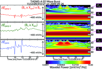
Figure 7: An example of two ESWs observed by the EFI instrument in wave burst mode for a $\sim$30 ms time window near the shock ramp on 2009-09-26 (magenta shaded timespan in Figure 3). The frequency axis of the wavelet plots range from $\sim$1-1000 Hz. The format is similar to that of Figures 5 and 6.

ESWs can be driven unstable by electron beams [e.g., Cattell et al., 2005; Ergun et al., 1998; Franz et al., 2005], modified two-stream instability (MTSI) [e.g., Matsukiyo and Scholer, 2006], etc. ESWs are one of the more important modes because they can trap incident electrons [e.g., Dyrud and Oppenheim, 2006; Lu et al., 2008], heat ions [e.g., Ergun et al., 1998], and/or couple to (or directly cause) the growth of IAWs [e.g., Dyrud and Oppenheim, 2006], whistler mode waves [Lu et al., 2008], and/or electron acoustic waves [e.g., Matsukiyo and Scholer, 2006]. Thus, solitary waves can directly heat and/or scatter particles or they can indirectly cause these effects through the generation of, or coupling to, secondary waves. Because ESWs act like clumps of positive charge, they can efficiently scatter incident ions. Previous observations have shown that a train of ESWs can increase T_⟂,i by as much as the total initial thermal energy [Ergun et al., 1998].

B.2 THEMIS Waves: Properties

In this appendix we present a summary of our statistical analysis of the wave amplitudes to help illustrate that they are important, large, and their relevance to shock physics.

From our THEMIS bow shock crossings, we have 731140 data points up-sampled to the $\delta$E time stamps (justification given in Appendix E). From those data points, we found the statistics shown in Table 3. The columns are defined in the following order: (1) parameter name and units; (2) minimum value; (3) maximum value; (4) mean or average value, $\langle$X$\rangle$; (5) standard deviation, $\sigma{{}_{x}}$; (6) standard deviation of the mean, $\sigma{{}_{x}}$/$\sqrt{N}$; and (7) the number of points used, N. In Table 3 we use the following definitions for brevity: $\mathfrak{B}$ $\equiv$ $\mid$$\delta$B$\mid$/$\langle\mid$B_o$\mid\rangle{{}_{up}}$, $\mathfrak{b}$ $\equiv$ $\mid$B_o$\mid$/$\langle\mid$B_o$\mid\rangle{{}_{up}}$, $\mathcal{W}{{}_{B}}$ $\equiv$ $\mid$$\delta$B$\mid^{2}$/(2$\mu{{}_{o}}$), $\mathcal{W}{{}_{E}}$ $\equiv$ $\varepsilon{{}_{o}}\mid$$\delta$E$\mid^{2}$/2, $\mathfrak{E}$ $\equiv$ $\mid$$\delta$E$\mid$/(c $\langle\mid$B_o$\mid\rangle{{}_{up}}$), $\mathcal{S}{{}_{\eta}}$ $\equiv$ $\eta{{}_{iaw}}\left\lvert\textbf{j}{{}_{o}}\right\rvert^{2}$, $\mathfrak{R}{{}_{\eta}}$ $\equiv$ $\left\lvert\textbf{j}{{}_{o}}\cdot\delta\textbf{E}\right\rvert$, $\mathcal{R}{{}_{\Psi}}$ $\equiv$ $\left\lvert\textbf{j}{{}_{o}}\cdot\delta\textbf{E}\right\rvert$/$\dot{\Psi}$, and $\mathcal{Y}{{}_{\Psi}}$ $\equiv$ $\eta{{}_{iaw}}\left\lvert\textbf{j}{{}_{o}}\right\rvert^{2}$/$\dot{\Psi}$ (defined in Appendix F).

Table 3: Wave Property Statistics

Type	Min.	Max.	$\langle$X$\rangle$	$\sigma{{}_{x}}$	$\sigma{{}_{x}}$/$\sqrt{N}$	N
$\mid$$\delta$E$\mid$ [mV m-1]	4.16$\times$10-02	2.99$\times$10+02	1.34$\times$10+01	1.85$\times$10+01	2.16$\times$10-02	730855
$\mid$$\delta$B$\mid$ [nT]	5.60$\times$10-04	1.00$\times$10+01	2.53$\times$10-01	4.53$\times$10-01	5.30$\times$10-04	731136
$\mid$$\delta$S$\mid$ [$\mu$W m-2]	4.93$\times$10-05	2.08$\times$10+03	3.13$\times$10+00	1.54$\times$10+01	1.80$\times$10-02	730812
$\mid$$\delta\tilde{\textbf{S}}$$\mid$ [$\mu$W m-2]	7.26$\times$10-03	2.89$\times$10+03	1.95$\times$10+01	7.65$\times$10+01	8.96$\times$10-02	728047
$\mathfrak{B}$ [unitless]	4.74$\times$10-05	1.45$\times$10+00	2.77$\times$10-02	4.18$\times$10-02	4.88$\times$10-05	731136
$\mathfrak{b}$ [unitless]	1.92$\times$10-01	1.64$\times$10+01	3.70$\times$10+00	1.62$\times$10+00	1.89$\times$10-03	731140
$\mathfrak{E}$ [unitless]	3.66$\times$10-05	3.29$\times$10-01	7.06$\times$10-03	1.29$\times$10-02	1.51$\times$10-05	730855
$\mathcal{W}{{}_{B}}$ [$\mu$W m-3]	1.25$\times$10-13	3.99$\times$10-05	1.07$\times$10-07	6.79$\times$10-07	7.94$\times$10-10	731136
$\mathcal{W}{{}_{E}}$ [$\mu$W m-3]	7.67$\times$10-15	3.96$\times$10-07	2.31$\times$10-09	1.03$\times$10-08	1.20$\times$10-11	730855
$\nu{{}_{iaw}}$ [coll. s-1]	3.72$\times$10-05	2.48$\times$10+03	5.75$\times$10+00	3.30$\times$10+01	3.86$\times$10-02	730756
$\eta{{}_{iaw}}$ [$\Omega$ m]	6.52$\times$10-05	9.38$\times$10+03	1.67$\times$10+01	1.13$\times$10+02	1.33$\times$10-01	730756
$\mathfrak{R}{{}_{\eta}}$ [$\mu$W m-3]	2.85$\times$10-11	3.98$\times$10+00	1.41$\times$10-02	6.11$\times$10-02	7.14$\times$10-05	730855
$\mathcal{S}{{}_{\eta}}$ [$\mu$W m-3]	1.08$\times$10-15	5.15$\times$10-01	1.94$\times$10-04	4.61$\times$10-03	5.39$\times$10-06	730756
$\mathcal{Y}{{}_{\Psi}}$ [unitless]	2.76$\times$10-12	8.75$\times$10+03	5.99$\times$10+00	8.72$\times$10+01	1.02$\times$10-01	730756
$\mathcal{R}{{}_{\Psi}}$ [unitless]	1.10$\times$10-05	1.59$\times$10+05	8.40$\times$10+02	2.80$\times$10+03	3.27$\times$10+00	730855

One can see that there are a wide range of wave amplitudes with high frequency (i.e., AC-coupled) electric and magnetic fields exceeding 250 mV/m and 10 nT, respectively. The magnetic fluctuations relative to an upstream averaged magnetic field magnitude, $\mid$B_o$\mid$/$\langle\mid$B_o$\mid\rangle{{}_{up}}$ (FGM) can easily exceed $\sim$ 10 and $\mid$$\delta$B$\mid$/$\langle\mid$B_o$\mid\rangle{{}_{up}}$ (SCM) can exceed $\sim$ 1. The peak values for $\mid$$\delta\textbf{S}$$\mid$ and $\mid$$\delta\tilde{\textbf{S}}$$\mid$ can exceed 2000 $\mu$W m^-2. These values are incredibly large, comparable to the energy fluxes needed to drive the terrestrial aurora [e.g., Angelopoulos et al., 2002; Wygant et al., 2000] and larger than the largest values observed for whistler mode waves in the radiation belts [e.g., see example in Wilson III et al., 2011]. Such large values illustrate the relative importance of these high frequency waves in collisionless shock dissipation.

To verify that these fluctuations can indeed result from instabilities, we will show example growth rate estimates for the ECDI [e.g., see Equation 8 in Muschietti and Lembège, 2013]. We need to confirm that the waves can grow to a sufficient amplitude in less time than is necessary to convect across the shock foot. The physically significant time scale is the lower hybrid resonance period, $\tau{{}_{lh}}$ ($=$ 2$\pi$/$\omega{{}_{lh}}$, where $\omega{{}_{lh}}$ $=$ $\left(\Omega{{}_{ci}}\Omega{{}_{ce}}\right)^{1/2}$). The growth rate of the ECDI for large wavelengths is $\gamma{{}_{max}}$ $\sim$ $\left(M{{}_{i}}/m{{}_{e}}\right)^{3/4}\left(\alpha/8\pi\right)^{1/4}\Omega{{}_{ci}}$, where $\alpha$ is the ratio of ion beam to total ion density. Let us we define a convection scale length, L_conv $\equiv$ V_e$\tau{{}_{lh}}$ (where V_e is the incident electron speed in the shock frame), and a scale length for the shock foot, L_f $\equiv$ U_shn/$\langle\Omega{{}_{ci}}\rangle{{}_{up}}$. Then we can say that L_conv/L_f $<$ 1 means that the waves could grow to sufficient amplitudes before convecting across the shock foot.

For the THEMIS events examined herein, we found 0.0007 $\lesssim$ L_conv/L_f $\lesssim$ 0.14. Therefore, the waves should convect distances much less than the scale of the shock foot and thus should be observed at significant amplitudes throughout this region. As we discussed in Appendix B.1 and Appendix B.3, we observe large amplitude waves throughout the entire transition region, consistent with the simulation results of Muschietti and Lembège [2013].

B.3 Wind and STEREO Examples

Figure 8: Seven waveform captures observed by the Wind/WAVES instrument during an inbound bow shock crossing on 1996-12-02.

In this appendix we show a few waveform capture examples observed by the Wind/WAVES [Bougeret et al., 1995] and STEREO S/WAVES [Bale et al., 2008; Bougeret et al., 2008] instruments. The examples are characteristic of the observations from both spacecraft for every bow shock crossing examined by either Wind or STEREO.

Figure 8 shows a series of seven waveform captures, $\sim$17.1 ms in duration, observed by the spin-stabilized Wind spacecraft during a bow shock crossing on 1996-12-02. The electric fields are shown in instrument coordinates (non-rotating coordinates) sampled at $\sim$120,000 sps. By instrument coordinates we mean that $\delta$E_x(y) corresponds to data only from the X(Y)-antenna, $\sim$100(15) m tip-to-tip, without being rotated into a spacecraft or physically significant coordinate basis. The purpose of showing the data in this manner prevents mixing of different noise levels from the different antenna since they have very different lengths.

The columns in Figure 8 show the following: (left) $\delta$E_x; (middle) $\delta$E_y; and (right) $\delta$E_y vs. $\delta$E_x with B_o projected onto the plane (green line). The hodograms are uniformly scaled with the same range as the Y-axis range in the two left columns. The black arrows in the left-hand column gives the relative scale of $\sim$200 mV/m for each waveform. The data are shown in instrument coordinates with associated hodograms in the right-most column. The hodograms show only the central 1/9th of the data. This is to aid the reader in comparing the polarization to the projection of B_o.

Waveforms A and B in Figure 8 are consistent with trains of ESWs [e.g., Bale et al., 1998, 2002], waveform C is consistent with ECDI-driven waves [e.g., Wilson III et al., 2010], and waveforms D and G are consistent with IAWs [e.g., Wilson III et al., 2007]. One can see that every wave shown here has $\delta$E $\gtrsim$ 150 mV/m peak-to-peak. These types of waves were observed in the shock ramp and throughout the magnetosheath of every Wind event we examined. These large amplitude waves were observed in bow shock crossing when waveform capture data was available. The waves are consistent with those we observed with the THEMIS spacecraft.

Figure 9 shows an example waveform capture, $\sim$16.4 ms in duration, sampled at $\sim$250,000 sps, observed by the STEREO-Ahead spacecraft during a bow shock crossing on 2006-11-17. The data are shown in field-aligned coordinates (FACs), where the component directions are defined in the plot. The columns show, in the following order: (left) raw $\delta$E_j; (middle) corrected $\delta$E_j; and (right) $\delta$E_j vs. $\delta$E_i with the quasi-static magnetic field vector projected onto the plane (black line). The hodograms are uniformly scaled with the same range as the Y-axis range in the two left columns. One can see that the wave is polarized primarily along quasi-static magnetic field.

Figure 9: An example waveform capture observed by the STEREO S/WAVES instrument during a bow shock crossing on 2006-11-17.

These fluctuations are consistent with a train of ESWs. The typical waveforms observed by STEREO [e.g., Breneman et al., 2011] are similar to those observed by Wind and those observed by THEMIS. Again, in every bow shock crossing we examined with available waveform data, we observed waves with $\delta$E $\gtrsim$ 150 mV/m peak-to-peak.

Therefore, we conclude that large amplitude electrostatic waves are an ubiquitous phenomena in the Earth’s collisionless bow shock. The observations by Wind and STEREO add to the evidence supplied by our THEMIS observations that high frequency waves play an important role in the global energy dissipation budget of medium Mach number ($\sim$2-6) collisionless shocks.

Appendix C Normal Incidence Frame and Coordinate Basis

C.1 Normal Incidence Frame

In this appendix, we will define our reference frame transformation into the Normal Incidence Frame (NIF) and coordinate basis rotations into the Normal incidence frame Coordinate Basis (NCB). We will present the transformations/rotations in a generalized manner, but for the purposes of this manuscript the measurements are in the SpaceCraft Frame (SCF) and GSE coordinate basis. We define the generalized basis as the Input Coordinate Basis (ICB).

We can define the velocity transformation from any arbitrary frame of reference (e.g. SCF) to the shock frame of reference (SHF) as:

$$\textbf{V}{{}_{sh}}^{rest}=\textbf{V}^{arb.}-\left(\textbf{V}{{}_{sh}}^{arb.}\cdot\hat{\textbf{n}}\right)\hat{\textbf{n}}$$ (C.1)

where $\hat{\textbf{n}}$ is the vector normal to the assumed planar shock front. For an experimentalist’s purposes, V^arb. $\rightarrow$ V_sw, where V_sw is the bulk flow velocity (e.g., solar wind velocity) in the SCF and ICB (e.g., GSE). Let us define V_sh,n as the shock normal speed in the SCF, determined from the numerical Rankine-Hugoniot solution techniques [e.g., Vinas and Scudder, 1986; Koval and Szabo, 2008]. Therefore, we can define the upstream incident bulk flow velocity in the SHF, which is given by:

$$\textbf{V}{{}_{u}}=\textbf{V}{{}_{sw}}-\left(V{{}_{sh,n}}\hat{\textbf{n}}\right)\text{ .}$$ (C.2)

The transformation velocity from the SHF to the NIF is given by:

$$\textbf{V}^{NIF} =\hat{\textbf{n}}\times\left(\textbf{V}{{}_{u}}\times\hat{\textbf{n}}\right)$$ (C.3a)

$$=\hat{\textbf{n}}\times\left(\textbf{V}{{}_{sw}}\times\hat{\textbf{n}}\right)$$ (C.3b)

therefore, the upstream flow velocity in the NIF and the GSE basis is given by:

$$\textbf{V}{{}_{u}}^{NIF}=\textbf{V}{{}_{u}}-\textbf{V}^{NIF}\text{ .}$$ (C.4)

Since the change in velocity between any SHF the local SCF satisfies $\mid$$\boldsymbol{\beta}$$\mid$ $\equiv$ $\mid$$\Delta$V$\mid$/c $\ll$ 1 for any shock within the heliosphere, the Lorentz transformations of the electric and magnetic fields [page 558 of Jackson, 1998] can be given by:

$$\textbf{E}^{\prime} \approx\left(\textbf{E}+\boldsymbol{\beta}\times\textbf{B}\right)$$ (C.5a)

$$\textbf{B}^{\prime} \approx\textbf{B}\text{ .}$$ (C.5b)

Thus, the frame transformation velocity, $\Delta$V, between SCF and NIF is given by:

$$\Delta\textbf{V} =\textbf{V}{{}_{sw}}-\textbf{V}{{}_{u}}^{NIF}$$ (C.6a)

$$=\textbf{V}{{}_{sw}}-\left[\textbf{V}{{}_{sw}}-\left(V{{}_{sh,n}}\hat{\textbf{n}}\right)\right]+\textbf{V}^{NIF}$$ (C.6b)

$$=\left(V{{}_{sh,n}}\hat{\textbf{n}}\right)+\textbf{V}^{NIF}$$ (C.6c)

which allows us to show that the electric field in the NIF, E^NIF, can be determined from the electric field observed in the SCF, E^SCF, through the following:

$$\textbf{E}^{NIF} =\textbf{E}^{SCF}+\left(\Delta\textbf{V}\times\textbf{B}\right)$$ (C.7a)

$$=\textbf{E}^{SCF}+\left[\left(V{{}_{sh,n}}\hat{\textbf{n}}+\textbf{V}^{NIF}\right)\times\textbf{B}\right]\text{ .}$$ (C.7b)

It should be noted that this reference frame transformation, $\left(\Delta\textbf{V}\times\textbf{B}\right)$, is rarely more than a few mV/m in magnitude. For instance, for the 2009-09-26 event, $\mid$$\left(\Delta\textbf{V}\times\textbf{B}\right)$$\mid$ $\lesssim$ 2.5 mV/m. Thus, these convective frame-dependent electric fields are relatively insignificant compared to the large fluctuations due to the observed waves.

C.2 NIF Coordinate Basis

We can rotate into the Normal incidence frame Coordinate Basis (NCB) from the Input Coordinate Basis (ICB) by defining a rotation matrix, $\mathbb{A}$ [Scudder et al., 1986a], given by:

$$\mathbb{A}=\left[\begin{array}[]{ c c c }n{{}_{x}}&n{{}_{y}}&n{{}_{z}}\\ \beta{{}_{x}}&\beta{{}_{y}}&\beta{{}_{z}}\\ \zeta{{}_{x}}&\zeta{{}_{y}}&\zeta{{}_{z}}\end{array}\right]$$ (C.8)

where $\hat{\textbf{n}}$ is the shock normal vector and $\boldsymbol{\beta}$ and $\boldsymbol{\zeta}$ are given by:

$$\hat{\textbf{y}}=\boldsymbol{\beta} =\frac{\textbf{B}{{}_{2}}\times\textbf{B}{{}_{1}}}{\mid\textbf{B}{{}_{1}}\times\textbf{B}{{}_{2}}\mid}$$ (C.9a)

$$\hat{\textbf{z}}=\boldsymbol{\zeta} =\frac{\hat{\textbf{n}}\times\boldsymbol{\beta}}{\mid\hat{\textbf{n}}\times\boldsymbol{\beta}\mid}$$ (C.9b)

where B₁₍₂₎ is the average upstream(downstream) magnetic field vector. If the vectors $\hat{\textbf{n}}$, $\boldsymbol{\beta}$, and $\boldsymbol{\zeta}$ start in the ICB (e.g., GSE), then one would expect that $\mathbb{A}$ acting on $\hat{\textbf{n}}$, $\boldsymbol{\beta}$, or $\boldsymbol{\zeta}$ should give the corresponding NCB axis unit vector. Meaning, we expect the following to be true:

$$\mathbb{A}\cdot\hat{\textbf{n}} =\langle 1,0,0\rangle$$ (C.10a)

$$\mathbb{A}\cdot\boldsymbol{\beta} =\langle 0,1,0\rangle$$ (C.10b)

$$\mathbb{A}\cdot\boldsymbol{\zeta} =\langle 0,0,1\rangle\text{ .}$$ (C.10c)

Thus, $\mathbb{A}$ should rotate any ICB vector into the NCB.

If the coordinate vectors used to create $\mathbb{A}$ are not orthogonal, then the correct rotation tensor is given by $\mathbb{R}$ $=$ ($\mathbb{A}^{T}$)^-1, or the inverse transpose of $\mathbb{A}$. The need to perform the inverse transpose of $\mathbb{A}$ arises from the non-orthogonal nature of the NIF basis. If the NIF were created from an orthogonal basis, then $\mathbb{A}$ would be an orthogonal matrix, which means $\mathbb{A}^{T}$ $=$ $\mathbb{A}^{-1}$. For any invertible matrix, the following is true: ($\mathbb{A}^{T}$)^-1 $=$ ($\mathbb{A}^{-1}$)^T. Thus, an orthogonal NIF basis would imply $\mathbb{R}$ $=$ ($\mathbb{A}^{T}$)^-1 $=$ ($\mathbb{A}^{T}$)^T $=$ $\mathbb{A}$. In general, however, the NIF basis vectors are not orthogonal and thus $\mathbb{R}$ $\neq$ $\mathbb{A}$.

Appendix D Macroscopic Energy Dissipation

In this appendix, we will discuss how we quantify the energy dissipated by the shock on a macroscopic, fluid scale. These estimates are used as a proxy for the total amount of energy the shock needs to dissipate in order to produce the observed changes in entropy and/or enthalpy density. We can then compare the macroscopic dissipation rates to wave dissipation rates (see Appendix F). The comparison will allow us to determine whether electromagnetic waves can provide sufficient energy dissipation to mediate the shock transition.

Let us define $\Delta\mathcal{E}$ as the change in internal energy not including the energy needed to displace its surroundings. Given that, we can write:

$$\Delta\mathcal{E}=\Delta Q+\Delta W{{}_{mech}}+\Delta W{{}_{ext}}$$ (D.1)

where $\Delta$Q $\equiv$ heat added to the system, $\Delta$W_mech $\equiv$ mechanical work done on the system by the surroundings, and $\Delta$W_ext $\equiv$ work done by any external or imposed forces on the system (e.g., introduce a current to a circuit element). The work done to displace the surrounding medium is given by P$\Delta$V, where P is the scalar pressure (assume $\propto$ $\rho^{\gamma}$) and V is a volume element. We have used the definitions $\rho$ $\equiv$ scalar mass density and $\gamma$ $\equiv$ polytrope index or ratio of specific heats. We know the following:

$$\Delta\left(PV\right)=P\Delta V+V\Delta P$$ (D.2)

and we know that $\Delta$Q $=$ T$\Delta$S (for a reversible process), where T $\equiv$ scalar temperature and S $\equiv$ scalar entropy. We can now rewrite Equation D.1 as:

$$\Delta\mathcal{E}+\Delta\left(PV\right)=\Delta Q+V\Delta P+\Delta W{{}_{ext}}$$ (D.3)

where we now define $\Delta$($\mathcal{E}$ $+$ PV) $=$ $\Delta\mathcal{H}$ $\equiv$ enthalpy. Enthalpy is the total internal energy of a system. To move on, we first show that:

$$\Delta V =\Delta\left(\frac{m}{\rho}\right)=-\left(\frac{m}{\rho^{2}}\right)\Delta\rho$$ (D.4a)

$$\Delta P =\Delta\left(C{{}_{o}}\rho^{\gamma}\right)$$ (D.4b)

$$=C{{}_{o}}\gamma\rho^{\gamma-1}\Delta\rho$$ (D.4c)

$$=\left(\frac{\gamma P}{\rho}\right)\Delta\rho$$ (D.4d)

$$=C{{}_{s}}^{2}\Delta\rho$$ (D.4e)

where $m$ is the particle mass and C_s $\equiv$ scalar speed of sound. Thus, we have:

$$V\Delta P=\left(\frac{m}{\rho}\right)C{{}_{s}}^{2}\Delta\rho\text{ .}$$ (D.5)

Recall that our equation for enthalpy was given by:

$$\Delta\mathcal{H}=T\Delta S+V\Delta P+\Delta W{{}_{ext}}$$ (D.6)

so that if we multiply both sides by ($\rho$/m), then we have:

$$\left(\frac{\rho}{m}\right)\Delta\mathcal{H} =\left(\frac{\rho T}{m}\right)\Delta S+C{{}_{s}}^{2}\Delta\rho+\left(\frac{\rho}{m}\right)\Delta W{{}_{ext}}$$ (D.7a)

$$\Delta\mathfrak{h} =\left(\rho T\right)\Delta\mathfrak{s}+C{{}_{s}}^{2}\Delta\rho+\Delta\mathfrak{w}{{}_{ext}}$$ (D.7b)

where we note that $\Delta\mathfrak{h}$ has units of energy per unit volume [e.g., J m^-3] and can be referred to as the change in the specific enthalpy density. The change in specific entropy, $\Delta\mathfrak{s}$, has the well known definition given by:

$$\Delta\mathfrak{s} =C{{}_{v}}\ln\left\lvert\frac{P{{}_{2}}}{P{{}_{1}}}\left(\frac{\rho{{}_{1}}}{\rho{{}_{2}}}\right)^{\gamma}\right\rvert$$ (D.8a)

$$C{{}_{v}} =\frac{k{{}_{B}}}{m\left(\gamma-1\right)}$$ (D.8b)

where the subscript 1(2) refers to the initial(final) state [e.g., Gurnett and Bhattacharjee, 2005]. Note that $\Delta\mathfrak{s}$ has units of energy per degree Kelvin per unit mass [e.g., J ^∘K^-1 kg^-1].

If we divide both sides of Equation D.7b by $\Delta$t, then we have:

$$\frac{\Delta\mathfrak{h}}{\Delta t} =\left(\rho T\right)\frac{\Delta\mathfrak{s}}{\Delta t}+C{{}_{s}}^{2}\frac{\Delta\rho}{\Delta t}+\frac{\Delta\mathfrak{w}{{}_{ext}}}{\Delta t}$$ (D.9a)

or:

$$\frac{\Delta\mathfrak{h}}{\Delta t} =\dot{\Lambda}+\frac{\Delta\mathfrak{w}{{}_{ext}}}{\Delta t}$$ (D.9b)

which gives the rate of change of the total internal energy per unit volume per unit time [e.g., J m^-3 s^-1 or W m^-3]. The third term in Equation D.9a defines the rate of work density done per unit time for adiabatic compression. We are concerned with quantifying the amount of energy transformed irreversibly, which relates to the term involving $\Delta\mathfrak{s}$ satisfying $\Delta\mathfrak{s}$ $>$ 0.

Appendix E Current Density

In this appendix, we will discuss our estimates for spatial scales and current densities. We need the current density to estimate the wave dissipation rate due to the work done by the wave electric fields on the plasma per unit volume. The wave dissipation rate is compared to the macroscopic dissipation rate defined in Appendix D to determine if the waves can mediate the shock transition alone.

E.1 Implementation

We wish to estimate the current density, j_o ($=$ $\nabla\times$B_o/$\mu{{}_{o}}$), which requires a spatial scale to substitute for $\nabla$. We have already determined the shock normal speed in the spacecraft frame (SCF) of reference (V_shn defined in Appendix C) from our Rankine-Hugoniot analysis. Therefore, we can use the sample period from the FGM instrument, $\Delta t$, and V_shn, using the “Taylor hypothesis,” to calculate an associated spatial scale $\Delta$X_n $\equiv$ V_shn $\Delta$t. It is important to note that this assumption only works for relatively large spatial scales and it assumes that all fluctuations are being convected at the same speed. The high frequency waves we are interested in have spatial scales much too small to utilize multi-spacecraft observations. Therefore, we are limited to single-spacecraft observations and our assumption of the connection between temporal and spatial scales at low frequencies near the shock ramp.

We want to calculate j_o in the Normal Incidence Frame (NIF) and the Normal incidence frame Coordinate Basis (NCB) [e.g., Scudder et al., 1986a]. In this basis, V_shn, and thus $\Delta$X_n, is along the $\hat{\textbf{x}}$-component. We also know that $\nabla\cdot$B_o $\approx$ $\hat{\textbf{n}}\cdot$B_o $\approx$ 0, where $\hat{\textbf{n}}$ is the shock normal vector. Note that in the following calculations, we assume that j_o is the total current density and in the NIF and NCB. Therefore, we can write:

$$\mu{{}_{o}}\textbf{j}{{}_{o}} =\nabla\times\textbf{B}{{}_{o}}$$ (E.1a)

$$=\left[\hat{\textbf{x}}\left(\partial{{}_{y}}B{{}_{oz}}-\partial{{}_{z}}B{{}_{oy}}\right)+\hat{\textbf{y}}\left(\partial{{}_{z}}B{{}_{ox}}-\partial{{}_{x}}B{{}_{oz}}\right)+\hat{\textbf{z}}\left(\partial{{}_{x}}B{{}_{oy}}-\partial{{}_{y}}B{{}_{ox}}\right)\right]$$ (E.1b)

$$\approx\left[\hat{\textbf{x}}\left(\partial{{}_{y}}B{{}_{oz}}-\partial{{}_{z}}B{{}_{oy}}\right)+\hat{\textbf{y}}\left(0-\partial{{}_{x}}B{{}_{oz}}\right)+\hat{\textbf{z}}\left(\partial{{}_{x}}B{{}_{oy}}-0\right)\right]$$ (E.1c)

and if we assume $$\nabla\cdot \approx \hat{\textbf{n}}\cdot \approx$$j_o j_o 0, then we have:

$$\approx\left[\hat{\textbf{x}}\left(0\right)+\hat{\textbf{y}}\left(0-\partial{{}_{x}}B{{}_{oz}}\right)+\hat{\textbf{z}}\left(\partial{{}_{x}}B{{}_{oy}}-0\right)\right]$$ (E.1d)

$$=\left[-\hat{\textbf{y}}\partial{{}_{x}}B{{}_{oz}}+\hat{\textbf{z}}\partial{{}_{x}}B{{}_{oy}}\right]$$ (E.1e)

which we can rewrite as:

$$\textbf{j}{{}_{o}} \approx\frac{1}{\mu{{}_{o}}}\left[-\hat{\textbf{y}}\frac{\Delta B{{}_{oz}}}{\Delta X{{}_{n}}}+\hat{\textbf{z}}\frac{\Delta B{{}_{oy}}}{\Delta X{{}_{n}}}\right]\text{ .}$$ (E.1f)

Figure 10: This example shows the same time range as Figure 3 and the top two panels are the same. The third(fourth) panel shows three values of j_y(z). The color-coded lines show the value of V_shn (see inset box) used to estimate $\Delta$X_n for Equation E.1f. The green vertical line indicates the center of the shock ramp at $\sim$15:53:10.080 UT.

We need j_o to estimate an effective dissipation rate from Poynting’s theorem. We wish to compare the possible dissipation rates due to electromagnetic waves, $\left\lvert\textbf{j}{{}_{o}}\cdot\delta\textbf{E}\right\rvert$ $\approx$ $\eta{{}_{iaw}}\left\lvert\textbf{j}{{}_{o}}\right\rvert^{2}$, to our macroscopic estimate from entropy production, ($\rho$T)$\Delta\mathfrak{s}$/$\Delta$t. Since j_o is on the same time step as the FGM, we first transform $\delta$E into the NIF and then rotate into the NCB. Then we up-sampled j_o to match the time steps for $\delta$E prior to calculating the dot-product. We do this to examine the effect of the instantaneous electric fields, due to high frequency ($\gtrsim$10 Hz) waves, on the bulk of the plasma. The details of these dissipation rates are discussed in the Appendix F and the details of our assumptions for calculating $\left\lvert\textbf{j}{{}_{o}}\cdot\delta\textbf{E}\right\rvert$ are in Appendix E.2.

We need to determine the relative uncertainty associated with the assumptions we made to estimate j_o. This will give us a way to evaluate whether our wave dissipation rates can be trusted because the we expect the uncertainty in $\delta$E to be small by comparison. We also know that the uncertainty in any given B_o observation will be relatively small ($\sim$0.1 nT), therefore we can argue that the uncertainty in j_o will be dominated by uncertainties in V_shn.

To determine the relative impact of these uncertainties, we calculated $\Delta$X_n using three variances of V_shn, shown in the bottom two panels in Figure 10. The three versions of $\Delta$X_n were calculated from: (1) V_shn $-$ $\sigma{{}_{v}}/\sqrt{N}$ (red lines); (2) V_shn (green lines); and (3) V_shn $+$ $\sigma{{}_{v}}/\sqrt{N}$ (blue lines). One can see, by examining the bottom two panels in Figure 10, that the small deviations in j_y(z) (red or blue lines) from the values used to create Figure 4 (green lines) would not cause significant changes to our estimates for $\left\lvert\textbf{j}{{}_{o}}\cdot\delta\textbf{E}\right\rvert$ or $\eta{{}_{iaw}}\left\lvert\textbf{j}{{}_{o}}\right\rvert^{2}$. This is because these two quantities are dominated by the very large fluctuations observed in $\delta$E (e.g., see Figures 5 – 9). Therefore, we can safely argue that our estimates for $\left\lvert\textbf{j}{{}_{o}}\cdot\delta\textbf{E}\right\rvert$ or $\eta{{}_{iaw}}\left\lvert\textbf{j}{{}_{o}}\right\rvert^{2}$ can be used as lower bounds for these dissipation rates and safely compared to ($\rho$T)$\Delta\mathfrak{s}$/$\Delta$t.

E.2 Approximations

In this appendix, we will discuss our approximations in our calculation of the current density, j. We explain why we are able to use the high frequency electric fields with the low frequency magnetic fields to estimate an energy dissipation rate.

First, we define any quantity observed at $\leq$128 sps as a quasi-static quantity, Q_o, and any quantity observed at $\sim$8192 sps as a fluctuating quantity, $\delta$Q (e.g., note that we have used the notation j_o throughout, which we justify below). We then assume that:

j $$\approx\textbf{j}{{}_{o}}+\delta\textbf{j}$$ (E.2a)

E $$\approx\textbf{E}{{}_{o}}+\delta\textbf{E}$$ (E.2b)

and therefore,

$$\textbf{j}\cdot\textbf{E} \approx\left(\textbf{j}{{}_{o}}+\delta\textbf{j}\right)\cdot\left(\textbf{E}{{}_{o}}+\delta\textbf{E}\right)$$ (E.2c)

$$=\left(\textbf{j}{{}_{o}}\cdot\textbf{E}{{}_{o}}\right)+\left(\textbf{j}{{}_{o}}\cdot\delta\textbf{E}\right)+\left(\delta\textbf{j}\cdot\textbf{E}{{}_{o}}\right)+\left(\delta\textbf{j}\cdot\delta\textbf{E}\right)$$ (E.2d)

where E is the measured electric field.

We need to justify our approximation of $\left\lvert\textbf{j}\cdot\textbf{E}\right\rvert$ $\sim$ $\left\lvert\textbf{j}{{}_{o}}\cdot\delta\textbf{E}\right\rvert$ in our study, which means we need to eliminate everything on the right-hand side of Equation E.2d except the second term. From our results we can make the following arguments, observations, and assumptions.

1. We argue that the largest component of j should be well resolved as gradients in B_o (i.e., FGM data at $\leq$128 sps) because:

   1. we assume the largest component of j arises from the bulk flow relative drifts between oppositely charged particle species;

   2. these bulk drifts are responsible for the large scale changes in B_o in the shock ramp and in magnetosonic-whistler waves (e.g., see Figure 2);

   3. our observations show that the majority of the largest changes in B_o occur at frequencies $<$ 10 Hz because we do not see the corresponding $\delta$B in the SCM data filtered above 10 Hz (e.g., see Figure 3);

   4. therefore, the associated current densities should have a quasi-static response because we can clearly resolve the main shock structure with $\leq$128 sps FGM data; and

   5. thus, we conclude that largest the contribution to j should be well resolved in B_o, which we define as j_o.

2. We argue that we can neglect the $\left(\textbf{j}{{}_{o}}\cdot\textbf{E}{{}_{o}}\right)$ term on the right-hand side of Equation E.2d because:

   1. we consistently observe E_o $\ll$ $\delta$E; and

   2. our calculations consistently show $\left\lvert\textbf{j}{{}_{o}}\cdot\textbf{E}{{}_{o}}\right\rvert$ $\ll$ $\left\lvert\textbf{j}{{}_{o}}\cdot\delta\textbf{E}\right\rvert$.

3. We argue that we can neglect the last $\left(\delta\textbf{j}\cdot\textbf{E}{{}_{o}}\right)$ and $\left(\delta\textbf{j}\cdot\delta\textbf{E}\right)$ terms on the right-hand side of Equation E.2d because:

   1. we know that the largest components of $\delta$E are primarily composed of electrostatic waves, therefore $\delta$E should not contribute to $\delta$j;

   2. therefore (and from our first argument regarding j_o), we conclude that $\delta$j must arise from the high frequency electromagnetic whistler mode waves (e.g., see Figure 6);

   3. typical amplitudes for whistler mode waves observed by THEMIS are $\delta$B $\sim$ 0.1-1.0 nT and previous studies found wave numbers k$\rho{{}_{ce}}$ $\sim$ 0.2-0.8 [e.g., Wilson III et al., 2013a];

   4. thus, assuming $\rho{{}_{ce}}$ $\sim$ 1 km and from these wave parameters we can estimate a range of values for $\delta$j $\sim$ k$\delta$B/$\mu{{}_{o}}$ $\sim$ 0.02-0.6 $\mu$A m^-2;

   5. one can see from comparing j_o in Figure 10 with this range of $\delta$j that j_o $\gg$ $\delta$j;

   6. therefore, because j_o $\gg$ $\delta$j and E_o $\ll$ $\delta$E, we argue that $\left\lvert\delta\textbf{j}\cdot\textbf{E}{{}_{o}}\right\rvert$ $\ll$ $\left\lvert\textbf{j}{{}_{o}}\cdot\delta\textbf{E}\right\rvert$; and

   7. because j_o $\gg$ $\delta$j and $\delta$E from the whistlers is much smaller than from the electrostatic waves, we argue that $\left\lvert\delta\textbf{j}\cdot\delta\textbf{E}\right\rvert$ $\ll$ $\left\lvert\textbf{j}{{}_{o}}\cdot\delta\textbf{E}\right\rvert$.

These approximations allow to reduce Equation E.2d to $\left\lvert\textbf{j}\cdot\textbf{E}\right\rvert$ $\sim$ $\left\lvert\textbf{j}{{}_{o}}\cdot\delta\textbf{E}\right\rvert$, which validates our assumptions in the previous appendix. Therefore, the contribution to the rate of energy dissipation per unit volume from the electric fields is dominated by the high frequency electrostatic waves that we focus on in this study.

Since j_o varies much more slowly than $\delta$E, we can assume j_o $\sim$ constant over the typical wave periods observed in $\delta$E. Therefore, we can upsample j_o to the $\delta$E time steps without significantly compromising our results.

Appendix F Microscopic Energy Dissipation

F.1 Introduction and Theory

In this appendix, we analytically define our wave dissipation estimates and how we compare them to our macroscopic energy dissipation estimates. We provide two different methods for estimating the wave dissipation rate and then discuss the advantages and disadvantages for each. We estimate the wave dissipation rate in two ways to test the validity of the assumptions required to calculate each.

Classical transport theory for an ionized gas was first developed by Spitzer and Härm [1953]. In this theory, Coulomb collisions between electrons and ions have an effect that is analogous to an effective friction or drag force resulting in heating. However, the solar wind and terrestrial bow shock are so tenuous that Coulomb collisions are negligible. To explain how a shock wave could form in a collisionless medium, Vedenov [1963] derived a term from quasi-linear theory that is analogous to Boltzmann’s collision operator. Here electromagnetic waves create effective collisions between the wave fields and the particles. These effective collisions act to reduce the relative drift between electrons and ions that give rise to currents, thus the effect was originally called an anomalous resistivity. If these wave-particle interactions can increase the random kinetic energy (i.e., heat) of the incident particle populations, then they could transform the incident bulk kinetic energy into random kinetic energy irreversibly. The irreversible change is necessary to increase entropy and initiate the formation of a true shock wave.

Theory suggests that the most probable candidate in low Mach number quasi-perpendicular shocks is wave-particle interactions [e.g., Tidman and Krall, 1971; Treumann, 2009], which has been indirectly supported in recent observations [e.g., Wilson III et al., 2007, 2010, 2012]. Previous observations have shown that the ramp region of collisionless shocks are dominated by large amplitude ion-acoustic waves (IAWs) [e.g., Wilson III et al., 2007]. Muschietti and Lembège [2013] found that at late times in their simulation, the electron cyclotron drift instability (ECDI) and IAWs had very similar power spectrums (ignoring the peaks due to the Bernstein modes in the ECDI). The only differences were in the wave polarization and their respective effects on the particle distributions. The IAWs in their simulation began to form electron phase space holes at later times as well. In addition, the large currents in the shock ramp, responsible for the jump in B_o, are thought to be the main source of free energy for these waves.

Therefore, we will use the IAW solution for the effective collision frequency and corresponding resistivity, given by:

$$\nu{{}_{iaw}} =\omega{{}_{pe}}\frac{\varepsilon{{}_{o}}\mid\delta E\mid^{2}}{2n{{}_{e}}k{{}_{B}}T{{}_{e}}}$$ (F.1a)

$$\eta{{}_{iaw}} =\frac{\nu{{}_{iaw}}}{\varepsilon{{}_{o}}\omega{{}_{pe}}^{2}}$$ (F.1b)

where $\left\lvert\delta\textbf{E}\right\rvert$ is the fluctuating electric field amplitude of the wave, and $\nu{{}_{iaw}}$ is the effective collision frequency. Here, $\eta{{}_{iaw}}$ represents an effective resistivity, but phenomenologically it arises from an effective drag force caused by $\left\lvert\delta\textbf{E}\right\rvert$ that acts to locally reduce the relative drift between electrons and ions that produces j_o. Meaning, these waves act to reduce the source of free energy – the relative drift – that drives them unstable.

Note that Equation F.1a was derived under the assumption of a weakly turbulent plasma, which is not, in general, accurate. Recent wave observations [Wilson III et al., 2007, 2010, 2012] show that wave amplitudes can be very nonlinear, and thus the above equations may underestimate the effects of wave-particle interactions. In additions, recent Vlasov simulations using realistic mass ratios [Petkaki et al., 2006; Petkaki and Freeman, 2008; Yoon and Lui, 2006, 2007] have observed momentum transfers that are 2-3 orders of magnitude larger than predicted by Equation F.1b. Therefore, we will use our estimates of $\nu{{}_{iaw}}$ as a lower bound for the effective resistivity due to wave-particle interactions.

Recall from Poynting’s theorem that the time rate of change of the energy density of the electromagnetic fields $+$ the rate of electromagnetic energy flux flowing out of a surface $=$ the energy lost due to momentum transfer between particles and fields. In other words:

$$\textbf{{\color[rgb]{0,0,0} $\partial{{}_{t}}\left(\mathcal{W}{{}_{B}}+\mathcal{W}{{}_{E}}\right)$ }}+\textbf{{\color[rgb]{0,0,0} $\nabla\cdot\delta\textbf{S}$ }}=\textbf{{\color[rgb]{0,.5,.5} $-\textbf{j}{{}_{o}}\cdot\delta\textbf{E}$ }}$$ (F.2)

If we assume $\delta$E $\approx$ $\left(\overleftrightarrow{\mathbb{\eta}}{{}_{{}_{iaw}}}\cdot\thickspace\textbf{j}{{}_{o}}\right)$, then the energy lost can be expressed as:

$$-\textbf{j}{{}_{o}}\cdot\delta\textbf{E} =-\textbf{j}{{}_{o}}\cdot\overleftrightarrow{\mathbb{\eta}}{{}_{{}_{iaw}}}\cdot\textbf{j}{{}_{o}}$$ (F.3a)

$$\approx-\left(\eta{{}_{\perp}}\mid\textbf{j}{{}_{o\perp}}\mid^{2}+\eta{{}_{\parallel}}\mid\textbf{j}{{}_{o\parallel}}\mid^{2}\right)$$ (F.3b)

$$\approx-\eta{{}_{iaw}}\mid\textbf{j}{{}_{o}}\mid^{2}$$ (F.3c)

where $\eta{{}_{iaw}}$ is the effective resistivity given by Equation F.1b. Note that $\delta$E and $\delta$B were transformed into the appropriate reference frame prior to the calculation of $\delta$S or either dissipation rate.

We use two methods to estimate the energy dissipation rate due to wave-particle interactions because each has their own advantages and disadvantages. The assumptions are slightly different for each estimate and therefore, the resulting uncertainties are different. Some of the disadvantages of using $\eta{{}_{iaw}}\left\lvert\textbf{j}{{}_{o}}\right\rvert^{2}$ include, but are not limited to: (1) the calculation of $\nu{{}_{iaw}}$ relies upon our assumption of a dispersion relation; (2) this estimate assumes E is parallel to j_o; (3) this estimate assumes E $\approx$ $\overleftrightarrow{\mathbb{\eta}}{{}_{{}_{iaw}}}\cdot\textbf{j}{{}_{o}}$; and (4) the calculation of $\nu{{}_{iaw}}$ assumes that the fluctuations are quasi-linear which can result in underestimates for the true momentum exchange rates [e.g., Petkaki and Freeman, 2008]. Some of the disadvantages of using $\left\lvert\textbf{j}{{}_{o}}\cdot\delta\textbf{E}\right\rvert$ include, but are not limited to: (1) more reliant upon the accuracy of coordinate basis rotations (e.g., from GSE to NCB); (2) only two components of j_o can be estimated which may have more of an impact on $\left\lvert\textbf{j}{{}_{o}}\cdot\delta\textbf{E}\right\rvert$ than $\eta{{}_{iaw}}\left\lvert\textbf{j}{{}_{o}}\right\rvert^{2}$; and (3) relies upon the accuracy of the E/$\left\lvert\delta\textbf{E}\right\rvert$. Correspondingly, each assumption has their respective advantages. Therefore, we use both methods as a way to test the validity of each.

Let us consider Equation D.9a and assume $\Delta\mathfrak{w}{{}_{ext}}$/$\Delta t$ $\rightarrow$ $\left(-\textbf{j}{{}_{o}}\cdot\delta\textbf{E}\right)$ $\approx$ $\eta{{}_{iaw}}\left\lvert\textbf{j}{{}_{o}}\right\rvert^{2}$. The physical reason for this is that we are assuming that wave energy dissipation is causing the changes in the specific enthalpy per unit time per unit volume ($\Delta\mathfrak{h}$/$\Delta t$) through ohmic dissipation. Therefore, to quantify the relative impact of the wave energy dissipation rate, we define the following unitless ratios:

$$\mathcal{R}{{}_{\Lambda[\Psi]}} \equiv\frac{\left\lvert\textbf{j}{{}_{o}}\cdot\delta\textbf{E}\right\rvert}{\dot{\Lambda}}\left[\equiv\frac{\left\lvert\textbf{j}{{}_{o}}\cdot\delta\textbf{E}\right\rvert}{\dot{\Psi}}\right]$$ (F.4a)

$$\mathcal{Y}{{}_{\Lambda[\Psi]}} \equiv\frac{\eta{{}_{iaw}}\left\lvert\textbf{j}{{}_{o}}\right\rvert^{2}}{\dot{\Lambda}}\left[\equiv\frac{\eta{{}_{iaw}}\left\lvert\textbf{j}{{}_{o}}\right\rvert^{2}}{\dot{\Psi}}\right]$$ (F.4b)

where we have used:

$$\dot{\Lambda} \equiv\dot{\Psi}+C{{}_{s}}^{2}\frac{\Delta\rho}{\Delta t}$$ (F.4c)

$$\dot{\Psi} \equiv\left(\rho T\right)\frac{\Delta\mathfrak{s}}{\Delta t}\text{ .}$$ (F.4d)

We will use these ratios to quantify the relative amount of microscopic electromagnetic energy dissipation to the macroscopic fluid energy dissipation rates. Note that $\mathcal{R}{{}_{\Lambda}}$ and $\mathcal{Y}{{}_{\Lambda}}$ include adiabatic compression, which is a reversible process. Simple MHD theory suggests that a increase(decrease) in Poynting flux should result in a decrease(increase) in kinetic energy flux, which we absorbed into $\Delta\mathfrak{h}$. The addition of a resistive loss term can cause the change in Poynting flux to result in changes in kinetic energy flux and enthalpy flux [e.g., Birn et al., 2008]. Thus, there is nothing physically inconsistent with $\Delta\mathfrak{h}$/$\Delta t$ $\neq$ 0. Note that if $\mathcal{R}{{}_{\Psi}}$ $=$ $\mathcal{Y}{{}_{\Psi}}$, then this implies that $\eta{{}_{iaw}}\left\lvert\textbf{j}{{}_{o}}\right\rvert^{2}$ $=$ $\left\lvert\textbf{j}{{}_{o}}\cdot\delta\textbf{E}\right\rvert$.

If either $\mathcal{R}{{}_{\Lambda}}$ or $\mathcal{Y}{{}_{\Lambda}}$ are $>$ 1 and $\left(-\textbf{j}{{}_{o}}\cdot\delta\textbf{E}\right)$ is positive(negative), then $\Delta\mathfrak{h}$/$\Delta t$ $>$($<$) 0. It is also possible that there are extra sink(source) terms we have not included in our approximation of $\Delta\mathfrak{w}{{}_{ext}}$/$\Delta t$. However, ratios satisfying $\mathcal{R}{{}_{\Lambda[\Psi]}}$ $>$ 1 or $\mathcal{Y}{{}_{\Lambda[\Psi]}}$ $>$ 1 correspond to data points where the microscopic electromagnetic energy dissipation exceeds the amount of macroscopic fluid energy dissipation necessary to explain the changes in enthalpy[entropy] across the shock ramp. Therefore, we will focus on these ratios to show that high frequency electromagnetic waves play a significant role in the global energy budget of low Mach number collisionless shocks.

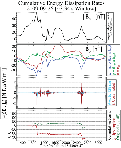
Figure 11: This example shows the same time range as Figure 10 and the top two panels are the same. The third panel shows $\left(-\textbf{j}{{}_{o}}\cdot\delta\textbf{E}\right)$ at the $\delta$E time steps (red) with corresponding trend line (cyan). The fourth panel shows the cumulative sum of $\left(-\textbf{j}{{}_{o}}\cdot\delta\textbf{E}\right)$ at the $\delta$E time steps (red) and at j_o time steps (green).

F.2 Asymmetric Fluctuations

In this appendix we present an illustrative example that shows there is a net change in $\left(-\textbf{j}{{}_{o}}\cdot\delta\textbf{E}\right)$ across the high frequency waves of interest. Were this not the case, then the waves would not be able to impart momentum/energy to the particles, thus they could not produce a net work on the unit volume.

Figure 11 shows the same time range as Figures 3 and 10. The top two panels are the magnitude of B_o and its NCB components. The third panel is the same as the last panel of Figure 3. The fourth panel shows the cumulative sum of $\left(-\textbf{j}{{}_{o}}\cdot\delta\textbf{E}\right)$ at two different time steps. The green line was calculated by downsampling $\delta$E to the original B_o time stamps before calculating $\left(-\textbf{j}{{}_{o}}\cdot\delta\textbf{E}\right)$ and then summing. The red line shows the result when j_o is upsampled to the $\delta$E time steps before calculating $\left(-\textbf{j}{{}_{o}}\cdot\delta\textbf{E}\right)$ (corresponding to red line in third panel).

The main point of this figure is to show that the high frequency waves that we focus on in this study can produce a net change in $\left(-\textbf{j}{{}_{o}}\cdot\delta\textbf{E}\right)$. This means that the waves have lost electromagnetic energy to the particles, thus dissipating energy. Figure 11 shows that our main results presented in Figure 4 are reliable. Meaning, the time-average of $\left(-\textbf{j}{{}_{o}}\cdot\delta\textbf{E}\right)$ across the waves is not zero so that we have not neglected the restoring effects by using $\left\lvert\textbf{j}{{}_{o}}\cdot\delta\textbf{E}\right\rvert$.

In addition, we examined the cumulative sum of $\delta$S to determine if the waves carried a net energy flux. The results (not shown) are similar to those found for $\left(-\textbf{j}{{}_{o}}\cdot\delta\textbf{E}\right)$, namely, that the waves showed a net change in $\delta$S. Were these modes pure sinusoidal circularly polarized electromagnetic oscillations, the cumulative sum of $\delta$S would be zero.

Appendix G Removal of Secondary Ions

Onboard particle distribution moments (or moments calculated from telemetered particle distributions) can suffer from inaccuracies due to spacecraft charging [e.g., Génot and Schwartz, 2004; Geach et al., 2005; Davis et al., 2008], multiple species [e.g., Paschmann and Daly, 1998], multiple components [e.g., Wüest, M., Evans, D. S., & von Steiger, R., 2007], and limited energy ranges (e.g., V_Ti $\gtrsim$ V_bulk). Below we discuss how we accounted for these potential inaccuracies when examining the velocity distribution function moments.

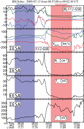
Figure 12: The figure shows an example bow shock crossing with the smoothed B_o and B_o (nT, first panel), V_bulk (km/s, second panel), N_i (cm^-3, third panel), T_e (eV, fourth panel), and T_i (eV, fifth panel). The region shaded in blue defines the downstream (i.e., magnetosheath) and red the upstream (i.e., solar wind). The data was measured by THEMIS-B.

Figure 12 shows an outbound bow shock crossing observed by THEMIS-B on 2009-07-13. The shock ramp center was $\sim$08:59:46 UT and THEMIS-B was at a GSE position of $\sim$$<$$+$11.5, $+$1.0, -2.2$>$ R_E. Shock waves, by definition, result in an increase in N_i, B_o, T_e, and T_i on the downstream(shocked) side of the transition region. The increase in temperature allows V_bulk to decrease to a subsonic value. In Figure 12 we observed an increase in N_i, B_o, and T_e with corresponding decrease in V_bulk, suggesting this was indeed a shock crossing. However, one can immediately see that the ions appear to be hotter (5th panel of Figure 12) on the upstream(unshocked) rather than the downstream(shocked) side. Therefore, the decrease in T_i across the transition region coupled with our knowledge of potential secondary ion contamination (e.g., shock-reflected ions) led us to examine the ion velocity moments in greater detail.

It is well known that the terrestrial bow shock is capable of producing multiple populations of reflected ions [e.g., Bonifazi and Moreno, 1981a, b; Fuselier et al., 1986]. Therefore, we initially assumed that these secondary ions were responsible for some fraction of the error in the ion velocity moments. To test whether ion beams were contaminating the upstream ion velocity moments, we examined the entire ion velocity distribution functions in three different reference frames and three different projections. To do this, we converted our observations to phase(velocity) space densities, translated the data into the new reference frame, rotated the data into physically significant coordinate basis (discussed below), and projected the triangulated results onto the three planes comprising this new coordinate basis.

Figure 13 shows contours of constant phase space density projected onto three planes (rows) and in three reference frames (first three columns). The first reference frame (first column) shown is the spacecraft frame. The second reference frame (second column) was defined by the level-2 average bulk flow velocity, V_bulk. The third reference frame (third column) shows the distribution plotted in the ion core bulk flow rest frame. The physically significant coordinate basis we used was defined by the value used for V_bulk and the observed quasi-static magnetic field, B_o (shaded planes in fourth column). These distributions do not assume gyrotropy.

This adjustment to V_bulk that resulted in the third column was determined by plotting the distributions in a manner similar to that shown in Figure 13 and then iteratively changing our estimate for V_bulk until the core of the distribution was centered on the origin in all three planes. We made this adjustment by starting in the second reference frame (second column) and adjusting V_bulk until the peak of the distribution rested at the origin (third column of Figure 13). Then we found the difference between this reference frame and the level-2 estimate for V_bulk to get our adjustment. It is important to note that when plotting particle velocity distributions in this manner that the reference frame and coordinate basis can strongly influence the results, as shown in Figure 13. For instance, in the spacecraft frame of reference (first column), the secondary population is not obviously a field-aligned beam. However, in the core bulk flow rest frame (third column), the signature of a strong field-aligned beam is obvious. We observed this beam for several minutes upstream of this shock ramp.

Figure 13: An example THEMIS IESA Burst particle velocity distribution observed upstream of a bow shock crossing. The three columns of contour plots correspond to three different rest frames defined by V_bulk at the top of each column. Each contour plot shows contours of constant phase space density (uniformly scaled from 1$\times$10^-14 to 1$\times$10^-8 s³cm^-3km^-3, where red is high) versus velocity projected onto three different planes defined by the shaded region in the coordinate axes shown in right-hand column. The velocity axes range from $\pm$2500 km/s and the crosshairs show the location of the origin.

Some previous studies have plotted foreshock ion velocity distributions in the spacecraft frame, however Figure 13 provides an example of why this can lead to confusion or a misinterpretation of the results. Note that the plane of projection in Figure 13 is dependent upon the definition of V_bulk. If the estimate for V_bulk or the plane of projection is inaccurate, then the projected distribution can be misleading. For instance, when comparing the results for the first plane (top row), one can see that the core of the second projection looks far more anisotropic than the core in the third projection. If one examines the bottom row of distributions, one can see surprisingly different results between the first and third columns. The apparent discrepancies are a consequence of the plotting routines, not a characteristic of the distribution. For more examples of these types of plots, see Wilson III et al. [2009, 2010, 2012].

After adjusting V_bulk, we created a mask to eliminate all secondary ion populations. We also removed ions within a small cone around the sun direction to reduce the effects of “UV contamination.” An example can be observed in the third distribution of the top row as the intense, narrow beam-like feature in the third quadrant near $\sim$500 km/s. We only applied these masks to those distributions with well defined secondary ion populations. After removing the secondary ions, we re-calculated the particle velocity moments. Therefore, these re-calculated velocity moments will reflect only the core of the ion distribution function.

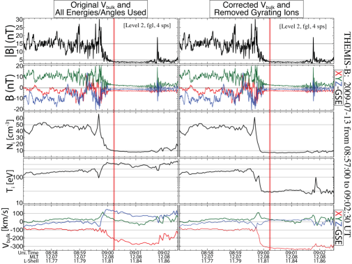
Figure 14: Comparison between the level-2 moments (left-hand column) and the estimates for the core only (right-hand column). The panels are as follows: B_o (nT, first panel), B_o (nT, second panel), N_i (cm^-3, third panel), T_i (eV, fourth panel), and V_bulk (km/s, fifth panel). The magnetic fields are identical in each column. The horizontal gray lines in each panel are to help the reader compare differences between the two results.

We show an example comparison between the original level-2 velocity moments and the core only estimates in Figure 14. The time range shown is the same as in Figure 12. The red shaded region corresponds to the time range of the ion velocity distribution shown in Figure 13. The results for T_i and V_bulk show dramatic differences, whereas N_i shows only minor differences in the upstream. The most important observations are that T_i now increases across the shock ramp and that $\mid$V_bulk$\mid$ shows differences of up to $\sim$30%. Not only did we observe large differences in $\mid$V_bulk$\mid$, one can see that there are significant changes in the flow direction as well.

There is a large amplitude magnetic fluctuations observed near $\sim$09:02 UT, which causes a deflection of the core V_bulk. We observed heating of the core ions and electrons near this structure as well. A comparison between the N_i plots in Figure 14 shows that the secondary ions were enhanced near this structure. When we examined the ion distributions (e.g., see Figure 13) we observed enhanced field-aligned and gyrophase-bunched ions near these fluctuations, consistent with recent observations [Wilson III et al., 2013b].

Upon examination of the results shown in Table 1, one can see that a few events have N_i2/N_i1 $>$ 4. There are many possible explanations for this, including but not limited to: (1) N_i1 does not include reflected particles; (2) the spacecraft velocity had a significant component along the shock plane; (3) time-variations due to single spacecraft observations; (4) inaccuracies in velocity moments due to V_Ti $\gtrsim$ V_bulk; (5) etc. Note that events with N_i2/N_i1 $>$ 4 are only in violation of a time-stationary neutral fluid approximations. If, for instance, the bow shock were being increasingly compressed as the spacecraft passed through the downstream region, one might expect N_i2/N_i1 $>$ 4.

References

- Angelopoulos et al. [2002] Angelopoulos, V., J. A. Chapman, F. S. Mozer, J. D. Scudder, C. T. Russell, K. Tsuruda, T. Mukai, T. J. Hughes, and K. Yumoto (2002), Plasma sheet electromagnetic power generation and its dissipation along auroral field lines, J. Geophys. Res., 107, 1181, doi:10.1029/2001JA900136.
- Auster et al. [2008] Auster, H. U., et al. (2008), The THEMIS Fluxgate Magnetometer, Space Sci. Rev., 141, 235–264, doi:10.1007/s11214-008-9365-9.
- Bale et al. [1998] Bale, S. D., P. J. Kellogg, D. E. Larson, R. P. Lin, K. Goetz, and R. P. Lepping (1998), Bipolar electrostatic structures in the shock transition region: Evidence of electron phase space holes, Geophys. Res. Lett., 25, 2929–2932, doi:10.1029/98GL02111.
- Bale et al. [2002] Bale, S. D., A. Hull, D. E. Larson, R. P. Lin, L. Muschietti, P. J. Kellogg, K. Goetz, and S. J. Monson (2002), Electrostatic Turbulence and Debye-Scale Structures Associated with Electron Thermalization at Collisionless Shocks, Astrophys. J., 575, L25–L28, doi:10.1086/342609.
- Bale et al. [2005] Bale, S. D., et al. (2005), Quasi-perpendicular Shock Structure and Processes, Space Sci. Rev., 118, 161–203, doi:10.1007/s11214-005-3827-0.
- Bale et al. [2008] Bale, S. D., et al. (2008), The Electric Antennas for the STEREO/WAVES Experiment, Space Sci. Rev., 136, 529–547, doi:10.1007/s11214-007-9251-x.
- Birn et al. [2008] Birn, J., J. E. Borovsky, and M. Hesse (2008), Properties of asymmetric magnetic reconnection, Phys. Plasmas, 15(3), 032,101, doi:10.1063/1.2888491.
- Bonifazi and Moreno [1981a] Bonifazi, C., and G. Moreno (1981a), Reflected and diffuse ions backstreaming from the earth’s bow shock. I Basic properties, J. Geophys. Res., 86, 4397–4413, doi:10.1029/JA086iA06p04397.
- Bonifazi and Moreno [1981b] Bonifazi, C., and G. Moreno (1981b), Reflected and diffuse ions backstreaming from the earth’s bow shock 2. Origin, J. Geophys. Res., 86, 4405–4414, doi:10.1029/JA086iA06p04405.
- Bonnell et al. [2008] Bonnell, J. W., F. S. Mozer, G. T. Delory, A. J. Hull, R. E. Ergun, C. M. Cully, V. Angelopoulos, and P. R. Harvey (2008), The Electric Field Instrument (EFI) for THEMIS, Space Sci. Rev., 141, 303–341, doi:10.1007/s11214-008-9469-2.
- Bougeret et al. [1995] Bougeret, J.-L., et al. (1995), Waves: The Radio and Plasma Wave Investigation on the Wind Spacecraft, Space Sci. Rev., 71, 231–263, doi:10.1007/BF00751331.
- Bougeret et al. [2008] Bougeret, J. L., et al. (2008), S/WAVES: The Radio and Plasma Wave Investigation on the STEREO Mission, Space Sci. Rev., 136, 487–528, doi:10.1007/s11214-007-9298-8.
- Breneman et al. [2011] Breneman, A. W., C. A. Cattell, L. B. Wilson III, K. Kersten, and K. Goetz (2011), STEREO observations of large amplitude electrostatic waves at the Earth’s bowshock, AGU Fall Meeting Abstracts, p. B2061.
- Cairns and McMillan [2005] Cairns, I. H., and B. F. McMillan (2005), Electron acceleration by lower hybrid waves in magnetic reconnection regions, Phys. Plasmas, 12, 102,110–+, doi:10.1063/1.2080567.
- Cattell et al. [2005] Cattell, C., et al. (2005), Cluster observations of electron holes in association with magnetotail reconnection and comparison to simulations, J. Geophys. Res., 110, 1211–+, doi:10.1029/2004JA010519.
- Comişel et al. [2011] Comişel, H., M. Scholer, J. Soucek, and S. Matsukiyo (2011), Non-stationarity of the quasi-perpendicular bow shock: comparison between Cluster observations and simulations, Ann. Geophys., 29, 263–274, doi:10.5194/angeo-29-263-2011.
- Coroniti [1970] Coroniti, F. V. (1970), Dissipation discontinuities in hydromagnetic shock waves, J. Plasma Phys., 4, 265–+, doi:10.1017/S0022377800004992.
- Cully et al. [2008] Cully, C. M., R. E. Ergun, K. Stevens, A. Nammari, and J. Westfall (2008), The THEMIS Digital Fields Board, Space Sci. Rev., 141, 343–355, doi:10.1007/s11214-008-9417-1.
- Davis et al. [2008] Davis, V. A., M. J. Mandell, and M. F. Thomsen (2008), Representation of the measured geosynchronous plasma environment in spacecraft charging calculations, J. Geophys. Res., 113, 10,204, doi:10.1029/2008JA013116.
- Dimmock et al. [2012] Dimmock, A. P., M. A. Balikhin, V. V. Krasnoselskikh, S. N. Walker, S. D. Bale, and Y. Hobara (2012), A statistical study of the cross-shock electric potential at low Mach number, quasi-perpendicular bow shock crossings using Cluster data, J. Geophys. Res., 117, A02210, doi:10.1029/2011JA017089.
- Dyrud and Oppenheim [2006] Dyrud, L. P., and M. M. Oppenheim (2006), Electron holes, ion waves, and anomalous resistivity in space plasmas, J. Geophys. Res., 111, 1302–+, doi:10.1029/2004JA010482.
- Edmiston and Kennel [1984] Edmiston, J. P., and C. F. Kennel (1984), A parametric survey of the first critical Mach number for a fast MHD shock., J. Plasma Phys., 32, 429–441.
- Ergun et al. [1998] Ergun, R. E., C. W. Carlson, J. P. McFadden, F. S. Mozer, L. Muschietti, I. Roth, and R. J. Strangeway (1998), Debye-Scale Plasma Structures Associated with Magnetic-Field-Aligned Electric Fields, Phys. Rev. Lett., 81, 826–829, doi:10.1103/PhysRevLett.81.826.
- Fishman et al. [1960] Fishman, F. J., A. R. Kantrowitz, and H. E. Petschek (1960), Magnetohydrodynamic Shock Wave in a Collision-Free Plasma, Rev. Modern Phys., 32, 959–966, doi:10.1103/RevModPhys.32.959.
- Forslund et al. [1972] Forslund, D., R. Morse, C. Nielson, and J. Fu (1972), Electron Cyclotron Drift Instability and Turbulence, Phys. Fluids, 15, 1303–1318, doi:10.1063/1.1694082.
- Forslund et al. [1970] Forslund, D. W., R. L. Morse, and C. W. Nielson (1970), Electron Cyclotron Drift Instability, Phys. Rev. Lett., 25, 1266–1270, doi:10.1103/PhysRevLett.25.1266.
- Franz et al. [2005] Franz, J. R., P. M. Kintner, J. S. Pickett, and L.-J. Chen (2005), Properties of small-amplitude electron phase-space holes observed by Polar, J. Geophys. Res., 110, 9212–+, doi:10.1029/2005JA011095.
- Fuselier et al. [1986] Fuselier, S. A., M. F. Thomsen, J. T. Gosling, S. J. Bame, and C. T. Russell (1986), Gyrating and intermediate ion distributions upstream from the earth’s bow shock, J. Geophys. Res., 91, 91–99, doi:10.1029/JA091iA01p00091.
- Gary [1981] Gary, S. P. (1981), Microinstabilities upstream of the earth’s bow shock - A brief review, J. Geophys. Res., 86, 4331–4336, doi:10.1029/JA086iA06p04331.
- Gary et al. [1994] Gary, S. P., E. E. Scime, J. L. Phillips, and W. C. Feldman (1994), The whistler heat flux instability: Threshold conditions in the solar wind, J. Geophys. Res., 99, 23,391–+, doi:10.1029/94JA02067.
- Geach et al. [2005] Geach, J., S. J. Schwartz, V. Génot, O. Moullard, A. Lahiff, and A. N. Fazakerley (2005), A corrector for spacecraft calculated electron moments, Ann. Geophys., 23, 931–943, doi:10.5194/angeo-23-931-2005.
- Génot and Schwartz [2004] Génot, V., and S. Schwartz (2004), Spacecraft potential effects on electron moments derived from a perfect plasma detector, Ann. Geophys., 22, 2073–2080, doi:10.5194/angeo-22-2073-2004.
- Gurgiolo et al. [1981] Gurgiolo, C., G. K. Parks, B. H. Mauk, K. A. Anderson, R. P. Lin, H. Reme, and C. S. Lin (1981), Non-E x B ordered ion beams upstream of the earth’s bow shock, J. Geophys. Res., 86, 4415–4424, doi:10.1029/JA086iA06p04415.
- Gurnett and Bhattacharjee [2005] Gurnett, D. A., and A. Bhattacharjee (2005), Introduction to Plasma Physics: With Space and Laboratory Applications, ISBN 0521364833. Cambridge, UK: Cambridge University Press.
- Hull et al. [2000] Hull, A. J., J. D. Scudder, R. J. Fitzenreiter, K. W. Ogilvie, J. A. Newbury, and C. T. Russell (2000), Electron temperature and de Hoffmann-Teller potential change across the Earth’s bow shock: New results from ISEE 1, J. Geophys. Res., 105, 20,957–20,972, doi:10.1029/2000JA900049.
- Hull et al. [2001] Hull, A. J., J. D. Scudder, D. E. Larson, and R. Lin (2001), Electron heating and phase space signatures at supercritical, fast mode shocks, J. Geophys. Res., 106, 15,711–15,734, doi:10.1029/2001JA900001.
- Hull et al. [2006] Hull, A. J., D. E. Larson, M. Wilber, J. D. Scudder, F. S. Mozer, C. T. Russell, and S. D. Bale (2006), Large-amplitude electrostatic waves associated with magnetic ramp substructure at Earth’s bow shock, Geophys. Res. Lett., 33, 15,104–+, doi:10.1029/2005GL025564.
- Hull et al. [2012] Hull, A. J., L. Muschietti, M. Oka, D. E. Larson, F. S. Mozer, C. C. Chaston, J. W. Bonnell, and G. B. Hospodarsky (2012), Multiscale whistler waves within Earth’s perpendicular bow shock, J. Geophys. Res., 117, A12104, doi:10.1029/2012JA017870.
- Jackson [1998] Jackson, J. D. (1998), Classical Electrodynamics, 3rd Edition, John Wiley & Sons, Inc., New York, NY.
- Kennel [1987] Kennel, C. F. (1987), Critical Mach numbers in classical magnetohydrodynamics, J. Geophys. Res., 92, 13,427–13,437, doi:10.1029/JA092iA12p13427.
- Kennel and Petscheck [1966] Kennel, C. F., and H. E. Petscheck (1966), Limit on stably trapped particle fluxes, J. Geophys. Res., 71, 1–28.
- Kennel et al. [1985] Kennel, C. F., J. P. Edmiston, and T. Hada (1985), A quarter century of collisionless shock research, in Collisionless Shocks in the Heliosphere: A Tutorial Review, Geophys. Monogr. Ser., vol. 34, edited by R. G. Stone and B. T. Tsurutani, pp. 1–36, AGU, Washington, D.C.
- Koval and Szabo [2008] Koval, A., and A. Szabo (2008), Modified “Rankine-Hugoniot” shock fitting technique: Simultaneous solution for shock normal and speed, J. Geophys. Res., 113, 10,110–+, doi:10.1029/2008JA013337.
- Krasnoselskikh et al. [2002] Krasnoselskikh, V. V., B. Lembège, P. Savoini, and V. V. Lobzin (2002), Nonstationarity of strong collisionless quasiperpendicular shocks: Theory and full particle numerical simulations, Phys. Plasmas, 9, 1192–1209, doi:10.1063/1.1457465.
- Lampe et al. [1972] Lampe, M., W. M. Manheimer, J. B. McBride, J. H. Orens, K. Papadopoulos, R. Shanny, and R. N. Sudan (1972), Theory and Simulation of the Beam Cyclotron Instability, Phys. Fluids, 15, 662–675, doi:10.1063/1.1693961.
- Le Contel et al. [2008] Le Contel, O., et al. (2008), First Results of the THEMIS Search Coil Magnetometers, Space Sci. Rev., 141, 509–534, doi:10.1007/s11214-008-9371-y.
- Lobzin et al. [2007] Lobzin, V. V., V. V. Krasnoselskikh, J. Bosqued, J. Pinçon, S. J. Schwartz, and M. Dunlop (2007), Nonstationarity and reformation of high-Mach-number quasiperpendicular shocks: Cluster observations, Geophys. Res. Lett., 34, 5107–+, doi:10.1029/2006GL029095.
- Lu et al. [2008] Lu, Q. M., B. Lembège, J. B. Tao, and S. Wang (2008), Perpendicular electric field in two-dimensional electron phase-holes: A parameter study, J. Geophys. Res., 113, 11,219–+, doi:10.1029/2008JA013693.
- Matsukiyo and Scholer [2006] Matsukiyo, S., and M. Scholer (2006), On microinstabilities in the foot of high Mach number perpendicular shocks, J. Geophys. Res., 111, 6104–+, doi:10.1029/2005JA011409.
- Mazelle et al. [2010] Mazelle, C., B. Lembège, A. Morgenthaler, K. Meziane, T. S. Horbury, V. Génot, E. A. Lucek, and I. Dandouras (2010), Self-Reformation of the Quasi-Perpendicular Shock: CLUSTER Observations, Twelfth International Solar Wind Conference, 1216, 471–474, doi:10.1063/1.3395905.
- McFadden et al. [2008a] McFadden, J. P., C. W. Carlson, D. Larson, M. Ludlam, R. Abiad, B. Elliott, P. Turin, M. Marckwordt, and V. Angelopoulos (2008a), The THEMIS ESA Plasma Instrument and In-flight Calibration, Space Sci. Rev., 141, 277–302, doi:10.1007/s11214-008-9440-2.
- McFadden et al. [2008b] McFadden, J. P., C. W. Carlson, D. Larson, J. Bonnell, F. Mozer, V. Angelopoulos, K.-H. Glassmeier, and U. Auster (2008b), THEMIS ESA First Science Results and Performance Issues, Space Sci. Rev., 141, 477–508, doi:10.1007/s11214-008-9433-1.
- Mellott and Greenstadt [1984] Mellott, M. M., and E. W. Greenstadt (1984), The structure of oblique subcritical bow shocks - ISEE 1 and 2 observations, J. Geophys. Res., 89, 2151–2161, doi:10.1029/JA089iA04p02151.
- Meziane et al. [1997] Meziane, K., et al. (1997), Wind observation of gyrating-like ion distributions and low frequency waves upstream from the earth’s bow shock, Adv. Space Res., 20, 703–706, doi:10.1016/S0273-1177(97)00459-6.
- Mitchell et al. [2012] Mitchell, J. J., S. J. Schwartz, and U. Auster (2012), Electron cross talk and asymmetric electron distributions near the Earth’s bowshock, Ann. Geophys., 30, 503–513, doi:10.5194/angeo-30-503-2012.
- Mozer and Sundkvist [2013] Mozer, F. S., and D. Sundkvist (2013), Electron Heating in Quasi-Perpendicular Shocks, ArXiv e-prints.
- Muschietti and Lembège [2013] Muschietti, L., and B. Lembège (2013), Microturbulence in the electron cyclotron frequency range at perpendicular supercritical shocks, J. Geophys. Res., doi:10.1002/jgra.50224, in press.
- Parks et al. [2012] Parks, G. K., et al. (2012), Entropy Generation across Earth’s Collisionless Bow Shock, Phys. Rev. Lett., 108, 061102, doi:10.1103/PhysRevLett.108.061102.
- Paschmann and Daly [1998] Paschmann, G., and P. W. Daly (1998), Analysis Methods for Multi-Spacecraft Data. ISSI Scientific Reports Series SR-001, ESA/ISSI, Vol. 1. ISBN 1608-280X, 1998, ISSI Sci. Rep. Ser., 1.
- Petkaki and Freeman [2008] Petkaki, P., and M. P. Freeman (2008), Nonlinear Dependence of Anomalous Ion-Acoustic Resistivity on Electron Drift Velocity, Astrophys. J., 686, 686–693, doi:10.1086/590654.
- Petkaki et al. [2006] Petkaki, P., M. P. Freeman, T. Kirk, C. E. J. Watt, and R. B. Horne (2006), Anomalous resistivity and the nonlinear evolution of the ion-acoustic instability, J. Geophys. Res., 111, 1205–+, doi:10.1029/2004JA010793.
- Petschek [1958] Petschek, H. E. (1958), Aerodynamic Dissipation, Rev. Mod. Phys., 30, 966–974, doi:10.1103/RevModPhys.30.966.
- Riquelme and Spitkovsky [2011] Riquelme, M. A., and A. Spitkovsky (2011), Electron Injection by Whistler Waves in Non-relativistic Shocks, Astrophys. J., 733, 63–+, doi:10.1088/0004-637X/733/1/63.
- Roux et al. [2008] Roux, A., O. Le Contel, C. Coillot, A. Bouabdellah, B. de La Porte, D. Alison, S. Ruocco, and M. C. Vassal (2008), The Search Coil Magnetometer for THEMIS, Space Sci. Rev., 141, 265–275, doi:10.1007/s11214-008-9455-8.
- Sagdeev [1966] Sagdeev, R. Z. (1966), Cooperative Phenomena and Shock Waves in Collisionless Plasmas, Rev. Plasma Phys., 4, 23–+.
- Schwartz et al. [2011] Schwartz, S. J., E. Henley, J. Mitchell, and V. Krasnoselskikh (2011), Electron Temperature Gradient Scale at Collisionless Shocks, Phys. Rev. Lett., 107, 215,002, doi:10.1103/PhysRevLett.107.215002.
- Scudder et al. [1986a] Scudder, J. D., T. L. Aggson, A. Mangeney, C. Lacombe, and C. C. Harvey (1986a), The resolved layer of a collisionless, high beta, supercritical, quasi-perpendicular shock wave. I - Rankine-Hugoniot geometry, currents, and stationarity, J. Geophys. Res., 91, 11,019–11,052, doi:10.1029/JA091iA10p11019.
- Scudder et al. [1986b] Scudder, J. D., T. L. Aggson, A. Mangeney, C. Lacombe, and C. C. Harvey (1986b), The resolved layer of a collisionless, high beta, supercritical, quasi-perpendicular shock wave. II - Dissipative fluid electrodynamics, J. Geophys. Res., 91, 11,053–11,073, doi:10.1029/JA091iA10p11053.
- Scudder et al. [1986c] Scudder, J. D., A. Mangeney, C. Lacombe, C. C. Harvey, and C. S. Wu (1986c), The resolved layer of a collisionless, high beta, supercritical, quasi-perpendicular shock wave. III - Vlasov electrodynamics, J. Geophys. Res., 91, 11,075–11,097, doi:10.1029/JA091iA10p11075.
- Shu [1992] Shu, F. H. (1992), Physics of Astrophysics, Vol. II, University Science Books, ISBN 0-935702-65-2.
- Spitzer and Härm [1953] Spitzer, L., and R. Härm (1953), Transport Phenomena in a Completely Ionized Gas, Phys. Rev., 89, 977–981, doi:10.1103/PhysRev.89.977.
- Sundkvist and Mozer [2013] Sundkvist, D., and F. Mozer (2013), Demagnetized Electron Heating at Collisionless Shocks, ArXiv e-prints.
- Sundkvist et al. [2012] Sundkvist, D., V. Krasnoselskikh, S. D. Bale, S. J. Schwartz, J. Soucek, and F. Mozer (2012), Dispersive Nature of High Mach Number Collisionless Plasma Shocks: Poynting Flux of Oblique Whistler Waves, Phys. Rev. Lett., 108, 025,002, doi:10.1103/PhysRevLett.108.025002.
- Tidman and Krall [1971] Tidman, D. A., and N. A. Krall (1971), Shock waves in collisionless plasmas, New York, NY: John Wiley & Sons, Inc.; ISBN:0-471-86785-3.
- Torrence and Compo [1998] Torrence, C., and G. P. Compo (1998), Wavelet Analysis Software, atmospheric and Oceanic Sciences, University of Colorado, Online: http://paos.colorado.edu/research/wavelets/.
- Treumann [2009] Treumann, R. A. (2009), Fundamentals of collisionless shocks for astrophysical application, 1. Non-relativistic shocks, Astron. & Astrophys. Rev., 17, 409–535, doi:10.1007/s00159-009-0024-2.
- Vedenov [1963] Vedenov, A. A. (1963), Quasi-linear plasma theory (theory of a weakly turbulent plasma), J. Nucl. Energy, 5, 169–186, doi:10.1088/0368-3281/5/3/305.
- Vinas and Scudder [1986] Vinas, A. F., and J. D. Scudder (1986), Fast and optimal solution to the ’Rankine-Hugoniot problem’, J. Geophys. Res., 91, 39–58, doi:10.1029/JA091iA01p00039.
- Wilson III [2010] Wilson III, L. B. (2010), The microphysics of collisionless shocks, Ph.D. thesis, University of Minnesota lynn.b.wilsoniii@gmail.com.
- Wilson III et al. [2007] Wilson III, L. B., C. Cattell, P. J. Kellogg, K. Goetz, K. Kersten, L. Hanson, R. MacGregor, and J. C. Kasper (2007), Waves in Interplanetary Shocks: A Wind/WAVES Study, Phys. Rev. Lett., 99(4), 041101, doi:10.1103/PhysRevLett.99.041101.
- Wilson III et al. [2009] Wilson III, L. B., C. A. Cattell, P. J. Kellogg, K. Goetz, K. Kersten, J. C. Kasper, A. Szabo, and K. Meziane (2009), Low-frequency whistler waves and shocklets observed at quasi-perpendicular interplanetary shocks, J. Geophys. Res., 114, A10106, doi:10.1029/2009JA014376.
- Wilson III et al. [2010] Wilson III, L. B., C. A. Cattell, P. J. Kellogg, K. Goetz, K. Kersten, J. C. Kasper, A. Szabo, and M. Wilber (2010), Large-amplitude electrostatic waves observed at a supercritical interplanetary shock, J. Geophys. Res., 115, A12104, doi:10.1029/2010JA015332.
- Wilson III et al. [2011] Wilson III, L. B., C. A. Cattell, P. J. Kellogg, J. R. Wygant, K. Goetz, A. Breneman, and K. Kersten (2011), The properties of large amplitude whistler mode waves in the magnetosphere: Propagation and relationship with geomagnetic activity, Geophys. Res. Lett., 38, L17107, doi:10.1029/2011GL048671.
- Wilson III et al. [2012] Wilson III, L. B., et al. (2012), Observations of electromagnetic whistler precursors at supercritical interplanetary shocks, Geophys. Res. Lett., 39, L08109, doi:10.1029/2012GL051581.
- Wilson III et al. [2013a] Wilson III, L. B., et al. (2013a), Electromagnetic waves and electron anisotropies downstream of supercritical interplanetary shocks, J. Geophys. Res., 118, 5–16, doi:10.1029/2012JA018167.
- Wilson III et al. [2013b] Wilson III, L. B., et al. (2013b), Shocklets, SLAMS, and field-aligned ion beams in the terrestrial foreshock, J. Geophys. Res., 118, 957–966, doi:10.1029/2012JA018186.
- Wu et al. [1983] Wu, C. S., D. Winske, K. Papadopoulos, Y. M. Zhou, S. T. Tsai, and S. C. Guo (1983), A kinetic cross-field streaming instability, Phys. Fluids, 26, 1259–1267, doi:10.1063/1.864285.
- Wu et al. [1984] Wu, C. S., et al. (1984), Microinstabilities associated with a high Mach number, perpendicular bow shock, Space Sci. Rev., 37, 63–109, doi:10.1007/BF00213958.
- Wüest, M., Evans, D. S., & von Steiger, R. [2007] Wüest, M., Evans, D. S., & von Steiger, R. (Ed.) (2007), Calibration of Particle Instruments in Space Physics, ESA Publications Division, Keplerlaan 1, 2200 AG Noordwijk, The Netherlands.
- Wygant et al. [2000] Wygant, J. R., et al. (2000), Polar spacecraft based comparisons of intense electric fields and Poynting flux near and within the plasma sheet-tail lobe boundary to UVI images: An energy source for the aurora, J. Geophys. Res., 105, 18,675–18,692, doi:10.1029/1999JA900500.
- Yoon and Lui [2006] Yoon, P. H., and A. T. Y. Lui (2006), Quasi-linear theory of anomalous resistivity, J. Geophys. Res., 111, 2203–+, doi:10.1029/2005JA011482.
- Yoon and Lui [2007] Yoon, P. H., and A. T. Y. Lui (2007), Anomalous resistivity by fluctuation in the lower-hybrid frequency range, J. Geophys. Res., 112, 6207–+, doi:10.1029/2006JA012209.