Non-linear fate of internal wave attractors

Abstract

We present a laboratory study on the instability of internal wave attractors in a trapezoidal fluid domain filled with uniformly stratified fluid. Energy is injected into the system via standing-wave-type motion of a vertical wall. Attractors are found to be destroyed by parametric subharmonic instability (PSI) via a triadic resonance which is shown to provide a very efficient energy pathway from long to short length scales. This study provides an explanation why attractors may be difficult or impossible to observe in natural systems subject to large amplitude forcing.

Introduction. Energy transfer from large to small-scale is a critical issue in the dynamics of large geophysical systems such as ocean and atmosphere. In this context, internal waves are of particular interest due to their specific dispersion and reflection properties. In a uniformly stratified fluid of infinite extent, which is the usual simplification of a realistic slow-varying stratification, internal waves propagate as oblique beams obeying Phillips1966 the following dispersion relation $\theta=\mbox{arccos}{(\omega/N)}$, where $\theta$ is the angle between the wave beams and the vertical, $\omega$ the wave frequency, $N=[-(g/\rho)(d\rho/dz)]^{1/2}$ the constant buoyancy frequency, and $\rho(z)$ the density stratification a function of the vertical coordinate $z$. Consequently, the beam angle with respect to the vertical is preserved when the beam is reflected at a rigid boundary. These restrictive conditions give a purely geometrical reason for strong variations of scale (focusing or defocusing) when an internal-wave beam is reflected at a sloping boundary. The complex dynamics of this phenomenon has been extensively studied Dauxois1999 ; Swinney2008 .

In confined fluid domains, focusing usually prevails: successive reflections of internal wave beams at rigid boundaries produce interestingly nearly closed loops which gradually converge toward a closed trajectory, an internal wave attractor Maas1995 . Ray trajectories in arbitrary shaped containers are generally not closed, and therefore energy injected in the domain is evenly distributed. On the contrary, when an attractor is present as in Fig. 1a, essentially all the energy is concentrated on a few beams defining the limit cycle and, consequently, injected energy being focused, nonlinear instabilites are more likely to be expected. Experimentally, an attractor was first demonstrated in a trapezoidal domain filled with uniformly stratified fluid Maas1997 . Simplistic considerations of wave-ray billiard lead to the unphysical conclusion of vanishingly small width of attractor branches (infinite focusing). In reality, a finite width of wave beams is set by the balance between geometric focusing and viscous broadening Hazewinkel2008 ; Grisouard2008 . Attractors were shown to be sufficiently robust to be observable in a non-uniform stratification and in test tanks with corrugated walls Hazewinkel2010 as well as in laterally infinite fluid domains with appropriate bottom topography Echeverry2011 . The significance of wave attractors has been recognized in rotating fluids Rieutord2000 and proposed for magnetized materials Maas2005 .

Theoretical studies on the behavior of a hyperbolic system describing attractor-like structures in confined domains reveal highly complicated dynamics. However, this rich dynamics arises in strictly linear PDEs, which form the background of existing theoretical studies Maas2005 . Numerically, nearly all studies of wave attractors solve linear equations of motion as stressed in Grisouard2008 . Experimentally, attractors are usually generated by low-amplitude vertical or horizontal oscillations of test tanks filled with stratified fluids Maas1997 ; Hazewinkel2008 ; Hazewinkel2010 or by a modulation of the angular velocity in rotating fluids Manders2003 . Oscillations of small objects have also been used to produce internal waves forming attractor-like patterns in 2D Maas2005 and 3D Hazewinkel2011 geometries. Experimentally observed attractors had therefore relatively low energy and their behavior can be explained by linear mechanisms. In this connection, a number of important questions arise. What happens to wave attractors as the amount of injected energy increases? What is the main mechanism of instability which destroys wave attractors? Does the instability produce new length scales which are shorter than the equilibrium width Hazewinkel2008 of attractor? What is beyond the instability? In the present letter, we address all these issues experimentally.

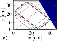
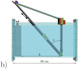
Figure 1: (Color online) Panel (a) presents the prediction of a wave-ray billiard with a bottom length $L=$45.6\text{\,}\mathrm{c}\mathrm{m}$$ and a depth $H=$32.6\text{\,}\mathrm{c}\mathrm{m}$$, while the sloping wall is inclined at an angle $\alpha=30^{\circ}$ with the vertical. The ray direction (defined by the group velocity) of the limit-cycle is counter-clockwise as shown by red arrows. Panel (b): Corresponding experimental setup showing the wave generator and the sloping wall inside the immobile tank of size $80\times 17\times 42.5$ cm. The working bottom length of the section, the depth and the sloping angle are the one given in panel (a). Conventional double-bucket technique is used to create a uniform stratification with a buoyancy frequency $N=$0.95\text{\,}\mathrm{r}\mathrm{a}\mathrm{d}\mathrm{/}\mathrm{s}$$.

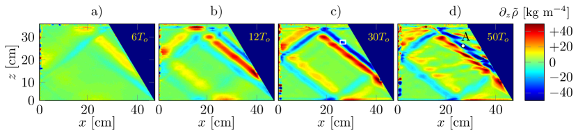
Figure 2: (Color online) Snapshots of the vertical density gradient field for $t=6T_{0}$ (a), $12T_{0}$ (b), $30T_{0}$ (c), $50T_{0}$ (d) where $T_{0}=2\pi/\omega_{0}$ is the primary wave period. Note that the shade (color online) scale is the same in all panels. The wave frequency is $\omega_{0}/N=0.62\pm 0.02$ and the motion amplitude of the plates of the generator is set to $a=0.25$ cm. The small white rectangle in panel (c) defines the acquisition region used for computing the time-frequency spectrum used for Fig. 4.

Experiment. To generate internal wave attractors with a high level of injected energy, we use a novel approach, presented in Fig. 1b. Experiments are performed in a quiescent test tank. The classic trapezoidal geometry Maas1997 is designed with a sliding sloping wall which can be slowly inserted into the fluid once the test tank is filled. The energy is injected into the experimental system by the internal wave generator Gostiaux2007 ; Mercier2010 ; Joubaud2012 tuned to produce the first vertical mode for internal waves in finite depth $H$. The time dependent profile of the generator, and therefore of the left side of the tank, is given by

$$\eta(z,t)=a\cos(\pi z/H)\cos(\omega_{0}t)\,,$$ (1)

where $a$ is its amplitude. The profile (1) is reproduced in discrete stepwise form by the motion of 51 horizontal plates driven by the rotation of a vertical camshaft. Since the thickness of each plate is small compared to the width of the wave-attractor beams, the discretization does not produce any secondary perturbations to the wave field, in agreement with Hazewinkel2010 ; Mercier2010 . The perturbations of the density gradient are evaluated with the synthetic schlieren technique Dalziel2000 from apparent displacements of elements of the background random dot pattern placed behind the test tank. A series of experiments has been performed varying the parameters $a\in[0.15,0.5]$ cm, $\omega_{0}/N\in[0.49,0.83]$ and $\alpha=15$ or 30^∘. We will emphasize now the cases $\alpha=30^{\circ}$ and $\omega/N=0.62$, but it is important to stress that all results are fully reproducible and lead to similar conclusions.

Results and discussion. The evolution of observed internal wave patterns with time is presented in Fig. 2 for a moderately large amplitude $a=0.25$ cm. One can see that the attractor reaches its fully developed state after a transient of roughly 30 periods of oscillation of the generator $T_{0}=2\pi/\omega_{0}$. The direction of this (1,1) attractor (one reflection at the surface and one reflection at the vertical sidewall) is counter-clockwise in agreement with dominant focusing effects in bucket geometry Maas1995 ; Maas1997 .

At a later stage, which is emphasized by Fig. 2d presenting the snapshot $t=50T_{0}$, an instability builds up in the most energetic (focusing) branch of the wave attractor. Figures 3 show precisely the time-serie recorded in the focusing branch of the wave attractor. It is clearly apparent that once the generator has been switched on, the amplitude of the horizontal density gradient field increases: then, as one could expect from the inspection of the first three snapshots of Figs. 2, an equilibrium value is reached after slightly more than 20 periods. However, it is also visible that, for amplitude $a$ larger than 0.25, the motion is much less regular in a later stage, corresponding presumably to a superposition of several components.

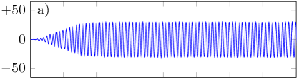
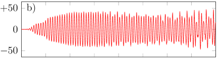
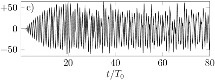
Figure 3: (Color online) Evolution versus time of the amplitude of $\partial_{x}\tilde{\rho}$ in the focusing branch of the internal wave attractor, measured in point A defined in Fig. 2d. The different panels correspond to different values of the injected energy measured through the amplitude of the cames: $a=$0.2 cm (a), 0.25 cm (b) and 0.5 cm (c).

Figure 2d reveals that the instability develops in form of oblique distortions of the wave beam, reminiscent of a typical pattern of parametric subharmonic instability (PSI) via triadic resonance Joubaud2012 ; Bourget2013 . The studies on wave-wave interactions, including triadic resonance, has a long history Phillips1981 . The significance of triadic resonance among other possible mechanisms of internal-wave instability in oceanographic applications is a debated issue Sutherland2006 . However, there is a growing body of evidence Joubaud2012 ; Bourget2013 ; KoudellaStaquet ; JenniferKraig ; Mattew that it is a major mechanism of instability in many practical circumstances. Energy transfer from the primary wave to two secondary waves is known to be possible when wave frequencies and wave vectors satisfy both the temporal

$$\omega_{0}=\omega_{1}+\omega_{2}$$ (2)

and the spatial

$${\bf k}_{0}={\bf k}_{1}+{\bf k}_{2}$$ (3)

conditions for triadic resonance, where subscripts 0, 1 and 2 refer to the primary, and both secondary waves, respectively. Let us check the fulfillment of Eqs. (2) and (3) in our case.

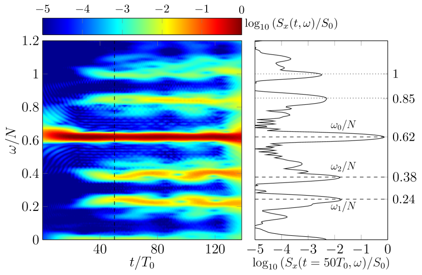
Figure 4: (Color online) (a) Time frequency spectrum $S_{x}(\omega,t)$ of the horizontal density gradient field for $a=0.25$ cm. Data were averaged on the small white rectangle shown in Fig. 2(c). (b) Frequency spectrum $S_{x}(\omega,t=50T_{0})$. The quantity $S_{0}$ is defined as the time average of the main component $\langle S_{x}(\omega_{0},t)\rangle$.

Figure 4 presents the time-frequency spectrum, defined as in Joubaud2012 ; Bourget2013 , of an area in the focusing branch of the attractor. This picture confirms that the amplitude of the main frequency component reached quickly its asymptotic value, however this representation emphasizes also that the frequency content is very rich. The main frequency components revealed via time-frequency analysis are listed in Table 1. The measured frequency of the primary wave is equal to the forcing frequency $\omega_{0}$, while the values for the secondary waves show that the temporal resonance condition (2) is satisfied with a good accuracy. All frequencies satisfy the dispersion relation individually. For the sake of completeness, note that two smaller peaks are also visible in Fig. 4 thanks to the logarithmic scale. Corresponding to the buoyancy frequency $N$ and $N\cos\alpha$, the oscillations along the inclined wall, these two natural frequencies are excited as expected for a nonlinear system.

Location	Subscript	$\omega/N$	$\ell$	$m$	$\left|{\bf k}\right|$
			[m-1]	[m-1]	[m-1]
Injection	*	0.62	+7.6	$\pm$ 9.6	12.3
Attractor	0	0.62	-64 ($\pm 1$)	-76 ($\pm 1$)	99
Attractor	1	0.24	+39 ($\pm$ 5)	+177 ($\pm 10$)	181
Attractor	2	0.38	-108 ($\pm 3$)	-265 ($\pm 3$)	287

Table 1: Main frequency values of the attractor determined with the time-frequency values and the corresponding values of the wave vector components $(\ell,m)$ that have been measured with the Hilbert transform Mercier2008 . Both components of the wave vector have been computed with ${\bf k}=-\nabla\phi$ where $\phi$ corresponds to the phase shown in Fig. 5. Errors in measurements of $\bf k_{1}$ are larger as phase lines are more horizontal and the measurement zone near the slope is smaller. Characteristics of the initial injection are calculated from the frequency value and the vertical wave number $m_{*}=\pi/H=9.64~{}\textrm{m}^{-1}$.

The Hilbert transform, first introduced for internal-wave analysis in Mercier2008 , is a powerful tool for the investigation of PSI, especially to analyze the spatial resonance condition Joubaud2012 ; Bourget2013 . The results of filtering the raw data at frequencies $\omega_{0}$, $\omega_{1}$ and $\omega_{2}$ are presented in Fig. 5. The corresponding numerical data on the components of the primary and secondary wave vectors can be readily obtained by differentiating the phase with respect to both spatial variables; results are presented in Table 1. It can be seen that the spatial resonance condition (3) is satisfied with a reasonable accuracy ($\ell_{0}\simeq\ell_{1}+\ell_{2}$ and $m_{0}\simeq m_{1}+m_{2}$). In a uniformly stratified infinite wave guide of depth $H$, the injection of energy (1) generates a horizontally propagating first mode wave which can be represented as a sum of two oblique waves with opposite vertical wave numbers, which parameters are given in the first line of Table 1. The data of wave vectors involved in the triadic resonance show that the combination of the wave attractor with PSI provides an extremely efficient transfer from large to small length scales, namely from 12 to 290 m^-1 in wave numbers: the length of the secondary waves is roughly 25 times (!) shorter than the scale at which the energy is injected into the system. Note that the global Reynolds number in the experiment is $\displaystyle Re={a\omega_{0}H}/{\nu}\simeq 500$, where $\nu$ is the kinematic viscosity. In natural systems characterized by much larger values of the Reynolds number, we can expect an even larger difference between the length scales of input perturbation and secondary waves, which attests the quite dramatic energy transfer at play here Bourget2013 .

Figure 5: (Color online) The top (respectively bottom) row presents the real part (resp. phase) of the Hilbert transform at $t=50T_{0}$. Each column corresponds to a filtering around the following three frequencies: $\omega_{0}$, $\omega_{1}$ and $\omega_{2}$ in the first, second and third columns respectively. The phase is displayed only where the wave amplitude |$\partial_{x}\tilde{\rho}$| is larger than 15$\%$ of the maximum.

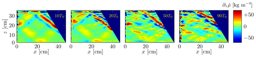
Figure 6: (Color online) Snapshots of the vertical density gradient field for $t=10T_{0}$ (a), $20T_{0}$ (b), $50T_{0}$ (c) and $90T_{0}$ (c) for a larger forcing amplitude $a=5$ mm. Note that the shade scale (color scale online) is the same in all panels.

This efficient energy transfer to short length scales occurs despite the rather small amplitude of the initial perturbation: indeed, the non-dimensional value $a/H=0.008$ leads already to a significant degradation of the wave attractor at large time of observation. It is therefore important to stress that these experimental results are in contrast with numerical results Grisouard2008 which successfully reproduced experiments of Hazewinkel2008 . However, in Ref. Grisouard2008 , at large input perturbation (an order of magnitude higher than the one used in the main run of simulations), authors have reported only weakly non-linear effects through wave components excited at multiples of the forcing frequency, i.e. at $2\omega$ and $3\omega$. No fingerprints of PSI were mentioned. A time frequency spectrum and a Hilbert transform analysis (not already popularized Mercier2008 ), would have been necessary to unambiguously clarify this. They were not provided.

As the amplitude of oscillation increases, the transfer of energy to short spatial scales intensifies. Figure 6 shows the evolution of the wave field at $a/H=0.015$ for a larger amplitude $a$=5 mm with the same experimental conditions and geometry depicted in Fig. 1. It can be seen that the instability sets in very quickly so that, finally, one can hardly distinguish an attractor in the wave field which consists of disintegrated patches and layers. For a different pattern of the attractor and high enough amplitude, PSI was also observed and the mechanism is unchanged as emphasized by Fig. 7.

Figure 7: (Color online) Left panel presents the prediction of a wave-ray billiard when $\omega_{0}/N=0.69\pm 0.01$ and $\alpha=30^{\circ}$. Right panel shows the snapshot of the vertical density gradient field for $t=30T_{0}$ and $a=0.25$ cm in which PSI is visible.

Interestingly, “patchiness” of internal wave beams has been reported in some oceanographic observations vanHaren2010 . The experimental results at the laboratory scale presented in this letter reproduce this effect, which hinders the observation of the attractor in real oceanographic conditions. In absence of the sloping wall, no PSI was reported for similar frequency and amplitude parameters Bourget2013 . Consequently, the present experimental arrangement is a “mixing box” since it allows very efficient destabilization of the internal wave field while using relatively low amplitudes of oscillation of the generator.

Conclusions. Previous theoretical, numerical and experimental literature on wave attractors is almost entirely focused on geometrical issues and linear mechanisms. In the present letter, we consider for the first time the ultimate instability of wave attractors. We use a new method of generation which allows an efficient injection of energy into internal-wave attractors. Attractors are created in a uniformly stratified fluid in a quiescent test tank with classic trapezoidal geometry by standing-wave-type motion of a vertical boundary.

We show that the energy injected into the system by the generator nicely focused on the wave attractor. As the amount of energy is increased (above $a=0.2$), the attractor is destroyed by parametric subharmonic instability (PSI) starting in the most energetic branch of the attractor and gradually eroding its structure. This two-step process provides an efficient energy transfer from the global scale associated to the size of the fluid domain to local scales associated with the secondary waves generated via triadic resonance. Beyond the instability, the attractor is transformed into a structure consisting of small-scale wave patches and layers, which hardly bear any resemblance to the classic attractor pattern coming from ray tracing or linear theoretical solution for the stream function. Therefore, even in nearly perfect geometrical conditions attractors may be very hard or impossible to observe in natural systems if the injected energy is too large to allow the existence of a stable attractor. Thus, the ability of attractors to concentrate wave energy places them at the origin of a spectacular energy cascade.

- (1) O.M. Phillips, Dynamics of the Upper Ocean, Cambridge University Press (1966).
- (2) T. Dauxois and W.R. Young, J. Fluid Mech. 390, 271 (1999).
- (3) H. P. Zhang, B. King, and H. L. Swinney, Phys. Rev. Lett. 100, 244504 (2008).
- (4) L.R.M. Maas and F.-P.A. Lam, J. Fluid Mech. 300, 1 (1995).
- (5) L.R.M. Maas, D. Benielli, J. Sommeria, and F.-P.A. Lam, Nature 388, 557 (1997).
- (6) N. Grisouard, C. Staquet, and I. Pairaud, J. Fluid Mech. 614, 1 (2008).
- (7) J. Hazewinkel, P. van Breevort, S.B. Dalziel, and L.R.M. Maas, J. Fluid Mech. 598, 373 (2008).
- (8) J. Hazewinkel, C. Tsimitri, L.R.M. Maas, and S.B. Dalziel, Phys. Fluids 22, 107 (2010).
- (9) P. Echeverri, T. Yokossi, N. J. Balmforth, and T. Peacock, J. Fluid Mech. 669, 354 (2011).
- (10) M. Rieutord, B. Georgeot, and L. Valdettaro, Phys. Rev. Lett. 85, 4277 (2000).
- (11) L.R.M. Maas, Int. J. Bifur. and Chaos 15, 2757 (2005).
- (12) A.M.M. Manders and L.R.M. Maas, J. Fluid Mech. 493, 59 (2003).
- (13) J. Hazewinkel, L.R.M. Maas, and S.B. Dalziel, Exps. Fluids 50, 247 (2011).
- (14) L. Gostiaux, H. Didelle, S. Mercier, and T. Dauxois, Exps. Fluids 42, 123 (2007).
- (15) M.J. Mercier, D. Martinand, M. Mathur, L. Gostiaux, T. Peacock, and T. Dauxois, J. Fluid Mech. 657, 308 (2010).
- (16) S. Joubaud, J. Munroe, P. Odier, and T. Dauxois, Phys. Fluids 24, 041703 (2012).
- (17) S.B. Dalziel, G.O. Hughes, and B.R. Sutherland, Exps. Fluids 28, 322 (2000).
- (18) B. Bourget, T. Dauxois, S. Joubaud, and P. Odier, J. Fluid Mech. in press (2013).
- (19) O.M. Phillips, J. Fluid Mech. 106, 215 (1981).
- (20) B.R. Sutherland, Phys. Fluids 18, 074107 (2006).
- (21) C. R. Koudella and C. Staquet, J. Fluid Mech. 548, 165 (2006).
- (22) J. A. MacKinnon and K. B. Winters, Geophys. Res. Lett. 32, L15605 (2005).
- (23) M. H. Alford, J. A. MacKinnon, Z. Zhao, R. Pinkel, J. Klymak and T. Peacock Geophys. Res. Lett. 34, L24601 (2007).
- (24) M.J. Mercier, N.B. Garnier, and T. Dauxois, Phys. Fluids 20, 086601 (2008).
- (25) H. van Haren, L.R.M. Maas, and T. Gerkema, Journal of Marine Research 68, 237 (2010).