Hierarchical dynamics for system-bath coherence correlation spectrum

Abstract

We propose a quasi-particle description for the hierarchical equations of motion formalism for quantum dissipative dynamics systems. Not only it provides an alternative mathematical means to the existing formalism, the new protocol clarifies also explicitly the physical meanings of the auxiliary density operators and their relations to full statistics on solvation bath variables. Combining with the standard linear response theory, we construct further the hierarchical dynamics formalism for correlated spectrum of system–bath coherence. We evaluate the spectrum matrix for a demonstrative spin-boson system-bath model. While the individual diagonal element of the spectrum matrix describes the system or the solvation bath correlation, the off-diagonal elements characterize the correlation between system and bath solvation dynamics.

The hierarchical equations of motion (HEOM) formalism has been established via the Feynman-Vernon path integral approach Tan906676 ; Xu05041103 ; Tan06082001 ; Xu07031107 ; Din12224103 and also the stochastic Liouville-equation approach.Yan04216 The numerical tractability of this exact quantum dissipation theory has been extensively demonstrated.Kre112166 ; Che11194508 ; Xu13024106 It is recognized that the auxiliary density operators (ADOs) in HEOM contain rich information on correlated system-bath coherence.Shi09164518 ; Zhu115678 Recently, Shi and coworkersZhu12194106 established an explicit relation between ADOs and moments of solvation coordinate. It is also noticed that ADOs in the conventional HEOM formalism are bosonic in nature, while those in the second-quantization (electronic) HEOM are fermionic.Jin08234703 ; Zhe121129 This observation implies the possibility of a quasi-particle picture that could offer further physical insights on ADOs.

In this work, we propose the dissipaton dynamics as a quasi-particle approach to the existing HEOM formalism for bosonic dissipative systems. Not only it clarifies the physical meanings of ADOs, the new approach leads also to an explicit HEOM evaluation for correlated system–bath coherence, including correlation functions for solvation bath variables. Throughout the paper we set $\hbar=1$ and $\beta=1/(k_{B}T)$. Denote also ${\cal L}(\cdot)\equiv[H_{\mbox{\tiny S}},(\cdot)]$, for the reduced system Liouvillian.

Let us start with the total composite Hamiltonian, $H_{\mbox{\tiny T}}=H_{\mbox{\tiny S}}+h_{\mbox{\tiny B}}+H_{\mbox{\tiny SB}}$, with the system-bath coupling the form of $H_{\mbox{\tiny SB}}=\sum_{a}Q_{a}F_{a}$. The system operator $Q_{a}$ here is called a dissipative mode and can be arbitrary, while the bath operator $F_{a}$ is called a solvation coordinate, for its being often modeled as a collection of harmonic bath coordinates. In the bare bath ($h_{\mbox{\tiny B}}$) interaction picture, $F^{\mbox{\tiny B}}_{a}(t)\equiv e^{ih_{\mbox{\tiny B}}t}F_{a}e^{-ih_{\mbox{\tiny B}}t}$. It is a stochastic variable, characterized by $\langle F^{\mbox{\tiny B}}_{a}\rangle_{\mbox{\tiny B}}=0$ and

$$C^{\mbox{\tiny B}}_{aa^{\prime}}(t)\equiv\langle F^{\mbox{\tiny B}}_{a}(t)F^{\mbox{\tiny B}}_{a^{\prime}}(0)\rangle_{\mbox{\tiny B}}=\frac{1}{\pi}\int_{-\infty}^{\infty}\!d\omega\frac{e^{-i\omega t}J_{aa^{\prime}}(\omega)}{1-e^{-\beta\omega}}.$$ (1)

The second identity is the bosonic fluctuation-dissipation theorem, with $J_{aa^{\prime}}(\omega)$ being the interacting bath spectral density.Yan05187 ; Wei08 The script “B” in Eq. (1) specifies the bath ensemble average, $\langle(\cdot)\rangle_{\mbox{\tiny B}}\equiv{\rm tr}_{\mbox{\tiny B}}[(\cdot)e^{-\beta h_{\mbox{\tiny B}}}]/{\rm tr}_{\mbox{\tiny B}}(e^{-\beta h_{\mbox{\tiny B}}})$, for the dynamical variables in the $h_{\mbox{\tiny B}}$-interaction picture. The full-space counterpart, $C_{aa^{\prime}}(t)$ [cf. Eq. (21)], is one of quantities subject to a direct HEOM evaluation later.

(A) The Dissipaton Approach to HEOM – In line with the HEOM construction,Tan906676 ; Xu05041103 ; Tan06082001 we decompose $C^{\mbox{\tiny B}}_{aa^{\prime}}(t)$ of Eq. (1), via certain sum-over-poles scheme, as

$$C^{\mbox{\tiny B}}_{aa^{\prime}}(t)\approx\sum_{k=1}^{K}\eta^{aa^{\prime}}_{k}e^{-\gamma^{aa^{\prime}}_{k}t}.$$ (2)

It would be exact if $K\rightarrow\infty$. For clarity we limit our discussion to the real-exponents ($\gamma^{aa^{\prime}}_{k}>0$) case such as in an overdamped phonon bath. The expansion coefficients ($\eta^{aa^{\prime}}_{k}$) are complex in general. Thus, each decomposition term in Eq. (2) represents a diffusive mode, which would be classified below as a dissipaton, involved in the HEOM dynamics of correlated system-bath coherence.

Introduce the so-called dissipaton operator, $\hat{f}^{ab}_{k}(t)$, having the color-$\gamma^{ab}_{k}$ and the statistical independence relation defined for $t>0$ as

$$\langle\hat{f}^{ab}_{k}(t)\hat{f}^{b^{\prime}a^{\prime}}_{k^{\prime}}(0)\rangle_{\mbox{\tiny B}}\equiv(\delta_{aa^{\prime}}\delta_{bb^{\prime}}\delta_{kk^{\prime}})\eta^{ab}_{k}\exp(-\gamma^{ab}_{k}t).$$ (3)

While $\langle\hat{f}^{ab}_{k}(0^{+})\hat{f}^{ba}_{k}\rangle_{\mbox{\tiny B}}=\eta^{ab}_{k}$, the discontinuity at $t=0$ is specified further with $\langle\hat{f}^{ab}_{k}(0^{-})\hat{f}^{ba}_{k}\rangle_{\mbox{\tiny B}}=(\eta^{ab}_{k})^{\ast}$ and $\langle\hat{f}^{ab}_{k}\hat{f}^{ba}_{k}\rangle_{\mbox{\tiny B}}={\rm Re}\,\eta^{ab}_{k}$. It is easy to show that individual solvation coordinates, preserving Eq. (2), can now be decomposed as

$$F_{a}=\sum_{b}\sum_{k=1}^{K}\hat{f}^{ab}_{k}.$$ (4)

As dissipatons are statistically independent, we can consider them individually, so that the indices are omitted, i.e., $\hat{f}^{ab}_{k}=\hat{f}$ and also for $\eta$ and $\gamma$, in the following dissipaton approach to HEOM. We will also exploit the property of a real-$\gamma$-colored dissipaton, as defined in Eq. (3). It is diffusive in the pure bath environment, satisfyingCha431

$$\text{tr}_{\mbox{\tiny B}}\big{[}\big{(}\tfrac{\partial}{\partial t}{\hat{f}}\big{)}_{\mbox{\tiny B}}\rho_{\mbox{\tiny T}}(t)\big{]}=-\gamma\,\text{tr}_{\mbox{\tiny B}}\!\big{[}{\hat{f}}\rho_{\mbox{\tiny T}}(t)\big{]}.$$ (5)

Here, $\big{(}\tfrac{\partial}{\partial t}{\hat{f}}\big{)}_{\mbox{\tiny B}}=-i[\hat{f},h_{\mbox{\tiny B}}]$ and $\rho_{\mbox{\tiny T}}(t)$ is the total system and bath composite density operator. Its bath trace, $\rho(t)\equiv{\rm tr}_{\mbox{\tiny B}}\rho_{\mbox{\tiny T}}(t)\equiv\rho_{0}(t)$, is the reduced system density operator and assigned to be the zeroth-tier ADO.

We will show below that $\rho_{n}(t)$, the $n^{\rm th}$-tier ADO in HEOM, is related to the $n$-number of irreducible dissipatons, denoted as $\big{(}\hat{f}^{n}\big{)}^{\circ}$, via

$$\rho_{n}(t)\equiv{\rm tr}_{\mbox{\tiny B}}\left[\big{(}\hat{f}^{n}\big{)}^{\circ}\rho_{\mbox{\tiny T}}(t)\right].$$ (6)

Introduce also

$$\rho_{n+\underline{m}}(t)\equiv{\rm tr}_{\mbox{\tiny B}}\left[\hat{f}^{m}\big{(}\hat{f}^{n}\big{)}^{\circ}\rho_{\mbox{\tiny T}}(t)\right],$$ (7)

with the underlined $\underline{m}$ specifying the $m$ dissipatons, $\hat{f}^{m}$, remained reducible. The Wick’s contraction theorem for Gaussian bath leads Eq. (7) to

$$\rho_{n+\underline{m}}=\rho_{n+1+\underline{m-1}}+n\eta\,\rho_{n-1+\underline{m-1}}\,.$$ (8)

For the system-bath coupling in the form of $H_{\mbox{\tiny SB}}=Q\hat{f}$, Eqs. (5)–(8), with $\underline{m}=\underline{1}$ and the Liouville-von Neumann equation, $\dot{\rho}_{\mbox{\tiny T}}(t)=-i[H_{\mbox{\tiny S}}+h_{\mbox{\tiny B}}+H_{\mbox{\tiny SB}},\rho_{\mbox{\tiny T}}(t)]$, lead immediately to

$$\dot{\rho}_{n} =-(i{\cal L}+n\gamma)\rho_{n}-i[Q,\rho_{n+1}]$$

$$\quad-in(\eta Q\rho_{n-1}-\eta^{\ast}\rho_{n-1}Q)\,.$$ (9)

This is just the well-established HEOM, constructed previously via the Feynman-Vernon path integral formulations.Tan906676 ; Tan06082001 ; Xu05041103 The physical meaning of ADOs are also self-evident via the remarkable relation, Eq. (6), to irreducible dissipatons.

(B) White Noise Residue Ansatz – It is well known that a modified HEOM formalism exploits a white noise residue (WNR) ansatz.Tan06082001 ; Xu07031107 ; Din12224103 To obtain the dissipaton prescription of this ansatz and other related issues hereafter, it would be sufficient to consider only the case of $C^{\mbox{\tiny B}}_{aa^{\prime}}(t)=0$ when $a\neq a^{\prime}$. The WNR ansatz starts with the interacting bath correlation function residue,

$$\delta C^{\mbox{\tiny B}}_{aa}(t)\equiv C^{\mbox{\tiny B}}_{aa}(t)-\sum_{k=1}^{K}\eta^{a}_{k}e^{-\gamma^{a}_{k}t}\simeq 2\Delta_{a}\delta(t).$$ (10)

Note that $\Delta_{a}$ is real. The associated solvation coordinate in dissipatons decomposition reads now

$$F_{a}=\sum_{k=1}^{K}\hat{f}^{a}_{k}+\delta\hat{F}_{a},$$ (11)

with the WNR dissipaton $\delta\hat{F}_{a}$ being of

$$\langle\delta\hat{F}^{\mbox{\tiny B}}_{a}(t)\delta\hat{F}^{\mbox{\tiny B}}_{a}(0)\rangle_{\mbox{\tiny B}}=2\Delta_{a}\delta(t)=\Delta_{a}\lim_{\Gamma\rightarrow\infty}\Gamma e^{-\Gamma t}.$$ (12)

An important implication here is the Lemma that there is at most one irreducible white-noise-dissipaton that can physically participate in. This Lemma will be verified via self-consistency with its consequences, as seen below.

Let us introduce the WNR to the case studied in Eq. (Hierarchical dynamics for system-bath coherence correlation spectrum), via setting now $H_{\mbox{\tiny SB}}=Q(\hat{f}+\delta\hat{F})$. It leads to Eq. (Hierarchical dynamics for system-bath coherence correlation spectrum) an additional term,

$$\dot{\rho}_{n}=\big{\{}\text{terms in Eq.\,(\ref{heom0})}\big{\}}-i[Q,\varrho_{n}],$$ (13)

with

$$\varrho_{n}(t)\equiv{\rm tr}_{\mbox{\tiny B}}\left[(\delta\hat{F})\big{(}\hat{f}^{n}\big{)}^{\circ}\rho_{\mbox{\tiny T}}(t)\right],$$ (14)

the one white-noise dissipaton counterpart of Eq. (6), satisfying $\dot{\varrho}_{n}=\big{\{}\text{Eq.\,(\ref{heom0}) with $\varrho$'s}\big{\}}-\Gamma\varrho_{n}-i\Gamma\Delta[Q,\rho_{n}]$. The last two terms arise from $\big{[}\tfrac{\partial}{\partial t}(\delta\hat{F})\big{]}_{\mbox{\tiny B}}$ and the contraction of two reducible white-noise dissipatons, respectively. The contribution from two irreducible white-noise dissipatons is zero, as inferred from the Lemma above. The convergence of $\dot{\varrho}_{n}$ in the limit of $\Gamma\rightarrow\infty$ leads therefore to the relation,

$$\varrho_{n}(t)=-i\Delta\big{[}Q,\rho_{n}(t)\big{]}.$$ (15)

This is an important result for a white-noise dissipaton. Substituting Eq. (15) into Eq. (13), we obtain

$$\dot{\rho}_{n} =-(i{\cal L}+n\gamma+\delta{\cal R})\rho_{n}-i[Q,\rho_{n+1}]$$

$$\quad-in(\eta Q\rho_{n-1}-\eta^{\ast}\rho_{n-1}Q)\,,$$ (16)

where $\delta{\cal R}(\cdot)=\Delta[Q,[Q,\,(\cdot)]]$. We have therefore recovered the modified HEOM formalism, constructed previously via the Feynman-Vernon path integral formulations. Tan06082001 ; Xu07031107 ; Din12224103 The proposed Lemma for white noise dissipaton is thus also verified.

The ADOs in the HEOM formalism are now completely identified as Eq. (6), or

$$\rho_{\sf n}(t)\equiv\rho_{n_{1}\cdots n_{K}}(t)={\rm tr}_{\mbox{\tiny B}}\!\left[\big{(}\hat{f}^{n_{K}}_{K}\big{)}^{\circ}\!\cdots\big{(}\hat{f}^{n_{1}}_{1}\big{)}^{\circ}\rho_{\mbox{\tiny T}}(t)\right].$$ (17)

For the multiple-dissipative modes case, each $\hat{f}^{n_{k}}_{k}$ above is understood further as a collection of $(\hat{f}^{ab}_{k})^{n^{ab}_{k}}$. The inclusion of white noise dissipatons does not add to the ADO indices, but via the relation of Eq. (15). Moreover, the multiple reducible white noise dissipatons counterparts of Eqs. (6) and (8) read

$$\varrho_{{\sf n};\underline{m}}(t) \equiv{\rm tr}_{\mbox{\tiny B}}\left[(\delta\hat{F})^{m}\big{(}\hat{f}^{n_{K}}_{K}\big{)}^{\circ}\cdots\big{(}\hat{f}^{n_{1}}_{1}\big{)}^{\circ}\rho_{\mbox{\tiny T}}(t)\right]$$

$$=\begin{cases}\quad\ (\delta\eta)^{j}\,\rho_{\sf n}(t),&m=2j\\ -i(\delta\eta)^{j}\,\Delta[Q,\rho_{\sf n}(t)],&m=2j+1\end{cases}\,.$$ (18)

Here, $\delta\eta\equiv\delta C^{\mbox{\tiny B}}_{aa^{\prime}}(t=0)$, via the first identity of Eq. (10). Apparently, $\varrho_{n;\underline{1}}(t)\equiv\varrho_{n}(t)$ of Eq. (14).

(C) Statistical Dynamics of Solvation Coordinates – Apparently, the zeroth-tier ADO amounts to the reduced system density operator, $\rho_{\sf n=\sf 0}(t)\equiv\rho(t)={\rm tr}_{\mbox{\tiny B}}\rho_{\mbox{\tiny T}}(t)$. The present identification of ADOs as Eq. (17) leads to HEOM further for the real-time dynamics of statistical solvation bath variables. For example, the moments of solvation coordinates, in relation to ADOs, can be readily identified, via Eqs. (11) and (17), together with the Wick’s contraction theorem of Eq. (8) and its white-noise limit of Eq. (Hierarchical dynamics for system-bath coherence correlation spectrum).

(D) Correlation Function for Solvation Coordinates – Another key result of this work is the establishment of the HEOM approach to correlation functions for solvation bath variables. Consider for illustration a two-mode case of $H_{\mbox{\tiny SB}}=Q_{a}F_{a}+Q_{b}F_{b}$, in which $\langle F^{\mbox{\tiny B}}_{a}(t)F^{\mbox{\tiny B}}_{b}(0)\rangle_{\mbox{\tiny B}}=0$, while $\langle F^{\mbox{\tiny B}}_{a^{\prime}}(t)F^{\mbox{\tiny B}}_{a^{\prime}}(0)\rangle_{\mbox{\tiny B}}=\eta_{a^{\prime}}e^{-\gamma_{a^{\prime}}t}+2\Delta_{a^{\prime}}\delta(t)$. Therefore,

$$F_{a^{\prime}}=\hat{f}_{a^{\prime}}+\delta\hat{F}_{a^{\prime}};\ \ \ \text{with $a^{\prime}=a$ or $b$}.$$ (19)

The corresponding ADOs are therefore

$$\rho_{n_{a},n_{b}}(t)={\rm tr}_{\mbox{\tiny B}}\!\left[\big{(}\hat{f}^{n_{b}}_{b}\big{)}^{\circ}\big{(}\hat{f}^{n_{a}}_{a}\big{)}^{\circ}\rho_{\mbox{\tiny T}}(t)\right].$$ (20)

Turn now to the cross-correlation function for solvation coordinates,

$$C_{ab}(t)=\langle F_{a}(t)F_{b}(0)\rangle={\rm Tr}\left\{F_{a}[{\cal G}_{\mbox{\tiny T}}(t)(F_{b}\rho^{\rm eq}_{\mbox{\tiny T}})]\right\},$$ (21)

with ${\cal G}_{\mbox{\tiny T}}(t)=e^{-i{\cal L}_{\mbox{\tiny T}}t}$ and $\rho^{\rm eq}_{\mbox{\tiny T}}=e^{-\beta H_{\mbox{\tiny T}}}/\text{Tr}e^{-\beta H_{\mbox{\tiny T}}}$, specified in the total system-and-bath composite space. Let

$$\rho_{\mbox{\tiny T}}(0;F_{b})\equiv F_{b}\rho^{\rm eq}_{\mbox{\tiny T}},$$ (22)

and $\rho_{\mbox{\tiny T}}(t;F_{b})={\cal G}_{\mbox{\tiny T}}(t)\rho_{\mbox{\tiny T}}(0;F_{b})$. Together with Eq. (19) for $a^{\prime}=a$, we can recast Eq. (21) in terms of ADOs as

$$C_{ab}(t)={\rm tr}_{\mbox{\tiny S}}\big{\{}\rho_{1,0}(t,F_{b})-i\Delta_{a}[Q_{a},\rho_{0,0}(t;F_{b})]\big{\}}.$$ (23)

The initial ADOs for the HEOM evaluation are determined with Eq. (22) for Eq. (20). After some simple algebra as described earlier, we obtain

$$\rho_{n_{a},n_{b}}(0;F_{b}) =\rho^{\rm eq}_{n_{a},n_{b}+1}+n_{b}\eta_{b}\rho^{\rm eq}_{n_{a},n_{b}-1}$$

$$\quad-i\Delta_{b}[Q_{b},\rho^{\rm eq}_{n_{a},n_{b}}].$$ (24)

The involving thermal equilibrium ADOs are obtained via the steady-state solutions. We have thus established the HEOM approach to correlation functions for solvation coordinates. As the HEOM evaluation on the system correlation functions has been well-established,Zhu115678 the present development extends its evaluation for both system and solvation bath dynamical variables.

(E) Numerical demonstrations – For demonstration, we consider a spin-boson system, $H_{\mbox{\tiny S}}=\frac{1}{2}\epsilon\sigma_{z}+V\sigma_{x}$, with the dissipative mode, $Q=\frac{1}{2}\sigma_{z}$, in terms of the Pauli matrixes. We set $\epsilon=50$ cm^-1 and $V=150$ cm^-1; thus the Rabi frequency of the bare system is $\Omega_{\rm R}=\sqrt{\epsilon^{2}+4V^{2}}=304$ cm^-1. The bath spectral density assumes $J(\omega)=2\lambda\gamma\omega/(\omega^{2}+\gamma^{2})$, with $\lambda=150$ cm^-1, but $\gamma=20$, 100, and 200 cm^-1, at $T=77$ and 298 K, separatively. We adopt the optimized HEOM formalismDin11164107 and the on-the-fly filtering propagator method that goes with the scaled ADOs.Shi09084105

We evaluate $\langle F(t)F(0)\rangle$ for the solvation coordinate, $\langle\sigma_{x}(t)\sigma_{x}(0)\rangle$ for the spin-system operator, and the cross-correlations between them, $\langle\sigma_{x}(t)F(0)\rangle$ and $\langle F(t)\sigma_{x}(0)\rangle$. Performing the half-Fourier transform on each of them,

$${\cal C}_{AB}(\omega)\equiv\int_{0}^{\infty}\!dt\,e^{i\omega t}\left[\langle A(t)B(0)\rangle-\langle A\rangle\langle B\rangle\right],$$ (25)

the spectrum via full-Fourier transform is then

$$S_{AB}(\omega)={\cal C}_{AB}(\omega)+{\cal C}^{\ast}_{BA}(\omega)=S^{\ast}_{BA}(\omega).$$ (26)

The detailed-balance relation, $S_{BA}(-\omega)=e^{-\beta\omega}S_{AB}(\omega)$, or its equivalent fluctuation-dissipation theorem,Yan05187 ; Wei08

$$\chi_{AB}(\omega)\equiv S_{AB}(\omega)-S_{BA}(-\omega)=(1-e^{-\beta\omega})S_{AB}(\omega),$$ (27)

is numerically verified in the following converged calculations. Apparently, $\chi_{AB}(\omega)=\chi^{\ast}_{BA}(\omega)=-\chi_{BA}(-\omega)$. While $\chi_{AA}(\omega)$ must be real, the off-diagonal $\{\chi_{AB}(\omega)\}$ of interest here are found to be also real, at least numerically. Consequently, $\chi_{AB}(\omega)=\chi_{BA}(\omega)=-\chi_{AB}(-\omega)$, for not just the diagonal but also the off-diagonal elements in study. The converged HEOM evaluation on the aforementioned correlation functions can therefore be conveniently reported in terms of the even function $\chi_{AB}(\omega)/\omega$, with $\chi_{AB}(\omega)/\omega\big{|}_{\omega=0}=\beta S_{AB}(0)$ [cf. Eq. (27)].

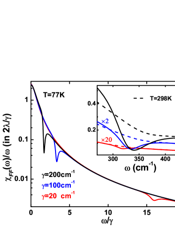
Figure 1: The evaluated $\chi_{FF}(\omega)/\omega$ at 77 K, for three values of the bath cutoff frequency, $\gamma=200\,{\rm cm}^{-1}$ (black), 100 cm^-1 (blue), and 20 cm^-1 (red). The inset shows the same function at both 77 K (solid) and 298 K (dash).

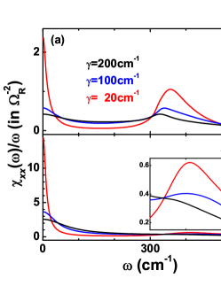
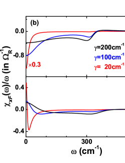
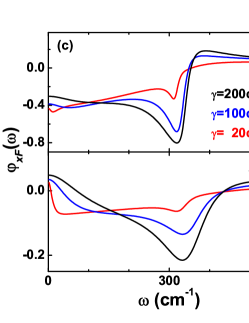
Figure 2: (a) The evaluated $\chi_{xx}(\omega)/\omega$ for system operator $\sigma_{x}$, (b) the $\chi_{xF}(\omega)/\omega$ for the cross-correlation of system $\sigma_{x}$ and bath $F$, and (c) the coherence spectrum $\varphi_{xF}(\omega)$ between system and bath, at 77 K (top) and 298 K (bottom), respectively.

Figure 1 reports the evaluated $\chi_{FF}(\omega)/\omega$ as function of $\omega/\gamma$, at 77 K. The bare-bath counterpart of this quantity is $J(\omega)/\omega=[1+(\omega/\gamma)^{2}]^{-1}(2\lambda/\gamma)$. The observed $\chi_{FF}(\omega)/\omega\big{|}_{\omega\rightarrow 0}>2\lambda/\gamma$ and the dips in Fig. 1 indicate the dominant energy flow from the system to bath in the low frequency regime, but vice verse in the effective system resonance regime, see also the inset of Fig. 1. These features are clearly enhanced as either $\gamma$ or $\beta$ increases, along which the system-bath coherence would increase.

Figure 2(a) and (b) depict the evaluated $\chi_{xx}(\omega)/\omega$ and $\chi_{xF}(\omega)/\omega$, at 77 K (top) and 298 K (bottom), respectively, where $\chi_{xx}\equiv\chi_{\sigma_{x}\sigma_{x}}$ and $\chi_{xF}\equiv\chi_{\sigma_{x}F}=\chi_{F\sigma_{x}}$. The observed dependence of $\chi_{AB}(\omega)$ on the $\gamma$ and $T$ parameters shows a complex interplay between system-bath coherence and effective coupling strength in the spectral region of study. To that end, we present in Fig. 2(c) the evaluated system-bath coherence spectrum, in terms of

$$\varphi_{xF}(\omega)=\frac{\chi_{xF}(\omega)}{\sqrt{\chi_{xx}(\omega)\chi_{FF}(\omega)}}\,.$$ (28)

Note that $|\varphi_{xF}(\omega)|\leq 1$, for the spectrum positivity. In the system Rabi frequency region, $\chi_{xx}(\omega)$ would be mainly controlled by the effective system-bath coupling strength. A larger $\gamma$ or $T$ would imply a larger effective system-bath coupling induced dissipation, leading to a smaller system resonance amplitude, as seen from Fig. 2(a). On the other hand, $|\chi_{xF}(\omega)|$ and $|\varphi_{xF}(\omega)|$, especially in the Rabi frequency region, characterize mainly the system-bath coherence, which increases as $\gamma$ or $\beta$ increases, as inferred from Fig. 2(b) and (c), and also the inset of Fig. 1. The complexity in the vicinity of $\omega=0$ may be understood with the additional complication arising from the co-occurrence of peak in the bare-bath $J(\omega)/\omega$ and that in the bare-system $\chi^{0}_{xx}(\omega)$. Consequently, the correlated system-bath coherence spectroscopy shows in general a complex interplay between the involving system and bath parameters, the temperature, and the frequency region in consideration.

In conclusion, the dissipaton picture for ADOs, proposed comprehensively in this work, clarified the nature of HEOM for the dynamics in the combined system-solvation bath space. We identified ADOs be irreducible means on full statistics on solvation coordinates dynamics. We further addressed issues on the HEOM approach to evaluate such as the correlation functions for any operators in the system-solvation bath space. Thus, the HEOM formalism can be used directly to extract information on system-bath entanglement dynamics. We have also just completed the dissipaton picture for fermionic ADOs, together with the HEOM evaluation on full counting statistics and shot noise spectrum for transport current, which are experimentally measurable.

Support from Hong Kong UGC (AoE/P-04/08-2) and RGC (605012), NNSF of China (21033008 & 21073169), Strategic Priority Research Program (B) of CAS (XDB01000000), and National Basic Research Program of China (2010CB923300 & 2011CB921400) is gratefully acknowledged.

References

(1)
Y. Tanimura,
Phys. Rev. A 41, 6676 (1990).
(2)
R. X. Xu, P. Cui, X. Q. Li, Y. Mo, and Y. J. Yan,
J. Chem. Phys. 122, 041103 (2005).
(3)
Y. Tanimura,
J. Phys. Soc. Jpn. 75, 082001 (2006).
(4)
R. X. Xu and Y. J. Yan,
Phys. Rev. E 75, 031107 (2007).
(5)
J. J. Ding, R. X. Xu, and Y. J. Yan,
J. Chem. Phys. 136, 224103 (2012).
(6)
Y. A. Yan, F. Yang, Y. Liu, and J. S. Shao,
Chem. Phys. Lett. 395, 216 (2004).
(7)
C. Kreisbeck, T. Kramer, M. Rodríguez, and B. Hein,
J. Chem. Theory Comput. 7, 2166 (2011).
(8)
L. P. Chen, R. H. Zheng, Y. Y. Jing, and Q. Shi,
J. Chem. Phys. 134, 194508 (2011).
(9)
J. Xu, H. D. Zhang, R. X. Xu, and Y. J. Yan,
J. Chem. Phys. 138, 024106 (2013).
(10)
Q. Shi, L. P. Chen, G. J. Nan, R. X. Xu, and Y. J. Yan,
J. Chem. Phys. 130, 164518 (2009).
(11)
K. B. Zhu, R. X. Xu, H. Y. Zhang, J. Hu, and Y. J. Yan,
J. Phys. Chem. B 115, 5678 (2011).
(12)
L. L. Zhu, H. Liu, W. W. Xie, and Q. Shi,
J. Chem. Phys. 137, 194106 (2012).
(13)
J. S. Jin, X. Zheng, and Y. J. Yan,
J. Chem. Phys. 128, 234703 (2008).
(14)
X. Zheng, R. X. Xu, J. Xu, J. S. Jin, J. Hu, and Y. J. Yan,
Prog. Chem. 24, 1129 (2012).
(15)
Y. J. Yan and R. X. Xu,
Annu. Rev. Phys. Chem. 56, 187 (2005).
(16)
U. Weiss,
Quantum Dissipative Systems,
World Scientific, Singapore, 2008,
3rd ed. Series in Modern Condensed Matter Physics, Vol. 13.
(17)
S. Chandrasekhar,
Rev. Mod. Phys. 15, 1 (1943).
(18)
J. J. Ding, J. Xu, J. Hu, R. X. Xu, and Y. J. Yan,
J. Chem. Phys. 135, 164107 (2011).
(19)
Q. Shi, L. P. Chen, G. J. Nan, R. X. Xu, and Y. J. Yan,
J. Chem. Phys. 130, 084105 (2009).