Multicanonical MCMC for Sampling Rare Events:
An Illustrative Review

Abstract

Multicanonical MCMC (Multicanonical Markov Chain Monte Carlo; Multicanonical Monte Carlo) is discussed as a method of rare event sampling. Starting from a review of the generic framework of importance sampling, multicanonical MCMC is introduced, followed by applications in random matrices, random graphs, and chaotic dynamical systems. Replica exchange MCMC (also known as parallel tempering or Metropolis-coupled MCMC) is also explained as an alternative to multicanonical MCMC. In the last section, multicanonical MCMC is applied to data surrogation; a successful implementation in surrogating time series is shown. In the appendices, calculation of averages and normalizing constant in an exponential family, phase coexistence, simulated tempering, parallelization, and multivariate extensions are discussed.

1 Introduction

Multicanonical MCMC (Multicanonical Markov Chain Monte Carlo; Multicanonical Monte Carlo) was introduced in statistical physics in the early 1990s (Berg and Neuhaus (1991, 1992); Berg and Celik (1992)); it can be viewed as a variant of umbrella sampling, whose origin can be traced back to the 1970s (Torrie and Valleau (1974)) . The Wang–Landau algorithm developed in Wang and Landau (2001b, a) provides an effective realization of a similar idea and many current studies use this implementation. It, however, relies on step-by-step realization of “multicanonical weight” defined in Sec. 2.2.1 in this paper, which is an essential part of the original multicanonical algorithms by Berg and Neuhaus (1991, 1992) and Berg and Celik (1992). In this paper, we will use the term “multicanonical MCMC” for any method that uses the multicanonical weight.

In these studies, multicanonical MCMC is applied to simultaneous sampling from Gibbs distributions of different temperatures; in terms of statistics, it corresponds to sampling from an exponential family. From this viewpoint, a major advantage of multicanonical MCMC is fast mixing in multimodal problems. It often realizes an order of magnitude improvement in the speed of convergence over conventional MCMC. Some examples in statistical physics are provided by the references in Sec. 3.3.1; see also review articles Berg (2000); Janke (1998); Landau et al (2004); Higo et al (2012); Iba (2001).

Recent studies, however, provide another look at this algorithm. Multicanonical MCMC enables an efficient way of sampling rare events under a given distribution. Suppose that rare events of $x$ in a high-dimensional sample space are characterized by the value of statistics $\xi(x)$. Then, in some examples, rare events even with probabilities $P(\xi_{0}\leq\xi(x))\approx 10^{-100}$ are sampled within a reasonable computational time . Further, these probabilities are precisely estimated without additional computation.

This novel viewpoint opens the door to a broad application field of multicanonical MCMC, while providing a more intuitive and easy understanding of the same algorithm. Even though some surveys have already introduced multicanonical MCMC as a method of rare event sampling (see Driscoll and Maki (2007); Bononi et al (2009); Wolfsheimer et al (2011)) , it will be useful to conduct another survey with a broad perspective and novel applications. An aim of this paper is to provide such an introduction, including recent results by the authors.

Another aim of this paper is to apply multicanonical MCMC to exact tests in statistics. Multicanonical MCMC is useful for sampling from highly constrained systems, and this will be explained in this paper in connection with rare event sampling. Hence, it can be naturally applied to MCMC exact tests (Besag and Clifford (1989); Diaconis and Sturmfels (1998)), where constraints among variables make it difficult to construct Markov chains for efficient sampling from null distributions. As an example, we will discuss surrogation of nonlinear time series; yet the proposed method can be generalized to the other MCMC exact tests such as sampling from tables with fixed marginals. The results discussed in Sec. 4.2 are published here for the first time in English.

The rest of this paper is organized as follows: In Sec. 2, multicanonical MCMC is surveyed as a rare event sampling technique. Starting from general issues on rare event sampling, the use of an exponential family with replica exchange MCMC is discussed as an alternative to multicanonical MCMC. Then, the key idea of multicanonical MCMC is introduced, and a concise description of the Wang–Landau algorithm is provided. Sec. 3 provides examples of multicanonical rare event sampling, focusing on the authors’ recent studies on random matrices, random graphs, and dynamical systems. Sec. 4 begins with a multicanonical approach to highly constrained systems. Then, exact statistical tests and data surrogation are introduced as application fields. A numerical experiment is discussed, where surrogates of time series that maintain the values of correlation functions are generated. An appendix deals with several other issues on multicanonical MCMC, that is, calculating averages and normalizing constant in an exponential family, “phase coexistence,” simulated tempering, parallel computation, and multivariate extensions .

This paper is mainly intended to describe the possibility of multicanonical MCMC in various fields. Therefore, we focus on basic concepts and examples, omitting details such as mathematical proofs of convergence and practical issues of implementation. We assume the readers are familiar with standard algorithms of MCMC, but do not have specific knowledge on rare event sampling nor multicanonical MCMC. Thus, we begin with basics of rare event sampling and proceed to multicanonical MCMC, skipping details of the implementation of MCMC. In fact, we can combine almost any kind of MCMC algorithm to the idea of multicanonical MCMC. It is, however, essential to pay attention to the behavior of the sample path in the case of multimodal distributions, which we will discuss in detail in the paper.

Readers who are not familiar with MCMC will find necessary backgrounds, for example, in Gilks et al (1996); Robert and Casella (2004); Brooks et al (2011). See also books on MCMC by physicists, such as Newman and Barkema (1999); Frenkel and Smit (2002); Berg (2004); Landau and Binder (2009); Binder and Heermann (2012).

2 Multicanonical Sampling of Rare Events

2.1 Rare Event Sampling

We first consider general issues in rare event sampling, namely, importance sampling and the use of exponential families; replica exchange MCMC is also explained. For further details on general frameworks and other approaches, see Bucklew (2004); Rubinstein and Kroese (2008); Rubino and Tuffin (2009).

2.1.1 Importance Sampling

Let us assume that the value of a variable $X$ is randomly sampled from the probability distribution $P$; throughout this paper, we assume that $P$ is precisely known. Hereafter, for simplicity, we explain cases where variable $X$ takes discrete values; however, generalization to a continuous $X$ is not difficult.

When we specify target statistics $\xi$, “rare events” of $X$ with a rare value $\xi(X)$ of $\xi$ are defined as a set ${\cal A}=\{x\,|\,\xi_{0}\leq\xi(x)\}$, where the probability $P(\xi_{0}\leq\xi(X))$ takes a small value ; the constant $\xi_{0}$ controls the rareness of the events.

Our problem is to generate samples of $X$ that satisfy $\xi_{0}\leq\xi(X)$ and estimate their probability $P(\xi_{0}\leq\xi(X))$. Given current hardware, we can still complete the task by a direct computation, even when the probability $P(\xi_{0}\leq\xi(X))$ takes considerably smaller values such as $10^{-4}$ or $10^{-6}$. However, when the probability of rare events is much smaller, say, $10^{-12}$ or even $10^{-100}$, it is virtually impossible to deal with the problem by naive random sampling from the original distribution $P$.

A standard solution to this problem is the use of importance sampling techniques, that is, we generate samples of $X$ from another distribution $Q$, which has a larger probability in the set $\mathcal{A}$ . Hereafter, we assume that $Q(X=x)\neq 0$ for the value of $x$ satisfying $P(X=x)\neq 0$. Using samples $X^{(i)},i=1,\ldots,M$ from $Q$, the probability under the original distribution $P$ is estimated as

$$P(\xi_{0}\leq\xi(X))\simeq\frac{1}{M}\sum_{i=1}^{M}\left[\frac{P\left(X^{(i)}\right)}{Q\left(X^{(i)}\right)}\,I(\xi_{0}\leq\xi(X^{(i)}))\right],$$ (1)

where $I$ is defined by

$$I(\xi_{0}\leq\xi(X^{(i)}))=\begin{cases}1,&\xi_{0}\leq\xi(X^{(i)})\\ 0,&\xi_{0}>\xi(X^{(i)})\end{cases}.$$ (2)

By the law of large numbers, (1) becomes an equality as $M\rightarrow\infty$. An average of arbitrary statistics $A(X)$ in the set $\mathcal{A}$ with weights proportional to $P$ is calculated as

$${\mathbb{E}}[A(X)\,|\,\xi_{0}\leq\xi(X)]\simeq\frac{\displaystyle\frac{1}{M}\sum_{i=1}^{M}\left[A(X^{(i)})\,\frac{P\left(X^{(i)}\right)}{Q\left(X^{(i)}\right)}\,I(\xi_{0}\leq\xi(X^{(i)}))\right]}{P(\xi_{0}\leq\xi(X))},$$ (3)

which also becomes an equality as $M\rightarrow\infty$.

A critical issue in importance sampling is the choice of the distribution $Q$. Prior to the introduction of MCMC, there was a severe limitation on the choice of $Q$; this was because efficient generation of samples is possible only for a simple $Q$. In contrast, MCMC provides much freedom in the selection of $Q$. On the other hand, samples from $Q$ generated by MCMC are usually correlated, and such correlation can severely affect the convergence of the averages. Thus, we should pay attention to the mixing of MCMC in the choice of $Q$.

2.1.2 Exponential Family and Replica Exchange MCMC

A strategy , which we will discuss in this paper, is to choose $Q$ in the form

$$Q(x)=\frac{G(\xi(x))\,P(x)}{\sum_{x}G(\xi(x))\,P(x)},$$

where $G(\xi)$ is an appropriate univariate function and $\sum_{x}$ indicates the sum over the domain of $x$. Multicanonical MCMC belongs to this class. Here, we will discuss a different choice $G(\xi)=\exp(\beta\xi)$ as an alternative to multicanonical approach; this leads to

$$Q_{\beta}(x)=\frac{\exp(\beta\xi(x))\,P(x)}{\sum_{x}\exp(\beta\xi(x))\,P(x)}.$$ (4)

$Q_{\beta}$ is interpreted as an exponential family with sufficient statistics $\xi$ and a canonical parameter $\beta$; it is also regarded as a Gibbs distribution with energy $-\xi$ and inverse temperature $\beta$, when the base measure $P$ is uniform.

Assuming $Q_{\beta}$ defined by (4), we can sample regions with larger values of $\xi$ by increasing the value of $\beta$. Thus, in principle, MCMC sampling from $Q_{\beta}$ with a large value of $\beta$ can efficiently generate rare events defined by $\xi_{0}\leq\xi(x)$. When $\beta$ increases, however, the set $\cal A$ of $x$ defined by $\xi_{0}\leq\xi(x)$ often almost disconnects, that is, it consists of multiple “islands” of $x$ separated by regions with tiny values of $Q_{\beta}$. Such a multimodal property of $Q_{\beta}$ obviously leads to slow convergence of MCMC.

In many examples, this difficulty is reduced using replica exchange MCMC, which is also known as parallel tempering or Metropolis-coupled MCMC (Kimura and Taki (1991); Geyer (1991); Hukushima and Nemoto (1996); Iba (2001)). In this algorithm, Markov chains with different values of $\beta$ run in parallel; here, we assume $K$ chains with $(\beta_{1},\beta_{2},\ldots,\beta_{K})$. Selecting a pair $i$ and $j$ of chains in a regular interval of steps, the current values of the states $X^{*}_{i}$ and $X^{*}_{j}$ of chains are swapped with probability $P_{\rm swap}$ defined as

$$P_{\rm swap}=\max\left\{1,\frac{Q_{\beta_{i}}(X^{*}_{j})Q_{\beta_{j}}(X^{*}_{i})}{Q_{\beta_{i}}(X^{*}_{i})Q_{\beta_{j}}(X^{*}_{j})}\right\}=\max\left\{1,\exp((\beta_{i}-\beta_{j})(\xi(X^{*}_{j})-\xi(X^{*}_{i})))\right\}.$$

Note that the combined probability $\prod_{k=1}^{K}Q_{\beta_{k}}(x_{k})$ is a stationary distribution of the Markov chain defined by a combination of the original MCMC and the exchange procedure defined above. This property ensures that replica exchange MCMC realizes a proper sampling procedure at each value of $\beta$.

Exchange of states between chains is introduced for facilitating mixing at large values of $\beta$. Owing to these exchanges, states generated at smaller values of $\beta$ successively “propagate” to chains with larger $\beta$ (Fig. 1). This mechanism is similar to that in the simulated annealing algorithm (Kirkpatrick et al (1983)) for optimization. An essential difference is that replica exchange MCMC utilizes a time-homogeneous Markov chain designed for sampling from each of the given distributions. In contrast, simulated annealing utilizes a time-inhomogeneous chain; at least in principle, it is not suitable for sampling.

Figure 1: Exchange of states between the distribution $P_{\beta}$ with different values of $\beta$. The vertical axis corresponds to the value of $\xi$, whereas the horizontal axis for each sub-chart schematically represents a high-dimensional space of $X$. Here, the values of $\beta$ are assumed to increase from left to right; shading represents the changes in high-probability regions.

The combination of replica exchange MCMC and $Q_{\beta}$ given by (4) provides a powerful tool for rare event sampling, which is easy to implement on parallel hardware. However, the estimation of the probability of rare events $P(\xi_{0}\leq\xi(X))$ under the original distribution $P$ requires some additional consideration. Namely, samples at a single value of $\beta$ are usually not enough for computing relative values of $P(\xi_{0}\leq\xi(X))$ for all values of $\xi_{0}$. Hence, the normalizing constant $Z_{\beta}=\sum_{\,x}\exp(\beta\xi(x))P(x)$ should be estimated for combining the results at different $\beta$.

These difficulties are well treated using samples at multiple values of $\beta$, which are most naturally obtained as outputs of replica exchange MCMC. Here, however, we omit details; essentially, the same problem in statistical physics is known as the estimation of “density of states.” See, for example, an intuitive method used in Hartmann (2002) and a rather sophisticated approach, the multiple histogram method, explained in Newman and Barkema (1999).

2.2 Multicanonical MCMC

Here, we explain multicanonical MCMC, which is the main subject of this paper. First, we define a “multicanonical weight” and discuss the behavior of MCMC with this weight. Then, we introduce adaptive MCMC schemes for realizing the multicanonical weight. In this section, we explain the algorithm for cases where both $X$ and $\xi$ take discrete values. A simple way to treat a continuous $\xi$ is introduction of a binning function $\tilde{\xi}$ defined in Sec. 2.2.3; for more sophisticated methods, see references in Sec. 2.2.4.

2.2.1 Multicanonical Weight

As already explained, when $Q_{\beta}$ given in (4) is used, some additional computation is required for estimating the probabilities of rare events. The situation can be worse in some examples; a region of $\xi$ is virtually not sampled for any choice of the canonical parameter $\beta$. This may not be typical but possible; see Sec. A.2 for further details.

In contrast, multicanonical MCMC has an advantage in that it provides probabilities such as $P(\xi_{0}\leq\xi(X))$ directly as outputs of the MCMC simulation and no additional computation is required. Further, the problem of the missing region of $\xi$ can be avoided, at least in some examples. In addition to these nice properties, multicanonical MCMC enables fast convergence in multimodal problems, similar to replica exchange MCMC.

To realize these properties, multicanonical MCMC utilizes $G(\xi)$ defined in the following way. First, we assume that an approximation $\tilde{P}(\xi)$ of $P(\xi)$ is given, in which the marginal probability of $\xi$ is defined as $P(\xi^{\prime})=\sum_{\xi(x)=\xi^{\prime}}P(X=x)$, where $\sum_{\xi(x)=\xi^{\prime}}$ indicates the sum over $x$ that satisfies $\xi(x)=\xi^{\prime}$. Then, $G(\xi)$ is given by the inverse $1/\tilde{P}(\xi)$ of $\tilde{P}(\xi)$; more precisely, we define

$$G(\xi(x))=\begin{cases}c\,{\tilde{P}(\xi(x))}^{-1}&\text{\ if $\xi\in[\xi_{\min},\xi_{\max}]$ }\\ \,\,\,\,\,\,\,\,0&\text{ else}\end{cases},$$ (5)

where $c$ is an arbitrary constant and $[\xi_{\min},\xi_{\max}]$ is an interval $\xi$ of interest. Note that the values of $\xi$ that give $P(\xi)=0$ should be excluded from the set $[\xi_{\min},\xi_{\max}]$. Hereafter, we refer to $G(\xi)$ defined in (5) as a “multicanonical weight.” The corresponding $Q(x)$ is defined as $Q(x)=G(\xi(x))P(x)/C$, where $C=\sum_{x}G(\xi(x))P(x)$ is the normalizing constant; hereafter, the constant $c$ is absorbed in $C$ and omitted from the expressions .

At first sight, the choice of $G(\xi(x))$ shown in (5) does not make sense in practice since the distribution $P(\xi)$ is essentially the one that we want to calculate by the algorithm. In some cases, we guess a form of $P(\xi)$ and use it to approximate the multicanonical weight (Körner et al (2006); Monthus and Garel (2006)), but this is rather exceptional. Nevertheless, we leave this question for a while and discuss the properties of a multicanonical weight.

Let us tentatively assume an ideal case that $\tilde{P}(\xi)$, which appeared in the multicanonical weight defined in (5), is exactly equal to $P(\xi)$. Then, the marginal distribution $Q(\xi)$ defined by $Q(x)=G(\xi(x))P(x)/C$ is uniform in the interval $[\xi_{\min},\xi_{\max}]$, excluding the values of $\xi$ that give $P(\xi)=0$. This is because the multicanonical weight is designed for canceling the factor $P(\xi)$, which is confirmed via direct calculation as

$$Q(\xi^{\prime})= \frac{1}{C}\sum_{x}G(\xi(x))P(x)I(\xi(x)=\xi^{\prime})$$

$$=\frac{1}{C}G(\xi^{\prime})\sum_{x}P(x)\,I(\xi(x)=\xi^{\prime})=\frac{1}{C}\,P(\xi^{\prime})^{-1}\,P(\xi^{\prime})=\frac{1}{C},$$

where $\sum_{x}$ is the sum over the all possible values of $x$ and $I(\zeta=\zeta^{\prime})$ is defined as

$$I(\zeta=\zeta^{\prime})=\begin{cases}1&\zeta=\zeta^{\prime}\\ 0&\zeta\neq\zeta^{\prime}\end{cases}.$$

This “flat” distribution $Q(\xi)$ of $\xi$ realized by a multicanonical weight defined in (5) is illustrated in the rightmost panel of Fig. 2. For comparison, $Q(\xi)$ given by an exponential family (4) is shown in the other two panels of Fig. 2.

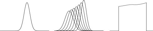
Figure 2: “Flat” marginal $Q(\xi)$ realized by (5) is compared to the marginal $Q_{\beta}(\xi)$ of the exponential family (4). Left $Q_{\beta}(\xi)$ with a fixed value of $\beta$. Center a series of $Q_{\beta}(\xi)$ with $(\beta_{1},\beta_{2},\ldots,\beta_{7})$ are printed over one another. Right $Q(\xi)$ realized by a multicanonical weight defined in (5); a case where $\tilde{P}(\xi)\simeq P(\xi)$ is shown, while it becomes completely flat when $\tilde{P}(\xi)=P(\xi)$. In some cases, behaviors very different from these are observed; see Sec. A.2.

2.2.2 MCMC Sampling with a Multicanonical Weight

So far, we discuss a rather obvious conclusion, but it is more interesting to consider an MCMC simulation that samples the corresponding distribution $Q(x)=G(\xi(x))P(x)/C$. To uniformly cover the region $[\xi_{\min},\xi_{\max}]$, the sample path moves randomly in the region. In other words, the multicanonical weight realizes a random walk on the axis of the target statistics $\xi$; this walk has a memory because the value of $X$ does not determined uniquely by $\xi(X)$.

This behavior enables us to obtain the desired properties using a single chain, as shown in Fig. 3. First, efficient sampling of a tail region with a large value of $\xi$ is possible if we choose a sufficiently large $\xi_{\max}$. On the other hand, fast mixing of MCMC is attained if we choose $\xi_{\min}$ such that the set defined by $\xi_{\min}\leq\xi(x)$ is tightly connected and a sample path can easily move around in it  . Therefore, MCMC sampling with a multicanonical weight shares an “annealing” property with replica exchange MCMC.

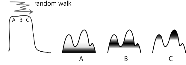
Figure 3: Random walk of $\xi(X)$ realized by a multicanonical weight. Left $P(\xi)$ and a sample path of the random walk projected on the axis of the target statistics $\xi$. Note that the statistics $\xi$ is a function of state $X$, and MCMC updates of $X$ naturally cause such a walk of $\xi$; no separate procedure is required for changing $\xi$. Right A, B, and C show the distributions of $(X,\xi(X))$, each of which corresponds to the regions A, B, and C in the left panel. The vertical axis corresponds to the value of $\xi$, whereas the horizontal axis for each sub-chart schematically represents the high-dimensional space where $X$ takes its value.

Finally, we confirm how probabilities of rare events are computed under the original distribution $P$. We assume that $X^{(i)},i=1,\ldots,M$ are samples from $Q$ defined by $G$ of the equation (5). Then, the following expression is derived from (1):

$$P(\xi_{0}\leq\xi(X)\leq\xi_{\max})\,\simeq\,C\times\frac{1}{M}\sum_{i=1}^{M}\left[\tilde{P}(\xi(X^{(i)}))\,I(\xi_{0}\leq\xi(X^{(i)}))\right],$$

where $I$ is defined by (2). Because the values of $\xi$ are limited in $\xi_{\min}\leq\xi\leq\xi_{\max}$ by our definition of the multicanonical weight,

$$P(\xi_{\min}\leq\xi(X)\leq\xi_{\max})\simeq C\times\frac{1}{M}\sum_{i=1}^{M}\tilde{P}(\xi(X^{(i)})),$$

also holds. Hence, we arrive at

$$\frac{P(\xi_{0}\leq\xi(X)\leq\xi_{\max})}{P(\xi_{\min}\leq\xi(X)\leq\xi_{\max})}\simeq\frac{\sum_{i=1}^{M}\left[\tilde{P}(\xi(X^{(i)}))\,I(\xi_{0}\leq\xi(X^{(i)}))\right]}{\sum_{i=1}^{M}\tilde{P}(\xi(X^{(i)}))}.$$ (6)

The value of the denominator $P(\xi_{\min}\leq\xi(X)\leq\xi_{\max})$ becomes almost unity when the interval $[\xi_{\min},\xi_{\max}]$ contains most of the probability mass; otherwise, in some cases, we are mainly interested in relative probabilities. The expectation of arbitrary statistics $A$ in the tail region $\xi_{0}\leq\xi(x)\leq\xi_{\max}$ is also derived from (3) in a similar manner as

$${\mathbb{E}}[A(X)\,|\,\xi_{0}\leq\xi(X)\leq\xi_{\max}]\simeq\frac{\sum_{i=1}^{M}\left[A(X^{(i)})\,\tilde{P}(\xi(X^{(i)}))\,I(\xi_{0}\leq\xi(X^{(i)}))\right]}{\sum_{i=1}^{M}\left[\tilde{P}(\xi(X^{(i)}))\,I(\xi_{0}\leq\xi(X^{(i)}))\right]}.$$ (7)

2.2.3 Entropic Sampling

Now, we return to the following problem. How to estimate the multicanonical weight $G(\xi)$ in (5) without prior knowledge? The key idea is to use adaptive Monte Carlo; “preliminary runs” of MCMC are repeated to tune the weight $G(\xi)$ until the marginal distribution $Q(\xi)$ becomes almost flat in the interval $[\xi_{\min},\xi_{\max}]$. After tuning the weight, a “production run” is performed, where $G(\xi)$ is fixed; this run realizes MCMC sampling with a multicanonical weight. Note that virtually any type of MCMC can be used for sampling in both of these stages.

An important point is that $G(\xi)$ is a univariate function of a scalar variable $\xi$, while $Q(x)=G(\xi(x))P(x)/C$ is defined on a high-dimensional space of $x$; thus, tuning $G(\xi)$ is much easier than performing a direct adaptation of $Q(x)$ itself.

To illustrate the principle, we describe a simple method, sometimes known as entropic sampling (Lee (1993)). First, we consider the histogram $H$ of the values of $\xi$. It is convenient to introduce a discretized or binned version $\tilde{\xi}(x)$ of $\xi(x)$, which takes an integer value $\tilde{\xi}\in\{1,2,\ldots,N_{b}\}$ .

Then, the histogram of the values of $\tilde{\xi}$ in the $k$th iteration of the preliminary runs is represented by $\{H^{(k)}(\tilde{\xi})\},\tilde{\xi}=1,\ldots,N_{b}$. We define $\bar{H}$ as expected counts in each bin of a flat histogram, which is the target of our adaptation . Further, the weight in the $k$th iteration is represented by $\{G^{(k)}(\tilde{\xi})\},\tilde{\xi}=1,\ldots,N_{b}$. Now that the adaptation in the $k$th step is expressed as a recursion

$$G^{(k+1)}(\tilde{\xi})=G^{(k)}(\tilde{\xi})\times\frac{\bar{H}\,+\,\epsilon}{H^{(k)}(\tilde{\xi})+\epsilon}.$$ (8)

Here, a constant $\epsilon$ is required for eliminating the divergence at $H^{(k)}=0$, which is set to a small value, say, unity. The idea behind this recursion is simple—increase the weight if the counts are smaller than $\bar{H}$ and decrease the weight if the counts are larger than $\bar{H}$.

The tuning stage of the algorithm is formally described as follows. Here, we use $LG(\tilde{\xi})=\log G(\tilde{\xi})$ instead of $G(\tilde{\xi})$.

1. Initialize $LG$ and set parameters.

   • Set $LG(i)=0$ for $i=1,\ldots,N_{b}$.

   • Set the maximum number of iterations $K_{\max}$.

   • Set the number of MCMC steps $M_{\max}$ within each iteration.

   • Set the number of MCMC steps $M_{s}$ between histogram updates.

   • Set a regularization parameter $\epsilon$ (e.g., $\epsilon=1$).

   • Set $\bar{H}=(M_{\max}/M_{s})/N_{b}$.

   • Set the counter of iterations $K$ to $0$.

2. Initialize $H$ and $X$.

   • Set $H(i)=0$ for $i=1,\ldots,N_{b}$.

   • Initialize the state $X$.

   • Set the counter of MCMC trials $M$ to $0$.

3. Run MCMC.

   • Run $M_{s}$ steps of MCMC with the weight $P(x)\exp[LG(\tilde{\xi}(x))]$.

4. Update the histogram $H$.

   • $H(\tilde{\xi}(x^{*}))=H(\tilde{\xi}(x^{*}))+1$, where $X=x^{*}$ is the current state. $\spadesuit$

   • $M=M+M_{s}$.

   • If $M<M_{\max}$, go to Step • ‣ 3.

5. Check whether $H$ is “sufficiently flat.”

   • If so, end.

   • If not and $K<K_{\max}$, modify $LG$.

     • $LG(i)=LG(i)+\log[(\epsilon+\bar{H})/(\epsilon+H({i)})]$ for $i=1,\ldots,N_{b}$. $\clubsuit$

     • $K=K+1$.

     • Go to Step • ‣ 2.

   • If not and $K_{\max}\leq K$, the algorithm fails.

Note that the update formula (8) is included as a step marked with $\clubsuit$, while the histogram is incremented in the step marked with $\spadesuit$.

After completing the above procedure, the production run is performed. If the above algorithm fails to converge, we can increase the numbers $M_{\max}$ and/or $K_{\max}$. Another choice is to reduce our requirement and decrease the value of $\xi_{0}$, which determines the rareness of the obtained events.

The construction of the histogram can be replaced by other density estimation techniques. In the original studies (Berg and Neuhaus (1991, 1992); Berg and Celik (1992)), $\log G(\xi)$ is represented by a piecewise linear curve, instead of a piecewise constant curve used in entropic sampling; parametric curve fitting is also utilized. Another useful method is kernel density estimation, which is particularly convenient in continuous and/or multivariate $\xi$ cases; it is also used with the Wang–Landau algorithm explained later, as seen in Zhou et al (2006). Finally, we mention methods based on the broad histogram equation. In these methods, the number of transitions between states are used for optimizing the weight, instead of the number of visits to a state. Such an idea has a somewhat different origin (de Oliveira et al (1998)), but it can be interpreted as a way to realize a multicanonical weight; see Wang and Swendsen (2002).

2.2.4 Wang–Landau algorithm

Entropic sampling is already sufficient for realizing a multicanonical weight in many problems. In current studies, however, the Wang–Landau algorithm (Wang and Landau (2001b, a)) is often utilized, which provides a more efficient strategy to construct a multicanonical weight.

An essential feature of the Wang–Landau algorithm is the use of a time-inhomogeneous chain in the preliminary runs; that is to say, we change the weights after each trial of MCMC moves instead of changing them only at the end of each iteration consisting of a fixed number of MCMC steps. This may lead to an “incorrect” MCMC sampling in the preliminary runs, but it causes no problem if we fix the weights in the final production run, where we compute the required probabilities and expectations.

In the actual implementation, whenever a state $x$ with $\tilde{\xi}^{*}=\tilde{\xi}(x)$ appears, we multiply the value of weight $G(\tilde{\xi}^{*})$ by a constant factor $0<C<1$ ; it reduces the weights of the already visited values of $\tilde{\xi}$, whereas it effectively increases the relative weights of the other values of $\tilde{\xi}$. In parallel, we construct the histogram $H$ of $\tilde{\xi}$ that appeared in MCMC sampling. After some steps of MCMC, we reach a “sufficiently flat” histogram ; then, a step of iterative tuning of the weights is completed.

When we rerun MCMC where the weight is fixed to the values obtained by this procedure, the run usually does not provide a sufficiently flat histogram of $\tilde{\xi}$. Then, an iterative method is introduced, that is, we increase the value of the constant $C$ and repeat the procedure in the preceding paragraph. A heuristics proposed in the original papers (Wang and Landau (2001b, a)) is to change $C$ to $\sqrt{C}$. After each iteration step, the histogram $H$ is cleared, whereas the values of $G$ are retained.

Again, we stress that any type of MCMC can be used for sampling at each of these stages; we use the familiar Metropolis–Hasting algorithms in the examples considered in this paper. As shown in later sections, however, the choice of moves in the Metropolis–Hasting algorithms significantly affects the efficiency of the entire algorithm.

The tuning of the weight by the Wang–Landau algorithm is summarized as shown below. Again, we use $LG(\tilde{\xi})=\log G(\tilde{\xi})$ in place of $G(\tilde{\xi})$; further, we define $LC=-\log C$ (i.e., with a minus sign).

1. Initialize $LG$ and $LC$; set other parameters.

   • Set $LG(i)=0$ for $i=1,\ldots,N_{b}$.

   • Set $LC>0$ (e.g., $LC=-\log(1/e)=1$).

   • Set the maximum number of iterations $K_{\max}$ (e.g., $K_{\max}\!\!=15$ or $18$).

   • Set the maximum number of MCMC steps $M_{\max}$ within each iteration.

   • Set the counter of iterations $K$ to $0$.

2. Initialize $H$ and $X$.

   • If $K>K_{\max}$, end.

   • Set $H(i)=0$ for $i=1,\ldots,N_{b}$.

   • Initialize the state $X$.

   • Set the counter of MCMC trials $M$ to $0$.

3. Run MCMC.

   • Run a step of MCMC with the weight $P(x)\exp(LG(\tilde{\xi}(x)))$.

4. Modify $LG$ and update the histogram $H$.

   • $LG(\tilde{\xi}(x^{*}))=LG(\tilde{\xi}(x^{*}))-LC$, where $X=x^{*}$ is the current state. $\clubsuit$

   • $H(\tilde{\xi}(x^{*}))=H(\tilde{\xi}(x^{*}))+1$, where $X=x^{*}$ is the current state. $\spadesuit$

5. Check whether $H$ is “sufficiently flat.” 

   • If so, $LC=LC/2$, $K=K+1$ and go to Step • ‣ 2

   • If not and $M<M_{\max}$, $M=M+1$ and go to Step • ‣ 3.

   • If not and $M_{\max}\leq M$, the algorithm fails.

Note that update $\clubsuit$ of the weight $G$ and increment $\spadesuit$ of the histogram $H$ are done simultaneously, in contrast to entropic sampling.

The criterion for a “sufficiently flat” histogram used in Secs. 3.1.1 and 3.1.2 is that counts in every bin of the histogram are larger than 92% of the value expected in a perfectly flat histogram. In the cases of Sec. 3.1.2, we exclude “permanently” zero count bins from the criterion, where true probability seems zero; it is usually difficult to know a priori and some trial and error is required.

After completing the above procedure, the production run is performed. If this algorithm does not converge or the production run using the obtained weights does not give a flat histogram of $\xi$, what can we do? One possibility is to change the criterion that the histogram $H$ is “sufficiently flat;” when we make it more strict and increase the value of $M_{\max}$, convergence may be attained with increasing computational time. Increasing the value of $K_{\max}$ may not be effective when we use the original $\sqrt{C}$ rule for modifying $C$ because the value of $C$ becomes nearly unity for large $K$. Another possibility is to relax our requirement on the rareness and decrease the value of $\xi_{0}$.

The algorithm presented here still contains a number of ad hoc procedures and should be manually adapted to a specific problem. It, however, provides solutions to problems otherwise difficult to treat. On the other hand, many modifications of the algorithm are proposed. Examples of treating continuous variables are seen in Yan et al (2002); Shell et al (2002); Liang (2005); Zhou et al (2006); Atchadé and Liu (2010). The following authors have criticized the $\sqrt{C}$ rule and have proposed modified algorithms: Belardinelli and Pereyra (2007b, a); Liang et al (2007); Zhou and Su (2008); Atchadé and Liu (2010). The convergence of the algorithms is analyzed in Lee et al (2006); Belardinelli and Pereyra (2007b), while rigorous mathematical proofs are discussed in Atchadé and Liu (2010); Jacob and Ryder (2011); Fort et al (2012). Bornn et al (2013) proposed an automatic procedure including the adaptation of step and bin size.

2.2.5 Variance of Estimators

Finally, we will briefly discuss the variance of the estimators. Here, we restrict ourselves to the final production run with a fixed weight. An experimental study on convergence of estimates is shown in Sec. 3.1.1.

At first, we assume that all samples are independent, although it is not true for samples generated by MCMC. Then, variances of the numerator and denominator of the right-hand side of (6) are estimated as

$$\sigma_{m}^{2}=\frac{1}{M}\left\{\sum_{\xi=\xi_{0}}^{\xi_{\max}}\tilde{P}(\xi)\,P(\xi)-\left[P(\xi_{0}\leq\xi)\right]^{2}\right\}$$ (9)

$$\sigma_{m0}^{2}=\frac{1}{M}\left\{\sum_{\xi=\xi_{\min}}^{\xi_{\max}}\!\!\!\tilde{P}(\xi)\,P(\xi)-\left[P(\xi_{\min}\leq\xi\leq\xi_{\max})\right]^{2}\right\}.$$ (10)

From (9) and (10), the relative variance of the right-hand side of (6) is estimated as 

$$\frac{\sigma_{m}^{2}}{[P(\xi_{0}\leq\xi)]^{2}}+\frac{\sigma_{m0}^{2}}{[P(\xi_{\min}\leq\xi\leq\xi_{\max})]^{2}}.$$ (11)

In the case of MCMC, sample correlation becomes important and we should modify these formulae. Let us define integrated auto correlation of statistics $B(X)$ as

$$\mathcal{T}_{B}=\frac{1}{\sigma^{2}_{B}}\sum_{\tau=1}^{\infty}\left\{\mathbb{E_{\mathrm{path}}}[\,B(X^{(0)})\,B(X^{(\tau)})\,]-\mathbb{E}[\,B(X)\,]^{2}\right\},$$

where the expectation $\mathbb{E_{\mathrm{path}}}$ indicates an average over sample paths $X^{(0)},X^{(1)},\ldots$ generated by MCMC, and $\sigma^{2}_{B}$ is the variance of independent samples from the same distribution. Then, the effective number of samples changes from $M$ to $M/\mathcal{T}_{B}$, when we calculate the average of $B$. If we define $\mathcal{T}_{m}$ and $\mathcal{T}_{m0}$ as $\mathcal{T}_{B}$ with $B(X)=\tilde{P}(\xi(X))\,I(\xi_{0}\leq\xi(X))$ and $\tilde{P}(\xi(X))$, respectively, (11) is substituted for

$$\frac{(1+2\mathcal{T}_{m})\sigma_{m}^{2}}{[P(\xi_{0}\leq\xi)]^{2}}+\frac{(1+2\mathcal{T}_{m0})\sigma_{m0}^{2}}{[P(\xi_{\min}\leq\xi\leq\xi_{\max})]^{2}}.$$ (12)

Unfortunately, it is rarely possible to estimate $\mathcal{T}_{m}$ and $\mathcal{T}_{m0}$ a priori. Expression (12), however, suggests that variances $\sigma_{m}^{2}$, $\sigma_{m0}^{2}$ of independent samples and integrated auto correlations $\mathcal{T}_{m}$, $\mathcal{T}_{m0}$ are both important in rare event sampling using MCMC. The multicanonical weight provides a practical method for balancing them.

If correlation among samples is ignored, a reasonable choice of $Q$ for sampling from ${\cal A}=\{x\,|\,\xi_{0}\leq\xi(x)\}$ is $Q_{*}(x)=\tilde{C}P(x)I(\xi_{0}\leq\xi(x))$, which corresponds to the generation of samples using MCMC from the tail $\xi_{0}\leq\xi(x)$ of the distribution $P$. It is, however, not useful in most practical problems, because it is difficult to design a Markov chain that efficiently samples from $Q_{*}(x)$ .

3 Examples of Rare Event Sampling by Multicanonical MCMC

Here, we discuss two applications of multicanonical MCMC, rare event sampling in random matrices and chaotic dynamical systems. Other applications in physics, engineering, and statistics are briefly surveyed.

3.1 Rare Events in Random Matrices

A pioneering study on rare events in random matrices with multicanonical MCMC is Driscoll and Maki (2007), which computes large deviation in growth ratio, a quantity relevant to the numerical difficulty in treating matrices. The results in this subsection are discussed in detail in Saito et al (2010) and Saito and Iba (2011). Kumar (2013) also applied the Wang-Landau algorithm to random matrices using coulomb gas formulation.

3.1.1 Largest Eigenvalue

Distributions of the largest eigenvalue $\lambda^{\max}$ of random matrices are of considerable interest in statistics, ecology, cosmology, physics, and engineering. Small deviations have been studied in this problem, and have yielded the celebrated $N^{1/6}$ law by Tracy and Widom (1994, 1996). Here, we are interested in the numerical estimation of large deviations; the present analytical approach to large deviations is limited to specific types of distributions (Dean and Majumdar (2008); Majumdar and Vergassola (2009)). Specifically, the probability $P(\lambda^{\max}<0)$ that all eigenvalues are negative is important in many examples, because it is often related to the stability of the corresponding systems (May (1972); Aazami and Easther (2006)).

In Saito et al (2010), multicanonical MCMC is applied to this problem. Rare events whose probability $P(\lambda^{\max}<0)$ is as small as $10^{-200}$ are successfully sampled for matrices of size $N\leq 30$ (or $40$) .

Examples of the results in Saito et al (2010) are shown in Figs. 4 and 5. In Fig. 4, the probability $P(\lambda^{\max}_{0}<\,\lambda^{\max}\!\leq\lambda^{\max}_{0}\!+\delta)$ is plotted against the values of $\lambda^{\max}_{0}$ with a small binsize $\delta$ for the case of Gaussian orthogonal ensemble (GOE). GOE is defined as an ensemble of random real symmetric matrices such that entries are independent Gaussian variables; hereafter, the variances of the diagonal and off-diagonal components are 1 and 0.5, respectively, while means are all zero.

Fig. 5 shows the probability $P(\lambda^{\max}<0)$ that all eigenvalues are negative. The results for GOE and an ensemble of real symmetric matrices whose components are uniformly distributed (hereafter “uniform”) are shown . For small $N$s, the results from the proposed method reproduce those by simple random sampling . On the other hand, for a large $N$ for which simple random sampling hardly suffices, the obtained results match theoretical results in the case of GOE. The typical number of steps in preparing the multicanonical weight is $2\sim 5\times 10^{9}$, and the length of the final productive run ranges from $1\times 10^{9}$ (GOE $N=20$) to $2.5\times 10^{9}$ (GOE $N=40$, uniform $N=30$) .

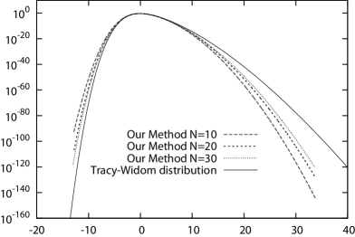
Figure 4: The probability $P(\lambda^{\max}_{0}<\,\lambda^{\max}\!\leq\lambda^{\max}_{0}\!+\delta)$ estimated by the proposed method is plotted for $N=10,20$, and $30$, where $\delta$ is a small binsize. The Tracy–Widom distribution for small deviation asymptotics is shown by the solid curve; systematic deviations from the obtained result for large deviation are observed as expected. The horizontal axis corresponds to the scaled variable $(\,\lambda^{\max}_{0}-\mathbb{E}(\lambda^{\max}_{0})\,)N^{1/6}$. Gaussian orthogonal ensemble (GOE) is assumed. [from N. Saito, Y. Iba, and K. Hukushima, Multicanonical sampling of rare events in random matrices, Physical Review E 82, 031142 (2010), © 2010 American Physical Society]

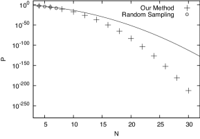
Figure 5: Probabilities $P(\lambda^{\max}<0)$ obtained by the proposed method and simple random sampling method are shown against $N$; the latter is available only for small $N$. Left GOE; curve indicates a quadratic fit to the results with Coulomb gas representation (Dean and Majumdar (2008)). Right an ensemble of matrices whose components are uniformly distributed; curve indicates the probability for GOE with the same variance. [from N. Saito, Y. Iba, and K. Hukushima, Multicanonical sampling of rare events in random matrices, Physical Review E 82, 031142 (2010), © 2010 American Physical Society]

Examples of convergence of estimates are shown in Fig. 6. For an ensemble of matrices whose components are uniformly distributed, multicanonical weights for $N=6,12,18$ and $24$ are calculated by the Wang–Landau algorithm using at most $5.0\times 10^{9}$ steps. Then, five independent production runs are performed for each $N$ using the same weight obtained by this procedure. The results for an increasing length of the production run are shown in the figure. Noting that the vertical axis of Fig. 5 is log-scale, the variance of the estimates attained in Fig. 6 is reasonably small and is enough for providing an accurate test for asymptotics.

Figure 6: Examples of the convergence of estimated probabilities. Upper Left $N=6$, Upper Right $N=12$, Lower Left $N=18$, and Lower Right $N=24$. The vertical axis corresponds to probabilities $P(\lambda^{\max}<0)$, while the horizontal axis (log-scale) corresponds to the steps of the algorithm. Results of five production runs with the same weight and different random numbers are shown for each $N$; in the $N=6$ case, symbols are almost overlapped one another. An ensemble of matrices whose components are uniformly distributed is assumed.

The proposed method is quite general and can be applied to random matrices whose components are sampled from an arbitrary distribution, or even random sparse matrices, to which no analytical solution is available. These results are discussed in detail in Saito et al (2010), along with the detailed specifics of the proposed algorithm.

An important lesson from this example is that we should be careful while choosing the moves in the Metropolis–Hasting algorithm. If we generate candidates using conditional distributions of the original distribution, such as the Gaussian distribution for each component in GOE, the algorithm fails in some cases. This occurs because such a method cannot generate candidates with very large deviations in a component. This difficulty is avoided by the use of a random walk Metropolis algorithm with an adequate step size; in the example of GOE, we use Gaussian distributions as proposal distributions in the Metropolis algorithm (variances are unity for diagonals and 0.5 for non diagonals, respectively); see Saito et al (2010).

3.1.2 Random Graphs

The search for rare events in random graphs is also an interesting subject. An undirected graph is represented by the corresponding adjacency matrix, whose components take values in the set $\{0,1\}$. For a k-regular graph, the maximum eigenvalue takes a fixed value equal to $k$, and hence it is not interesting. On the other hand, the spectral gap $\lambda^{\rm gap}$, given as the difference between the maximum and the second-largest eigenvalue in the case of regular graphs, is related to many important properties of the corresponding graph. Specifically, graphs with larger values of the spectral gap are called Ramanujan graphs or expanders; Ramanujan graphs have interesting properties for communications and dynamics on networks (see references in Donetti et al (2006); Saito and Iba (2011)).

In earlier studies, Donetti et al (2005, 2006) optimized the spectral gaps of graphs by simulated annealing; in their algorithm, a pair of edges of the graph is modified in each Metropolis–Hasting step. Using this method, they showed that expanders with interesting structures automatically appear.

Saito and Iba (2011) applied multicanonical MCMC to this problem; they defined the Metropolis-Hasting update as in Donetti et al (2005, 2006) and used the Wang–Landau algorithm for realizing multicanonical weights. Examples of the obtained graphs are shown in Fig. 7, while Fig. 8 gives probability $P(\lambda^{\rm gap}_{0}<\lambda^{\rm gap})$ as a function of $\lambda^{\rm gap}_{0}$ and the size $N$ of matrices. The typical number of Metropolis steps used in preparing multicanonical weights is $0.5\sim 1.0\times 10^{9}$, while the length of the final production run is $0.25\sim 0.5\times 10^{9}$. See Saito and Iba (2011) for further details.

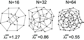
Figure 7: Examples of 3-regular graphs with a large spectral gap found in the simulation. [from N. Saito and Y. Iba, Probability of graphs with large spectral gap by multicanonical Monte Carlo, Computer Physics Communications 182 223-225 (2011), © 2011 Elsevier]

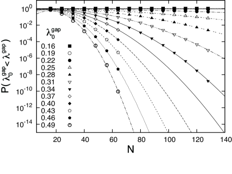
Figure 8: Estimated $P(\lambda^{\rm gap}_{0}<\lambda^{\rm gap})$ are shown as functions of $N$. Each curve corresponds to different values of $\lambda^{\rm gap}_{0}$. Data are well fitted by quadratic functions when $\lambda^{\rm gap}_{0}\gtrsim 0.18$. [from N. Saito and Y. Iba, Probability of graphs with large spectral gap by multicanonical Monte Carlo, Computer Physics Communications 182 223-225 (2011), © 2011 Elsevier]

3.2 Rare Events in Dynamical Systems

Rare events in deterministic dynamical systems are important both in theory and application (Ott (2002); Beck and Schlögl (1993)). An example is a quantitative study on tiny tori embedded in a “chaotic sea” of Hamiltonian dynamical systems, which is a familiar subject in this field. Numerical effort required for uncovering these tiny structures dramatically increases with the dimension of the system. Therefore, it is natural to introduce MCMC and other stochastic sampling methods to this field. Studies on MCMC search for unstable structures in dynamical systems are found in Sasa and Hayashi (2006); Yanagita and Iba (2009); Geiger and Dellago (2010), and references therein .

Kitajima and Iba (2011) applied multicanonical MCMC to the study of dynamical systems. In the proposed algorithm, a measure of the chaoticity of a trajectory is defined as a function of the initial condition , which corresponds to statistics representing rareness. Then, the Metropolis–Hastings update is defined as follows: (1) perturb the initial condition, (2) simulate a fragment of trajectory from the new initial condition, and (3) calculate the chaoticity of the trajectory and reject/accept the new initial condition using the current weight. Then, the entire algorithm is defined as multicanonical MCMC with the Wang–Landau algorithm for tuning the weight.

Again, the choice of moves in the Metropolis–Hastings algorithm is important; here, we sample a perturbation to the initial conditions from a mixture of uniform densities with different order of widths. This idea, taken from Sweet et al (2001), seems essential for sampling from fractal-like densities; see Kitajima and Iba (2011) for details.

In Kitajima and Iba (2011), sampling of tiny tori in the chaotic sea of a four-dimensional map

$$u_{n+1} =u_{n}-\frac{K}{2\pi}\sin(2\pi v_{n})+\frac{b}{2\pi}\sin(2\pi(v_{n}+y_{n}))$$

$$v_{n+1} =v_{n}+u_{n+1}$$

$$x_{n+1} =x_{n}-\frac{K}{2\pi}\sin(2\pi y_{n})+\frac{b}{2\pi}\sin(2\pi(v_{n}+y_{n}))$$

$$y_{n+1} =y_{n}+x_{n+1}$$

is studied, where $K$ and $b$ are constants that characterize the map. An example of tiny tori found by the proposed method is shown in Fig. 9. In this case, the total number of initial conditions tested in the proposed algorithm is about $4\times 10^{9}$, while the probability to find an initial configuration leading to a trajectory with the same degree of chaoticity is as small as $10^{-12}$, assuming random sampling from the Lebesgue measure. In addition, the relative volume of initial conditions that lead to trajectories of the given order of “chaoticity” are successfully estimated by the algorithm; that is, the proposed method is not only useful for the search but also provides quantitative information on rare events in dynamical systems, see Fig. 2 of Kitajima and Iba (2011).

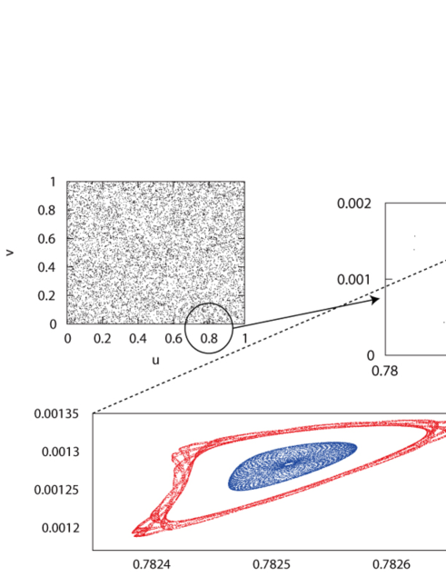
Figure 9: Pair of tiny tori in the chaotic sea found by the proposed method. Projections on the $(u_{n},v_{n})$-plane are shown. Enlargement of a tiny area in the small circle in the left panel is given in the right panel; further enlargement is given in the lower panel. $K=7.8$ and $b=0.001$. [from A. Kitajima and Y. Iba, Multicanonical sampling of rare trajectories in chaotic dynamical systems, Computer Physics Communications 182 251-253 (2011), © 2011 Elsevier]

3.3 Other Applications

The rest of this section briefly describes other fields of applications of multicanonical MCMC.

3.3.1 Statistical Physics

Multicanonical MCMC was originally developed for sampling from Gibbs distributions in statistical physics. Hence, a number of studies in this field have successfully applied it to problems where simple MCMC is virtually disabled by slow mixing. Some typical examples are studies on the Potts and other classical spin models (Berg and Neuhaus (1992); Wang and Landau (2001a); Zhou et al (2006)), spin glass models (Berg and Celik (1992); Wang and Landau (2001a)), and liquid models (Yan et al (2002); Shell et al (2002); Calvo (2002)). Multicanonical MCMC is also used for the study of biomolecules (see Mitsutake et al (2001); Higo et al (2012) for full-atom protein models and Chikenji et al (1999); Wüst and Landau (2012) for lattice protein models). Attempts to combine the idea of multicanonical weight with chain growth algorithms are found in Bachmann and Janke (2003); Prellberg and Krawczyk (2004). More examples are found in the review articles mentioned in Sec.1.

On the other hand, the use of multicanonical MCMC for other types of rare event sampling in physics is a recent challenge . Hartmann (2002) introduced the idea of rare event sampling by MCMC to the physics community. Körner et al (2006) and Monthus and Garel (2006) applied MCMC to the sampling of disorder configurations that gives large deviations in ground state energies; in these studies, modifications of the Gumbel distribution are used for approximating multicanonical weights. Subsequently, Hukushima and Iba (2008) and Matsuda et al (2008) applied the Wang–Landau algorithm to the study of Griffiths singularities in random magnets, which is known to be sensitive to rare configurations of impurities; Wolfsheimer and Hartmann (2010) discussed RNA secondary structures. In these studies, any prior knowledge on the functional form of $\tilde{P}(\xi)$ is assumed.

3.3.2 Optical Telecommunication and Related fields

Multicanonical MCMC is intensively used for rare event sampling in optical telecommunication and related fields. After a pioneering work by Yevick (2002), a number of applications appeared; see, for example, Holzlöhner and Menyuk (2003), and a recent review, Bononi et al (2009). The sampling of rare noises that cause failures of error correction is discussed in Holzlöhner et al (2005) and Iba and Hukushima (2008), which can be useful for predicting the performance of error-correcting codes.

3.3.3 Statistics

Algorithms based on the multicanonical weight, specifically, the Wang–Landau algorithm and its generalizations, increasingly attract the attention of statisticians. Liang (2005) introduced the Wang–Landau algorithm to statistics. Atchadé and Liu (2010) and Chopin et al (2012) developed closely related algorithms and tested them in examples of Bayesian inference and model selection. Bornn et al (2013) and Kastner et al (2013) also discussed applications in Bayesian statistics; Kwon and Lee (2008) treated a target tracking problem. Yu et al (2011) (also Liang et al (2010)) discussed hypothesis testing using stochastic approximation Monte Carlo. Wolfsheimer et al (2011) extended the study of Hartmann (2002) and applied rare event sampling using the Wang-Landau method to the computation of p-values for local sequence alignment problems. 5. Add the following reference to the reference lis In the following section, we will discuss exact tests and data surrogation as an application field of multicanonical MCMC for constrained systems.

4 Sampling from Constrained Systems and Hypothesis Testing

Sampling from highly constrained systems and combinatorial calculations are discussed here as a variation of the theme of rare event sampling. Exact tests and data surrogation are introduced as an application field of this idea, where efficient sampling from constrained systems is essential.

For general issues on Monte Carlo approximate counting, see Jerrum and Sinclair (1996), Rubinstein and Kroese (2008), and Rubino and Tuffin (2009).

4.1 MCMC Sampling from Constrained Systems

MCMC sampling is difficult when constraints exist among random variables. In such cases, it is often not easy to find a set of Metropolis–Hastings moves that realizes an ergodic Markov chain without violating the constraints. For example, considerable effort is devoted to find ergodic moves for contingency tables with fixed margins and other constraints (Diaconis and Sturmfels (1998); Bunea and Besag (2000); Takemura and Aoki (2004)) . Although partial success has been obtained using highly sophisticated mathematics, the problem becomes increasingly difficult when problem complexity increases.

Yet another general strategy for dealing with highly constrained systems is an introduction of “soft constraints.” First, given constraints $f_{i}(x)=0$, $i=1,\cdots L$, we define statistics $\xi$ of the state variables $X$ that satisfy the following conditions: (1) $\xi(X)\geq 0$ and (2) $\xi(X)=0$, if and only if $X$ satisfy $f_{i}(X)=0$ for all $i$. A simple example of such statistics is

$$\xi(x)=\sum_{i=1}^{L}c_{i}|f_{i}(x)|^{\alpha}.$$

Here, $\alpha>0$ and $c_{i}>0$ are arbitrary constants; $\alpha=1$ is usually better than $\alpha=2$ because $\xi$ keeps small values when $|f_{i}(x)|$ increases in the case of $\alpha=1$. Then, a finite value of $\xi$ represents soft constraints, whereas $\xi=0$ corresponds to the original hard constraints. Random sampling of the value of $X$ usually gives a large value of $\xi(X)$; hence, $\xi(X)=0$ can be regarded as a “rare event.”

At this point, we introduce multicanonical MCMC with target statistics $\xi$ and sample rare events $X$ defined by $\xi(X)=0$ (or, for a continuous variable $X$, $\xi(X)\approx 0$). Then, after tuning weights with the Wang–Landau algorithm, a production run provides samples of $X$ that (nearly) satisfy the constraints $f_{i}(X)=0$ (or $f_{i}(X)\approx 0$) for all $i$. Note that a similar strategy can be implemented using a combination of an exponential family with sufficient statistics $\xi$ and replica exchange MCMC; in this case, a large value of $\beta$ corresponds to hard constraints.

Some references are as follows . Pinn and Wieczerkowski (1998) introduced replica exchange MCMC with soft constraints to this field, and the number of magic squares of size $6\times 6$ is estimated in their paper. Kitajima and Kikuchi (private communication) extended it to $30\times 30$ using multicanonical MCMC. Hukushima (2002) estimated the number of N-queen configurations by replica exchange MCMC, while Zhang and Ma (2009) treated N-queen and Latin squares using a hybrid of simulated tempering (Sec. A.3) and the Wang–Landau algorithm; they dealt with Latin squares up to size $100\times 100$. Fishman (2012) proposed an approach based on soft constraints for counting contingency tables; conventional MCMC is used in his paper.

4.2 Application to Hypothesis Testing

Here, we discuss how multicanonical MCMC (and also replica exchange MCMC) can be useful for exact tests and data surrogation; the proposed method is tested with a simple example of time series.

4.2.1 MCMC Exact Tests

MCMC is useful for implementing statistical tests with a complicated null distribution. Particularly important cases occur when the null distribution is a distribution conditioned with a set of statistics $\zeta_{i}$. In these cases, the null hypothesis is represented as the uniform distribution of $X$ on the set defined by $\zeta_{i}(x)=\zeta_{i}^{o},\,i=1,\ldots L$, where $X$ is a random variable and $\zeta_{i}^{o}$ is the value of statistics $\zeta_{i}$ corresponding to the observed data. For a continuous variable $X$, this condition can be relaxed as

$$|\zeta_{i}(x)-\zeta_{i}^{o}|<\epsilon_{i},\,i=1,\ldots L,$$ (13)

where $\epsilon_{i}$ is a constant with a small value.

A prototype of such a test is Fisher’s exact test of contingency tables (Agresti (1992)), where the marginals of the table correspond to $\zeta_{i}$’s; a number of extended versions exist and MCMC algorithms with complicated Metropolis moves have been developed for them, as mentioned in the previous section. Besag and Clifford (1989) described a test where an Ising model on the square lattice represents the null hypothesis.

In our view, it is natural to introduce the “soft constraint” strategy described in Sec. 4.1 to this problem. When we define the statistics $\xi$ as $\xi(x)=\sum_{i=1}^{L}|\zeta_{i}(x)-\zeta_{i}^{o}|$, it is straightforward to apply multicanonical MCMC for sampling $X$ that uniformly distributed on the set defined by $\zeta_{i}(x)=\zeta_{i}^{o},\,i=1,\ldots L$ or its generalization (13). This strategy is quite general and can be applied to a variety of MCMC hypothesis testing .

4.2.2 Data Surrogation

In nonlinear dynamics and neural science, statistical tests for time series based on (13) are well developed (Schreiber and Schmitz (2000)). They are called as surrogate data methods, and samples from null distributions defined by (13) are called as surrogates of the original data. An example of the problem where surrogation is intensively used is testing of statistical properties of neural spike trains (Grün and Rotter (2010)).

In conventional approaches, surrogates are generated by partial randomization of the original data. For example, if the phase of time series data $x^{o}(t),t=1,\ldots,N$ is randomized after the complex Fourier transform, then its inverse transform $x=\{x(t)\}$ has the same sets of correlation functions

$$C(x;\tau)=\sum_{t=1}^{N-\tau}x(t)x(t+\tau)$$ (14)

as the original time series  and is considered as a surrogate that maintains the value of sufficient statistics $\zeta_{\tau}(x)=C(x;\tau)$. Although a quick solution is provided in this case, solutions to general cases are only found on a case-by-case basis, and it becomes increasingly difficult as the complexity of the problems increases.

Therefore, Schreiber proposed a general idea of regarding data surrogation as an optimization problem (Schreiber (1998); Schreiber and Schmitz (2000)). According to this idea, generating a surrogate is equivalent to finding a solution of (13), which can be treated by a general-purpose optimization algorithm, for example, simulated annealing. An application of this idea in neural science is found in Hirata et al (2008).

This was an epoch-making idea in this field; randomization via a clever idea was no longer required, being replaced by a routine procedure at the cost of computational time. However, in data surrogation, we want to generate a sample (or a set of samples) unbiasedly selected from the null distribution defined by (13), and not obtain a sample that satisfies (13).

Therefore, applying multicanonical MCMC seems a better choice. Hence, we again arrive at the idea of exact testing with multicanonical MCMC.

4.2.3 Example

Let us illustrate the idea of “multicanonical surrogation” using an example from Schreiber (1998)  . In this example, the problem is to generate artificial time series $x=\{x_{1},x_{2},\ldots,x_{N}\}$ by permuting the original time series $x^{o}=\{x^{o}_{1},x^{o}_{2},\ldots,x^{o}_{N}\}$ given as observed data. The constraint is to maintain the correlation functions $C(x;\tau)$, defined as (14), to be nearly equal to the original correlation functions $C(x^{o};\tau)$ for $\tau=1\ldots T$; here, the constant $0<T<N$ is the maximum of the delay $\tau$, where we expect correlation coincidence.

Here, $\xi(X)=\sum_{\tau=1}^{T}\left|C(X;\tau)-C(x^{o};\tau)\right|$ is used to define multicanonical MCMC that samples $X=\{X_{1},X_{2},\cdots X_{N}\}$. $\xi(X)$ is zero if and only if $C(X;\tau)=C(x^{o};\tau)$ for all $1\leq\tau\leq T$. Then, Metropolis–Hastings moves are defined by the swap of a randomly selected pair. In detail, a pair $i$ and $j$ is selected by a random number in each step and a new candidate $x^{\rm new}$ of $X$ is generated by $x^{\rm new}_{i}=x_{j}$ and $x^{\rm new}_{j}=x_{i}$ without changing other components, using the current values $X_{i}=x_{i}$ and $X_{j}=x_{j}$. Here, the value of $\{X_{i}\}$ is initialized as a random permutation of $\{x_{i}^{o}\}$.

In the following experiment, we consider time series $x^{o}$ of length $N=400$ generated by nonlinear observations of a linear AR process $y$ driven by uniform noise, that is,

$$x_{t}^{o}=y_{t}^{3},\,\,\,y_{t+1}=0.3y_{t}+\eta_{t},\,\,\,\eta_{t}\sim U(-2,2).$$

Here, we choose $T=8$. Multicanonical MCMC is designed for realizing an approximately flat distribution of $\xi$ in the interval $[0,4800.8]$, which is divided into ${80}$ bins . In this choice of the interval, we consider two conditions: (1) the interval contains a high entropy region where the values of $\xi$ are readily realized by a random permutation of the original time series, and (2) the last bin $\xi\simeq 0$ corresponds to a tail region of $\xi$ that we are interested in. The Wang–Landau algorithm with $K_{\mathrm{max}}=15$ is used to tune the weight; the $\sqrt{C}$ rule is utilized. At each step of the iteration, we run MCMC until counts in each bin coincide with the value for the uniform histogram within 1% accuracy. The total number of Metropolis trials is $2.5\times 10^{8}$, of which $3.2\times 10^{7}$ are used for the final production run.

The results of this experiment are shown in Figs. 10 and 11. In Fig. 10, the distribution of $\xi$ realized in the production run and the estimated log-density of $\xi$ are shown. The former is not quite flat in a non-logarithmic scale, but enough to ensure efficient production of the desired samples. According to the right panel of Fig. 10, the probability of obtaining a sample within the bin $\xi\approx 0$ is estimated to be as small as $10^{-25}$ or less, assuming a random permutation of $x^{o}$.

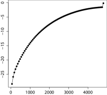
Figure 10: Left frequency of the occurrence of $\xi$ in the production run of multicanonical MCMC. The horizontal and vertical axes correspond to the value of $\xi$ and the observed frequency in the given bins, respectively. Right probability density of $\xi$. The horizontal and vertical axes correspond to the value of $\xi$ and the estimated log-probabilities ($\log_{10}$), respectively; a set of bins used in the left panel is also applied in the right panel for defining probabilities. The spike in the rightmost bin corresponds to a cumulated probability of larger values of $\xi$. [from Y. Iba, IEICE Technical Report IBISML2011-7(2011-06), 43-50, in Japanese, ©IEICE 2011]

In Fig. 11, the quality of the obtained samples is examined. In the left panel, three samples in the last bin $\xi\simeq 0$ are shown, which are considerably different from one another. In the right panel, correlation functions $C(x^{(k)},\tau)$ are calculated for each of the 1976 samples $X=x^{(k)}$, $k=1,\ldots,{1976}$, in the bin $\xi\approx 0$ and compared to the original $C(x^{o},\tau)$, which indicate an extremely good agreement between them .

Figure 11: Left surrogate data generated by the proposed method. Uppermost series correspond to the original data and other three are surrogates. The horizontal and vertical axes correspond to $t$ and $x_{t}$, respectively. Right comparison of correlation functions. The horizontal and vertical axes correspond to the delay $\tau$ and the values of the correlation function, respectively. The line represents $C(x^{o},\tau)$, which corresponds to the original data, while black dots represent sets of $C(x^{(k)},\tau)$ obtained from surrogated data; $N=400$ is the length of the time series. The results of 1976 samples are printed over each other; hence, symbols are almost overlapping. [from Y. Iba, IEICE Technical Report IBISML2011-7(2011-06), 43-50, in Japanese, ©IEICE 2011]

5 Summary and Discussions

In this paper, we discussed rare event sampling using multicanonical MCMC. Two different methods of tuning the weight, entropic sampling and the Wang–Landau algorithm, are explained. Then, examples for random matrices, random graphs, chaotic dynamical systems, and data surrogation are shown. We hope our exposition will be useful for the exploration of further novel applications of multicanonical MCMC.

Appendix A Appendix

A.1 Multicanonical MCMC for Exponential Family

We begin this paper with a history of multicanonical MCMC; it was originally developed as a method for sampling from Gibbs distributions, or an exponential family. Here, we briefly discuss how to use multicanonical MCMC for this original purpose.

Assume that we want to compute the expectation ${\mathbb{E}_{\beta}}[A(X)]=\sum_{x}A(x)\,\exp(\beta\xi(x))/Z_{\beta}$ of statistics $A$ from the output $X^{(i)},i=1,\ldots,M$ obtained from multicanonical MCMC that realizes an almost flat marginal of $\xi$ in a “sufficiently wide” interval $[\xi_{\min},\xi_{\max}]$. Then, for $M\rightarrow\infty$, the desired expectation is computed by the reweighting formula 

$${\mathbb{E}_{\beta}}[A(X)]\simeq\frac{\sum_{i=1}^{M}\left[A(X^{(i)})\,\tilde{P}(\xi(X^{(i)}))\,\exp(\beta\xi(X^{(i)}))\right]}{\sum_{i=1}^{M}\left[\tilde{P}(\xi(X^{(i)}))\,\exp(\beta\xi(X^{(i)}))\right]}.$$ (15)

Further, we have an expression for the normalizing constant $Z_{\beta}$ as

$$\frac{Z_{\beta}}{V}\simeq\frac{\sum_{i=1}^{M}\left[\tilde{P}(\xi(X^{(i)}))\,\exp(\beta\xi(X^{(i)}))\right]}{\sum_{i=1}^{M}\tilde{P}(\xi(X^{(i)}))},$$ (16)

where $V$ is the total number of states of the variable $X$ that satisfy $\xi_{\min}<\xi(X)<\xi_{\max}$; it is useful for the calculation of marginal likelihood in statistics and free energy in physics.

It is easy to derive these expressions  considering that the multicanonical weight is proportional to $\tilde{P}(\xi(X^{(i)}))^{-1}$.  Expressions (15) and (16), however, are quite unusual in the sense that we can use them for a broad range of $\beta$ where the interval $[\xi_{\min},\xi_{\max}]$ covers a necessary region. Using this property, multicanonical MCMC simultaneously gives the expectations ${\mathbb{E}_{\beta}}[A(X)]$ for all $\beta$, through a single production run of a single chain. This is because a multicanonical weight gives a flat distribution of $\xi$ that has a considerable overlap with the distribution $\exp(\beta\xi(x))/Z_{\beta}$ for any value of $\beta$, which is intuitively understood from the left panel in Fig. 12.

If we consider a similar reweighing that uses outputs of MCMC at $\beta^{\prime}$ for computing the expectation at a different $\beta$, it is practically impossible for a high-dimensional $X$ unless the difference $|\beta^{\prime}-\beta|$ is very small. This is because the overlap of the distributions virtually vanishes as shown in the right panel of Fig. 12; in such cases, the variance of summands on the right-hand side of (15) drastically increases.

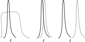
Figure 12: Overlap of marginals of $\xi$. The horizontal axis corresponds to the sufficient statistics $\xi$. Left a multicanonical weight (gray) and a member with a given $\beta$ of the exponential family (black). Central and right panels a pair of members with different values $\beta$ and $\beta^{\prime}$ of the exponential family. The center panel corresponds to cases with a small $|\beta^{\prime}-\beta|$, whereas the right panel corresponds to cases with a large $|\beta^{\prime}-\beta|$.

A.2 First-Order Transition and “Phase Coexistence”

As already mentioned in the main text, there are examples in which a region of $\xi$ is virtually not realized for any choice of the canonical parameter $\beta$ of the exponential family with sufficient statistics $\xi$. The marginal distribution of $\xi$ has multiple peaks in this region of $\beta$, as illustrated in Fig. 13. Such examples naturally appear in statistical physics, when we study the “phase coexistence” phenomena near first-order phase transitions . On the other hand, it seems that the significance of such phenomena in statistics and engineering has not been fully explored.

In such cases, distributions defined by multicanonical weights are not well approximated by a mixture of the members of the corresponding exponential family; this is easily understood by considering Fig. 13. Hence, the advantage of replica exchange MCMC is limited because the sample path is blocked by the gap of $\xi$, while multicanonical MCMC can, in principle, do better. Both methods, however, seem to fail in very difficult cases; see Iba and Takahashi (2005).

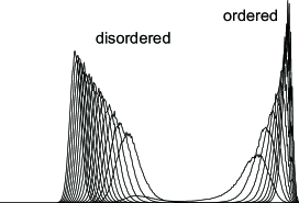
Figure 13: Marginals of $\xi$ with different values of $\beta$ in the case of phase coexistence; the horizontal axis corresponds to the sufficient statistics $\xi$. These curves are obtained from the 10-states Potts model (see Berg and Neuhaus (1992)), which consists of discrete variables $\{X_{i}\},\,X_{i}\in\{1,\cdots,10\}$ on a square lattice; they are computed by reweighting of the outputs of a single production run of multicanonical MCMC. If $\{X_{i}\}$ belongs to an “ordered” component, most $X_{i}$s take the same value. In contrast, their values are almost random in the “disordered” component. In the disordered component, $\xi$ takes smaller values, but the number of states of $X$ that belongs to the component is large; hence, the total probability is comparable in both components.

A.3 Simulated Tempering

The “third” method, simulated tempering (Marinari and Parisi (1992); Geyer and Thompson (1995)), or expanded ensemble Monte Carlo (Lyubartsev et al (1992)) , is briefly explained here. Practically, we recommend choosing between multicanonical MCMC and replica exchange MCMC. Simulated tempering, however, provides an idea that interpolates these two algorithms and is conceptually important. The idea is simple—inverse temperature $\beta$ is regarded as a random variable (hereafter denoted by $\mathpzc{B}$) and we consider MCMC sampling of $(X,\mathpzc{B})$ from the combined distribution

$$P(x,\beta)=\frac{\exp(\beta\xi(x))}{Z_{\beta}}\,\pi(\beta)=\exp(\beta\xi(x)-\log Z_{\beta}+\log\pi(\beta)).$$

Hereafter, we choose a “pseudo prior” $\pi(\beta)$ as a uniform density on $[\beta_{\min},\beta_{\max}]$, resulting in a random walk of $\mathpzc{B}$ that uniformly covers the interval $[\beta_{\min},\beta_{\max}]$; see Fig. 14. This behavior is similar to that of multicanonical MCMC, but here $\mathpzc{B}$ is a variable updated in a separate step of MCMC; in contrast, a random walk of $\xi(X)$ is induced by the update of the state $X$ in case of multicanonical MCMC.

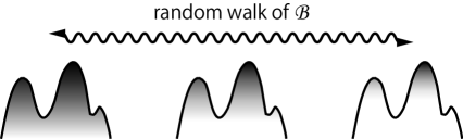
Figure 14: Random walk of inverse temperature variable $\mathpzc{B}$ in simulated tempering. The vertical axis corresponds to the value of $\xi$, whereas the horizontal axis for each sub-chart schematically represents a high-dimensional space of $X$. The values of inverse temperature $\beta$ are assumed to increase from left to right; the shading represents the corresponding changes in high-probability regions. Note that a random variable $\mathpzc{B}$ is updated by MCMC, retaining the value of $X$ at that time; in other words, a separated procedure for changing $\mathpzc{B}$ is required for simulated tempering.

Although this concept is simple, a difficulty arises because the MCMC update of $\mathpzc{B}$ requests the value of $Z_{\beta}$ as a function of $\beta$, which is unknown in most cases . Hence, we should introduce the estimation of $Z_{\beta}$ using repeated preliminary runs, which is similar to the weight tuning procedure in multicanonical MCMC. See the above references, as well as Zhang and Ma (2007), which introduced a method like the Wang–Landau algorithm.

A.4 Implementation on Parallel Hardware

Replica exchange MCMC is naturally parallelizable. Then, how can we efficiently implement multicanonical MCMC on parallel hardware? A simple solution is parallelization of the weight tuning stage. That is, a set of preliminary runs is performed in parallel, each of which runs on a CPU; they share a histogram where total number of visits to each value of $\xi$ is recorded. Some variants of this idea are discussed in, for example, Zhan (2008); Bornn et al (2013). If we want to go beyond these schemes, something more intricate is required. For example, the range of $\xi$ is divided into a set of intervals and a multicanonical weight is realized in each of them; see Wang and Landau (2001a); Mitsutake et al (2001); Vogel et al (2013). In the latter two studies, the exchange of states between neighboring intervals is incorporated.

A.5 Multivariate Extensions

Multicanonical MCMC samples a high-dimensional $X$, while adaptation of the weight is performed in a one-dimensional space of $\xi$. It is possible to introduce a “multivariate multicanonical weight,” which realizes an almost uniform density in a region of two-dimensional $(\xi_{1},\xi_{2})$ or even three-dimensional $(\xi_{1},\xi_{2},\xi_{3})$ spaces, where $\xi_{k}$ is a function of $X$. Examples of such extensions are found in Shteto et al (1997); Iba et al (1998); Higo et al (1997); Chikenji et al (1999); Chikenji and Kikuchi (2000); Yan et al (2002); Zhou et al (2006). Usually, the adaptation of weights in a multivariate case is more difficult than in a univariate case, because of the sparseness of the data collected in the preliminary run; Zhou et al (2006) proposed the use of kernel density estimation for this problem.