The Dynamics of an Electric Dipole Moment in a Stochastic Electric Field

Abstract

The mean-field dynamics of an electric dipole moment in a deterministic and a fluctuating electric field is solved to obtain the average over fluctuations of the dipole moment and the angular momentum as a function of time for a Gaussian white noise stochastic electric field. The components of the average electric dipole moment and the average angular momentum along the deterministic electric field direction do not decay to zero, despite fluctuations in all three components of the electric field. This is in contrast to the decay of the average over fluctuations of a magnetic moment in a stochastic magnetic field with Gaussian white noise in all three components. The components of the average electric dipole moment and the average angular momentum perpendicular to the deterministic electric field direction oscillate with time but decay to zero, and their variance grows with time.

I Introduction

We consider the decoherence of an electric dipole moment ${\bf d}$ in an external electric field and in contact with an environment (a bath) that interacts with it. Examples of such systems include heterogeneous diatomic molecules, such as RbCs Arnaiz_12 and OH Stuhl , polyatomic molecules with a permanent electric dipole moment (i.e., a molecule, which, if fixed in space so that it cannot rotate, has a permanent electric dipole moment, even when no external electric field is present), or a mesoscopic or macroscopic system, such as a colloidal particle having a dipole moment Scherer_04 . The interaction of such systems with an environment can be represented by evolving the system in an effective electric field, ${\bf E}^{({\mathrm{eff}})}={\bf E}_{0}+{\bf E}_{B}(t)$, where ${\bf E}_{0}$ is the deterministic electric field (which could be time-dependent), and ${\bf E}_{B}(t)$ is the electric field which models the influence of the environment (the bath) on the dipole moment. The field ${\bf E}_{B}(t)$ can be represented by a vector stochastic process ${\bm{\varepsilon}}(t)$, where the nature of the environment determines the type of stochastic process. Averaging over fluctuations corresponds to tracing out the environmental degrees of freedom. This yields a reduced nonunitary dynamics wherein the averaged spin decoheres in time. This approach was recently used to treat decoherence of spin systems caused by an environment STB_2013 . A prototype model for fluctuations is Gaussian white noise vanKampenBook ; Kloeden ; STB_2013 , wherein the random process has vanishing correlation time. We explicitly consider this prototype noise, although it is simple to use the methods applied here to treat other kinds of noise, e.g., Gaussian colored noise or telegraph noise.

It might appear at first sight that the problem of an electric dipole moment in an electric field having a stochastic contribution is similar to that of a magnetic dipole moment in a magnetic field having a stochastic contribution STB_2013 . The Stark Hamiltonian for an electric dipole moment in an electric field is $H_{S}=-{\bf d}\cdot{\bf E}$, and the torque it experiences is ${\bm{\tau}}_{S}={\bf d}\times{\bf E}$. This parallels the Zeeman Hamiltonian for a magnetic dipole moment in a magnetic field, $H_{Z}=-{\bm{\mu}}\cdot{\bf B}$, and the torque, ${\bm{\tau}}_{Z}={\bm{\mu}}\times{\bf B}$. The similarities are striking! However, there is an important difference. The electric dipole moment of a molecule is locked along a molecule-fixed direction (the diatomic axis in the case of a heterogeneous diatomic molecule), and its evolution in an electric field is coupled to the rotational motion of the molecule. For example, consider the case of a heterogeneous diatomic molecule of ${}^{1}\Sigma$ electronic state symmetry, where the angular momentum of the molecule is perpendicular to the diatomic molecule axis, whereas the electric dipole moment is along the diatomic molecule axis. In contradistinction, the magnetic moment of a particle with a magnetic moment is proportional to the angular momentum of the particle. The case of an electric dipole moment in an electric field is more analogous to the case of a magnetic needle in the presence of a magnetic field Budker ; the magnetic moment of the needle is locked by the lattice crystal structure of the needle along the needle axis.

The present paper considers only one particle with an electric dipole moment in a stochastic electric field. A significant literature exists on the dynamics of a large collection of particles with electric dipole moments, as in ferroelectric liquids. Ferroelectric liquids are analogous to ferromagnetic fluids, also a well studied topic, wherein the magnetic moments of the individual particles in the fluid can coherently lock-up, thereby resulting in a macroscopic magnetic moment Odenbach . The treatment of such systems in stochastic fields are complicated by interparticle interactions, making them inherently many-body problems. The goal of this work is to develop methods to describe and analyze the dynamics and decoherence of a single electric dipole moment in a stochastic field. Understanding the implications of this work to more complicated many-body problems would require much further study.

The outline of this paper is as follows. In Sec. II we consider the classical dynamics of an electric dipole moment in the presence of a deterministic and stochastic electric field, and in Sec. II.1 we discuss the dynamics in a stochastic field. In Sec. III we develop the quantum equations of motion of an electric dipole moment in an electric field, in Sec. III.1 we present the Heisenberg equations of motion for the angular momentum and direction of the dipole, and in Sec. III.2 we discuss the mean-field dynamics, which are equivalent to the classical dynamics. We present the calculated results in Sec. IV, and a summary and conclusion, along with some comments on how to generalize the treatment beyond the external noise assumption vanKampenBook wherein no back-action of the system on the environment is present is contained in Sec. V.

II Classical Dynamics

Let us begin by considering the classical dynamics of systems having an electric dipole moment in the presence of an electric field. For the moment, let us take the electric field in the direction of the space-fixed $z$-axis. The dipole moment ${\bf d}$ in the electric field ${\bf E}$ experiences a torque, ${\bm{\tau}}_{S}={\bf d}\times{\bf E}=Ed\,\sin\theta\,\hat{\bm{\tau}}$, where $\theta$ is the angle between the electric field and the dipole moment ($\theta$ is the polar angle of the dipole moment). $\hat{\bm{\tau}}$ is perpendicular to the $z$-axis, so the $z$ component of angular momentum, $L_{z}$, is conserved. If the system has a moment of inertia $I$, its angular momentum is ${\bf L}=I{\bm{\Omega}}$, where ${\bm{\Omega}}=\dot{\theta}\,{\hat{\bm{\tau}}}+\sin^{2}\theta\,\dot{\phi}\,{\hat{\bf z}}$ is the angular frequency vector. We can denote the conserved $z$-component of the angular momentum as $I\omega$. The kinetic energy of the system is given by $T=\tfrac{1}{2}I(\dot{\theta}^{2}+\sin^{2}\theta\,\dot{\phi}^{2})$, and the Stark potential energy is $U=-{\bf d}\cdot{\bf E}=-Ed\,\cos\theta$; hence the Lagrangian is

$${\cal L}(\theta,\phi,\dot{\theta},\dot{\phi})=T-U=\tfrac{1}{2}I(\dot{\theta}^{2}+\sin^{2}\theta\dot{\phi}^{2})+Ed\,\cos\theta.$$ (1)

The Euler-Lagrange equations of motion are

$$0=\frac{\partial{\cal L}}{\partial\phi}-\frac{d}{dt}\frac{\partial{\cal L}}{\partial\dot{\phi}}=-I\frac{d}{dt}(\sin^{2}\theta\,\dot{\phi})\ \ \Rightarrow\ \ \dot{\phi}=\frac{\omega}{\sin^{2}\theta},$$ (2)

$$0=\frac{\partial{\cal L}}{\partial\theta}-\frac{d}{dt}\frac{\partial{\cal L}}{\partial\dot{\theta}}\ \ \Rightarrow\quad\ddot{\theta}+\frac{Ed}{I}\sin\theta-\frac{\omega^{2}}{2}\frac{\sin 2\theta}{\sin^{2}\theta}=0.$$ (3)

The dynamics are relatively simple since the $z$-component of the angular momentum, $L_{z}=\frac{\partial{\cal L}}{\partial\dot{\phi}}=I\sin^{2}\theta\,\dot{\phi}\equiv I\omega$, is conserved. The second constant of the motion is the total energy ${\cal E}$,

$${\cal E}=T+U=\tfrac{1}{2}I(\dot{\theta}^{2}+\frac{\omega^{2}}{\sin^{2}\theta})-Ed\,\cos\theta~{}.$$ (4)

Unfortunately, an analytical solution of the differential equation, $\ddot{\theta}+\frac{Ed}{I}\sin\theta-\frac{\omega^{2}}{2}\sin 2\theta=0$, is not known, although for $\omega=0$, the solution can be expressed in terms of the Jacobi amplitude for Jacobi elliptic functions Abramowitz , and the solution corresponds to pendular motion. For arbitrary $\omega$, the motion is composed of a rotation around the direction of the electric field ${\bf E}$ with constant angular velocity $\omega$, and a pendular motion in the plane containing ${\bf E}$ and ${\bf d}$ (for $\omega\neq 0$, the $\theta$ motion corresponds to distorted pendular motion). Figure 1 plots $\theta(t)$ versus $t$ for several values of the ratio of the parameters $Ed/I$ and $\omega^{2}$ in Eq. (3) for $\theta(t)$. It is clear from the figure that a finite $\omega$ keeps $\theta(t)$ away from $\theta=0$.

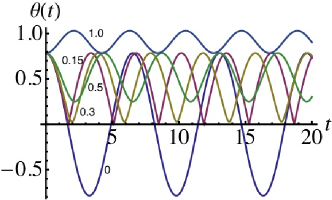
Figure 1: (Color online) $\theta(t)$ versus time for several values of the ratio of parameters $Ed/I$ and $\omega^{2}$ equal to 0, 0.15, 0.3, 0.5, and 1.

II.1 Stochastic Electric Field

Suppose that, in addition to the deterministic electric field, there is a stochastic electric field contribution, ${\bf E}=\varepsilon_{x}(t)\hat{\bf x}+\varepsilon_{y}(t)\hat{\bf y}+[E+\varepsilon_{z}(t)]\hat{\bf z}$, where $\varepsilon_{i}(t)$, $i=x,y,z$, are stochastic random variables. In what follows we explicitly take Gaussian white noise; see Eqs. (17) and (18). Other kinds of noise can occur, e.g., Gaussian colored noise or telegraph noise, but this paradigm serves to illuminate the salient features of the dynamics. Moreover, as long as the correlation time of the noise is the shortest time scale in the dynamics, Gaussian white noise is a good approximation for other kinds of noise.

If only $E_{z}$ fluctuates, we have to solve the stochastic differential equation,

$$\ddot{\theta}+\frac{d[E+\varepsilon_{z}(t)]}{I}\sin\theta-\frac{\omega^{2}}{2}\sin 2\theta=0.$$ (5)

This equation is linear in $\varepsilon_{z}(t)$, but nonlinear in $\theta$. The stochastic field $\varepsilon_{z}(t)$ results in a stochastic variation of the period of the pendular motion in $\theta$. The addition of stochastic field components $\varepsilon_{x}(t)$ and $\varepsilon_{y}(t)$ result in an additional torque which has a component along the $z$-axis, i.e., $L_{z}$ is no longer conserved, and there is an additional stochastic potential, $V_{\perp}=-({\bf d}\cdot{\bf E}_{\perp})=-p[\varepsilon_{x}(t)\sin\theta\cos\phi+\varepsilon_{y}(t)\sin\theta\sin\phi]$. Adding this potential to the potential $V=-{\bf d}\cdot{\bf E}$, we find $\frac{\partial{\cal L}}{\partial\phi}=d[-\varepsilon_{x}(t)\sin\theta\sin\phi+\varepsilon_{y}(t)\sin\theta\cos\phi]$, hence

$$\sin^{2}\theta\,\ddot{\phi}+2\sin\theta\cos\theta\,\dot{\theta}\,\dot{\phi}=\frac{d}{I}[-\varepsilon_{x}(t)\sin\theta\sin\phi+\varepsilon_{y}(t)\sin\theta\cos\phi].$$ (6)

The second order differential equations (5) and (6) can be turned into a set of first order differential equations. Defining $\vartheta(t)\equiv\dot{\theta}(t)$, Eq. (5) becomes,

$$\frac{d}{dt}\left(\!\begin{array}[]{c}\theta(t)\\ \vartheta(t)\end{array}\!\right)=\left(\begin{array}[]{c}\vartheta(t)\\ -\frac{d[E+\varepsilon_{z}(t)]}{I}\sin\theta+\frac{\omega^{2}}{2}\sin 2\theta\end{array}\right),$$ (7)

and, defining $\varphi(t)\equiv\dot{\phi}(t)$, Eq. (6) is transformed into the first order set of equations,

$$\frac{d}{dt}\left(\!\begin{array}[]{c}\phi(t)\\ \varphi(t)\end{array}\!\right)=\left(\begin{array}[]{c}\varphi(t)\\ -2\frac{\sin\theta\cos\theta}{\sin^{2}\theta}\,\dot{\vartheta}\,\dot{\varphi}+\frac{d}{I\sin^{2}\theta}[-\varepsilon_{x}(t)\sin\theta\sin\phi+\varepsilon_{y}(t)\sin\theta\cos\phi]\end{array}\right).$$ (8)

Equation (7) can be solved first for $\theta(t)$ and $\vartheta(t)$, and these functions can the be substituted into Eq. (8), which can then be used to obtain $\phi(t)$ and $\varphi(t)$. Alternatively, Eqs. (7) and (8) can be solved simultaneously as a system of four first-order differential equations.

III Quantum Treatment

The Hamiltonian for the system is given by $H=\frac{{\hat{L}}^{2}}{2I}-{\bf d}\cdot{\bf E}$ sym_top . In spherical coordinates, if the electric field is taken to be along the $z$-axis, the Hamiltonian takes the form,

$$H=-\hbar^{2}\left(\frac{\partial^{2}}{\partial\theta^{2}}+\cot\theta\frac{\partial}{\partial\theta}+\frac{1}{\sin^{2}\theta}\frac{\partial^{2}}{\partial\phi^{2}}\right)-Ed\,\cos\theta.$$ (9)

Since ${\hat{L}}_{z}$ is conserved if the electric field is along the $z$-axis, the eigenfunctions of the Hamiltonian (9) can be written as $\psi_{nm}(\theta,\phi)=e^{im\phi}f_{nm}(\theta)$, where the functions $f_{nm}(\theta)$ satisfy the stationary Schrödinger equation in one variable,

$$\left[-\frac{\hbar^{2}}{2I}\left(\frac{\partial^{2}}{\partial\theta^{2}}+\cot\theta\frac{\partial}{\partial\theta}+\frac{m^{2}}{\sin^{2}\theta}\right)+Ed\,\cos\theta\right]f_{nm}(\theta)={\cal E}_{nm}f_{nm}(\theta).$$ (10)

The energy eigenvalues ${\cal E}_{nm}$ have quadratic and higher contributions in the electric field strength.

If a degeneracy of the energy levels having different angular momentum is present, as occurs for molecules with $\Pi$ or higher electronic symmetry, a Stark energy which is linear in the electric field strength can arise. We shall not consider the dynamics for such cases here.

If, in addition to the constant electric field, a time-dependent field ${\bm{\varepsilon}}(t)=\varepsilon_{x}(t)\hat{\bf x}+\varepsilon_{y}(t)\hat{\bf y}+\varepsilon_{z}(t)\hat{\bf z}$ is present, the time-dependent Schrödinger equation must be used. A basis of states could be used to calculate the time-dependent wave function that is the solution to the time-dependent Schrödinger equation. The basis could be composed of field-free basis states $Y_{lm}(\theta,\phi)$, or the eigenstates in the presence of the constant electric field, $\psi_{nm}(\theta,\phi)$. Let us now consider the quantum treatment of the dynamics. The approach we use below uses instead the Heisenberg equations of motion, which will be solved in a mean-field approximation.

III.1 Heisenberg Equations of Motion

When no internal angular momentum is present sym_top , we take the Hamiltonian to be

$$H=H_{0}+H_{S}=\frac{{\hat{L}}^{2}}{2I}-\hat{{\bf d}}\cdot{\bf E}.$$ (11)

and we use the notation, $\hat{{\bf d}}=d\,\hat{{\bf n}}$ (see Ref. LL_QM ), where $\hat{{\bf n}}$ is a vector operator of unit length in the direction of the dipole moment and $d$ is the magnitude of the dipole moment, which remains constant. The Heisenberg equations of motion for the dipole moment operator, $\dot{\hat{{\bf d}}}=\frac{i}{\hbar}[H,\hat{{\bf d}}]$, can be written as

$$\dot{\hat{{\bf n}}}=\frac{i}{\hbar}[H,\hat{{\bf n}}]=\frac{i}{2\hbar I}[{\hat{L}}^{2},\hat{{\bf n}}]-\frac{i\,d}{\hbar}{\bf E}\cdot[\hat{{\bf n}},\hat{{\bf n}}].$$ (12)

Using the fact that $[\hat{L}_{i},\hat{n}_{j}]=i\hbar\epsilon_{ijk}\hat{n}_{k}$, we find that $[{\hat{L}}^{2},\hat{{\bf n}}]=2i\hbar[\hat{{\bf L}}\times\hat{{\bf n}}+i\hbar\,\hat{{\bf n}}]$. Since $[\hat{n}_{i},\hat{n}_{j}]=0$ for all $i$ and $j$, we find,

$$\dot{\hat{{\bf n}}}=-\frac{1}{I}[\hat{{\bf L}}\times\hat{{\bf n}}+i\hbar\,\hat{{\bf n}}].$$ (13)

Moreover, the torque on the molecule due to the presence of the external field is, $\dot{\hat{{\bf L}}}=\frac{i}{\hbar}[H,\hat{{\bf L}}]$, which reduces to

$$\dot{\hat{{\bf L}}}=-d({\bf E}\times\hat{{\bf n}}).$$ (14)

The nonlinear Heisenberg operator equations of motion, Eqs. (13) and (14), must be solved simultaneously.

III.2 Mean-Field Dynamics

If the initial angular momentum of the molecule is large compared to $\hbar$, a semiclassical treatment can be a good approximation. Setting $\hbar=0$ in Eq. (13) allows a semiclassical solution for the expectation values $\langle{\hat{{\bf n}}}(t)\rangle$ and $\langle{\hat{{\bf L}}}(t)\rangle$. The semiclassical equations,

$$\frac{d}{dt}\langle{\hat{{\bf n}}}\rangle=-\frac{1}{I}\,\langle{\hat{{\bf L}}}\rangle\times\langle{\hat{{\bf n}}}\rangle,$$ (15)

$$\frac{d}{dt}\langle{\hat{{\bf L}}}\rangle=-d\,{\bf E}\times\langle{\hat{{\bf n}}}\rangle.$$ (16)

are equivalent to the classical solution presented in Sec. II, but are valid for arbitrary direction of ${\bf E}$. These equations correspond to a mean-field theory treatment obtained by taking the expectation values of Eqs. (13) and (14), replacing the expectation value of the product $\hat{{\bf L}}\times\hat{{\bf n}}$ by the product of the expectation values Zobay_00 ; Liu_02 ; Tikhonenkov_06 ; Band_07 and taking the limit as $\hbar\to 0$ on the RHS of (13).

In what follows, we shall simplify the notation and not explicitly write the expectation values around the dynamical variables.

IV Calculated Results

We now present results for the semiclassical dynamics of a dipole moment in the presence of an electric field, with and without a stochastic contribution.

Figures 2 and 3 show $n_{x}(t),n_{y}(t)$, and $n_{z}(t)$ versus time, and Fig. 4 shows $L_{x}(t),L_{y}(t)$, and $L_{z}(t)$ versus time for deterministic dynamics (without a stochastic contribution) of a dipole moment in an electric field. The dimensionless parameters used in these calculations are $d=1$, $I=10$, and $(E_{x},E_{y},E_{z})=(0,0,1)$. The initial conditions are specified in the figure captions. $n_{z}(t)$ undergoes periodic motion, but the $n_{x}(t)$ and $n_{y}(t)$ trajectories are more complicated and are not truly periodic. Nevertheless, the motion is almost periodic with period $\tau=140$ for this case. The parametric plot of ${\bf n}(t)$ in Fig. 3 shows the holes around the north and south poles. Figure 4 shows that the total angular momentum is not conserved, but $L_{z}$ remains zero throughout the dynamics. The only component of the angular momentum that is initially nonzero is $L_{x}$. The angular momentum components $L_{x}(t)$ and $L_{y}(t)$ undergo a complicated oscillatory motion as a function of time.

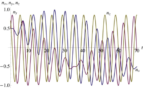
Figure 2: (Color online) $n_{x}(t),n_{y}(t)$, and $n_{z}(t)$ versus time for ${\bf n}(0)=(\sin(\pi/4)\cos(\pi/4),\sin(\pi/4)\sin(\pi/4),\cos(\pi/4))$ and ${\bf L}(0)=(10,0,0)$. The motion is almost periodic with period $\approx 140$, but only about half this region is plotted to minimize congestion.

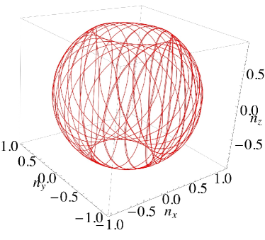
Figure 3: (Color online) Parametric plot of $n_{x}(t),n_{y}(t)$, and $n_{z}(t)$ versus time for ${\bf n}(0)=(\sin(\pi/4)\cos(\pi/4),\sin(\pi/4)\sin(\pi/4),\cos(\pi/4))$ and ${\bf L}(0)=(10,0,0)$. The motion is almost periodic (see the slight differences in the trajectory upon making two passes) with dimensionless period $\approx 140$.

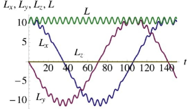
Figure 4: (Color online) $L_{x}(t),L_{y}(t),L_{z}(t)$ and $L(t)=\sqrt{L^{2}_{x}(t)+L^{2}_{y}(t)+L^{2}_{z}(t)}$ versus time for ${\bf n}(0)=(\sin(\pi/4)\cos(\pi/4),\sin(\pi/4)\sin(\pi/4),\cos(\pi/4))$ and ${\bf L}(0)=(10,0,0)$. $L_{z}(t)$ remains identically zero throughout the dynamics. The motion is almost periodic with dimensionless period $\approx 140$.

Figures 5 and 6 show $n_{x}(t),n_{y}(t)$, and $n_{z}(t)$, and Fig. 7 shows $L_{x}(t),L_{y}(t)$, and $L_{z}(t)$ versus time for deterministic dynamics for the same conditions as previously, except that now $L_{z}(0)=6$, rather than zero. Now, the $z$-component of angular momentum, which is conserved, restricts the values of $n_{z}(t)$ to be non-negative. The motion is again almost periodic, with a dimensionless period of about $\tau=100$.

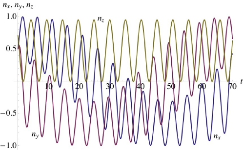
Figure 5: (Color online) $n_{x}(t),n_{y}(t)$, and $n_{z}(t)$ versus time for ${\bf n}(0)=(\sin(\pi/4)\cos(\pi/4),\sin(\pi/4)\sin(\pi/4),\cos(\pi/4))$ and ${\bf L}(0)=(10,0,6)$. The motion is almost periodic with dimensionless period $\approx 100$, but only about 70% of a period is plotted to minimize congestion.

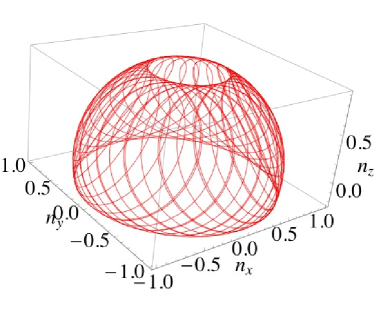
Figure 6: (Color online) Parametric plot of $n_{x}(t),n_{y}(t)$, and $n_{z}(t)$ versus time for ${\bf n}(0)=(\sin(\pi/4)\cos(\pi/4),\sin(\pi/4)\sin(\pi/4),\cos(\pi/4))$ and ${\bf L}(t)=(10,0,6)$. The motion is almost periodic (see the slight differences in the trajectory upon making two passes) with period $\approx 100$.

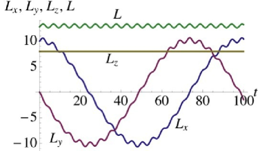
Figure 7: (Color online) $L_{x}(t),L_{y}(t),L_{z}(t)$ and $L(t)=\sqrt{L^{2}_{x}(t)+L^{2}_{y}(t)+L^{2}_{z}(t)}$ versus time for ${\bf n}(0)=(\sin(\pi/4)\cos(\pi/4),\sin(\pi/4)\sin(\pi/4),\cos(\pi/4))$ and ${\bf L}(0)=(10,0,6)$. $L_{z}(t)$ remains equal to $6$ throughout the dynamics. The motion is almost periodic with period $\approx 100$.

We now consider the details of the stochastic electric field. We take $\varepsilon_{x}(t)$ and $\varepsilon_{y}(t)$ to be stochastic processes with zero mean and correlation function $\kappa(t-t^{\prime})$ taken to be a $\delta$ function,

$$\overline{\varepsilon_{i}(t)}=0,$$ (17)

$$\overline{\varepsilon_{i}(t)\varepsilon_{j}(t^{\prime})}=\kappa(t-t^{\prime})\,\delta_{ij}=\varepsilon_{0}^{2}\,\delta(t-t^{\prime})\,\delta_{ij},$$ (18)

for $i,j=x,y$, i.e., we consider Gaussian white noise in the $x$-$y$ plane. The overline indicates the average over the fluctuations, and $\delta_{ij}$ is the Kronecker delta function (the noise in the $x$ and $y$ directions are uncorrelated). We take the correlation function $\kappa(t-t^{\prime})$ to have vanishing correlation time, $\tau_{c}=0$, i.e., Gaussian white noise. We set the strength of the fluctuations, $\varepsilon_{0}$, to be a tenth of the dc electric field $E_{z}$ with ‘volatility’ (standard deviation) $\varepsilon_{0}=0.1$, and initially take the fluctuations in the $z$-component to vanish. The equations of motion for the stochastic case are written as

$$d\langle{\hat{{\bf n}}}\rangle=-\frac{1}{I}\,\langle{\hat{{\bf L}}}\rangle\times\langle{\hat{{\bf n}}}\rangle\,dt,$$ (19)

$$d\langle{\hat{{\bf L}}}\rangle=-d\,({\bf E}\,dt+d{\bf W})\times\langle{\hat{{\bf n}}}\rangle.$$ (20)

where ${\bf W}(t)$ is a vector Wiener process. The white noise, ${\bm{\varepsilon}}(t)$ can be written as the time derivative of the Wiener process, ${\bm{\varepsilon}}(t)=d{\bf W}/dt$, or more formally, the Wiener process is the integral of the white noise. The other parameters and initial conditions are taken to be exactly as in the previous case. The stochastic field results were obtained using the Mathematica 9.0 built-in command ItoProcess for solving stochastic differential equations, with the stochastic field ${\bf W}(t)$ taken as a Wiener process. Figure 8 shows $\overline{n_{x}(t)},\overline{n_{y}(t)}$, and $\overline{n_{z}(t)}$ versus time and Fig. 9 shows $\overline{L_{x}(t)},\overline{L_{y}(t)}$, and $\overline{L_{z}(t)}$ versus time for the stochastic dynamics. In these figures, the mean values and the mean values plus and minus the standard deviations are shown, and the region between the plus and minus standard deviations are shaded. The standard deviation of $\overline{n_{x}(t)},\overline{n_{y}(t)}$, and $\overline{n_{z}(t)}$ become significant for times greater than about 70, whereas the standard deviation of $\overline{L_{x}(t)},\overline{L_{y}(t)}$, and $\overline{L_{z}(t)}$ become significant only for times greater than about 150. The mean values of $\overline{n_{x}(t)}$ and $\overline{n_{y}(t)}$ decay to zero with time, but $\overline{n_{z}(t)}$ does not decay to zero (or at least not on the time scale shown in the figure). For all $n_{i}(t)$, $i=x,y,z$, the standard deviation increases with time, but the increase is slow at large times. Moreover, the mean values $\overline{L_{x}(t)}$ and $\overline{L_{y}(t)}$ decay to zero at large time, but $\overline{L_{z}(t)}$ hardly decreases on the timescale shown, and the standard deviation of $L_{z}(t)$ increases linearly with time at large times. We conclude that, despite the fluctuations, $\overline{n_{z}(t)}$ and $\overline{L_{z}(t)}$ do not decay to zero as do the other components of $\overline{{\bf n}(t)}$ and $\overline{{\bf L}(t)}$.

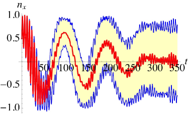
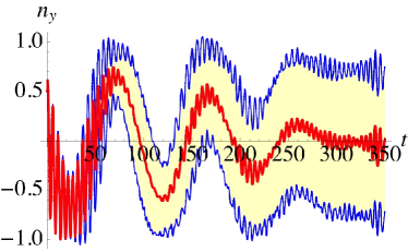
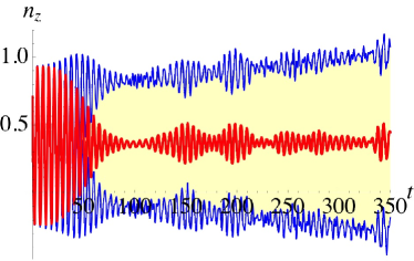
Figure 8: (Color online) $n_{x}(t),n_{y}(t),n_{z}(t)$ versus time obtained for stochastic dynamics with $\varepsilon_{x}(t)$ and $\varepsilon_{y}(t)$ fields taken as Gaussian white noise. The initial conditions are ${\bf n}(0)=(\sin(\pi/4)\cos(\pi/4),\sin(\pi/4)\sin(\pi/4),\cos(\pi/4))$ and ${\bf L}(0)=(10,0,6)$.

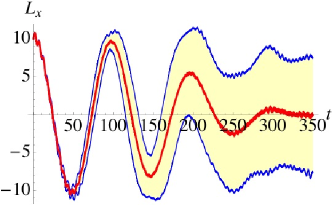
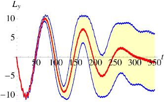
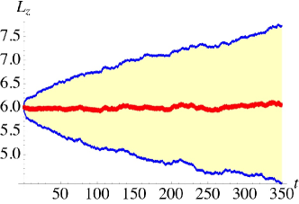
Figure 9: (Color online) $L_{x}(t),L_{y}(t),L_{z}(t)$ versus time obtained for the stochastic dynamics with $\varepsilon_{x}(t)$ and $\varepsilon_{y}(t)$ fields taken as Gaussian white noise.

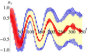
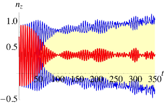
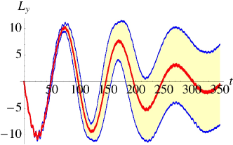
Figure 10: (Color online) Stochastic dynamics with $\varepsilon_{x}(t)$, $\varepsilon_{y}(t)$ and $\varepsilon_{z}(t)$ fields taken as Gaussian white noise. There is little change from the results shown in Figs. 8 and 9.

In Fig. 10 we also allowed the $z$-component of the electric field to fluctuate, i.e., we allowed $\varepsilon_{z}(t)$ to be a non vanishing stochastic variable with “volatility” (standard deviation) $\varepsilon_{0}=0.1$. Clearly, there is not very much of a change due to $\varepsilon_{z}(t)$. Again, despite the fluctuations of the electric field, $\overline{n_{z}(t)}$ and $\overline{L_{z}(t)}$ do not decay to zero as do the other components of $\overline{{\bf n}(t)}$ and $\overline{{\bf L}(t)}$. This is in contrast to the motion of spin in a stochastic magnetic field, where all the spin components decay to zero for Gaussian white noise in all the magnetic field components STB_2013 .

V Summary and Conclusion

We introduced a model for treating the dynamics of an electric dipole moment in the presence of a deterministic electric field and an environment with which the dipole interacts. Environmental decoherence was modeled by considering a stochastic fluctuating electric field (noise) which interacts with the electric dipole moment. We solved the stochastic mean-field equations of motion for Gaussian white noise. The model makes the external noise assumption vanKampenBook wherein no back-action of the system on the environment is present. A consequence of this assumption is that the system does not come into equilibrium with a thermal environment, but goes to the most democratic density matrix state having zero expectation value of the dipole moment STB_2013 . This is a good approximation when the back-action is weak, as explained in vanKampenBook ; STB_2013 . But even if it is not weak, one way of overcoming this problem is to augment the equations of motion for the electric dipole moment with a decay term that insures that the system comes into thermal equilibrium at long times. If we schematically represent the equation of motion for the dipole moment as, $\frac{d{\bf d}}{dt}={\cal O}{\bf d}$, and add a decay term $\eta$ to get the augmented equation of motion, $\frac{d{\bf d}}{dt}={\cal O}{\bf d}-\eta$, then at large times, we can set the rate of change of the dipole moment to be zero and the dipole moment to its equilibrium value as given by a Boltzmann averaged dipole moment, ${\bf d}_{\mathrm{eq}}={\mathrm{Tr}}[e^{-\beta H}{\bf d}]/{\mathrm{Tr}}[e^{-\beta H}]$, where $\beta$ is the inverse temperature of the bath. Hence, as $t\to\infty$, we find that $\eta={\cal O}{\bf d}_{\mathrm{eq}}$. Thus, the augmented equation of motion becomes,

$$\frac{d{\bf d}}{dt}={\cal O}(t){\bf d}(t)-{\cal O}{\bf d}_{\mathrm{eq}}.$$ (21)

This equation yields the right thermal equilibrium result asymptotically, ${\bf d}(t)\xrightarrow[t\to\infty]{}{\bf d}_{\mathrm{eq}}$. Similarly for the angular momentum equation,

$$\frac{d{\bf L}}{dt}=\tilde{\cal O}(t){\bf d}(t)-\tilde{\cal O}{\bf L}_{\mathrm{eq}},$$ (22)

where ${\bf L}_{\mathrm{eq}}={\mathrm{Tr}}[e^{-\beta H}{\bf L}]/{\mathrm{Tr}}[e^{-\beta H}]$. This approach may be overly simplistic if multiple decoherence processes play a role in the back-action dynamics, but it does yield dynamics that tend asymptotically to the correct equilibrium results when back-action is not negligible.

Here, we showed that the dynamics of an electric dipole moment in a stochastic field is more complicated than the dynamics of a magnetic dipole moment in a stochastic magnetic field. Even with the external noise assumption, and even for Gaussian white noise, not all the components of the average electric dipole moment and the average angular momentum decay to zero, despite fluctuations in all three components of the electric field. This is in contrast to the decay of the average over fluctuations of a magnetic moment, which does decay to zero in a stochastic magnetic field with Gaussian white noise in all three components STB_2013 . Here, $\overline{L_{z}(t)}\xrightarrow[t\to\infty]{}L_{z}(0)$, and $\overline{n_{z}(t)}$, which is proportional to the Stark energy, also does not decay to zero at large times; the system does not come into equilibrium. These predictions, which are valid under the external noise assumption, should be able to be readily checked experimentally. The predictions will remain valid also for Gaussian colored noise stochastic process, as long as the temporal correlation time of the noise process, $\tau_{c}$, is short compared with the rotation time of the molecule, $\tau_{r}=I/\overline{L}$, and the Stark timescale, $\tau_{S}=\hbar/(Ed)$.

- (1) P. F. Arnaiz, M. Iñarrea, J. P. Salas, Phys. Lett. A376, 1549 (2012).
- (2) B. K. Stuhl, M. T. Hummon, M. Yeo, G. Quemener, J. L. Bohn, and J. Ye, Nature 492, 396-400 (2012).
- (3) C. Scherer, Brazilian J. of Phys. 34, 442 (2004).
- (4) P. Szańkowski, M. Trippenbach and Y. B. Band, Phys. Rev. E87, 052112 (2013).
- (5) N. G. Van Kampen, Stochastic Processes in Physics and Chemistry, (Elsevier Science, 1997).
- (6) P. E. Kloeden and E. Platen, Numerical Solution of Stochastic Differential Equations, (Springer, 2011).
- (7) D. Budker, D. Kimball and D. DeMille, Atomic physics: An exploration through problems and solutions, (Oxford University Press, 2008).
- (8) S. Odenbach, Ferrofluids: Magnetically Controllable Fluids and Their Applications, (Springer, 2002); S. Odenbach, Magnetoviscous Effects in Ferrofluids, (Springer, 2002).
- (9) M. Abramowitz and I. A. Stegun, Handbook of Mathematical Functions with Formulas, Graphs, and Mathematical Tables, 9th printing, (NY, Dover) pp. 589-590, 1972.
- (10) For simplicity we take a symmetric top, rather than a spherical top or an asymmetric top Hamiltonian.
- (11) L. D. Landau and E. M. Lifshitz, Quantum Mechanics Non-relativistic Theory, Second Ed., (Pergamon Press, Oxford, 1965), pp. 312-316, and Third Ed., (Pergamon Press, Oxford, 1991) p. 337, Problem 1.
- (12) O. Zobay and B. M. Garraway, Phys. Rev. A61, 033603 (2000).
- (13) J. Liu, L. Fu, B.-Y. Ou, S.-G. Chen, D.-I. Choi, B. Wu, and Q. Niu, Phys. Rev. A66, 023404 (2002).
- (14) I. Tikhonenkov, E. Pazy, Y. B. Band, M. Fleischhauer, and A. Vardi, Phys. Rev. A 73 (2006).
- (15) Y. B. Band, I. Tikhonenkov, E. Pazyy, M. Fleischhauer, and A. Vardi, J. of Modern Optics 54, 697-706 (2007).