Phase diagram of the 4D $U(1)$ model at finite temperature.

Abstract

We explore the phase diagram of the 4D compact $U(1)$ gauge theory at finite temperature as a function of the gauge coupling and of the compactified Euclidean time dimension $L_{t}$. We show that the strong-to-weak coupling transition, which is first order at $T=0$ ($L_{t}=\infty$), becomes second order for high temperatures, i.e. for small values of $L_{t}$, with a tricritical temporal size $\bar{L}_{t}$ located between 5 and 6. The critical behavior around the tricritical point explains and reconciles previous contradictory evidences found in the literature.

I Introduction

Discerning the critical behavior taking place at a given phase transition by numerical simulations can be a very challenging problem, especially when one has to distinguish between a second order transition and a very weak first order transition.

A beautiful example is given by the Abelian compact $U(1)$ gauge theory in four dimensions in the Wilson discretization: in this formulation the theory is defined on the 4D Euclidean hypercubic space-time lattice, the fundamental dynamical variables are the parallel transports along the links $U_{\mu}(x)=\exp(ieaA_{\mu}(x))$ ($a$ is the lattice spacing) and the action is:

$$S_{W}=\beta\sum_{x,\mu>\nu}\Big{(}1-\mathrm{Re}\,\Pi_{\mu\nu}(x)\Big{)}\ ,$$ (1)

where the plaquette $\Pi_{\mu\nu}(x)$ is defined as

$$\Pi_{\mu\nu}(x)=U_{\mu}(x)U_{\nu}(x+\hat{\mu})U_{\mu}^{{\dagger}}(x+\hat{\nu})U_{\nu}^{{\dagger}}(x)\ .$$ (2)

It is well known, since the early formulation of the model, that it has two different phases: a weak coupling Coulomb phase and a strong coupling confined phase. The existence of these two phases was rigorously proved, for a different form of the action, in Ref. Guth , while for the Wilson action (1) evidence of this phase structure is based on numerical simulations (for recent results see e.g. Refs.DGP ; Jersak99 ; VdP ; MKK ; P ). The nature of the transition separating the two phases has been debated for a long time, the final conclusion being that the transition is weak first order Jersak83 ; Arnold01 ; Arnold03 . This conclusion is important since it implies that no continuum Quantum Field Theory can be defined for the $U(1)$ gauge theory at the critical point, since the correlation length stays finite.

More recently, a finite temperature version of the model has been considered, in which the Euclidean temporal size $L_{t}$ is compactified and kept fixed, while the thermodynamical limit is reached by sending to infinity the spatial sizes, $L_{s}\to\infty$. The model shows a non-trivial phase structure in the $1/L_{t}-\beta$ plane. For $L_{t}=1$, the system gets exactly decoupled into a 3D $XY$ model and a 3D $U(1)$ lattice gauge theory: the former undergoes a second order phase transition at $\beta_{c}=0.4541652(5)(6)$ (see Ref. Campostrini06 ) while the latter is known to be always in the confined phase (see Refs. Polyakov76 ; Gopfert81 ), therefore a single phase transition is expected, in the 3D XY universality class. Such phase transition extends also to $L_{t}\neq 1$ and corresponds to the spontaneous breaking of a symmetry analogous to that of the $XY$ model, i.e. a global $U(1)$ symmetry. This is generated by gauge transformations which are periodic in time only up to a given global phase, and an order parameter for this symmetry is the Wilson line taken along the Euclidean temporal direction, i.e. the Polyakov loop. For $L_{t}\to\infty$, the breaking of this symmetry corresponds to the confining-to-Coulomb transition of the 4D theory, which is known to be first order. A possible further transition line may be present, in principle, separating a weak-coupling phase with spatial confinement at small $L_{t}$ from the zero-temperature Coulomb phase, however evidence has been presented in Ref. vettorazzo that such line could be actually placed at $L_{t}\to\infty$.

A natural question is how the order of the $U(1)$-breaking transition changes as one moves from $L_{t}=1$, where it is second order, to $L_{t}=\infty$, where it is first order. Notice that, for every value of $L_{t}$, the fact that an exact global symmetry exists guarantees that a true phase transition must be found, associated with its spontaneous breaking.

This issue has been discussed for the first time in Ref. vettorazzo , where it has been proposed that the transition may stay first order at least for $L_{t}$ down to $L_{t}=6$, turning into second order for lower $L_{t}$. The evidence in that case was based on the analysis of the time histories on large lattices (up to $6\times 60^{3}$), showing clear signs of metastability. However, due to computational limitations, statistics presented in Ref. vettorazzo were not enough to reach a definite conclusion.

On the contrary, in a subsequent investigation, the authors of Ref. berg have suggested that a finite size scaling analysis gives evidence for a second order transition at $L_{t}=6$, with critical indexes similar to that of a Gaussian point (see also Ref. berg_lat ). The authors of Ref. berg find Gaussian indexes, instead of the expected XY indexes, also for smaller values of $L_{t}$, down to $L_{t}=4$. The problem in the analysis of Ref. berg , as pointed out by the authors themselves and as we will clarify later, is the limited number of available spatial sizes, going up to $L_{s}=18$, which does not permit a correct extrapolation to the thermodynamical limit.

In the present study we solve the issue, reconciling evidence from Ref. vettorazzo and berg . In particular, we will show that the transition is indeed first order down to $L_{t}=6$, turning into second order for lower values of $L_{t}$. The separation between the two different regimes is marked, as it always happens in these cases, by a tricritical point, which, even if not exactly located at an integer value of $L_{t}$, influences the scaling of nearby values of $L_{t}$. As a consequence, the correct scaling on such points, first order or second order, is not visible until large enough values of the spatial size $L_{s}$ are reached. On small lattices, instead, the true scaling behavior is obscured by a fake tricritical scaling, which has indeed the mean field tricritical (Gaussian) indexes observed in Ref. berg . This variation of the scaling behavior with the lattice size is typical of tricritical points and is observed in Monte Carlo simulations of many other models, going from QCD at finite baryon chemical potential (see e.g Refs. DES ; dFP ; BCDES ; BdFDEPS ) to the Potts model in an external magnetic field (Ref. BDE ). The simplest physical systems which exhibit tricritical behavior are probably fluid mixtures but, as should also be clear from the previous discussion, tricritical phenomena appear to be ubiquitous in physics (see e.g. Ref. LawSarb ). In relation to our study, particularly intriguing is the presence of tricritical points in superconductors (see Refs. Kleinert82 ; Kleinert06 ): Ginzburg-Landau theory of superconductivity is based on an $U(1)$ gauge theory (with matter) and the tricritical behavior is triggered by vortex line defects, which are present also in the lattice $U(1)$ gauge theory.

The paper is organized as follows. In Section II we present a general overview of the quantities and the methods adopted to probe the critical behavior around the transition; in Section III we present and discuss numerical results obtained for various values of $L_{t}$; finally, in Section IV, we draw our conclusions.

II Observables and numerical analysis setup

	$\nu$	$\gamma$	$\alpha$	$\gamma/\nu$	$\alpha/\nu$
$3D$ XY	0.6717(1)	1.3178(2)	-0.0151(3)	1.962	$-$0.0225
Tricritical	1/2	1	1/2	2	1
$1^{st}$ Order	1/3	1	1	3	3

Table 1: Critical exponents (see Campostrini06 and e.g. landau ; pelissvic ).

In lattice gauge theories, the natural observables are mean values of path ordered products of link variables. The simplest path that can be used is the boundary of an elementary square, the corresponding observable being the mean value of the plaquette operator

$$W=\frac{1}{6L_{t}L_{s}^{3}}\sum_{x}\mathrm{Re}\,\Pi_{\mu\nu}(x)\ ,$$ (3)

where $\Pi_{\mu\nu}(x)$ is defined in Eq. (2). $W$ is proportional (up to an additive constant) to the energy density of the system.

The other variable that will be used is the Polyakov loop: in this case the path is a straight line along the temporal direction, which closes because of the periodic boundary conditions in the temporal direction,

$$P=\frac{1}{L_{s}^{3}}\sum_{\mathbf{x}}\prod_{t=0}^{L_{t}-1}U_{0}(t,\mathbf{x})\ ,$$ (4)

where $\mathbf{x}$ denotes a generic point of the $t=0$ slice of the lattice. As noted in the introduction this observable is an order parameter for the breaking of a global $U(1)$ symmetry. For larger gauge groups a non-vanishing $P$ value signals the breaking of the center symmetry, which in our case is just the group itself, being $U(1)$ abelian. The fact that the transition of the ($3+1$)D $U(1)$ gauge theory, if second order, is in the universality class of the 3D $XY$ model, can be viewed as a particular realization of the Svetitsky-Yaffe conjecture (Ref. svya ).

Our goal is to show that the order of the deconfinement transition changes by increasing $L_{t}$. To this aim we need to study, at fixed $L_{t}$, the critical behavior of the system for $L_{s}\to\infty$, in order to discriminate between a first and a second order transition. We will thus study the susceptibilities of $W$ and $P$, defined by

$$C_{V}=L_{t}L_{s}^{3}\ (\langle W^{2}\rangle-\langle W\rangle^{2})$$ (5)

and

$$\chi=L_{t}L_{s}^{3}\ (\langle|P|^{2}\rangle-\langle|P|\rangle^{2})\,.$$ (6)

Near the phase transition, the scaling of these two quantities as functions of the spatial size $L_{s}$ is given (up to additive analytic contributions) by

$$C_{V} \sim L_{s}^{\alpha/\nu}\ f_{1}(tL_{s}^{1/\nu})$$ (7)

$$\chi \sim L_{s}^{\gamma/\nu}\ f_{2}(tL_{s}^{1/\nu})\ ,$$

where $t\equiv(T-T_{c})/T_{c}$ is the reduced temperature and the $f_{i}$’s are universal scaling functions, i.e. they depend only on the universality class of the (second order) transition. From these relations it follows in particular that the scaling of the height of the peaks is governed by the exponents $\alpha/\nu$ and $\gamma/\nu$ respectively. The critical indexes which will be relevant in the following are those of the 3D $XY$ model, the tricritical and the first order ones. Their numerical values are reported for convenience in Table 1.

Figure 1: Plot of the regions where the different critical behaviors are expected to be seen on finite volumes. The sector where tricritical scaling dominates shrinks to zero in the thermodynamic limit but can be very large for small volumes.

It was noted in Ref. BDE that it is increasingly difficult to correctly identify the order of the transition as we approach a tricritical point, since larger and larger volumes are needed in order to disentangle the true thermodynamic behavior from a fictitious tricritical scaling for small volumes (see Fig. 1 for a pictorial representation). In fact it can be shown BDE ; pelissvic ; BinderDeutsch that the spatial lattice size required for an unambiguous identification of the transition scales as

$$L_{s}\sim A|L_{t}-\bar{L}_{t}|^{-1}$$ (8)

where $A$ is a constant and $\bar{L}_{t}$ is the tricritical point value.

It thus follows that, in order to locate with precision the tricritical point, we cannot simply look for regions of the parameter space where a tricritical scaling is observed. A better strategy is to study observables which quantify the strength of the first order transition, like the discontinuities at the transition, and analyze their variation as a function of the external parameter ($L_{t}$ in our case) in order to extrapolate the point where they vanish, which is just the tricritical point.

We will denote by $\Delta_{W}$ and $\Delta_{P}$, respectively, the discontinuities across the (possible) first order transition of the mean plaquette and of the Polyakov loop. These quantities can be estimated by looking at the scaling of the maxima of the relative susceptibilities at the transition: if the volume is large enough (i.e. if $L_{s}$ is much larger than the correlation length) we have

$$(C_{V})_{max}\sim L_{t}L_{s}^{3}\,\Delta_{W}^{2}$$ (9)

$$(\chi)_{max}\sim L_{t}L_{s}^{3}\,\Delta_{P}^{2}\ .$$

Another estimator for $\Delta_{W}$ is the Binder-Challa-Landau cumulant Challa , which is defined by

$$B_{4}=1-\frac{\langle W^{4}\rangle}{3\langle W^{2}\rangle^{2}}\ .$$ (10)

It can indeed be shown (see e.g. Ref. LeeKosterlitz ) that near a transition $B_{4}$ develops a minimum, whose depth scales like

$$B_{4}|_{min}\simeq\frac{2}{3}-\frac{1}{3}\left(\frac{\Delta_{W}}{\epsilon}\right)^{2}$$ (11)

where $\epsilon=\frac{1}{2}(W^{+}+W^{-})$ and $W^{\pm}=\lim_{\beta\to\beta_{c}^{\pm}}\langle W\rangle$. In particular, the thermodynamical limit of $B|_{min}$ is strictly less than $2/3$ if and only if a discontinuity is present. In order to simplify the notation in the following we will adopt the shorthand $B=\frac{2}{3}-B_{4}|_{min}$.

The discontinuities $\Delta_{W}$ and $\Delta_{P}$ decrease as we approach the tricritical temporal size $\bar{L}_{t}$ from the first order side (i.e. from $L_{t}>\bar{L}_{t}$) and the leading order behavior is (see Ref. LawSarb or Sheehy for a brief summary of the main results)

$$\Delta_{W}\propto\sqrt{L_{t}-\bar{L}_{t}}$$ (12)

and

$$\Delta_{P}\propto\sqrt{|(L_{t}-\bar{L}_{t})\log(L_{t}-\bar{L}_{t})|}\ .$$ (13)

In systems for which the tricritical behavior is triggered by a continuous variable (like e.g. the one studied in Ref. BDE ) it is typically possible to approach the tricritical point close enough to observe a scaling of the form in Eqs. (12)-(13). In the case at study, the relevant variable is discrete and it is not possible to observe such a scaling behavior. A different strategy could be to study the 4D $U(1)$ gauge theory with an asymmetric coupling in the temporal direction, which effectively reduces the temporal size in a continuous way. However, in the present investigation we will limit ourselves to the isotropic case already studied in Refs. vettorazzo and berg .

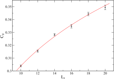
Figure 2: Values of the $C_{V}$ maxima for $L_{t}=2$. The line is a fit with a function of the form $a+bL_{s}^{\alpha/\nu}$, where for $\alpha$ and $\nu$ the 3D $XY$ values are used ($\chi^{2}/\mathrm{d.o.f.}\approx 1.2$).

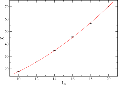
Figure 3: Values of the $\chi$ maxima for $L_{t}=2$. The line is a fit with a function of the form $a+bL_{s}^{\gamma/\nu}$, where for $\gamma$ and $\nu$ the 3D $XY$ values are used ($\chi^{2}/\mathrm{d.o.f.}\approx 1.1$).

III Numerical Results

Since we are going to study the region of first order transitions near the tricritical point, the strength of the discontinuities will never be large enough to justify the use of algorithms specifically designed for strong first orders, like e.g. the multicanonical algorithm BergNeuhaus . For this reason, we adopt a mixture of heatbath Moriarty and overrelaxation Creutz updates in the ratio $1:5$. Data have been analyzed by means of standard jackknife and multi-histogram reweighing algorithms (see e.g. Refs. BergMCMC ; NewmanBarkema and FS1 ; FS2 ). In all the cases $\mathcal{O}(10)$ $\beta$ values were simulated, and for each one $\mathcal{O}(10^{3})$ independent measures have been performed (which amounts to $\mathcal{O}(10^{6}\div 10^{7})$ elementary update sweeps).

Our first aim is to show that for small $L_{t}$ the transition is second order in the 3D $XY$ universality class. In order to prove that, we studied the system with the smallest nontrivial value of $L_{t}$, namely $L_{t}=2$. In Figs. 2 and 3 the maxima of $C_{V}$ and $\chi$, respectively, are plotted for increasing $L_{s}$ values, and a nice agreement with the theoretical expectations based on the 3D $XY$ exponents is observed.

However, the right question to ask is to what extent we can distinguish the critical behavior dictated by the 3D $XY$ indexes from that corresponding to tricritical indexes (coinciding with Gaussian indexes), so as to exclude the latter. We do not learn much from the scaling of $\chi$ in Fig. 3: if we leave the critical exponent as a free parameter we get $\gamma/\nu=1.939(45)$, which is compatible with both behaviors (see Table 1).

Instead, if we look at the plaquette susceptibility, Fig. 2, we learn that on small lattices (i.e. $L_{s}\lesssim 14$) the behavior is still compatible with Gaussian indexes ($\alpha/\nu=1$), while on larger lattices deviations are significant, indicating the need for $\alpha/\nu<1$; the 3D $XY$ exponent, on the contrary, describes well all the explored range of $L_{s}$.

The outcome for $L_{t}=2$ is therefore that on small lattices the transition can be (erroneously) associated with Gaussian critical exponents, while on large enough lattices the transition is clearly described by the 3D $XY$ indices, with no significant contaminations from tricritical scaling.

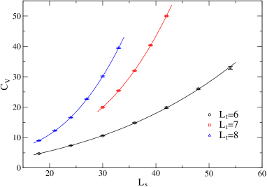
Figure 4: Values of the $C_{V}$ maxima for $L_{t}=6,7,8$. The lines are fits with a function of the form (14), with $\lambda_{t}=1$ ($\chi^{2}/\mathrm{d.o.f.}\approx 0.5,1.1,0.7$ for $L_{t}=6,7,8$ respectively).

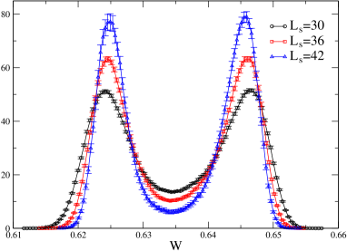
Figure 5: Histograms of the plaquette distribution at transition for $L_{t}=7$ and three different spatial extent.

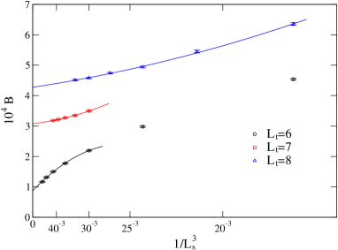
Figure 6: Values of $B=2/3-B_{4}|_{min}$ for $L_{t}=6,7,8$. The lines are fits with $a+bx+cx^{2}$ ($\chi^{2}/\mathrm{d.o.f.}\approx 1.0,0.2,0.7$ for $L_{t}=6,7,8$ respectively).

The situation is different for $L_{t}=6$ or larger, where the transition turns out to be first order, however we had to study lattices up to $L_{s}=54$ to clearly determine the true critical behavior. Even on the larger lattices, indeed, the tricritical contribution, although no more dominant, is nevertheless significant. To correctly describe the maxima of the susceptibilities we had to use a function of the form

$$f_{\chi}(L_{s})=a+bL_{t}L_{s}^{\lambda_{t}}+cL_{t}L_{s}^{3}$$ (14)

where $L_{s}^{3}$ is the behavior expected at a first order transition, while the sub-leading term $L_{s}^{\lambda_{t}}$ is a correction with the exponent of the tricritical case ($\lambda_{t}=1$ and $2$ for the plaquette and Polyakov loop respectively). The $L_{t}$ multiplicative terms follow from the normalization of the susceptibilities in Eqs. (5)-(6). Even for the plaquette susceptibility, for which $\lambda_{t}=1$, the sub-leading term is in fact the larger one for $L_{s}$ up to $\approx 45$, and contributes $\approx 88\%$ of the total singular part for $L_{s}=18$ (which was the largest spatial size explored in Ref. berg ).

The agreement between the data and the fits of the form (14) is good, as shown in Fig. 4 for the susceptibility of the plaquette and for $L_{t}=6,7,8$. From Fig. 4 it can be noticed that the first order transition gets stronger with increasing $L_{t}$, as theoretically expected. In Fig. 5 we show the nice double peak structure which develops in the plaquette distribution at the transition temperature, which gets more and more pronounced as the thermodynamical limit is approached.

A consistent picture emerges from the study of the Binder cumulant: in Fig. 6 the values of $B=2/3-B_{4}|_{min}$ are shown for $L_{t}=6,7,8$ together with parabolic fits. The reason for the parabolic fits is that finite size corrections to $B$ are known to be analytic in $1/V$ for first order transitions, see Ref. LeeKosterlitz . Remembering Eq. (11), it is evident from Fig. 6 that the first order transition gets stronger as $L_{t}$ increases.

Following the strategy outlined in Section II, we will now determine the parameters which fix the strength of the first order transition, in order to extrapolate the critical value $\bar{L}_{t}$ at which the first order disappears. The parameters are the latent heat, or equivalently the minimum of the Challa-Landau-Binder cumulant defined in Eq. (11), and the gap of the order parameter.

$L_{t}$	$\Delta_{W}^{2}$	$\Delta_{P}^{2}$	$B$
$6$	$2.04(5)\times 10^{-5}$	$1.5(3)\times 10^{-3}$	$8.7(3)\times 10^{-5}$
$7$	$1.06(6)\times 10^{-4}$	$4.98(8)\times 10^{-3}$	$3.08(2)\times 10^{-4}$
$8$	$1.39(3)\times 10^{-4}$	$3.64(7)\times 10^{-3}$	$4.27(4)\times 10^{-4}$

Table 2: Estimated values for the parameters $\Delta_{W}$, $\Delta_{P}$ (defined by Eq. (LABEL:suscmax)), and $B=2/3-B_{4}|_{min}$ (see Eq. (11)).

The latent heat and the gap of the order parameter can be extracted from the large volume limit of the maxima of the susceptibilities, see Eq. (LABEL:suscmax). Since we have seen that the tricritical component significantly contributes to the susceptibilities also for large volumes, we decided to adopt the coefficient $c$ in Eq. (14) as an estimator of the gap, in order to clearly disentangle the first order contribution from the tricritical one.

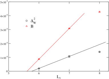
Figure 7: Estimates of the endpoint: the lines are linear interpolations of the $L_{t}=6,7$ data (see text).

The values of $\Delta_{W}^{2}$ and $\Delta_{P}^{2}$ estimated from the fits are reported in Table 2. The behavior of $\Delta_{W}$ is qualitatively consistent with the theoretical expectations on the first order getting stronger with increasing $L_{t}$, while $\Delta_{P}$ is non-monotonic with respect to $L_{t}$. This can be explained by noting that, while the plaquette is a local observable, the Polyakov loop is an extended object directly related to $L_{t}$. As a consequence, the gap in the Polyakov loop at the transition cannot in general be directly connected to the strength of the transition; on the contrary, we expect that the gap vanishes in the limit $L_{t}\to\infty$, since in such limit the Polyakov loop tends to zero also in the deconfined phase. It is nevertheless surprising that the results obtained for just three $L_{t}$ values (and in fact for the three smallest values for which a first order transition is present, see later) are sufficient to expose this non-monotonic behavior.

By fitting the Binder cumulant values we can estimate the value of $B$ in the thermodynamical limit (see again Table 2 for the results). This is just $\Delta_{W}^{2}$ multiplied by a function of $L_{t}$ which is expected not to vanish nor to have singularities at the tricritical point (see Eq. (11)). The behavior of $B$ near the tricritical point should thus be the same as that of $\Delta_{W}^{2}$.

The expected scaling of $\Delta_{W}$ in the neighbourhood of the tricritical point is given by Eq. (12), i.e. $\Delta_{W}^{2}$ (and thus also $B$) should depend linearly on $L_{t}$. However, as previously noted, we cannot expect to be able to really observe this scaling, since $L_{t}$ assumes only discrete values and thus we are not allowed to approach the tricritical point with arbitrary precision.

As can be seen in Fig. 7, strong deviations from the leading linear behavior are indeed clearly visible even on the data for three consecutive $L_{t}$ values. However the discrete nature of $L_{t}$, which introduces such complication, also gives us the possibility to avoid a precise determination of the tricritical value $\bar{L}_{t}$: we only need to determine the two consecutive integers such that $\bar{L}_{t}$ is located in between, such task may be unfeasible only in the unlucky situation in which $\bar{L}_{t}$ itself is very close to an integer.

$B$ and $\Delta_{W}^{2}$ in Fig. 7 appear to be concave functions of $L_{t}$, hence we can obtain an underestimate for $\bar{L}_{t}$ by imposing the vanishing of the linear interpolation obtained from the two lowest values of $L_{t}$, i.e. $L_{t}=6$ and 7. As can be seen from Fig. 12, this underestimate is significantly larger than $L_{t}=5$. On the other hand, we know that for $L_{t}=6$ the transition is first order. Therefore, we can safely conclude that $5<\bar{L}_{t}<6$.

A direct check of this statement could be obtained by studying the $L_{t}=5$ system and verifying the presence of a second order transition in the 3D $XY$ universality class. Such a direct check seems however to be more difficult than the corresponding one performed on the first order side for $L_{t}=6$. Indeed, the critical exponents of the 3D $XY$ class are smaller than the tricritical ones (the opposite happens instead for first order exponents), so that a direct identification of the universality class to which the $L_{t}=5$ transition belongs, might be much harder.

IV Conclusions

In the present study we have investigated the 4D compact $U(1)$ gauge theory at finite temperature, i.e. on lattices with a finite Euclidean temporal dimension $L_{t}$, compactified with periodic boundary conditions. In particular, we have determined the order of the strong-to-weak coupling transition as a function of $L_{t}$.

The transition is first order for $L_{t}\geq 6$ and second order, in the universality class of the 3D $XY$ model, for $L_{t}\leq 5$. A tricritical point is thus present at a non-integer value $\bar{L}_{t}$, with $5<\bar{L}_{t}<6$. The tricritical scaling associated with this point influences, for nearby values of $L_{t}$, the scaling of relevant susceptibilities in a range intermediate spatial sizes $L_{s}$, thus explaining and reconciling the contradictory evidence reported in previous literature vettorazzo ; berg .

Evidence for the presence of a first order transition has been direct on all explored lattices, $L_{t}=6,7,8$. Evidence for a second order transition has been direct for $L_{t}=2$ and indirect for $L_{t}=3,4,5$, in particular based on the vanishing of the first order gap for lattices with $L_{t}\leq 5$.

An accurate verification of the correct scaling around the tricritical point has not been possible, due to the discrete nature of the temporal extension $L_{t}$. That could be done in a different setup, namely working on anisotropic lattices, with two different couplings for spatial and temporal plaquettes, and approaching the tricritical point by tuning the temporal gauge coupling. We leave that to future studies.

Finally, let us remark, following the conclusions of Ref. vettorazzo , that speaking of finite temperature, in the case of the compactified 4D $U(1)$ gauge theory that we have studied, is not completely appropriate, in particular in connection with the continuum limit of the theory. Indeed, the $a\to 0$ limit is possible only in correspondence of second order transition points, but since these are limited to values of $L_{t}\leq 5$, a true continuum limit at fixed physical temperature $T=1/(L_{t}a)$ is not possible. This is at variance with ordinary non-Abelian gauge theories at finite temperature, where instead one can send at same time $L_{t}\to\infty$ and $a\to 0$, keeping a fixed physical value of $T$.

Appendix A Numerical data

In this appendix we report the numerical data used in the analysis. The pseudo-critical coupling $\beta_{pc}$ is defined by the position of the peak in the Polyakov loop susceptibility.

$L_{s}$	max $C_{V}$	min $B_{4}$	max $\chi$	$\beta_{pc}$
10	0.30392(73)	0.6658711(18)	17.786(53)	0.8956(12)
12	0.31546(85)	0.6661848(13)	25.563(87)	0.89720(97)
14	0.32821(88)	0.66635101(89)	34.73(12)	0.89827(83)
16	0.3347(13)	0.66644968(86)	45.64(24)	0.89901(71)
18	0.3443(13)	0.66651002(61)	56.71(29)	0.89938(66)
20	0.3494(17)	0.66654987(56)	70.10(42)	0.89985(62)

Table 3: Values for $L_{t}=2$.

$L_{s}$	max $C_{V}$	min $B_{4}$	max $\chi$	$\beta_{pc}$
18	4.733(29)	0.6662128(28)	139.59(89)	1.009329(48)
24	7.370(52)	0.6663686(22)	270.4(1.8)	1.009474(23)
30	10.606(82)	0.6664471(17)	461.7(3.1)	1.009542(14)
36	14.82(11)	0.6664891(14)	733.3(5.2)	1.0095727(93)
42	19.87(22)	0.6665167(17)	1089(11)	1.0095877(76)
48	26.02(27)	0.6665350(13)	1560(15)	1.0095976(49)
54	32.92(46)	0.6665498(16)	2119(27)	1.0096083(45)

Table 4: Values for $L_{t}=6$.

$L_{s}$	max $C_{V}$	min $B_{4}$	max $\chi$	$\beta_{pc}$
30	19.98(11)	0.6663168(19)	566.1(2.8)	1.0102814(72)
33	25.45(12)	0.6663319(15)	755.8(3.3)	1.0102910(49)
36	31.98(12)	0.6663395(11)	998.3(3.3)	1.0103034(34)
39	40.40(12)	0.6663449(10)	1297.0(3.6)	1.0103134(25)
42	50.00(14)	0.66634863(97)	1655.2(4.5)	1.0103190(21)

Table 5: Values for $L_{t}=7$.

$L_{s}$	max $C_{V}$	min $B_{4}$	max $\chi$	$\beta_{pc}$
18	8.989(68)	0.6660313(45)	125.86(74)	1.010453(24)
21	12.28(10)	0.6661217(46)	188.0(1.3)	1.010528(19)
24	16.599(92)	0.6661728(27)	274.8(1.2)	1.0105830(97)
27	22.70(12)	0.6661929(25)	397.1(1.9)	1.0106238(71)
30	30.12(15)	0.6662085(23)	553.4(2.4)	1.0106372(48)
33	39.50(19)	0.6662155(21)	750.2(3.1)	1.0106464(39)

Table 6: Values for $L_{t}=8$.

References

- (1) A. H. Guth Phys. Rev. D 21, 2291 (1980).
- (2) A. Di Giacomo, G. Paffuti Phys. Rev. D 56, 6816 (1997) [hep-lat/9707003].
- (3) J. Jersak, T. Neuhaus, H. Pfeiffer Phys.Rev. D 60, 054502 (1999) [hep-lat/9903034].
- (4) M. Vettorazzo, P de Forcrand Nucl. Phys. B 686, 85 (2004) [hep-lat/0311006]
- (5) P. Majumdar, Y. Koma, M. Koma Nucl. Phys. B 677, 273 (2004) [hep-lat/0309003].
- (6) M. Panero JHEP 0505, 066 (2005) [hep-lat/0503024].
- (7) J. Jersak, T. Neuhaus, P. Zerwas, Phys. Lett. B 133 (1983) 103.
- (8) G. Arnold, T. Lippert, T. Neuhaus, K. Schilling, Nucl. Phys. B (Proc. Suppl.) 94, 651 (2001) [hep-lat/0011058].
- (9) G. Arnold, B. Bunk, T. Lippert, K. Schilling, Nucl. Phys. B (Proc. Suppl.) 119, 864 (2003) [hep-lat/0210010].
- (10) M. Campostrini, M. Hasenbusch, A. Pelissetto, E. Vicari Phys.Rev. B 74, 144506 (2006) [cond-mat/0605083].
- (11) A. M. Polyakov, Nucl. Phys. B 120, 429 (1977).
- (12) M. Gopfert, G. Mack, Commun. Math. Phys. 82, 545 (1982).
- (13) M. Vettorazzo, P. de Forcrand, Phys. Lett. B 604, 82 (2004) [hep-lat/0409135].
- (14) B. A. Berg, A. Bazavov, Phys. Rev. D 74, 094502 (2006) [hep-lat/0605019].
- (15) B. A. Berg, A. Bazavov PoS LAT2006:061 (2006) [hep-lat/0609006].
- (16) M. D’Elia, F. Sanfilippo, Phys. Rev. D 80, 111501 (2009) [0909.0254].
- (17) P. de Forcrand, O. Philipsen, Phys. Rev. Lett. 105, 152001 (2010) [1004.3144].
- (18) C. Bonati, G. Cossu, M. D’Elia, F. Sanfilippo, Phys. Rev. D 83, 054505 (2011) [1011.4515].
- (19) C. Bonati, P. de Forcrand, M. D’Elia, O. Philipsen, F. Sanfilippo, PoS LATTICE 2011, 189 (2011) [arXiv:1201.2769 [hep-lat]].
- (20) C. Bonati, M D’Elia, Phys. Rev. D 82, 114515 (2010) [1010.3639].
- (21) I. D. Lawrie, S. Sarbach, Theory of Tricritical Points, in C. Domb, J. L. Lebowitz (eds.) “Phase transitions and critical phenomena, vol. 9”, Academic Press (1987).
- (22) H. Kleinert Lett. Nuovo Cimento 35, 405 (1982).
- (23) H. Kleinert Europhys. Lett 74, 889 (2006).
- (24) B. Svetitsky and L.G. Yaffe, Nucl. Phys. B 210, 423 (1982).
- (25) L. D. Landau, E. M. Lifshitz, “Statistical Physics, Part 1”, Butterworth Heinemann (1980).
- (26) A. Pelissetto, E. Vicari, Phys. Rep. 368, 549 (2002) [cond-mat/0012164].
- (27) K. Binder, H. P. Deutsch, Europhys. Lett. 18, 667 (1992).
- (28) M. S. S. Challa, D. P. Landau, K. Binder, Phys. Rev. B 34, 1841 (1986).
- (29) J. Lee, J. M. Kosterlitz, Phys. Rev. B 43, 3265 (1991).
- (30) D. E. Sheehy, Phys. Rev. A 79, 033606 (2009) [0807.0922].
- (31) B. A. Berg, T. Neuhaus Phys. Rev. Lett. 68, 9 (1992) [hep-lat/9202004].
- (32) K. J. M. Moriarty, Phys. Rev. D 25 2185 (1982).
- (33) M. Creutz, Phys. Rev. D 36, 515 (1987).
- (34) B. A. Berg “Markov Chain Monte Carlo Simulations and Their Statistical Analysis”, World Scientific (2004).
- (35) M. E. J. Newman, G. T. Barkema “Monte Carlo Methods in Statistical Physics”, Clarendon Press (2001).
- (36) A. M. Ferrenberg, R. H. Swendsen, Phys. Rev. Lett. 61, 2635 (1988).
- (37) A. M. Ferrenberg, R. H. Swendsen, Phys. Rev. Lett. 63, 1195 (1989).