Competing orders in the 2D half-filled SU($2N$) Hubbard model through the pinning field quantum Monte-Carlo simulations

Abstract

We non-perturbatively investigate the ground state magnetic properties of the 2D half-filled SU($2N$) Hubbard model in the square lattice by using the projector determinant quantum Monte Carlo simulations combined with the method of local pinning fields. Long-range Neel orders are found for both the SU(4) and SU(6) cases at small and intermediate values of $U$. In both cases, the long-range Neel moments exhibit non-monotonic behavior with respect to $U$, which first grow and then drop as $U$ increases. This result is fundamentally different from the SU(2) case in which the Neel moments increase monotonically and saturate. In the SU(6) case, a transition to the columnar dimer phase is found in the strong interaction regime.

The ultra-cold atom systems have opened up a wonderful opportunity for studying novel phenomena which are not easily accessible in usual solid state systems. For example, the large-spin ultra-cold alkali and alkaline-earth fermions exhibit quantum magnetic properties fundamentally different from the large-spin solid state systems such as transition metal oxides Wu (2012). In solids, Hund’s rule coupling combines several electrons on the same cation site into states carrying large spin $S$. However, the symmetry of these systems is usually only SU(2). The leading order coupling between two neighboring sites is mediated by exchanging one pair of electrons no matter how large $S$ is, thus quantum spin fluctuations are suppressed by the $1/S$-effect. In contrast, large-hyperfine-spin ultra-cold fermion systems can possess high symmetries of SU($2N$) and Sp($2N$). For the simplest case of spin-$\frac{3}{2}$, a generic Sp(4) symmetry was proved without fine-tuning, which includes the SU(4) symmetry as a special case Wu et al. (2003); *Wu2006. Such a high symmetry gives rise to exotic properties in quantum magnetism and pairing superfluidity Wu (2005); Hattori (2005); Lecheminant et al. (2005); Controzzi and Tsvelik (2006); Cazalilla et al. (2009); Wu et al. (2010); Rodríguez et al. (2010); Corboz et al. (2011); Hung et al. (2011); Szirmai and Lewenstein (2011). Furthermore, large-spin alkaline-earth fermion systems have been experimentally realized in recent years DeSalvo et al. (2010); Taie et al. (2010); Krauser et al. (2012). In particular, an SU(6) Mott insulator of ¹⁷³Yb has also been observed Taie et al. (2012); Wu (2012). The above theoretical and experimental progress has stimulated a great deal of interests in exploring novel properties of strongly correlated systems with high symmetries Hermele et al. (2009); Gorshkov et al. (2010); Cai et al. (2013a); Messio and Mila (2012); Cai et al. (2013b); Szirmai et al. (2011); Sinkovicz et al. (2013).

The SU($2N$) Heisenberg model was first introduced into condensed matter physics to apply the large-$N$ technique to systematically handle strong correlation effects in the context of high $T_{c}$ cuprates Affleck (1985); Arovas and Auerbach (1988); Affleck and Marston (1988); Read and Sachdev (1989, 1989). It was found that on 2D bipartite lattices the SU(2) Heisenberg model displays long-range Neel ordering Anderson (1952). As $2N$ increases, enhanced quantum fluctuations suppress Neel ordering and the ground states eventually become dimerized Read and Sachdev (1989, 1989). This transition has been observed by quantum Monte Carlo (QMC) simulations Harada et al. (2003); Kawashima and Tanabe (2007); Beach et al. (2009); Kaul and Sandvik (2012); Paramekanti and Marston (2007); Assaad (2005) for certain representations of the SU($2N$)symmetry . However, for the self-conjugate representations, a consensus has not been achieved yet. A variational Monte Carlo study Paramekanti and Marston (2007) found Neel ordering when $2N=2$ and $4$, and columnar dimer ordering for $2N\geq 6$. However, in a determinant QMC calculation Assaad (2005), dimer ordering was found at $2N\geq 6$ in agreement with the variational QMC study, while for the SU(4) case, neither Neel nor dimer ordering exists in the Heisenberg limit.

The above Heisenberg-type models neglect charge fluctuations. The interplay between charge and spin degrees of freedom is contained in the SU($2N$) Hubbard model Lu (1994); Honerkamp and Hofstetter (2004); Cai et al. (2013b). However, owing to the lack of non-perturbative methods, the SU($2N$) Hubbard model receives much less attention. To the best of our knowledge, a systematic non-perturbative study of the ground state properties of the 2D half-filled models is still missing. It is even not clear whether Neel or dimer ordering exists in the weak, intermediate and strong coupling regimes, respectively.

In this article, we perform a non-perturbative determinant QMC study on the half-filled SU($2N$) Hubbard model in the 2D square lattice. The ground state magnetic properties are investigated by using the local pinning field method which directly measures the spatial decay of the induced order parameters White and Chernyshev (2007). Long-range Neel order is identified at weak and intermediate values of $U$ in the SU($2N$) Hubbard models of $2\leq 2N\leq 6$ we studied. In the cases of SU(4) and SU(6), the Neel moments first grow then drop with increasing $U$. Furthermore, a transition from the Neel-ordering phase into the columnar dimer-ordering phase is observed at a large value of $U$ in the SU(6) case. This transition is conceivably owing to the competition between the weak coupling physics of Fermi surface nesting and strong coupling local moment physics.

We consider the SU($2N$) Hubbard model in the 2D square lattice with the periodic boundary condition as,

$$H=-t\sum_{\langle i,j\rangle,\alpha}\left(c_{i\alpha}^{\dagger}c_{j\alpha}+h.c.\right)+\frac{U}{2}\sum_{i}\left(n_{i}-N\right)^{2},$$ (1)

where $t$ is the nearest neighbor hopping integral ($t=1$ in the below); $U$ is the on-site repulsion; $\alpha$ is the spin index running from $1$ to $2N$; $n_{i}=\sum_{\alpha=1}^{2N}n_{i\alpha}$is the total fermion number operator on site $i$. Eq. 1 possesses the particle-hole symmetry $c_{i\alpha}\rightarrow(-)^{i}c_{i\alpha}^{\dagger}$, which means that it is at half-filling. In this case, it is well-known that Eq. 1 is free of the sign problem for all the values of $N$.

We employ the projector QMC to investigate its quantum magnetic properties in the ground states. In QMC studies, the long-range ordering is usually obtained through the finite-size scaling of the corresponding structural factors, or, correlation functions. Assuming that the system size is $L\times L$, the extrapolated values as $L\rightarrow\infty$ are proportional to the magnitude square of order parameters. Thus it is difficult to distinguish the weakly ordered states from the truly disordered ones. For this reason, there has been a debate whether a quantum spin liquid phase exists near the Mott transition in the honeycomb lattice Meng et al. (2010); Li (2011); Sorella et al. (2012); Hassan and Sénéchal (2013); Assaad and Herbut (2013); *Assaad2012. To overcome this difficulty, we use the pinning field method White and Chernyshev (2007); Assaad and Herbut (2013); *Assaad2012, and measure the spatial decay of the induced order parameters. Order parameters instead of their magnitude square are measured, and thus numerically they are more sensitive to weak orderings. This method has also been used in the projector QMC recently Assaad and Herbut (2013). To decouple the interaction term, we adopt the Hubbard-Stratonovich (HS) transformation in the density channel which involves complex numbers Hirsch (1983). We have designed a new discrete HS decomposition which is exact for the cases from SU(2) to SU(6) Hubbard models, and the algorithm details can be found in the Supplementary Material. Unless specifically stated, the following parameters are used in simulations: the projection time $\beta=240$ and the discretized imaginary time step $\Delta\tau=0.05$.

Next we use the pinning field method to study the magnetic long-range order of the SU($2N$) Hubbard model. We define the SU($2N$) generators as $S^{\alpha\beta}_{i}=c^{\dagger}_{i,\alpha}c_{i,\beta}-\frac{\delta^{\alpha\beta}}{2N}n_{i}$. At half-filling, in the Heisenberg limit in which charge fluctuations are neglected, each site belongs to the self-conjugate representation with one column of $N$ boxes. Without loss of generality, the classic Neel state configuration can be chosen as follows: each site in sublattice $A$ is filled with $N$ fermions from components $1$ to $N$, while that in sublattice $B$ is filled with components from $N+1$ to $2N$. We define the magnetic moment operator on each site $i$ as

$$m_{i}=\frac{1}{2N}\big{\{}\sum_{\alpha=1}^{N}S^{\alpha\alpha}_{i}-\sum_{\alpha=N+1}^{2N}S^{\alpha\alpha}_{i}\big{\}}.$$ (2)

For the configuration defined above, the value of the classic Neel moment is $m_{i}=(-)^{i}\frac{1}{2}$. Within the zero temperature projector QMC method, good quantum numbers are conserved during the projection. Thus we use a pair of pinning fields on two neighboring sites with a Neel configuration to maintain the relation $\langle G|\sum_{i}S^{\alpha\alpha}_{i}|G\rangle=0$ for every $\alpha$. The pinning field Hamiltonian is

$$H_{pin,n}=2Nh_{i_{0}j_{0}}\big{\{}m_{i_{0}}-m_{j_{0}}\big{\}},$$ (3)

where $i_{0}$ and $j_{0}$ are two neighboring sites defined as $i_{0}=(1,1)$ and $j_{0}=(2,1)$, respectively. The initial trial wavefunctions can be chosen as the half-filled plane-wave states. The Hamiltonian Eq. 1 plus Eq. 3 remains free of the sign problem at half-filling.

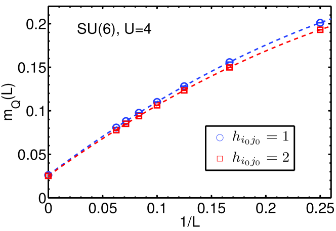
Figure 1: Finite size scaling of the residual Neel moment $m_{Q}(L)$ v.s. $1/L$ under pinning fields described by Eq. 3 with $h_{i_{0}j_{0}}=1$ and $2$. The largest value of $L$ is 16. The quadratic polynomial fitting is used. Error bars are smaller than symbols.

Because the pinning fields in Eq. 2 break the $SU(2N)$ symmetry, the induced magnetic moments prefer the direction defined in Eq. 2. The distribution of $m_{i}$ is staggered with decaying magnitudes as away from two pinned sites $i_{0}$ and $j_{0}$. The Neel order parameter is its Fourier component at the wavevector $Q=(\pi,\pi)$ defined as $m_{Q}(L)=\frac{1}{L^{2}}\sum_{i}(-)^{i}m_{i}$. The long-range order $m_{Q}$ can be extrapolated as the limit of

$$m_{Q}=\lim_{L\rightarrow\infty}m_{Q}(L).$$ (4)

This is because the Fourier component of the pinning field at $Q$ is $h_{Q}=2h_{i_{0}j_{0}}/L^{2}$, which goes to zero as $L\rightarrow\infty$ for any finite value of $h_{i_{0}j_{0}}$.

To illustrate the sensitivity of the pinning field method to weak orders, we present the simulations for the SU(6) case of Eq. 1 with $U=4$. The finite size scalings of $m_{Q}(L)$ are presented in Fig. 1 for two different values of $h_{i_{0}j_{0}}=1$ and $2$. Their extrapolated values as $1/L\rightarrow 0$ are $0.0261\pm 0.0008$ and $0.0253\pm 0.0009$, respectively, which are consistent with each other and confirm the validity of this method. Such a small moment is hard to identify using the finite size scaling of the structural factors, as shown in the Supplementary Material and related worksMeng et al. (2010); Sorella et al. (2012); Assaad and Herbut (2013); *Assaad2012. Another observation is that the induced values of $m_{Q}(L)$ are weaker at $h_{i_{0}j_{0}}=2$ than those at $h_{i_{0}j_{0}}=1$ at finite values of $L$, which shows non-linear correlations between the pinning centers and the measured sites. Certainly they converge in the limit of $1/L\rightarrow 0$. In the following, we only present the results of $h_{i_{0}j_{0}}=2$.

One may question whether the pinning field method overestimates the tendency of long-range ordering. In the Supplementary Material, we apply it to the 1D SU(2) and SU(4) Hubbard chains at half-filling. In the SU(2) case, the ground state is known as a gapless spin liquid, while in the SU(4) case, it is gapped with dimerization. The pinning field method shows the absence of long-range Neel ordering in both cases and the asymptotic behavior of power-law spin correlations in the case of SU(2). This further confirms the validity of this method.

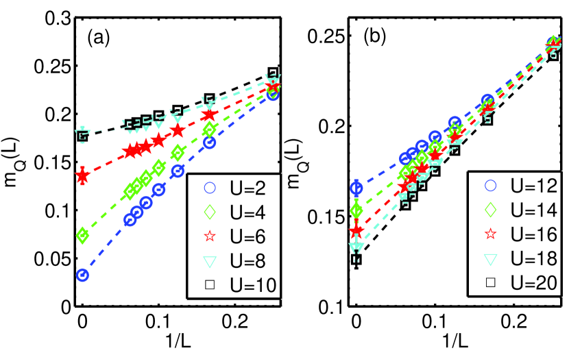
Figure 2: Finite size scalings of $m_{Q}(L)$ v.s. $1/L$ for the half-filled SU(4) Hubbard model with different values of $U$. The largest size is $L=16$. The quadratic polynomial fitting is used. Error bars of QMC data are smaller than symbols.

We further test the validity of the pinning field method in the extensively studied half-filled SU(2) Hubbard model in the square lattice by QMC Hirsch (1985); Varney et al. (2009). The long-range Neel ordering we obtained based on the pinning field method is consistent with that in previous QMC literature based on the finite-size scaling of structure factors. Our results are shown in the Supplementary material. The long-range Neel ordering appears from weak to strong interactions. The extrapolated values of $m_{Q}$ increase as $U$ goes up, and begin to saturate around $U=10$. At $U=20$, $m_{Q}=0.297\pm 0.002$, which is in a good agreement with the long-range Neel moment $0.3070(3)$ of the SU(2) Heisenberg model Sandvik (1997). This behavior is well-known Hirsch (1985); Varney et al. (2009): as $U$ goes up, charge fluctuations are suppressed, and thus the low energy physics is described by the Heisenberg model.

Next we simulate the SU(4) Hubbard model and the magnetic ordering is presented in Fig. 2. Similarly to the SU(2) case, long-range Neel ordering appears for all the values of $U\leq 20$. At each value of $U$, the extrapolated long-range Neel moment $m_{Q}$ is weaker than that in the SU(2) case, which is a result of the enhanced quantum fluctuations. Moreover, a striking new feature appears that the relation $m_{Q}$ v.s. $U$ becomes non-monotonic as shown in Fig. 4 below. The Neel moment $m_{Q}$ reaches the maximum around $0.178\pm 0.008$ at $U\approx 8$, and then decreases as $U$ further increases. It remains finite with the largest value of $U=20$ in our simulations. It is not clear whether $m_{Q}$ is suppressed to zero or not in the limit of $U\rightarrow\infty$. A previous QMC simulation on the SU(4) Heisenberg model shows algebraic spin correlations Assaad (2005). It would be interesting to further investigate whether the algebraic spin liquid state survives at finite values of $U$.

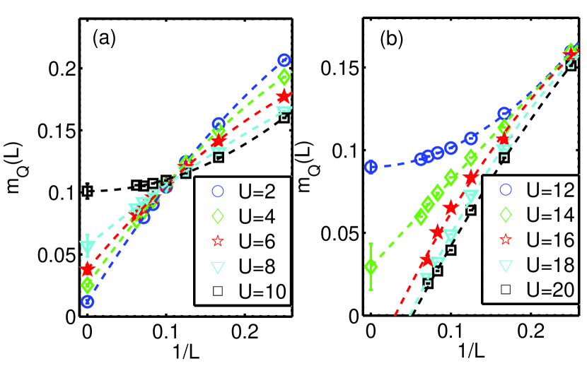
Figure 3: Finite size scalings of $m_{Q}(L)$ v.s. $1/L$ for the SU(6) Hubbard model at different values of $U$. The largest size is $L=16$. The quadratic polynomial fitting is used. Error bars of QMC data are smaller than symbols.

With further increases in $2N$, the Neel ordering is more strongly suppressed by quantum spin fluctuations. The finite-size scalings for the SU(6) case at different values of $U$ are presented in Fig. 3. For all the values of $U\leq 14$, we find nonzero Neel ordering by using the quadratic polynomial fitting. The extrapolated Neel moment $m_{Q}$ v.s. $U$ for the SU(6) case are plotted in Fig. 4. For comparison, those of the SU(2) and SU(4) are also plotted together. Similar to the SU(4) case, the long-range Neel moments are non-monotonic which reach the maximum around $U\approx 10$. Strikingly, the Neel ordering disappears beyond a critical value of $U_{c}$ which is estimated as $14<U_{c}<16$.

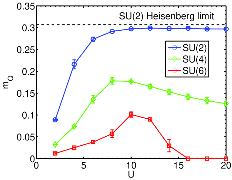
Figure 4: The ground state Neel ordering of the 2D half-filled SU($2N$) Hubbard model in the square lattice. The relations of long-range Neel moments $m_{Q}$ v.s. $U$ are plotted for $2N=2,4$ and $6$. For comparison, the SU(2) Heisenberg limit result is plotted as the dotted line. The error bars are obtained from the least square fittings with $95\%$ confidence bounds.

The low energy effective model of half-filled Hubbard models in the strong coupling regime is the Heisenberg model. According to the large-$N$ study of the SU($2N$) Heisenberg model with the self-conjugate $1^{N}$ representation Read and Sachdev (1989, 1989), dimerization appears in the large-$N$ limit. Thus the suppression of the Neel order at large values of $U$ is expected from the competing dimer ordering. To investigate this competition, we further apply the pinning field method to study the dimer ordering for the SU(6) Hubbard model and results are presented in Fig. 5. The following dimer pinning field is applied, which changes the hopping integral of a bond $i_{0}j_{0}$ ,

$$H_{pin,dim}=-\Delta t_{i_{0}j_{0}}\sum_{\alpha}\Big{\{}c_{i_{0},\alpha}^{\dagger}c_{j_{0},\alpha}+h.c.\Big{\}},$$ (5)

where $i_{0}$ and $j_{0}$ are defined before. The bonding strength between sites $i$ and $i+\hat{x}$ is defined as $d_{i,x}=\frac{1}{2}\langle G|c_{i\alpha}^{\dagger}c_{i+x,\alpha}+h.c.|G\rangle$, where $|G\rangle$ is the ground state. We define the dimer order parameter at the wavevector $(\pi,0)$ as

$$\mbox{dim}_{(\pi,0)}(L)=\frac{1}{L^{2}}\sum_{i}(-)^{i_{x}}d_{i,x},$$ (6)

where $i_{x}$ is the $x$-coordinate of site $i$. Following the same reasoning to extrapolate the long-range Neel ordering before, we define the long-range dimer order parameter as $\mbox{dim}_{(\pi,0)}=\lim_{L\rightarrow\infty}\mbox{dim}_{Q}(L)$. The finite size scalings for $\mbox{dim}_{(\pi,0)}(L)$ are plotted in Fig. 5 (a), which shows the columnar dimerization appears when $U$ is above a critical value $U_{c}^{\prime}$ which is also estimated around $14\sim 16$. It lies in the same interaction regime that Neel ordering starts to vanish. However, whether this transition is of second order such that $U_{c}=U_{c}^{\prime}$, or, it is of first order, still needs further numeric investigation. We also measure the dimerization at $Q=(\pi,\pi)$ induced by the pinning field Eq. 5, defined as $\mbox{dim}_{(\pi,\pi)}(L)=\frac{1}{L^{2}}\sum_{i}(-)^{i}d_{i,x}$, whose finite size scaling shows the absence of long-range order.

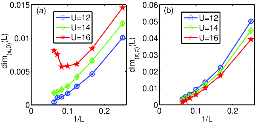
Figure 5: Finite size scalings of the dimer order parameters in the half-filled SU(6) Hubbard model. (a) $\mbox{dim}_{(\pi,0)}(L)$ and (b) $\mbox{dim}_{(\pi,\pi)}(L)$ at wavevectors $Q^{\prime}=(\pi,0)$ and $Q=(\pi,\pi)$, respectively. The largest size is $L=16$. Error bars of QMC data are smaller than symbols.

The nature of the transition between the Neel and dimer orderings is an interesting question. In the literature Senthil et al. (2004); Sandvik (2007), ring exchange terms are added to the SU(2) Heisenberg model, which suppress Neel ordering and lead to dimerization. However, our SU(6) case is dramatically different. The SU(6) Neel ordering appears in the regime of weak and intermediate interactions. In this regime ring exchanges are prominent because they reflect short-range charge fluctuations. Our results agree with the picture of Fermi surface nesting because the Neel ordering wavevector $Q=(\pi,\pi)$ is commensurate with the Fermi surface at half-filling, while dimerization is not favored because its wavevector $Q^{\prime}=(\pi,0)$ does not satisfy the nesting condition . On the other hand, local moment physics dominates when deeply inside the Mott insulating phase in the strong coupling regime. The exchange energy per site in the dimerized phase is estimated at the order of $N^{2}J$ with $J=4t^{2}/U$, while that of the Neel state is $zNJ$ where $z$ is the coordination number. Thus dimerization wins when both conditions of large-$U$ and large-$N$ limits are met in agreement with previous theoretical results on SU($2N$) Heisenberg models Read and Sachdev (1989).

Summary.— We have applied the method of local pinning fields in QMC simulations to investigate quantum magnetic properties of the 2D half-filled SU($2N$) Hubbard model in the square lattice. This method is sensitive to weak long-range orders. Long-range Neel ordering is found for the SU(4) case from weak to strong interactions. For the SU(6) case, a transition from the staggered Neel ordering to the columnar dimerization is found with increasing $U$. The conceivable mechanism is the competition between the weak coupling Fermi surface nesting physics and the strong coupling local moment physics. The above QMC simulations may provide a reference point for further investigating the even more challenging problem of doped SU($2N$) Mott-insulators.

Acknowledgment.— We thank J. E. Hirsch, Y. Wan for helpful discussions. Especially, we thank H. H. Hung for providing numeric results from exact diagonalizations for comparison. D. W., Y. L., and C. W. are supported by the NSF DMR-1105945 and AFOSR FA9550-11-1- 0067(YIP); Z. C. thanks the German Research Foundation through DFG FOR 801. Z. Z., Y. W. and C. W. acknowledge the financial support from the National Natural Science Foundation of China (11328403, J1210061), and the Fundamental Research Funds for the Central Universities. Y. L. thanks the Inamori Fellowship and the support at the Princeton Center for Theoretical Science. We acknowledge support from the Center for Scientific Computing from the CNSI, MRL: an NSF MRSEC (DMR-1121053) and NSF CNS-0960316.

Supplementary Material

In this supplementary material, we explain the algorithm of the projector quantum Monte Carlo method in Sect. A. Various tests of the local pinning field method are presented in Sect. B. The error analysis is performed in Sect. C.

Appendix A Projector quantum Monte Carlo and Hubbard-Stratonovich decomposition

We adopt the projector determinant QMC method Assaad and Evertz (2008) to study the half-filled SU($2N$) Hubbard model. The basic idea is to apply the projection operator $\mathrm{e}^{-\beta H/2}$ on a trial wave function $|\Psi_{T}\rangle$. If $\langle\Psi_{G}|\Psi_{T}\rangle\neq 0$ and there exists a nonzero gap between $|\Psi_{G}\rangle$ and the first excited state, $|\Psi_{G}\rangle$ is arrived as the projection time $\beta\rightarrow\infty$,

$$|\Psi_{G}\rangle=\lim_{\beta\rightarrow\infty}\mathrm{e}^{-\beta H/2}|\Psi_{T}\rangle.$$ (7)

The projection time $\beta$ can be divided into $M$ slices with $\beta=M\Delta\tau$.

The second order Suzuki-Trotter decomposition is used to separate the kinetic and interaction energy parts in each time slice,

$$\mathrm{e}^{-\Delta\tau(K+V)}=\mathrm{e}^{-\Delta\tau K/2}\mathrm{e}^{-\Delta\tau V}\mathrm{e}^{-\Delta\tau K/2}+o[(\Delta\tau)^{3}],$$ (8)

where $K$ and $V$ represent the kinetic and interaction terms, respectively. For the $V$ term, a discrete Hubbard-Stratonovich (HS) transformation is defined as Hirsch (1983)

$$e^{-\lambda^{2}(n_{i}-N)^{2}}=\frac{1}{4}\sum_{\mathclap{l=\pm 1,\pm 2}}\gamma_{i}(l)e^{i\eta_{i}(l)(n_{i}-N)}+o[(\Delta\tau)^{4}],$$ (9)

where $n_{i}=\sum_{\alpha=1}^{2N}c^{\dagger}_{i\alpha}c_{i\alpha}$; $\lambda=\sqrt{\Delta\tau U/2}$; $\gamma$’s and $\eta$’s are discrete HS fields given by the following values Assaad

$$\gamma(\pm 1) = 1+\frac{\sqrt{6}}{3},\ \ \,\ \ \,\gamma(\pm 2)=1-\frac{\sqrt{6}}{3},$$

$$\eta(\pm 1) = \pm\sqrt{\Delta\tau U}\sqrt{3-\sqrt{6}},$$

$$\eta(\pm 2) = \pm\sqrt{\Delta\tau U}\sqrt{3+\sqrt{6}}.$$ (10)

This decomposition is widely used in QMC simulations Wu and Zhang (2005); Assaad . However, one should be careful that at large values of $U$ and $|n-N|$ in Eq. 9. In Fig. 6, we plot the values of the left and right hand sides of Eq. 9 as functions of $\Delta\tau U$ for comparison. We consider the situations of $|n-N|=1,2$ and $3$, respectively. The errors of this discrete HS decomposition Eq. 10 depend on $|n-N|$ significantly. At $|n-N|=1$ and $2$, the decomposition yields values almost exact, or, with slight deviations for $\Delta\tau U<1$. However, at $|n-N|=3$, the deviation becomes manifest when $\Delta\tau U>0.5$, and even more terribly, the weight becomes negative.

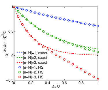
Figure 6: Error due to the HS decomposition using parameters defined in Eq. 10. The dashed lines are exact results of $\mathrm{e}^{-\Delta\tau U(n_{i}-N)^{2}/2}$ with $|n-N|=1,2,3$ respectively. The circles represent the results after the HS transformation.

Therefore, we design an exact HS decomposition for the cases from SU(2) to SU(6) in which the operator $n_{i}-N$ only takes eigenvalues among $0,\pm 1,\pm 2$, and $\pm 3$. The form of the new HS decomposition is the same as Eq. 10 but it is exact. The values of the discrete HS fields are defined as follows

$$\gamma(\pm 1) = \frac{-a(3+a^{2})+d}{d},\ \ \,\ \ \,\gamma(\pm 2)=\frac{a(3+a^{2})+d}{d},$$

$$\eta(\pm 1) = \pm\cos^{-1}\left\{\frac{a+2a^{3}+a^{5}+(a^{2}-1)d}{4}\right\}$$

$$\eta(\pm 2) = \pm\cos^{-1}\left\{\frac{a+2a^{3}+a^{5}-(a^{2}-1)d}{4}\right\},$$ (11)

where $a=e^{-\frac{1}{2}\Delta\tau U}$, $d=\sqrt{8+a^{2}(3+a^{2})^{2}}$. Eq. 11 is used for all of our simulations in 2D SU($2N$) Hubbard model in the main text.

After integrating out fermions, we arrive at the fermion determinant whose value depends on the discrete HS fields. The HS fields are sampled using the standard Monte Carlo technique.

Appendix B Tests of the pinning field method

Below we present various tests of the pinning field method to confirm its validity and its sensitivity to weak orderings.

B.1 Test of the pinning field method in the half-filled SU(2) Hubbard model

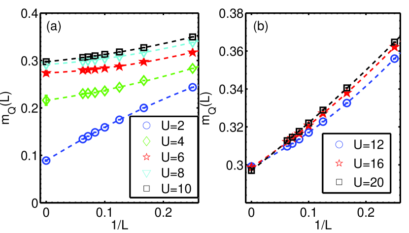
Figure 7: Finite size scalings of $m_{Q}(L)$ v.s. $1/L$ for the half-filled SU(2) Hubbard model. The lines are fitted by the quadratic polynomial fitting of the QMC data. Error bars of QMC data are smaller than symbols.

We have performed the QMC simulations with the local pinning field method for the half-filled SU(2) Hubbard model in the square lattice. The finite-size scaling is presented in Fig. 7. The parameter values are the pinning field $h_{i_{0}j_{0}}=2$ and the projection time $\beta=240$. The extrapolated values of the Neel moments $m_{Q}$ defined in Eq. increase monotonically as $U$ increases and become to saturate around $U=10$. The Neel moment reaches $0.297\pm 0.002$ at $U=20$ in our simulation, which agrees well with previous QMC simulations. This test confirms the validity of the pinning field method.

B.2 Sensitivity of the pinning field method to weak ordering

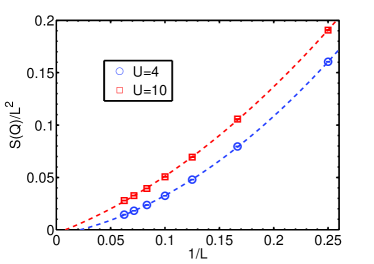
Figure 8: Finite size scalings of the structure factor $S(Q)/L^{2}$ in the case of SU(6) with $U=4$ and $U=10$. Quadratic polynomials are used to fit the data. Error bars of QMC data are smaller than symbols. In these calculations, projection time $\beta=80$ is used.

We consider the cases of weak Neel ordering in the half-filled SU(6) Hubbard model in the square lattice with $U=4$ and $U=10$. The finite-size scalings based on structure factor are shown in Fig. 8. Quadratic polynomials are used to fit the structure factor $S(Q)/L^{2}$ as defined in Ref.  Cai et al., 2013b. It is difficult to conclude whether long-range Neel ordering exists or not in both cases. In contrast, for the case of $U=4$, the finite-size scaling based on the pinning field method in Fig. 1 in the main text yields the extrapolated Neel moment $m_{Q}=0.026$. The corresponding value of $S(Q)/L^{2}$ is its square at the order of $10^{-3}$ and thus is too weak to identify in Fig. 8. Moreover, for the case of $U=10$ in which the largest Neel moment appears (Fig. 4 in the main text), the corresponding structure factor remains too small to be extrapolated through the finite size scaling. The weak Neel orderings in the SU(6) Hubbard model were not found in a previous work based on the structure factor method by some of the authors either Cai et al. (2013b). Due to the improved numeric resolution, they are identified through the pinning field method.

B.3 The pinning field method for the 1D SU(2) and SU(4) Hubbard models

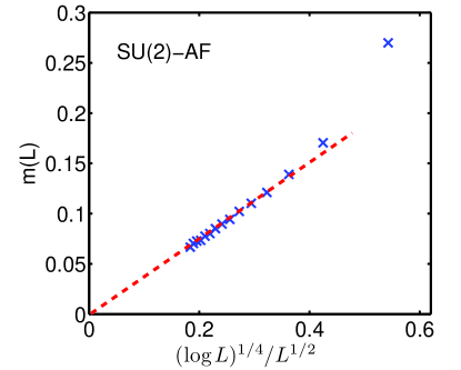
Figure 9: Finite size scaling of $m(L)$ v.s. $(\log L)^{\frac{1}{4}}/L^{\frac{1}{2}}$ for the 1D half-filled SU(2) Hubbard model. Parameter values are $\beta=80$, $U=4$ and $h_{i_{0}j_{0}}=2$.

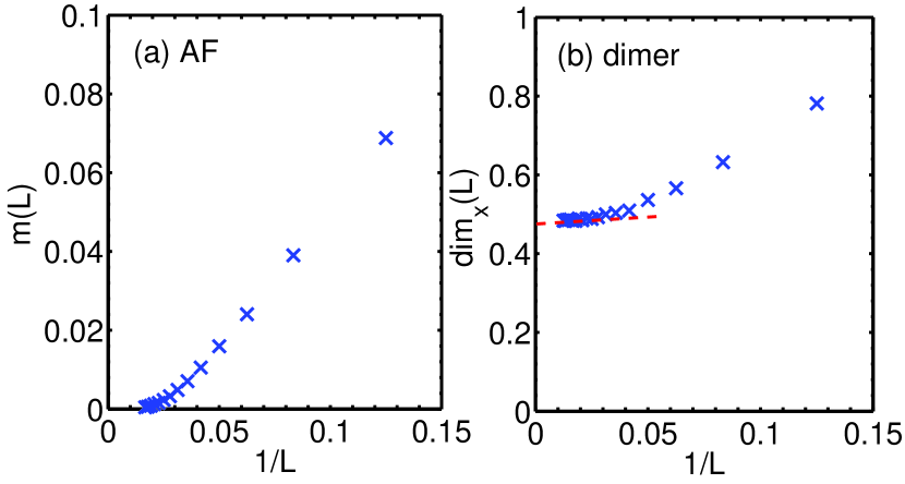
Figure 10: (a) Finite size scaling of $m(L)$ v.s. $1/L$ for the 1D half-filled SU(4) Hubbard model. (b) Finite size scaling of $\mbox{dim}_{x}(L)$ v.s. $1/L$ for the 1D half-filled SU(4) Hubbard model. Parameter values are $\beta=80$, $U=4$ and $\Delta t_{i_{0}j_{0}}=2$.

Since the pinning field method is sensitive to weak long-range orderings, a natural question is that whether it is oversensitive. To clarify this issue, we apply it to 1D half-filled SU(2) and SU(4) Hubbard models in which it is well-known that magnetic long-range orders do not exist. The QMC simulation results presented below are in an excellent agreement with previous analytic and numeric results. This confirms the validity of the pinning field method. We use the pinning fields described in the Eq. 3 and Eq. 5 in the main text to investigate Neel and dimer orderings, respectively.

For the 1D half-filled SU(2) Hubbard model, the pinned sites are set as $i_{0}=1$ and $j_{0}=2$, respectively, and values of the pinning fields are $h_{i_{0},j_{0}}=2$. We consider the induced magnetic moment on the furthest sites $\frac{L}{2}$ and $\frac{L}{2}+1$ defined as $\pm m(L)$. Strong quantum fluctuations suppress the long-range Neel ordering, and the asymptotic behavior of the two-point spin correlation functions at half-filling follows the pow-law decay as Schulz (1990)

$$\langle S(i)S(j)\rangle\sim(-)^{i-j}\frac{\log^{\frac{1}{2}}|i-j|}{|i-j|}.$$ (12)

Since spin moments are pinned at $i_{0}$ and $j_{0}$, $m(L)$ should scales as

$$m(L)\sim\frac{(\log L)^{\frac{1}{4}}}{\sqrt{L}}.$$ (13)

Our QMC results with pinning fields are in an excellent agreement with Eq. 12 as shown in Fig. 9.

The magnetic properties of the 1D half-filled SU(4) Hubbard model are dramatically different from the SU(2) case. Bosonization analysis Wu (2005) shows that its ground states exhibit long-range-ordered dimerization with a finite spin gap, and the Neel correlation decays exponentially. We set the pinned sites at $i_{0}=1$ and $j_{0}=2$, respectively, and the pinning field for dimerization as $\Delta t_{i_{0}j_{0}}=2$. The induced dimer order is defined as the difference between two furthest bonds $(\frac{L}{2},\frac{L}{2}+1)$ and $(\frac{L}{2}+1,\frac{L}{2}+2)$ as

$$\mbox{dim}_{i}(L)=(-)^{i}\big{\{}d_{L/2,x}-d_{L/2+1,x}\big{\}}.$$ (14)

Our QMC simulation results are illustrated in Fig. 10 (b), which exhibit the long-range ordering in agreement with previous analytic results.

B.4 The issue of non-linear response to the pinning field

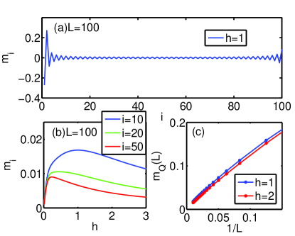
Figure 11: The induced magnetic moments $m(i)$ by pinning fields in the non-interacting half-filled 1D SU(2) lattice model. (a) The spacial distribution of $m(i)$ with $h_{i_{0}j_{0}}=1$ and $L=100$. (b) The induced moments $m(i)$ v.s $h_{i_{0},j_{0}}$ at different sites $i=10,20$ and $50$ in the system with $L=100$. (c) The scaling of $m_{Q}(L)$ with $Q=\pi$ at two different pinning fields.

In Fig. 1 of the main text, we present the scaling of the residual Neel moment $m_{Q}(L)$ $v.s.$ $1/L$ with two different values of the pinning fields. A counter-intuitive observation is that $m(L)$ is weaker at $h_{i_{0}j_{0}}=2$ than that of $h_{i_{0}j_{0}}=1$. Below we present convincing evidence that actually this is not an artifact of the finite size. This is a typical behavior of responses on sites far away from the scattering center in the strong scattering limit.

To illustrate this point, we present the calculation for a toy model of a non-interacting half-filled SU(2) 1D lattice system, such that we can easily calculate systems with very large size up to $L=100$. The pinning fields are located at sites $i_{0}=1$ and $j_{0}=2$, and the induced magnetic moments $m(i)$ are presented in Fig. 11. Although it is natural that the induced magnetic moments increase monotonically with $h$ right on the impurity sites, there is no reason to expect the same behavior on sites away from the scattering center. On these sites, in fact, Fig. 11(b) shows that $m(i)$’s are non-monotonic with respect to $h$. All of them decays at large values of $h$ after passing maxima at intermediate values of $h$. The finite size scalings of $m_{Q}(L)$ defined in the main text are presented in Fig. 11(c) at $h=1$ and 2. Both curves converge to 0 as they should be in non-interacting systems. Again, the curve with $h=2$ is lower than that of $h=1$.

Appendix C Error analysis

In this section, we present the comparisons with exact diagonalization, the analyses on errors from the discrete Suzuki-Trotter decomposition and finite projection time $\beta$.

C.1 Comparison with the exact diagonalization

quantity	QMC	ED
$\langle m(1,1)\rangle_{U=4}$	0.4340$\pm$0.0001	0.4342
$\langle m(3,3)\rangle_{U=4}$	0.2344$\pm$0.0003	0.2351
$\langle m(1,1)\rangle_{U=12}$	0.4796$\pm$0.0001	0.4807
$\langle m(3,3)\rangle_{U=12}$	0.3207$\pm$0.0002	0.3218
$\langle m(1,1)\rangle_{U=20}$	0.4902$\pm$0.0001	0.4915
$\langle m(3,3)\rangle_{U=20}$	0.3248$\pm$0.0002	0.3261

Table 1: The induced magnetic moments $m(1,1)$ and $m(3,3)$ by the pinning fields for the half-filled SU(2) Hubbard model. Both the QMC and exact diagonalization results are presented for comparison. The parameter values are $h_{i_{0}j_{0}}=2$, $\beta=240$, $\Delta\tau=0.05$. The lattice size is $4\times 4$.

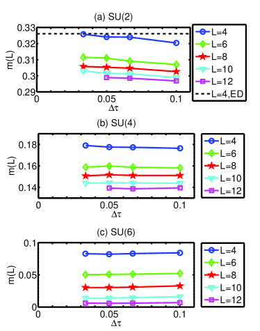
Figure 12: Scaling of the Neel moments $m(L)$ v.s. $\Delta\tau$ for the cases of SU(2), SU(4) and SU(6) shown in (a)$\sim$(c), respectively. In the case of SU(2), exact diagonalization results are also plotted as the dashed line for comparison. The parameters are $U=20$, $\beta=80$ and $h_{i_{0}j_{0}}=2$.

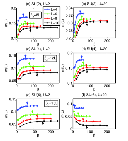
Figure 13: The scalings of the Neel moments $m(L)$ v.s. $\beta$ for the half-filled SU($2N$) Hubbard model. Lattice sizes are $L=4,6,8,10$. The interaction parameter for (a), (c), and (e) is $U=2$, and that for (b), (d), and (f) is $U=20$. Error bars of QMC data are smaller than symbols. The arrows mark the estimated convergence projection time $\beta_{c}$ of these curves. The approximate relations of $\beta_{c}$ v.s $L$ are estimated as $\beta_{c}=8L,12L$ and $15L$ for the cases of SU(2), SU(4) and SU(6), respectively.

In order to check the numeric accuracy of our simulations, we first compare our QMC results with the pinning fields in the SU(2) case with those from the exact diagonalization in the $4\times 4$ lattice. The pinning fields are applied at sites $i_{0}=(1,1)$ and $j_{0}=(2,1)$ according to Eq. 3 in the main text. In table. 1, we list the magnetic moments on sites $(1,1)$ and $(3,3)$ with different $U$’s. As $U$ goes up, the numeric errors of QMC increase, but are still less than $0.002$ even at $U=20$.

C.2 Scaling on the discrete $\Delta\tau$

For the Suzuki-Trotter decomposition defined in Eq. 8, its error is at the order of $tU^{2}(\Delta\tau)^{3}$. Such an error is most severe in the large $U$ regime, and thus we only present the scaling with respect to $\Delta\tau$ at $U=20$.

The pinning fields are chosen in the same configuration described in Eq. 3 in the main text. The distribution of $m_{i}$ is staggered with decaying magnitudes as away from two pinned sites $i_{0}$ and $j_{0}$. The weakest moments are located at the central points $(\frac{L}{2}+1,\frac{L}{2}+1)$ and $(\frac{L}{2}+2,\frac{L}{2}+1)$. The residual values at these two points are denoted as $\pm m(L)$, respectively. The long-range order can also be reached as the limit of $m(L)$ in the thermodynamic limit $L\rightarrow\infty$.

In Fig. 12, curves of the Neel moment $m(L)$ v.s. $\Delta\tau$ are plotted for the three cases of SU(2), SU(4), and SU(6), respectively. The slopes of these scaling lines are nearly independent on the lattice size $L$ for all three cases. Due to convergence of the finite $\Delta\tau$ scaling, we use the value of $\Delta\tau=0.05$ in all our simulations.

C.3 The finite $\beta$ scaling

Next we check the effect of the finite projection time $\beta$. We use the residue Neel moment $m(L)$ at the furthest points for scaling as defined in Sect. C.2. In Fig. 13, we present the scalings of the Neel moments $m(L)$ v.s. $\beta$ for different sizes $L=4,6,8$, and $10$. For each curve, we define $\beta_{c}$ as the convergence projection time after which $m(L)$ converges, and its approximate position is marked by an arrow. Here we only present the scalings at $U=2$ in the weak coupling regime and at $U=20$ in the strong coupling regime. The largest values of $\beta_{c}$ are expected in either of these two limits, which can be understood as follows: $\beta_{c}$ is determined by the finite gap of the many-body spectra. In the small $U$ regime, the finite size gap increases as increasing $U$, while in the large $U$ regime, it deceases as $U$ increases because the energy scale is controlled by the magnetic exchange scale $J\sim 4t^{2}/U$.

In the case of SU(2), the relations of $\beta_{c}$’s on $L$ are nearly the same for $U=2$ and $U=20$, which are estimated as $8L$. In the cases of SU(4) and SU(6), $\beta_{c}$’s at $U=2$ are larger than the corresponding ones at $U=20$. At $U=2$, their dependence on $L$ is estimated as $\beta_{c}\approx 12L$ for the SU(4) case and $\beta_{c}\approx 15L$ for the SU(6) case, respectively. At $U=20$, the system enters to the dimerization phase, and thus $m(L)$ is suppressed by longer projection time.

The largest size in our simulations is $L=16$. Considering the above scalings, we choose $\beta=15\times 16=240$ for all the simulations presented in the main text, which should be sufficient to obtain accurate numeric results. In particular, the major result in the main text, i.e., the non-monotonic behavior of $m(L=\infty)$ with increasing $U$ for both the SU(4) and SU(6) cases, is not an artifact from the finite projection time $\beta$.

References

- Wu (2012) C. Wu, Nat. Phys. 8, 784 (2012).
- Wu et al. (2003) C. Wu, J.-P. Hu, and S.-C. Zhang, Phys. Rev. Lett. 91, 186402 (2003).
- Wu (2006) C. Wu, Mod. Phys. Lett. B 20, 1707 (2006).
- Wu (2005) C. Wu, Phys. Rev. Lett. 95, 266404 (2005).
- Hattori (2005) K. Hattori, J. Phys. Soc. Jpn. 74, 3135 (2005).
- Lecheminant et al. (2005) P. Lecheminant, E. Boulat, and P. Azaria, Phys. Rev. Lett. 95, 240402 (2005).
- Controzzi and Tsvelik (2006) D. Controzzi and A. M. Tsvelik, Phys. Rev. Lett. 96, 097205 (2006).
- Cazalilla et al. (2009) M. A. Cazalilla, A. F. Ho, and M. Ueda, New J. Phys. 11, 103033 (2009).
- Wu et al. (2010) C. Wu, J.-P. Hu, and S.-C. Zhang, Int. J. Mod Phys B 24, 311 (2010).
- Rodríguez et al. (2010) K. Rodríguez, A. Argüelles, M. Colomé-Tatché, T. Vekua, and L. Santos, Phys. Rev. Lett. 105, 050402 (2010).
- Corboz et al. (2011) P. Corboz, A. M. Läuchli, K. Penc, M. Troyer, and F. Mila, Phys. Rev. Lett. 107, 215301 (2011).
- Hung et al. (2011) H.-H. Hung, Y. Wang, and C. Wu, Phys. Rev. B 84, 054406 (2011).
- Szirmai and Lewenstein (2011) E. Szirmai and M. Lewenstein, Europhys. Lett. 93, 66005 (2011).
- DeSalvo et al. (2010) B. J. DeSalvo et al., Phys. Rev. Lett. 105, 030402 (2010).
- Taie et al. (2010) S. Taie et al., Phys. Rev. Lett. 105, 190401 (2010).
- Krauser et al. (2012) J. S. Krauser et al., Nat. Phys. 8, 813 (2012).
- Taie et al. (2012) S. Taie, R. Yamazaki, S. Sugawa, and Y. Takahashi, Nat. Phys. 8, 825 (2012).
- Hermele et al. (2009) M. Hermele, V. Gurarie, and A. M. Rey, Phys. Rev. Lett. 103, 135301 (2009).
- Gorshkov et al. (2010) A. V. Gorshkov et al., Nat. Phys. 6, 289 (2010).
- Cai et al. (2013a) Z. Cai, H.-H. Hung, L. Wang, D. Zheng, and C. Wu, Phys. Rev. Lett. 110, 220401 (2013a).
- Messio and Mila (2012) L. Messio and F. Mila, Phys. Rev. Lett. 109, 205306 (2012).
- Cai et al. (2013b) Z. Cai, H.-H. Hung, L. Wang, and C. Wu, Phys. Rev. B 88, 125108 (2013b).
- Szirmai et al. (2011) G. Szirmai, E. Szirmai, A. Zamora, and M. Lewenstein, Phys. Rev. A 84, 011611 (2011).
- Sinkovicz et al. (2013) P. Sinkovicz, A. Zamora, E. Szirmai, M. Lewenstein, and G. Szirmai, Phys. Rev. A 88, 043619 (2013).
- Affleck (1985) I. Affleck, Phys. Rev. Lett. 54, 966 (1985).
- Arovas and Auerbach (1988) D. P. Arovas and A. Auerbach, Phys. Rev. B 38, 316 (1988).
- Affleck and Marston (1988) I. Affleck and J. B. Marston, Phys. Rev. B 37, 3774 (1988).
- Read and Sachdev (1989) N. Read and S. Sachdev, Nucl. Phys. B 316, 609 (1989).
- Read and Sachdev (1989) N. Read and S. Sachdev, Phys. Rev. Lett. 62, 1694 (1989).
- Anderson (1952) P. W. Anderson, Phys. Rev. 86, 694 (1952).
- Harada et al. (2003) K. Harada, N. Kawashima, and M. Troyer, Phys. Rev. Lett. 90, 117203 (2003).
- Kawashima and Tanabe (2007) N. Kawashima and Y. Tanabe, Phys. Rev. Lett. 98, 057202 (2007).
- Beach et al. (2009) K. S. D. Beach, F. Alet, M. Mambrini, and S. Capponi, Phys. Rev. B 80, 184401 (2009).
- Kaul and Sandvik (2012) R. K. Kaul and A. W. Sandvik, Phys. Rev. Lett. 108, 137201 (2012).
- Paramekanti and Marston (2007) A. Paramekanti and J. B. Marston, J. Phys.: Condens. Matter 19, 125215 (2007).
- Assaad (2005) F. F. Assaad, Phys. Rev. B 71, 075103 (2005).
- Note (1) The representations of SU() are classified by the Young tableau. On a bipartite lattice, the two sublattices can realize two different representations of the SU() group which are complex conjugates to each other, such that two neighboring sites can form an SU() invariant singlet. The system can be simply thought as loading fermions per site in the -sublattice and fermions per site in the -sublattice. The case of was investigated in Refs. Harada et al. (2003); Kawashima and Tanabe (2007); Beach et al. (2009); Kaul and Sandvik (2012); while the case of , which forms the self-conjugate representation, was studied in Refs. Paramekanti and Marston (2007); Assaad (2005).
- Lu (1994) J. P. Lu, Phys. Rev. B 49, 5687 (1994).
- Honerkamp and Hofstetter (2004) C. Honerkamp and W. Hofstetter, Phys. Rev. Lett. 92, 170403 (2004).
- White and Chernyshev (2007) S. R. White and A. L. Chernyshev, Phys. Rev. Lett. 99, 127004 (2007).
- Meng et al. (2010) Z. Y. Meng, T. C. Lang, S. Wessel, F. F. Assaad, and A. Muramatsu, Nature 464, 847 (2010).
- Li (2011) T. Li, Europhys. Lett. 93, 37007 (2011).
- Sorella et al. (2012) S. Sorella, Y. Otsuka, and S. Yunoki, Sci. Rep. 2, (2012).
- Hassan and Sénéchal (2013) S. R. Hassan and D. Sénéchal, Phys. Rev. Lett. 110, 096402 (2013).
- Assaad and Herbut (2013) F. F. Assaad and I. F. Herbut, Phys. Rev. X 3, 031010 (2013).
- Assaad (2012) F. F. Assaad, in KITP Conference: Exotic Phases of Frustrated Magnets (2012).
- Hirsch (1983) J. E. Hirsch, Phys. Rev. B 28, 4059 (1983).
- Note (2) See Supplementary Material [url], which includes Refs. Assaad and Evertz (2008); Wu and Zhang (2005); Schulz (1990).
- Hirsch (1985) J. E. Hirsch, Phys. Rev. B 31, 4403 (1985).
- Varney et al. (2009) C. N. Varney et al., Phys. Rev. B 80, 075116 (2009).
- Sandvik (1997) A. W. Sandvik, Phys. Rev. B 56, 11678 (1997).
- Note (3) The kinetic energy dimerization, i.e., the staggered ordering of bonding strength, is equivalent to spin-dimerization in the large- limit. In the background of half-filled Mott insulating states, the kinetic energy on each bond vanishes at the 1st order perturbation theory. Its effect begins to appear at the 2nd order as the antiferromagnetic spin-spin coupling.
- Senthil et al. (2004) T. Senthil, A. Vishwanath, L. Balents, S. Sachdev, and M. P. A. Fisher, Science 303, 1490 (2004).
- Sandvik (2007) A. W. Sandvik, Phys. Rev. Lett. 98, 227202 (2007).
- Note (4) Even though the nesting vector allows for commensurate dimerization, there appears a vertex function in the expression of its susceptibility , where is the free Green’s function. The susceptibility for the Neel ordering shares the same expression by substituting the vertex function with . The low energy density of states concentrate around points of van Hove singularity located at and at which the vertex function vanishes. Thus the angular dependences of vertex functions suppress the dimer ordering but favor Neel ordering at in the weak coupling regime.
- Assaad and Evertz (2008) F. F. Assaad and H. G. Evertz, “Computational many-particle physics,” (2008).
- (57) F. F. Assaad, arXiv:cond-mat/9806307 .
- Wu and Zhang (2005) C. Wu and S.-C. Zhang, Phys. Rev. B 71, 155115 (2005).
- Schulz (1990) H. J. Schulz, Phys. Rev. Lett. 64, 2831 (1990).
- Note (5) We thank H. H. Hung for providing the results of exact diagonalization.