Empirical Constraints on the Star Formation & Redshift Dependence of the Ly$\alpha$ ‘Effective’ Escape Fraction

Abstract

We derive empirical constraints on the volume averaged ‘effective’ escape fraction of Ly$\alpha$ photons from star forming galaxies as a function of redshift, by comparing star formation functions inferred directly from observations, to observed Ly$\alpha$ luminosity functions. Our analysis shows that the effective escape fraction increases from $f_{\rm esc}^{\rm eff}\sim 1-5\%$ at $z=0$, to $f_{\rm esc}^{\rm eff}\sim 10\%$ at $z=3-4$, and to $f_{\rm esc}^{\rm eff}=30-50\%$ at $z=6$. Our constraint at $z=6$ lies above predictions by models that do not include winds, and therefore hints at the importance of winds in the Ly$\alpha$ transfer process (even) at this redshift. We can reproduce Ly$\alpha$ luminosity functions with an $f_{\rm esc}^{\rm eff}$ that does not depend on the galaxies star formation rates ($\psi$) over up to $\sim 2$ orders of magnitude in Ly$\alpha$ luminosity. It is possible to reproduce the luminosity functions with an $f_{\rm esc}^{\rm eff}$ that decreases with $\psi$ - which appears favored by observations of drop-out galaxies - in models which include a large scatter ($\sigma~{}\hbox to0.0pt{$>$\hss}{\lower 4.30554pt\hbox{$\sim$}}1.0$ dex) in $f_{\rm esc}^{\rm eff}$, and/or in which star forming galaxies only have a non-zero $f_{\rm esc}^{\rm eff}$ for a fraction of their life-time or a fraction of sightlines. We provide a fitting formula that summarizes our findings.

1 Introduction

The Ly$\alpha$ emission line is one of the most prominent features in the intrinsic spectrum of star forming galaxies (e.g. Partridge & Peebles, 1967; Schaerer, 2003; Johnson et al., 2009). The presence of a luminous, redshifted Ly$\alpha$ line has been used to spectroscopically confirm - and find - galaxies out to $z\sim 7$ (e.g. Iye et al., 2006; Ota et al., 2010; Rhoads et al., 2012).

Ly$\alpha$ emitting galaxies (LAEs hereafter) are of interest for various reasons, including for example: (i) their continua are typically fainter than - and hence complement samples of- continuum selected (i.e. drop-out selected) galaxies; (ii) LAEs at $z>5$ provide an independent probe of the reionization epoch, as the Ly$\alpha$ line is affected by neutral intergalactic gas (e.g. Haiman & Spaans, 1999; Malhotra & Rhoads, 2004); (iii) as Ly$\alpha$ photons likely scatter through the interstellar media (ISM) of galaxies, the total distance they travel through the ISM is enhanced compared to that of continuum photons. Ly$\alpha$ photons are therefore thought to provide a sensitive probe of the dust content (and gas kinematics) of the ISM; (iv) Ly$\alpha$ selected galaxies will be used to probe the equation of state of the dark energy at $z=1.9-3.5$ by the HETDEX experiment (Hill et al., 2008).

The main uncertainty that affects interpretations of Ly$\alpha$ observations of LAEs relates to the complex radiative transfer of Ly$\alpha$ photons through both the ISM, the circum galactic medium (CGM), and intergalactic medium (IGM, e.g. Zheng et al., 2010; Dijkstra & Kramer, 2012; Verhamme et al., 2012; Laursen et al., 2012; Cantalupo et al., 2012; Jeeson-Daniel et al., 2012). Moreover, these processes are not independent: radiative transfer at the ISM-level affects how the radiative transfer proceeds at the intergalactic level. In recent years Ly$\alpha$ RT has been modeled on all these scales, usually by combining simulated galaxies with Ly$\alpha$ radiative transfer calculations (e.g Tasitsiomi, 2006; Laursen & Sommer-Larsen, 2007; Barnes et al., 2011; Verhamme et al., 2012; Yajima et al., 2012). These calculations are extremely difficult to carry out from first principles (see Dijkstra & Kramer 2012), and ultimately must be constrained by observations.

The goal of this paper is to provide empirical (i.e. based purely on observations) constraints on the dependence of the effective escape fraction of Ly$\alpha$ photons, $f_{\rm esc}^{\rm eff}\equiv L_{\alpha}/L_{\alpha,\rm int}$, where $L_{\alpha}$ ($L_{\alpha,\rm em}$) denotes the observed (intrinsic) Ly$\alpha$ luminosity. Our goal is to constrain $f_{\rm esc}^{\rm eff}$ as a function of redshift (as in Hayes et al., 2011; Blanc et al., 2011). Furthermore, we investigate whether $f_{\rm esc}^{\rm eff}$ depends on the star formation rate of galaxies. Previous works by Hayes et al. (2011) and Blanc et al. (2011) constrained the volume averaged effective escape fraction $f_{\rm esc}^{\rm eff}$ by comparing the star formation rate density, $\dot{\rho}_{*}$, inferred from the observed Ly$\alpha$ luminosity density, to $\dot{\rho}_{*}$ inferred from other observations. This method is highly non-trivial, because Ly$\alpha$ observations only detect galaxies for which $f_{\rm esc}^{\rm eff}$ exceeds some star formation rate-dependent value (at very low star formation rates, the Ly$\alpha$ flux falls below the detection threshold even when all Ly$\alpha$ photons made it to the observer), and one must attempt to account for this. For example, Hayes et al. (2011) use UV-luminosity functions of drop-out galaxies to estimate the appropriate value for $\dot{\rho}_{*}$ at $z~{}\hbox to0.0pt{$>$\hss}{\lower 4.30554pt\hbox{$\sim$}}2.5$, and a significant part of their analysis is devoted to choosing the proper lower integration limit when integrating over the UV-luminosity function. Our method uses star formation rate functions to estimate $f_{\rm esc}^{\rm eff}$. We show that this allows for more direct constraints which circumvent the difficulties associated with choosing such integration limits.

The outline of this paper is as follows: We describe in § 2 how we combine observations of Ly$\alpha$ luminosity functions of LAEs with observations of star formation functions, to put constraints on the effective escape fraction of Ly$\alpha$ photons, $f_{\rm esc}^{\rm eff}$. We present our main results in § 3 before presenting our conclusions in § 5.

2 Empirical Constraints on the Ly$\alpha$ Effective Escape Fraction

Ly$\alpha$ photons - just as H$\alpha$ photons - are emitted following recombination events in HII regions, and closely trace ongoing star formation. The H$\alpha$ luminosity of a galaxy is related to its star formation rate, denoted with $\psi$, as $L_{{\rm H}\alpha}=1.2\times 10^{41}\times(\psi/[{\rm M}_{\odot}\hskip 2.84526pt{\rm yr}^{-1}])$ erg s^-1 (Kennicutt, 1998, this conversion assumes a Salpeter IMF in the mass range 0.1-100 $M_{\odot}$). The intrinsic Ly$\alpha$ luminosity, denoted with $L_{\alpha,{\rm int}}$, is $\sim 8\times$ larger than the H$\alpha$ luminosity (for case-B recombination and $T=10^{4}$ K, e.g. Hayes et al. 2011), and we have

$$L_{\alpha,{\rm int}}=k\times\Big{(}\frac{\psi}{M_{\odot}\hskip 2.84526pt{\rm yr}^{-1}}\Big{)},$$ (1)

where $k=10^{42}$ erg s^-1. The factor $k$ can be higher (or lower) by a factor of $\sim 2$ depending on the assumed IMF, and/or stellar metallicity. In the extreme case of a top-heavy IMF and zero-metallicity stars, the factor $k$ can be as high as $k\approx 10$ (Raiter et al., 2010). Our constraints on $f_{\rm esc}^{\rm eff}$ scale with our assumed $k$ as $f_{\rm esc}^{\rm eff}\propto k^{-1}$. The ‘observed Ly$\alpha$ luminosity’, defined as the observed flux multiplied by $4\pi d^{2}_{\rm L}(z)$ ($d_{\rm L}(z)$ denotes the luminosity distance out to redshift $z$), is

$$L_{\alpha}=f_{\rm esc}^{\rm eff}(\psi,z)\times L_{\alpha,{\rm int}},$$ (2)

where $f_{\rm esc}^{\rm eff}(\psi,z)$ denotes the effective escape fraction of Ly$\alpha$ photons.

We constrain the parameter $f_{\rm esc}^{\rm eff}(\psi,z)$ by comparing observed Ly$\alpha$ luminosity functions to observationally inferred star formation functions: the Ly$\alpha$ luminosity function, denoted by $\frac{dn}{d\log L_{\alpha}}d\log L_{\alpha}$, measures the comoving number density of galaxies with (the logarithm of their) Ly$\alpha$ luminosities in the range $\log L_{\alpha}\pm d\log L_{\alpha}/2$. The star formation function, denoted with $\frac{dn}{d\log\psi}d\log\psi$ measures the comoving number density of galaxies that are forming stars at rate (whose logarithm is) in the range $\log\psi\pm d\log\psi/2$. We describe the star formation functions used in our analysis, and how we convert these into Ly$\alpha$ luminosity functions in § 2.1. This conversion depends on $f_{\rm esc}^{\rm eff}(\psi,z)$, and we use observed Ly$\alpha$ luminosity functions to obtain constraints in § 3.

2.1 Star Formation Functions

Star formation functions can be described by Schechter functions:

$$\frac{dn}{d\log\psi}={\rm ln}\hskip 2.84526pt10\times\psi\times\frac{\Phi_{*}}{\psi_{*}}\Big{(}\frac{\psi}{\psi_{*}}\Big{)}^{-\alpha}\exp(-\psi/\psi_{*}).$$ (3)

We adopt the redshift dependent Schechter function parameters from Smit et al. (2012, their Table 3). Our results are insensitive to this choice (see § 4.3).

In the absence of scatter, there is a one-to-one relation between $\psi$ and $L_{\alpha}$. The Ly$\alpha$ luminosity functions then relate to the star formation functions as

$$\frac{dn}{d\log L_{\alpha}}=\frac{dn}{d\log\psi}\frac{d\log\psi}{d\log L_{\alpha}}=\frac{dn}{d\log\psi}\Big{|}_{\psi=L_{\alpha}/(kf_{\rm esc}^{\rm eff})},$$ (4)

where in the last equality we used Eq 1 and Eq 2.

In reality we do not expect each galaxy that forms stars at some rate $\psi$ to have exactly the same $f_{\rm esc}^{\rm eff}$. It is therefore reasonable to study models in which we assume that there is a dispersion (or scatter) in $f_{\rm esc}^{\rm eff}$ at a fixed $\psi$. In the presence of scatter, we generally have

$$\frac{dn}{d\log L_{\alpha}}=\int_{-\infty}^{\infty}d\log\psi\hskip 2.84526pt\frac{dn}{d\log\psi}P(\log L_{\alpha}|\log\psi)$$ (5)

where $P(\log L_{\alpha}|\log\psi)d\log L_{\alpha}$ denotes the probability that a galaxy that is forming stars at a rate $\psi$ has a Ly$\alpha$ luminosity in the range $\log L_{\alpha}\pm d\log L_{\alpha}/2$. We assume that the effective escape fraction $f_{\rm esc}^{\rm eff}$ has a scatter that is described by a (truncated) log-normal distribution. That is,

$$P(\log L_{\alpha}|\log\psi)\equiv\frac{dP}{d\log L_{\alpha}}=\frac{dP}{d\log f_{\rm esc}^{\rm eff}}\Big{|}_{f_{\rm esc}^{\rm eff}=L_{\alpha}/(k\psi)}=$$

$$=\left\{\begin{array}[]{ll}\frac{\mathcal{N}}{\sqrt{2\pi}\sigma}\exp\Big{(}\frac{-(\log f_{\rm esc}^{\rm eff}-\langle\log f_{\rm esc}^{\rm eff}\rangle)^{2}}{2\sigma^{2}}\Big{)}&f_{\rm esc}^{\rm eff}\leq 1\\ 0&f_{\rm esc}^{\rm eff}>1\end{array}\right.,$$

where $\mathcal{N}$ denotes a factor that ensures that the function $dP/d\log f_{\rm esc}^{\rm eff}$ is normalized.

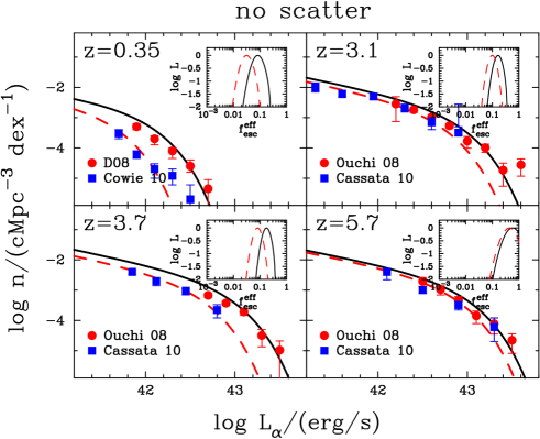
Figure 1: The Figure compares observed Ly$\alpha$ luminosity functions (indicated by the data points) of LAEs at $z=0.35$ (upper left), $z=3.1$ (upper right), $z=3.7$ (lower left), and $z=5.7$ (lower right) with model predictions under the assumption that there is a one-to-one relation between star formation rate $\psi$ and observed Ly$\alpha$ luminosity $L_{\alpha}$ (see Eq 4, i.e. there is no scatter in $f_{\rm esc}^{\rm eff}$), for the best-fit observed Ly$\alpha$ fraction, $f_{\rm esc}^{\rm eff}$, (as black solid lines and red dashed lines, see text). The insets show the likelihood $\mathcal{L}[f_{\rm esc}^{\rm eff}]$ as a function of $f_{\rm esc}^{\rm eff}$. This Figure illustrates that the models reproduce the Ly$\alpha$ luminosity functions well, except at the bright end (which may be contaminated by low luminosity AGN, see Ouchi et al. 2008). It is worth pointing out that $f_{\rm esc}^{\rm eff}$ is independent of $\psi$ in our models.

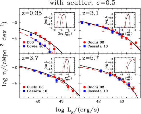
Figure 2: Same as Figure 1, but for models in which we assume that there is a dispersion in $f_{\rm esc}^{\rm eff}$, described by a log-normal distribution with a standard deviation of $\sigma=0.5$, at a fixed $\psi$. This Figure shows that a dispersion in $f_{\rm esc}^{\rm eff}$ flattens the predicted Ly$\alpha$ luminosity functions, which improves the agreement with the data at $z=0.35$ and at high $L_{\alpha}$. These models obtain constraints from different datasets that agree better with each other.

2.2 Constraining the Effective Escape Fraction.

We first assume that $f_{\rm esc}^{\rm eff}(z,\psi)=f_{\rm esc}^{\rm eff}(z)$. That is, we first assume that $f_{\rm esc}^{\rm eff}$ is independent of the star formation rate $\psi$. We make this assumption because we will show later that the Ly$\alpha$ luminosity functions are - surprisingly - consistent with this assumption.

Our analysis focusses on the Ly$\alpha$ luminosity functions centered on $z=0.35$ from Deharveng et al. (2008, red filled circles) and Cowie et al. (2010, blue filled squares), $z=3.1$, $z=3.7$, and $z=5.7$ from Ouchi et al. (2008, red filled circles) and Cassata et al. (2011, blue filled squares). At each redshift, we compute the posterior probability for a range of $f_{\rm esc}^{\rm eff}$ as $P(f_{\rm esc}^{\rm eff})\propto\int d^{3}{\bf X}\hskip 2.84526pt\mathcal{L}[f_{\rm esc}^{\rm eff}]P(f_{\rm esc}^{\rm eff})P_{\rm s}({\bf X})$, where $\mathcal{L}[f_{\rm esc}^{\rm eff}]=\exp[-0.5\chi^{2}]$ denotes the likelihood, in which $\chi^{2}=\sum_{i}^{N_{\rm data}}({\rm model}_{i}-{\rm data}_{i})^{2}/\sigma^{2}_{i}$. The function $P(f_{\rm esc}^{\rm eff})\equiv 1$ denotes the prior probability distribution for $f_{\rm esc}^{\rm eff}$: i.e. we assume no prior knowledge of $f_{\rm esc}^{\rm eff}$. We stress however that our results do not depend on our choice of prior.

Finally, the vector ${\bf X}$ contains the three Schechter function parameters ${\bf X}^{T}=$($\alpha,\psi_{*},\Phi_{*}$). The function $P_{\rm s}({\bf X})$ describes the prior probability for having any combination of parameters: we assumed that $P_{\rm s}({\bf X})$ is a multivariate Gaussian, i.e. $P_{\rm s}({\bf X})=\mathcal{N}\exp\Big{[}-\frac{1}{2}({\bf X}-{\bf\mu}_{X})^{T}{\bf C}^{-1}({\bf X}-{\bf\mu}_{X})\Big{]}$, where $\mathcal{N}$ denotes the normalization factor. The vector ${\bf\mu}_{X}$ contains the best fit values for each of the parameters. The covariance matrix ${\bf C}$ contains the measured uncertainties on the parameters (the most likely values and their uncertainties were taken from Smit et al. 2012).

3 Results

3.1 No Scatter

Figure 1 shows four panels, each of which corresponds to one redshift bin. The observed Ly$\alpha$ luminosity functions that we used in our analysis are shown as the datapoints. The inset in each panel shows $\mathcal{L}[f_{\rm esc}^{\rm eff}]$ as a function of $f_{\rm esc}^{\rm eff}$. These panels contain two lines, both of which were obtained by fitting to a single data set. For example, we obtained the black solid line (red dashed line) in the $z=0.35$ panel by fitting to the data from Deharveng et al. (2008) (Cowie et al. 2010). At each redshift, we show the model luminosity functions for which both $\mathcal{L}[f_{\rm esc}^{\rm eff}]$-curves are maximized, using the same line color and style.

The upper left panel shows that the data from Deharveng et al. (2008) translates to $f_{\rm esc}^{\rm eff}=8.5\pm 3\%$, while the data from Cowie et al. (2010) implies $f_{\rm esc}^{\rm eff}=3^{+2}_{-1}\%$ at $z=0.35$. Here the errorbars denote 68% confidence levels, where we use the so-called ‘shortest interval’ method (see Andrae, 2010, and references therein) to determine the confidence intervals. The upper right panel shows that the effective escape fraction increases to $f_{\rm esc}^{\rm eff}=17\pm 5\%$ [$f_{\rm esc}^{\rm eff}=10\pm 3\%$] for the Ouchi et al. (2008) [Cassata et al. (2010)] data at $z=3.1$, and to $f_{\rm esc}^{\rm eff}=17^{+6}_{-4}\%$ [$f_{\rm esc}^{\rm eff}=8\pm 3\%$] for the Ouchi et al. (2008) [Cassata et al. 2010] data at $z=3.7$. Finally, we find that the effective escape fraction increases to $f_{\rm esc}^{\rm eff}=57^{+34}_{-21}\%$ [$f_{\rm esc}^{\rm eff}=44^{+28}_{-22}\%$] for the Ouchi et al. (2008) data [Cassata et al. (2010)] at $z=5.7$.

Our quoted uncertainties are statistical only, and do not take into account systematic uncertainties associated with the determination of observed Ly$\alpha$ luminosity functions. The different constraints we obtain on $f_{\rm esc}^{\rm eff}$ from different data-sets may reflect these systematic uncertainties: in particular, at $z\geq 3.1$ the data from Ouchi et al. (2008) derive from a narrow-band survey for LAEs, while the data from Cassata et al. (2010) derive from a deep spectroscopic survey (see § 4.3 for a more detailed discussion of systematic uncertainties).

Figure 1 shows that our models reproduce the individual datasets of observed Ly$\alpha$ luminosity functions well. Different datasets can result in slightly different constraints on $f_{\rm esc}^{\rm eff}$. It is striking that at $z\geq 3.1$ (especially $z=3.1$ and $z=5.7$), a $\psi$-independent $f_{\rm esc}^{\rm eff}$ reproduces the observations well over up to two orders Ly$\alpha$ luminosity, and therefore $\psi$. If anything, our models do not produce enough bright LAEs, which could be solved by having $f_{\rm esc}^{\rm eff}$ increase with $\psi$. Note however, that Ouchi et al. (2008) point out that the bright end (i.e. at $\log L_{\alpha}~{}\hbox to0.0pt{$>$\hss}{\lower 4.30554pt\hbox{$\sim$}}43.4$) may be contaminated by low luminosity AGN. The only data-set that we cannot reproduce well is that of Cowie et al. (2010): our model predicts significantly fewer LAEs than their two data-points at $\log L_{\alpha}~{}\hbox to0.0pt{$>$\hss}{\lower 4.30554pt\hbox{$\sim$}}42.3$. This discrepancy could again be (partially) resolved by having $f_{\rm esc}^{\rm eff}$ increase with $\psi$. As we show below (in § 3.2), we also significantly improve the agreement with the data when we introduce a scatter in $f_{\rm esc}^{\rm eff}$.

3.2 With Scatter

Figure 2 shows the same as Figure 1, but here the models include a dispersion in $f_{\rm esc}^{\rm eff}$ (Eq 5), which is described by a (truncated) log-normal distribution with a standard deviation of $\sigma=0.5$. This choice for $\sigma$ is a bit arbitrary, but can be justified by the work of Dijkstra & Westra (2010), who found that the ratio of the Ly$\alpha$ to the UV-derived star formation rate can be described by a log-normal distribution with $\sigma=0.4$. We stress that changes to our main results are insignificant, even if we adopted $\sigma=1.0$.

Figure 2 shows that a dispersion in $f_{\rm esc}^{\rm eff}$ flattens the predicted luminosity functions, and smoothens out the sharp-turnover in the predicted luminosity function. Both these changes help to improve the fit to the data at $z=0.35$ (and also at the highest $L_{\alpha}$ data point at $z=3.1$). Importantly, these models obtain constraints from different datasets that agree better with each other: for example, the best-fit models to the data from Ouchi et al. (2008) also provide decent fits to the data from Cassata et al. (2010).

In spite of the flattening of the predicted luminosity functions, these models still reproduce the data with an $\langle\log f_{\rm esc}^{\rm eff}\rangle$ that is independent of $\psi$. It is only when we adopt $\sigma~{}\hbox to0.0pt{$>$\hss}{\lower 4.30554pt\hbox{$\sim$}}1.0$, that the predicted luminosity functions become flatter than the observations. Garel et al. (2012) have recently predicted that the scatter in $f_{\rm esc}^{\rm eff}$ increases with $\psi$, and that may be even larger than this at $\psi~{}\hbox to0.0pt{$>$\hss}{\lower 4.30554pt\hbox{$\sim$}}20\hskip 2.84526ptM_{\odot}$ yr^-1. For models that include this large scatter, the data would require $\langle\log f_{\rm esc}^{\rm eff}\rangle$ to decrease with $\psi$. Such a requirement would be expected given observations of drop-out galaxies, which show evidence that the fraction of continuum selected galaxies that have ‘strong’ Ly$\alpha$ emission lines increases towards lower UV-luminosities (e.g. Stark et al., 2010). This suggests that Ly$\alpha$ photons have an easier time escape from galaxies with lower UV luminosities, and therefore likely from galaxies with lower star formation rates $\psi$.

The insets of Figure 2 show $\mathcal{L}(\langle\log f_{\rm esc}^{\rm eff}\rangle)$. For example, the inset in the upper right panel shows that the best-fit $\langle\log f_{\rm esc}^{\rm eff}\rangle$ at $z=3.1$ is $10^{\langle\log f_{\rm esc}^{\rm eff}\rangle}\sim 0.06-0.1$, which lie a factor of $\sim 1.7$ below the best-fit $f_{\rm esc}^{\rm eff}$ we derived for the model with no scatter. The best-fit values of $\langle\log f_{\rm esc}^{\rm eff}\rangle$ depend on the choice of $\sigma$: the larger $\sigma$, the smaller $\langle f_{\rm esc}^{\rm eff}\rangle$. The reason for this reduction is that at fixed $\langle\log f_{\rm esc}^{\rm eff}\rangle$, increasing $\sigma$ increases the expectation value $E(f_{\rm esc}^{\rm eff})$, which is given by $E(f_{\rm esc}^{\rm eff})=\int_{0}^{1}df_{\rm esc}^{\rm eff}\hskip 2.84526ptf_{\rm esc}^{\rm eff}\frac{dP}{df_{\rm esc}^{\rm eff}}$. We have verified that this best-fit expectation value $E(f_{\rm esc}^{\rm eff})$ barely depends on our choice of $\sigma$.

We now practically have three ‘measures’ of $f_{\rm esc}^{\rm eff}$ (namely $f_{\rm esc}^{\rm eff}$, $\langle\log f_{\rm esc}^{\rm eff}\rangle$, and $E(f_{\rm esc}^{\rm eff})$), which may be a bit confusing. We have therefore briefly summarized the meaning of these symbols in Table 1.

Table 1: Summary of ‘Different’ Measures of $f_{\rm esc}^{\rm eff}$.

. symbol meaning $f_{\rm esc}^{\rm eff}$ effective escape fraction of Ly$\alpha$ of a galaxy $\langle\log f_{\rm esc}^{\rm eff}\rangle$ mean of log $f_{\rm esc}^{\rm eff}$ in a lognormal PDF (Eq 2.1) $E(f_{\rm esc}^{\rm eff})$ expectation value of $f_{\rm esc}^{\rm eff}$ for models with a lognormal PDF

3.3 Comparing our $f_{\rm esc}^{\rm eff}(z)$ with Previous Works

We compare our inferred redshift evolution of $f_{\rm esc}^{\rm eff}(z)$ to the power-law fitting function from Hayes et al. (2011) in Figure 3. The filled symbols represent the constraints on $f_{\rm esc}^{\rm eff}$ that we obtained for the ‘no-scatter’ models in § 3.1. The open symbols represent our constraints on the best-fit expectation value $E(f_{\rm esc}^{\rm eff})$ (these constraints do not depend on our adopted $\sigma$). We have off-set these data points by $\Delta z=0.2$ for clarity. At each redshift, we have two data points which correspond to different data sets. Including scatter reduces the expectation value of $f_{\rm esc}^{\rm eff}$ compared to models that have no scatter, typically by about $\sim 1\sigma$. The reduction is a bit larger at $z=0.35$. However, here we point out that the models that do not include scatter had difficulties fitting the data to begin with, and the constraints that we inferred from these models were likely less reliable.

Figure 3 shows that our best-fit values are consistent with Hayes et al. (2011) at $z\geq 3.1$, albeit on the high end of their quoted range. At $z=0.35$, our constraints on $f_{\rm esc}^{\rm eff}$ lie significantly higher than those of Hayes et al. (2011), who found $f_{\rm esc}^{\rm eff}=1.3\pm 0.9\%$ using the data from Deharveng et al. (2008), and $f_{\rm esc}^{\rm eff}=0.3\pm 0.2\%$ using the data from Cowie et al. (2010). These values would clearly not allow us to reconstruct the observed Ly$\alpha$ luminosity functions. Our constraint at $z=0.35$ is in better agreement with the ‘transition model’ fit by Blanc et al. (2011). Their fit is represented by the red dotted line (which shows the ‘no LF integration limit’ fit), which predicts $f_{\rm esc}^{\rm eff}\sim 2\%$ at $z=0.35$. This same fit gives slightly lower values for $f_{\rm esc}^{\rm eff}$ at $1~{}\hbox to0.0pt{$<$\hss}{\lower 4.30554pt\hbox{$\sim$}}z~{}\hbox to0.0pt{$<$\hss}{\lower 4.30554pt\hbox{$\sim$}}3.5$ than ours.

A possible explanation for the lower preferred values for $f_{\rm esc}^{\rm eff}$ at $z=0.35$ by Hayes et al. (2011) is that they compare the observed Ly$\alpha$ luminosity density to a total star formation rate density of $\dot{\rho}_{*}\sim 30\times 10^{-3}$ M_⊙ yr^-1 cMpc^-3. This value corresponds to the total integrated star formation rate density (see Table 1 of Bothwell et al., 2011). Bothwell et al. (2011) show that galaxies with $\psi~{}\hbox to0.0pt{$>$\hss}{\lower 4.30554pt\hbox{$\sim$}}10$ M_⊙ yr^-1 account only for $\sim 20\%$ of $\dot{\rho}_{*}$. If we consider an extreme example in which all galaxies with $\psi<10$ M_⊙ yr^-1 have $f_{\rm esc}^{\rm eff}=3\%$, then their observed Ly$\alpha$ luminosity would be $L_{\alpha}\sim 3\times 10^{41}$ erg s^-1, which lies below the minimum detectable Ly$\alpha$ luminosity. The luminosity function presented by Cowie et al. (2010) is therefore consistent with all galaxies $\psi<10$ M_⊙ yr^-1 having $f_{\rm esc}^{\rm eff}=3\%$. Even if all galaxies with $\psi>10$ M_⊙ yr^-1 would have $f_{\rm esc}^{\rm eff}=0$, then $f_{\rm esc}^{\rm eff}$ averaged over the population as a whole would be $\sim 2.4\%$, which is almost an order of magnitude higher than the value reported by Hayes et al. (2011). While the example we discussed here is clearly not realistic, it nevertheless shows that for very small $f_{\rm esc}^{\rm eff}$, large systematic uncertainties may be associated with estimating $f_{\rm esc}^{\rm eff}$ by comparing an observed Ly$\alpha$ luminosity density to a star formation rate density. Another way to phrase this is that for very small $f_{\rm esc}^{\rm eff}$, existing observations probe luminosities that are likely close to (or even larger than) $L_{*}$ in the Ly$\alpha$ luminosity function. In these cases, it is difficult and uncertain to estimate the Ly$\alpha$ luminosity density in faint, undetected sources.

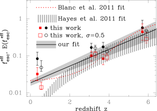
Figure 3: This Figure compares our constraints on $f_{\rm esc}^{\rm eff}$ with the analytic fitting formula provided by Hayes et al. (2011, indicated by the black shaded region). The filled symbols (off-set by $\Delta z=0.2$ for clarity) represent the constraints on $f_{\rm esc}^{\rm eff}$ for the ‘no-scatter’ models. The open symbols represent our constraints on the expectation values of $E(f_{\rm esc}^{\rm eff})$ for our models that include scatter. At each redshift, we have two data points which correspond to different data sets. The grey region represents our fitting formula (Eq 8) and its uncertainties. Our work is consistent with Hayes et al. (2011), except at $z=0.35$ where our inferred $f_{\rm esc}^{\rm eff}$ is higher, which is likely related to systematic uncertainties (see text). Our constraint at this redshift is in better agreement with that given by the ‘transition model’ fit of Blanc et al. (2011, indicated by the red dotted line).

We have also indicated a (ad-hoc) fitting formula that we found to capture the redshift evolution of our inferred $f_{\rm esc}^{\rm eff}$ reasonably well:

$$f_{\rm esc}^{\rm eff}(z,\psi)=\exp(-\tau_{\rm eff}),\hskip 2.84526pt\hskip 2.84526pt\tau_{\rm eff}=a_{1}+a_{2}z$$ (8)

, where $a_{1}=4.0\pm 0.16$ and $a_{2}=-0.52\pm 0.05$. We obtain best fit values for $a_{1}$ and $a_{2}$ by minimizing $\chi^{2}$, which we compute using all 16 data points shown in Figure 3. The redshift evolution of $f_{\rm esc}^{\rm eff}$ for the best fit combination of $a_{1}$ and $a_{2}$ is represented by the black solid line in Figure 2. The upper/lower boundary of the grey region represents our fitting formula when we simultaneously subtract/add $\sigma/\sqrt{2}$ to both $a_{1}$ and $a_{2}$. Here, uncertainties on the parameters $a_{1}$ and $a_{2}$ represent marginalized $1\sigma$ uncertainties. The fitting formula Eq. 8 captures our main results well, and further ‘predicts’ that $f_{\rm esc}^{\rm eff}\sim 5^{+2}_{-1}\%$ at $z=2$, which is consistent with Hayes et al. (2010) who found $f_{\rm esc}^{\rm eff}=5.3\pm 3.8\%$ by comparing Ly$\alpha$ to H$\alpha$ luminosity functions. We have also applied our analysis to the more recent $z\sim 1$ data of Barger et al. (2012, not shown here), and found $f_{\rm esc}^{\rm eff}=5\pm 1\%$ for the ‘no scatter case’, which is also captured reasonably well by our fitting formula.

4 Discussion

4.1 ‘Effective Escape’ Fraction vs. ‘Escape’ Fraction

We explicitly differentiate between the term ‘escape’ fraction and ‘effective escape’ fraction, because these two quantities can take on very different values. In theoretical calculations that follow the transport of Ly$\alpha$ photons through a dusty medium, it is straightforward to compute the fraction of photons that are not absorbed by dust, and hence ‘escape’ (e.g. Neufeld, 1990; Hansen & Oh, 2006; Laursen & Sommer-Larsen, 2007; Yajima et al., 2012; Laursen et al., 2012; Yajima et al., 2013). However, a large fraction of Ly$\alpha$ photons that escape from this medium can scatter in the surrounding circum-galactic and/or intergalactic medium and give rise to a low surface brightness Ly$\alpha$ glow around galaxies (e.g. Dijkstra et al., 2007; Zheng et al., 2010; Laursen et al., 2011; Zheng et al., 2011; Steidel et al., 2011; Jeeson-Daniel et al., 2012). The surface brightness of this scattered radiation is typically much fainter than can be observed, and this Ly$\alpha$ radiation would effectively be lost in observations. For example, Zheng et al. (2010) find that Ly$\alpha$ scattering in the ionized IGM at $z=5.7$ rendered $80-95\%$ of all emitted Ly$\alpha$ radiation undetectable (consistent with the other studies, see § 4.4). There is no dust in their simulations, and the escape fraction of Ly$\alpha$ photons is $100\%$. In contrast, the effective escape fraction would only be $f_{\rm esc}^{\rm eff}\sim 5-20\%$.

There is also observational evidence for the existence of spatially extended low surface brightness Ly$\alpha$ emission around galaxies (e.g. Fynbo et al., 2001; Ostlin et al., 2009; Rauch et al., 2008; Steidel et al., 2011; Matsuda et al., 2012; Hayes et al., 2013). Steidel et al. (2011) detected spatially extended Ly$\alpha$ emission after stacking Ly$\alpha$ observations on 92 $z\sim 2.6$ LBGs, which allowed them to probe Ly$\alpha$ emission down to $\sim 10$ times fainter surface brightness levels. The total flux in their spatially extended halos significantly exceeded the total Ly$\alpha$ flux coming directly from their galaxies. The observations by Steidel et al. (2011) imply that the escape fraction of Ly$\alpha$ photons can exceed the effective escape fraction significantly for surface brightness thresholds that are typical for current observations. Similarly, Matsuda et al. (2012) detected Ly$\alpha$ halos around $z=3.1$ LAEs and found that the size of the halos (at fixed UV-luminosity of the LAEs) increases with local density (measured by the number density of LAEs). This dependence may help explain why other groups have not detected spatially extended Ly$\alpha$ halos around LAEs (e.g. Feldmeier et al. 2013). In any case, the possibility that there is more Ly$\alpha$ flux in diffuse Ly$\alpha$ halos than in a compact source illustrates that the effective escape fraction - and previous determinations of this quantity - depend on the surface brightness threshold of the survey of interest (or the size of the photometric aperture in fixed aperture photometry), while the escape fraction does not (also see Yajima et al., 2012).

The universal usage of the term escape fraction complicates comparisons between different studies: for example, Yajima et al. (2013) compute true Ly$\alpha$ escape fractions in simulated galaxies as a function of redshift. Similarly, semi-analytic studies that model LAEs at $z=3-6$ (e.g. Kobayashi et al., 2007; Dayal et al., 2011; Shimizu et al., 2011; Forero-Romero et al., 2011) introduce an escape fraction, which corresponds to a true escape fraction. Caution must be exercised when comparing these escape fractions to the observationally inferred effective escape fractions (as in Hayes et al. 2011, Blanc et al. 2011, and in this paper). Moreover, in some (but not all) studies the constraints on $f_{\rm esc}$ (and/or $f_{\rm esc}^{\rm eff}$) involve a ‘correction’ for scattering in the IGM. We stress that this correction is highly uncertain, as it depends on the radiative transfer at the interstellar and circum-galactic level (see § 1).

4.2 Comparison to Previous Works

We already compared our results to those obtained by Hayes et al. (2011, and also Blanc et al. 2010). Our approach, in which we use star formation functions and Ly$\alpha$ luminosity functions to constrain $f_{\rm esc}^{\rm eff}$, is similar to that adopted in theoretical studies. For example, Le Delliou et al. (2006) use semi-analytic models - while e.g. Nagamine et al. (2010) use hydrodynamical simulations - to generate star formation functions, and then use Ly$\alpha$ luminosity functions to constrain $f_{\rm esc}^{\rm eff}$ at $z=3-6$. Importantly, the models that are used to generate the theoretical star formation functions are typically constrained by observations. However, these (almost the same) observations can be converted directly into star formation functions, i.e. without generating the intermediate theoretical model. Indeed, our method completely circumvents this intermediate step. The fact that we can side-step this (substantial) part of the calculations allow us to more efficiently explore a larger suite of models for $f_{\rm esc}^{\rm eff}$, and to explore the impact of uncertainties with the observationally inferred star formation functions on our results.

Our results are broadly consistent with these previous theoretical studies: Nagamine et al. (2010) find that $f_{\rm esc}^{\rm eff}=0.1$ at $z=3.1$, which is in excellent agreement with our results. Nagamine et al. (2010) find $f_{\rm esc}^{\rm eff}=0.15$ at $z=6$, which is a factor of $\sim 2-3$ lower than what we find. The origin of this difference is unclear, but the lower right panel of Figure 2 shows that the value preferred by Nagamine et al. (2010) ($10^{\langle\log f_{\rm esc}^{\rm eff}\rangle}=0.15$) is not ruled out at great significance. Le Delliou et al. (2006) find $f^{\rm eff}_{\rm esc}\sim 0.02$ at $z=3-6$. However, a redshift-dependent fraction of stars form in bursts with a top-heavy IMF for which $k\sim 10$ (see § 2) in their models. Hayes et al. (2011) show that if this top-heavy IMF is replaced with a standard Salpeter IMF, that then the constraints obtained by Le Delliou et al. (2006) agree well with Nagamine et al. (2010) at $z=3-6$.

Finally, Nagamine et al. (2010) showed that while their models with a constant $f_{\rm esc}^{\rm eff}$ fit the data well (in good agreement with our work), they obtain better fits using so-called ‘duty cycle’ models, in which $\frac{dn}{d\log L_{\alpha}}=\epsilon_{\rm DC}\frac{dn}{d\log\psi}\big{|}_{\psi=L_{\alpha}/kf_{\rm esc}^{\rm eff}}$. These models represent a scenario in which star forming galaxies only have non-zero $f_{\rm esc}^{\rm eff}$ for a fraction $\epsilon_{\rm DC}$ of their lifetimes. We note that this may also represent a scenario in which Ly$\alpha$ escapes anisotropically from galaxies, and in which $f_{\rm esc}^{\rm eff}>0$ only along a fraction $\epsilon_{\rm DC}$ of the sightlines from them. The duty cycle parameter $\epsilon_{\rm DC}$ can also be incorporated in the $f_{\rm esc}^{\rm eff}$-PDF, simply by adding a Dirac-delta function at $f_{\rm esc}^{\rm eff}=0$ (after which we must renormalize the full-PDF). We have repeated our analysis including a duty cycle of $\epsilon_{\rm DC}=0.25$ into our $f_{\rm esc}^{\rm eff}$-PDF, and found that these models flatten the predicted luminosity functions, similarly to models with a non-zero scatter in $f_{\rm esc}^{\rm eff}$. These ‘duty-cycle model’ therefore provide somewhat better fits to the luminosity functions (for models with $\sigma=0$), mostly because they improve the fits at the bright ends (just as our models with $\sigma=0.5$), in agreement with Nagamine et al. (2010). Moreover, the best-fit expectation values of $f_{\rm esc}^{\rm eff}$ in these duty cycle models are consistent with our those obtained previously.

4.3 Model Uncertainties

A potential caveat is that (some of) our adopted Ly$\alpha$ luminosity functions were constructed from narrow-band surveys. Such surveys do not only impose a Ly$\alpha$ flux cut, but in practice also a cut in Ly$\alpha$ equivalent width (EW). For example, Ouchi et al. (2008) adopt color-color criteria to select LAEs at $z=3.1$ that translate (roughly) to EW$~{}\hbox to0.0pt{$>$\hss}{\lower 4.30554pt\hbox{$\sim$}}64$ Å. We may worry that this data-set therefore misses a significant fraction of Ly$\alpha$ emitting galaxies. In practise however, the equivalent width cut does not appear to affect determinations of the Ly$\alpha$ luminosity functions: Gronwall et al. (2007) present a luminosity function at $z=3.1$ that agrees well with Ouchi et al. (2008), even though they effectively apply a different EW-cut of EW$~{}\hbox to0.0pt{$>$\hss}{\lower 4.30554pt\hbox{$\sim$}}20$ Å. Moreover, Cassata et al. (2010) derived their luminosity functions from a spectroscopic survey, which does not employ any EW cut. Our inferred value for $f_{\rm esc}^{\rm eff}$ from the Cassata et al. (2010) data was in fact lower than that for the Ouchi et al. (2008) data, which suggests that uncertainties associated with how different LAE samples are constructed are subdominant to other systematic uncertainties.

Our analysis uses Schechter functions to describe the star formation rate functions. Recenty, Salim & Lee (2012) have demonstrated that a superior fit to star formation functions can be obtained from ‘Saunders’ functions (introduced by Saunders et al., 1990), given by

$$\frac{dn}{d\psi}=\frac{\Phi_{*}}{\psi_{*}}\Big{(}\frac{\psi}{\psi_{*}}\Big{)}^{-\alpha}\exp\Big{(}\frac{-(\log[\psi/\psi_{*}+1])^{2}}{2\sigma^{2}}\Big{)}.$$ (9)

For a fixed set of parameters $(\Phi_{*},\psi_{*},\alpha)$, the Saunders function is identical to the Schechter function for $\psi~{}\hbox to0.0pt{$<$\hss}{\lower 4.30554pt\hbox{$\sim$}}\psi_{*}$. However, at $\psi>\psi_{*}$ it cuts off as a Gaussian in log-space with a standard deviation $\sigma$, instead of the sharper exponential cut-off of the Schechter function in real-space. Salim & Lee (2012) show that Schechter functions typically predict (slightly) fewer galaxies at the largest $\psi$ compared to the actual observations (see e.g. Fig 5 of Smit et al. 2012, and Fig 2 of Salim & Lee 2012), because of their exponential cut-off at $\psi>\psi_{*}$. For $\sigma=0.5$ we can boost $dn/d\psi$ by a factor of $\sim$ a few at the high-$\psi$ end, which may help resolve this issue. We repeated our analysis in which we replaced Schechter functions with Saunders functions (using $\sigma=0.5$, and keeping the other parameters fixed), and found that this did not change our results at all. However, this may become more relevant in the future with larger LAE surveys which can probe down to larger Ly$\alpha$ luminosities (and likely larger values of $\psi$).

4.4 Constraints on Models

In § 1 we mentioned that empirical constraints on $f_{\rm esc}^{\rm eff}$ may help us understand the basics of Ly$\alpha$ transport in and around galaxies. Our work has several implications:

• Our best-fit $f_{\rm esc}^{\rm eff}\sim 30-50\%$ at $z=6$. Models that have studied the impact of the IGM on the visibilty of Ly$\alpha$ photons emerging from galaxies at this redshift, consistently conclude that the alone IGM should transmit only $\mathcal{T}_{\rm IGM}\sim 5-30\%$ (e.g. Dijkstra et al., 2007; Iliev et al., 2008; Zheng et al., 2010; Dayal et al., 2011; Laursen et al., 2011) of photons through an ionized Universe at $z\sim 6$. Under the reasonable assumption that dust suppresses the emerging Ly$\alpha$ flux by an additional factor, these models would predict effective escape fractions that appear inconsistent with our inferred fraction (and also that of Hayes et al. 2011). A plausible reason for this discrepancy is that the models overestimate the IGM opacity, because they do not include the impact of outflows of optically thick (to Ly$\alpha$ photons) HI gas on the Ly$\alpha$ spectral line profile emerging from galaxies. Winds are known to redshift Ly$\alpha$ photons out of the line resonance, which can strongly increase the fraction of photons transmitted through the IGM (see e.g. Dijkstra & Wyithe, 2010). It is interesting that current constraints on $f_{\rm esc}^{\rm eff}$ provide evidence for winds impacting the Ly$\alpha$ radiative transfer at $z\sim 6$.

• Our work has also shown that it is possible to reproduce Ly$\alpha$ luminosity functions with a constant ($\psi$-independent) $f_{\rm esc}^{\rm eff}$, in agreement with previous studies (e.g. Nagamine et al., 2010; Shimizu et al., 2011), although we have shown that this applies over a wider range of observed Ly$\alpha$ luminosities (by adding the data from Cassata et al. 2010 to the data from Ouchi et al. 2008 which was used in most previous analyses). We have shown that we ‘flatten’ the predicted luminosity functions by adding a dispersion in $f_{\rm esc}^{\rm eff}$ and/or a ‘duty cycle’ (as in Nagamine et al., 2010). This flattening can improve the fit to the observed luminosity function at the bright end. If we flatten the predicted luminosity functions even more (by increasing the dispersion, or reducing the duty cycle), then we need to invoke that $f_{\rm esc}^{\rm eff}$ decreases towards higher $\psi$, which appears to be favored by the observed increase ‘Ly$\alpha$ fraction’ towards fainter drop-out galaxies (see § 3.2).

The two points combined appear to favor scenarios in which Ly$\alpha$ photons escape from LAEs through an outflowing ISM. This would explain the large value of $f_{\rm esc}^{\rm eff}$ that has been inferred from the data at $z\sim 6$. Furthermore, a large scatter in $f_{\rm esc}^{\rm eff}$ has been shown to arise naturally in models for LAEs in which Ly$\alpha$ photons scatter through spherically symmetric outflows (Garel et al., 2012, also see Orsi et al. 2012). Alternatively, the large scatter in $f_{\rm esc}^{\rm eff}$ may also reflect anisotropic escape of Ly$\alpha$ photons from galaxies (as in e.g. Laursen & Sommer-Larsen, 2007; Verhamme et al., 2012).

5 Conclusions

In this paper, we have constrained the ‘effective escape’ fraction of Ly$\alpha$ photons, $f_{\rm esc}^{\rm eff}$, which is defined as the ratio of the observed Ly$\alpha$ luminosity of a galaxy to its intrinsic Ly$\alpha$ luminosity. This ratio is often referred to in the literature simply as an escape fraction. In § 4.1 we have argued why we caution against universal usage of the term escape fraction, and why it helps to distinguish between an escape fraction and an effective escape fraction.

We have constrained the effective escape fraction by converting observed star formation functions to observed Ly$\alpha$ luminosity functions. This conversion depends directly on $f_{\rm esc}^{\rm eff}$, and we use observed Ly$\alpha$ luminosity functions at $z=0.35$, $z=3.1$, $z=3.7$, and $z=5.7$ to get constraints on $f_{\rm esc}^{\rm eff}$ at these redshifts. We have explored models in which $f_{\rm esc}^{\rm eff}$ takes on a single value (§ 3.1), and in which $f_{\rm esc}^{\rm eff}$ has a dispersion (§ 3.2). Models which include a dispersion predict flatter luminosity functions, which appear to be in better agreement with the observations. We note that the flattening predicted by these models cannot be captured by Schechter functions (a Saunders function as in Eq 9 would likely be more appropriate).

We found that the effective escape fraction (or its expectation value in a distribution) $f_{\rm esc}^{\rm eff}\sim 1-3\%$ at $z=0$, and that it increases to $f_{\rm esc}^{\rm eff}\sim 10\%$ at $z=3-4$, and to $z=35-50\%$ at $z=6$ (see Fig 2). Eq 8 provides a convenient fitting formula that encapsulates our main findings. Our results are consistent with previous work (e.g. Hayes et al., 2010; Blanc et al., 2011; Hayes et al., 2011), except at $z\sim 0.35$ where our inferred $f_{\rm esc}^{\rm eff}$ is higher than previous works. We have argued in § 3 that this difference may be a result of the systematic uncertainty on $f_{\rm esc}^{\rm eff}$ becoming increasingly large for very small $f_{\rm esc}^{\rm eff}$ in previous analyses. We argued in § 4.4 that our constraint on $f_{\rm esc}^{\rm eff}$ at $z\sim 6$ appears higher than predicted by models that do not include winds. This hints at the importance of winds in the Ly$\alpha$ transfer process even at this high redshift.

We have shown that we can reproduce observed Ly$\alpha$ luminosity functions in individual redshift bins with a constant - i.e. independent of $\psi$- $f_{\rm esc}^{\rm eff}$ over up to two orders in $\psi$ and Ly$\alpha$ luminosity (see Fig 2), in agreement with previous work. We require $f_{\rm esc}^{\rm eff}$ to decrease with $\psi$ - as appears to be favored by observations of drop-out galaxies (see § 3.2)- only in models which include a large scatter ($\sigma~{}\hbox to0.0pt{$>$\hss}{\lower 4.30554pt\hbox{$\sim$}}1.0$ dex) in $f_{\rm esc}^{\rm eff}$, or in which star forming galaxies only have a non-zero $f_{\rm esc}^{\rm eff}$ for a fraction $\epsilon_{\rm DC}$ of their life-time and/or a fraction of sightlines (see § 4.3).

We anticipate that observations of Ly$\alpha$ emitting galaxies in the near future (e.g. with MUSE, Hyper Suprime-Cam and by HETDEX) will determine the Ly$\alpha$ luminosity functions over a wider range of luminosities, and reduce their systematic uncertainties. This may allow for better constraints on $f_{\rm esc}^{\rm eff}$, and its PDF. As illustrated by the discussion in § 4.4, constraints on the $f_{\rm esc}^{\rm eff}$-PDF yield valuable basic insights into Ly$\alpha$ transfer process on small scales. Perhaps this is more speculative, but the possible dependence of these luminosity functions on the surface brightness threshold of the survey would shed light on the presence of spatially extended Ly$\alpha$ halos around star forming galaxies, which encode valuable information on cold gas around galaxies (e.g Zheng et al., 2011; Dijkstra & Kramer, 2012; Jeeson-Daniel et al., 2012).

Acknowledgements We thank an anonymous referee for helpful, prompt reports which improved the content of this paper significantly, and for insisting we should not use the name we initially had for the quantity now called ‘effective escape fraction’.

References

- Andrae (2010) Andrae, R. 2010, arXiv:1009.2755
- Barger et al. (2012) Barger, A. J., Cowie, L. L., & Wold, I. G. B. 2012, ApJ, 749, 106
- Barnes et al. (2011) Barnes, L. A., Haehnelt, M. G., Tescari, E., & Viel, M. 2011, MNRAS, 416, 1723
- Bell et al. (2007) Bell, E. F., Zheng, X. Z., Papovich, C., et al. 2007, ApJ, 663, 834
- Blanc et al. (2011) Blanc, G. A., Adams, J. J., Gebhardt, K., et al. 2011, ApJ, 736, 31
- Bothwell et al. (2011) Bothwell, M. S., Kenicutt, R. C., Johnson, B. D., et al. 2011, MNRAS, 415, 1815
- Cantalupo et al. (2012) Cantalupo, S., Lilly, S. J., & Haehnelt, M. G. 2012, MNRAS, 425, 1992
- Cassata et al. (2011) Cassata, P., Le Fèvre, O., Garilli, B., et al. 2011, A&A, 525, A143
- Cowie et al. (2010) Cowie, L. L., Barger, A. J., & Hu, E. M. 2010, ApJ, 711, 928
- Dayal et al. (2011) Dayal, P., Maselli, A., & Ferrara, A. 2011, MNRAS, 410, 830
- Deharveng et al. (2008) Deharveng, J.-M., Small, T., Barlow, T. A., et al. 2008, ApJ, 680, 1072
- Dijkstra et al. (2006) Dijkstra, M., Haiman, Z., & Spaans, M. 2006, ApJ, 649, 14
- Dijkstra et al. (2007) Dijkstra, M., Lidz, A., & Wyithe, J. S. B. 2007, MNRAS, 377, 1175
- Dijkstra & Westra (2010) Dijkstra, M., & Westra, E. 2010, MNRAS, 401, 2343
- Dijkstra & Wyithe (2010) Dijkstra, M., & Wyithe, J. S. B. 2010, MNRAS, 408, 352
- Dijkstra & Kramer (2012) Dijkstra, M., & Kramer, R. 2012, MNRAS, 424, 1672
- Dijkstra & Wyithe (2012) Dijkstra, M., & Wyithe, J. S. B. 2012, MNRAS, 419, 3181
- Feldmeier et al. (2013) Feldmeier, J., Hagen, A., Ciardullo, R., et al. 2013, arXiv:1301.0462
- Forero-Romero et al. (2011) Forero-Romero, J. E., Yepes, G., Gottlöber, S., et al. 2011, MNRAS, 415, 3666
- Fynbo et al. (2001) Fynbo, J. U., Möller, P., & Thomsen, B. 2001, A&A, 374, 443
- Garel et al. (2012) Garel, T., Blaizot, J., Guiderdoni, B., et al. 2012, MNRAS, 422, 310
- Gronwall et al. (2007) Gronwall, C., et al. 2007, ApJ, 667, 79
- Haiman & Spaans (1999) Haiman, Z., & Spaans, M. 1999, ApJ, 518, 138
- Hansen & Oh (2006) Hansen, M., & Oh, S. P. 2006, MNRAS, 367, 979
- Hayes et al. (2010) Hayes, M., Östlin, G., Schaerer, D., et al. 2010, Nature, 464, 562
- Hayes et al. (2011) Hayes, M., Schaerer, D., Östlin, G., et al. 2011, ApJ, 730, 8
- Hayes et al. (2013) Hayes, M., Östlin, G., Schaerer, D., et al. 2013, ApJL, 765, L27
- Hill et al. (2008) Hill, G. J., Gebhardt, K., Komatsu, E., et al. 2008, Panoramic Views of Galaxy Formation and Evolution, 399, 115
- Iliev et al. (2008) Iliev, I. T., Shapiro, P. R., McDonald, P., Mellema, G., & Pen, U.-L. 2008, MNRAS, 391, 63
- Iye et al. (2006) Iye, M., Ota, K., Kashikawa, N., et al. 2006, Nature, 443, 186
- Jeeson-Daniel et al. (2012) Jeeson-Daniel, A., Ciardi, B., Maio, U., et al. 2012, MNRAS, 424, 2193
- Jiang et al. (2013) Jiang, L., Egami, E., Fan, X., et al. 2013, arXiv:1303.0027
- Johnson et al. (2009) Johnson, J. L., Greif, T. H., Bromm, V., Klessen, R. S., & Ippolito, J. 2009, MNRAS, 399, 37
- Kennicutt (1998) Kennicutt, R. C., Jr. 1998, ARA&A, 36, 189
- Kobayashi et al. (2007) Kobayashi, M. A. R., Totani, T., & Nagashima, M. 2007, ApJ, 670, 919
- Laursen & Sommer-Larsen (2007) Laursen, P., & Sommer-Larsen, J. 2007, ApJL, 657, L69
- Laursen et al. (2011) Laursen, P., Sommer-Larsen, J., & Razoumov, A. O. 2011, ApJ, 728, 52
- Laursen et al. (2012) Laursen, P., Duval, F., & Ostlin, G. 2012, arXiv:1211.2833
- Le Delliou et al. (2006) Le Delliou, M., Lacey, C. G., Baugh, C. M., & Morris, S. L. 2006, MNRAS, 365, 712
- Malhotra & Rhoads (2004) Malhotra, S., & Rhoads, J. E. 2004, ApJL, 617, L5
- Matsuda et al. (2012) Matsuda, Y., Yamada, T., Hayashino, T., et al. 2012, MNRAS, 425, 878
- Nagamine et al. (2010) Nagamine, K., Ouchi, M., Springel, V., & Hernquist, L. 2010, PASJ, 62, 1455
- Neufeld (1990) Neufeld, D. A. 1990, ApJ, 350, 216
- Orsi et al. (2012) Orsi, A., Lacey, C. G., & Baugh, C. M. 2012, MNRAS, 425, 87
- Ostlin et al. (2009) Ostlin, G., Hayes, M., Kunth, D., et al. 2009, AJ, 138, 923
- Ota et al. (2010) Ota, K., Iye, M., Kashikawa, N., et al. 2010, ApJ, 722, 803
- Ouchi et al. (2008) Ouchi, M., Shimasaku, K., Akiyama, M., et al. 2008, ApJS, 176, 301
- Partridge & Peebles (1967) Partridge, R. B., & Peebles, P. J. E. 1967, ApJ, 147, 868
- Raiter et al. (2010) Raiter, A., Schaerer, D., & Fosbury, R. A. E. 2010, A&A, 523, A64
- Rauch et al. (2008) Rauch, M., Haehnelt, M., Bunker, A., et al. 2008, ApJ, 681, 856
- Rhoads et al. (2012) Rhoads, J. E., Hibon, P., Malhotra, S., Cooper, M., & Weiner, B. 2012, ApJL, 752, L28
- Salim & Lee (2012) Salim, S., & Lee, J. C. 2012, ApJ, 758, 134
- Saunders et al. (1990) Saunders, W., Rowan-Robinson, M., Lawrence, A., et al. 1990, MNRAS, 242, 318
- Schaerer (2003) Schaerer, D. 2003, A&A, 397, 527
- Shimizu et al. (2011) Shimizu, I., Yoshida, N., & Okamoto, T. 2011, MNRAS, 418, 2273
- Smit et al. (2012) Smit, R., Bouwens, R. J., Franx, M., et al. 2012, ApJ, 756, 14
- Stark et al. (2010) Stark, D. P., Ellis, R. S., Chiu, K., Ouchi, M., & Bunker, A. 2010, MNRAS, 408, 1628
- Steidel et al. (2011) Steidel, C. C., Bogosavljević, M., Shapley, A. E., et al. 2011, ApJ, 736, 160
- Tasitsiomi (2006) Tasitsiomi, A. 2006, ApJ, 645, 792
- Verhamme et al. (2008) Verhamme, A., Schaerer, D., Atek, H., & Tapken, C. 2008, A&A, 491, 89
- Verhamme et al. (2012) Verhamme, A., Dubois, Y., Blaizot, J., et al. 2012, A&A, 546, A111
- Yajima et al. (2012) Yajima, H., Li, Y., Zhu, Q., et al. 2012, ApJ, 754, 118
- Yajima et al. (2013) Yajima, H., Li, Y., Zhu, Q., et al. 2012, arXiv:1209.5842
- Zheng & Miralda-Escudé (2002) Zheng, Z., & Miralda-Escudé, J. 2002, ApJ, 578, 33
- Zheng et al. (2010) Zheng, Z., Cen, R., Trac, H., & Miralda-Escudé, J. 2010, ApJ, 716, 574
- Zheng et al. (2011) Zheng, Z., Cen, R., Weinberg, D., Trac, H., & Miralda-Escudé, J. 2011, ApJ, 739, 62