Modeling Information Propagation with Survival Theory

Abstract

Networks provide a ‘skeleton’ for the spread of contagions, like, information, ideas, behaviors and diseases. Many times networks over which contagions diffuse are unobserved and need to be inferred. Here we apply survival theory to develop general additive and multiplicative risk models under which the network inference problems can be solved efficiently by exploiting their convexity. Our additive risk model generalizes several existing network inference models. We show all these models are particular cases of our more general model. Our multiplicative model allows for modeling scenarios in which a node can either increase or decrease the risk of activation of another node, in contrast with previous approaches, which consider only positive risk increments. We evaluate the performance of our network inference algorithms on large synthetic and real cascade datasets, and show that our models are able to predict the length and duration of cascades in real data.

1 Introduction

Network diffusion is one of the fundamental processes taking place in networks (Rogers, 1995). For example, information, diseases, rumors, and behaviors spread over underlying social and information networks. Abstractly, we think of a contagion that appears at some node of a network and then spreads like an epidemic from node to node over the edges of the network. For example, in information propagation, the contagion corresponds to a piece of information (Liben-Nowell & Kleinberg, 2008; Leskovec et al., 2009), the nodes correspond to people and infection events are the times when nodes learn about the information. Similarly, we can think about the spread of a new type of behavior or an action, like, purchasing and recommending a new product (Leskovec et al., 2006) or the propagation of a contagious disease over social network of individuals (Bailey, 1975).

Propagation often occurs over networks which are hidden or unobserved. However, we can observe the trace of the contagion spreading. For example, in information diffusion, we observe when a node learns about the information but not who they heard it from. In epidemiology, a person can become ill but cannot tell who infected her. And, in marketing, it is possible to observe when customers buy products but not who influenced their decisions. Thus, we can observe a set of contagion infection times and the goal is to infer the edges of the underlying network over which the contagion diffused (Gomez-Rodriguez et al., 2010).

In this paper we propose a general theoretical framework to model information propagation and then infer hidden or unobserved networks using survival theory. We generalize previous work, develop efficient network inference methods, and validate them experimentally. In particular, our methods not only identify the network structure but also infer which links inhibit or encourage the diffusion of the contagion.

Our approach to information propagation. We consider contagions spreading across a fixed population of nodes. The contagion spreads by nodes forcing other nodes to switch from being uninfected to being infected, but nodes cannot switch in the opposite direction. Therefore, we can represent whether a node is infected at any given time as a nondecreasing (binary) counting process. We then model the instantaneous risk of infection, i.e., the hazard rate (Aalen et al., 2008) of a node by using the infection times of other previously infected nodes as explanatory variables or covariates. By inferring which nodes influence the hazard rate of a given node, we discover the edges of the underlying network over which propagation takes place. In particular, if the hazard rate of node $i$ depends on the infection time of node $j$, then there is a directed edge $(j,i)$ in the underlying network.

We then develop two models. First, we introduce an additive risk model under which the hazard rate of each node is an additive function of the infection times of other previously infected nodes. We show that several previous approaches to network inference (Gomez-Rodriguez et al., 2011; Du et al., 2012; Wang et al., 2012; Gomez-Rodriguez et al., 2013) are particular cases of our more general additive risk model. However, all these models implicitly consider previously infected nodes to only increase the instantaneous risk of infection. We then relax this assumption and develop a multiplicative risk model under which the hazard rate of each node is multiplicative on the infection times of other previously infected nodes. This allows previously infected nodes to either increase or decrease the risk of another node getting infected. For example, trendsetters’ probability of buying a product may increase when she observes her peers buying a product but may also decrease when she realizes that average, mainstream friends are buying the product. Similarly, consider an example of a blog which often mentions pieces of information from a general news media sites, but only whenever they are not related to sports. Therefore, if the general news media site publishes a piece of information related to sports, we would like the blog’s risk of adopting the information to be smaller than for other type of information. Last, we show how to efficiently fit the parameters of both models by using the maximum likelihood principle and by exploiting convexity of the optimization problems.

Related work. In recent years, many network inference algorithms have been developed (Saito et al., 2009; Gomez-Rodriguez et al., 2010, 2011, 2013; Myers & Leskovec, 2010; Snowsill et al., 2011; Netrapalli & Sanghavi, 2012; Gomez-Rodriguez & Schölkopf, 2012; Wang et al., 2012). These approaches differ in a sense that some infer only the network structure (Gomez-Rodriguez et al., 2010; Snowsill et al., 2011), while others infer not only the network structure but also the strength or the average latency of every edge in the network (Saito et al., 2009; Myers & Leskovec, 2010; Gomez-Rodriguez et al., 2011, 2013; Wang et al., 2012). Most of the approaches use only temporal information while a few methods (Netrapalli & Sanghavi, 2012; Wang et al., 2012) consider both temporal information and additional non-temporal features. Our work provides two novel contributions over above approaches. First, our additive risk model is a generalization of several models which have been proposed previously in the literature. Second, we develop a multiplicative model which allows nodes to increase or decrease the risk of infection of another node.

2 Modeling information propagation with survival analysis

Information propagation as a counting process. We consider multiple independent contagions spreading across an unobserved network on $N$ nodes. As a single contagion spreads, it creates a cascade. A cascade ${\mathbf{t}}^{c}$ of contagion $c$ is simply a $N$-dimensional vector ${\mathbf{t}}^{c}:=(t^{c}_{1},\ldots,t^{c}_{N})$ recording the times when each of $N$ nodes got infected by the contagion $c$: $t^{c}_{i}\in[t_{0},t_{0}+T^{c}]\cup\{{\infty}\}$, where $t_{0}$ is the infection time of the first node. Generally, contagions do not infect all the nodes of the network, and symbol ${\infty}$ is used for nodes that were not infected by the contagion $c$ during the observation window $[t_{0},t_{0}+T^{c}]$. For simplicity, we assume $T^{c}=T$ for all cascades; the results generalize trivially. In an information or rumor propagation setting, each cascade $c$ corresponds to a different piece of information or rumor, nodes $i$ are people, and the infection time of a node $t_{i}^{c}$ is simply the time when node $i$ first learned about the piece of information or rumor.

Now, consider node $i$, cascade ${\mathbf{t}}^{c}={\mathbf{t}}$, and an indicator function $N_{i}(t)$ such that $N_{i}(t)=1$ if node $i$ is infected by time $t$ in the cascade and $N_{i}(t)=0$ otherwise. Then, we define the filtration $\mathcal{F}_{t}$ as the set of nodes that has been infected by time $t$ and their infection times, i.e., $\mathcal{F}_{t}=(\mathbf{t}^{<t})$, where $\mathbf{t}^{<t}=(t_{1},\ldots,t_{j},\ldots,t_{N}|t_{j}<t)$. By definition, since $N_{i}(t)$ is a nondecreasing counting process, it is a submartingale and satisfies that $E(N_{i}(t)|\mathcal{F}_{t^{\prime}})\geq N_{i}(t^{\prime})$ for any $t>t^{\prime}$. Then we can decompose $N_{i}(t)$ uniquely as $N_{i}(t)=\Lambda_{i}(t)+M_{i}(t)$, where $\Lambda_{i}(t)$ is a nondecreasing predictable process, called cumulative intensity process and $M_{i}(t)$ is a mean zero martingale. This is called the Doob-Meyer decomposition of a submartingale (Aalen et al., 2008). Consider $\Lambda_{i}(t)$ to be absolutely continuous, then there exists a predictable nonnegative intensity process $\lambda_{i}(t)$ such that:

$$N_{i}(t)=\int_{0}^{t}\lambda_{i}(s)\,ds+M_{i}(t).$$ (1)

Now, we assume that the intensity process $\lambda_{i}(t)$ depends on a vector of explanatory variables or covariates, $\mathbf{s}(t)=\gamma(\mathbf{t}^{<t};t)$, where $\gamma(\cdot)$ is an arbitrary time shaping function that we have to decide upon. In our case the covariate vector accounts for the previously infected nodes up to the time just before $t$, i.e., the filtration $\mathcal{F}_{t}$. Then, we can rewrite the intensity process of $N_{i}(t)$ as $\lambda_{i}(t)=Y_{i}(t)\alpha_{i}(t|\mathbf{s}(t))$, where $Y_{i}(t)$ is an indicator such that $Y_{i}(t)=1$ if node $i$ is susceptible to be infected just before time $t$ and $0$ otherwise, and $\alpha_{i}(t|\mathbf{s}(t))$ is called the intensity or hazard rate of node $i$ and it is defined conditional on the values of the covariates. Note that the hazard rate must be nonnegative at any time $t_{i}$ since otherwise $N_{i}(t)$ would decrease, violating the assumptions of our framework. In other words, a node remains susceptible as long as it did not get infected.

Our goal now is to infer the hazard function $\alpha_{i}(t|\mathbf{s})$ for each node $i$ from a set of recorded cascades $\mathbf{C}=\{\mathbf{t}^{1},\ldots,\mathbf{t}^{|C|}\}$. This will allow us to discover the edges of the underlying network and also predict future infections. In particular, if there is an edge $(j,i)$ in the underlying network, the hazard rate of node $i$ will depend on the infection time of node $j$. Therefore, the hazard $\alpha_{i}(t|\mathbf{s})$ tells us about the incoming edges to node $i$. Also, we will be able to predict future infections by computing the cumulative probability $F_{i}(t|\mathbf{s}(t_{i}))$ of infection of a susceptible node $i$ at any given time $t$ using the hazard function (Aalen et al., 2008):

$$F_{i}(t|\mathbf{s}(t))=1-e^{-\int_{0}^{t}\alpha_{i}(t^{\prime}|\mathbf{s}(t^{\prime}))\,dt^{\prime}}.$$ (2)

In the remainder of the paper, we propose an additive and a multiplicative model of hazard functions $\alpha_{i}(t|\mathbf{s})$ and validate them experimentally in synthetic and real data. There are several reasons to do so. First, to provide a general framework which is flexible enough to fit cascading processes over networks in different domains. Second, to allow for both positive and negative influence of a node in its neighbors’ hazard rate, without violating the nonnegativity of hazard rates over time. Third, as it has been argued the necessity of both additive and multiplicative models in traditional survival analysis literature (Aalen et al., 2008), our framework also supports networks in which some nodes have additive hazard functions while others have multiplicative hazard functions.

3 Additive risk model of information propagation

First we consider the hazard function $\alpha_{i}(t|\mathbf{s}(t))$ of node $i$ to be additive on the infection times of other previously infected nodes. We then show that this model is equivalent to the continuous time independent cascade model (Gomez-Rodriguez et al., 2011).

Consider the hazard rate of node $i$ to be:

$$\alpha_{i}(t|\mathbf{s}(t))=\boldsymbol{\alpha}_{i}^{T}\mathbf{s}(t)=\boldsymbol{\alpha}_{i}^{T}\gamma(\mathbf{t}^{<t};t),$$ (3)

where $\boldsymbol{\alpha}_{i}=(\alpha_{1i},\ldots,\alpha_{Ni})\geq\mathbf{0}$ is a nonnegative parameter vector and $\gamma(\cdot)\geq\mathbf{0}$ is an arbitrary positive time shaping function on the previously infected nodes up to time $t$. We force the parameter vector and time shaping function to be nonnegative to avoid ill-defined negative hazard functions at any time $t$. We then assume that each covariate depends only on one previously infected node and therefore each parameter $\alpha_{ji}$ only models the effect of a single node $j$ on node $i$. Then, $\boldsymbol{\alpha}_{i}\in\mathbb{R}^{N}_{+}$, where $\alpha_{ii}=0$. For simplicity, we apply the same time shaping function to each of the parents’ infection times, where we define parents of node $i$ to be a set of nodes $j$ that point to $i$. Mathematically this means that $\gamma(\mathbf{t}^{<t};t)=(\gamma(t_{1};t),\ldots,\gamma(t_{N};t))$.

Our goal now is to infer the optimal parameters $\boldsymbol{\alpha}_{i}$ for every node $i$ that maximize the likelihood of a set of observed cascades $C$. By inferring the parameter vector $\boldsymbol{\alpha}_{i}$, we also discover the underlying network over which propagation occurs: if $\alpha_{ji}\neq 0$, there is an edge $(j,i)$, and if $\alpha_{ji}=0$, then there is no edge.

We proceed as follows. First we compute the cumulative likelihood $F_{i}(t|\mathbf{s}(t))$ of infection of node $i$ from the hazard rate using Eq. 2:

$$F_{i}(t|\mathbf{s}(t);\boldsymbol{\alpha}_{i})=1-\prod_{j:t_{j}<t}e^{-\alpha_{ji}\int_{t_{j}}^{t}\gamma(t_{j};t^{\prime})\,dt^{\prime}}.$$ (4)

Then, the likelihood of infection $f_{i}(t|\mathbf{s}(t))$ is:

$$f_{i}(t|\mathbf{s}(t);\boldsymbol{\alpha}_{i})=\sum_{j:t_{j}<t}\alpha_{ji}\gamma(t_{j};t)\prod_{k:t_{k}<t}e^{-\alpha_{ki}\int_{t_{k}}^{t}\gamma(t_{k};t^{\prime})\,dt^{\prime}}.$$ (5)

Now, consider cascade ${\mathbf{t}}:=(t_{1},\ldots,t_{N})$. We first compute the likelihood of the observed infection times ${\mathbf{t}}^{\leq T}=(t_{1},\ldots,t_{N}|t_{i}\leq T)$ during the observation window $T$. Each infection is conditionally independent on infections which occur later in time given previous infections. Then, the likelihood factorizes over nodes as:

$$f({\mathbf{t}}^{\leq T};{\mathbf{A}})=\prod_{i:t_{i}<T}\sum_{j:t_{j}<t_{i}}\alpha_{ji}\gamma(t_{j};t_{i})\times\\ \prod_{k:t_{k}<t_{i}}e^{-\alpha_{ki}\int_{t_{k}}^{t_{i}}\gamma(t_{k};t)\,dt}.$$ (6)

where ${\mathbf{A}}:=\left[\boldsymbol{\alpha_{i}}\right]\in\mathbb{R}^{N\times N}_{+}$. However, Eq. 6 only considers infected nodes. The fact that some nodes are not infected during the observation window is also informative. We thus add survival terms for any noninfected node $n$ ($t_{n}>T$, or equivalently $t_{n}=\infty$) and apply logarithms. Therefore, the log-likelihood of cascade $\mathbf{t}$ is:

$$\begin{split}\log f(\mathbf{t};{\mathbf{A}})&=\sum_{i:t_{i}<T}\log\left(\sum_{j:t_{j}<t_{i}}\alpha_{ji}\gamma(t_{j};t_{i})\right)\\ &-\sum_{i:t_{i}<T}\sum_{k:t_{k}<t_{i}}\alpha_{ki}\int_{t_{k}}^{t_{i}}\gamma(t_{k};t)\,dt\\ &-\sum_{n:t_{n}>T}\sum_{m:t_{m}<T}\alpha_{m,n}\int_{t_{m}}^{T}\gamma(t_{m};t)\,dt,\end{split}$$ (7)

where the first two terms represent the infected nodes, and the third term represents the noninfected nodes at the end of the observation window $T$. As each cascade propagates independently of others, the log-likelihood of a set of cascades $C$ is the sum of the log-likelihoods of the individual cascades. Now, we apply the maximum likelihood principle on the log-likelihood of the set of cascades to find the optimal parameters $\boldsymbol{\alpha}_{i}$ of every node $i$:

$$\begin{array}[]{ll}\mbox{minimize${}_{{\mathbf{A}}}$}&-\sum_{c\in C}\log f({\mathbf{t}}^{c};{\mathbf{A}})\\ \mbox{subject to}&\alpha_{ji}\geq 0,\,i,j=1,\ldots,N,i\neq j,\end{array}$$ (8)

where ${\mathbf{A}}:=\left[\boldsymbol{\alpha_{i}}\right]\in\mathbb{R}^{N\times N}_{+}$. The solution to Eq. 8 is unique and computable:

Theorem 1.

The network inference problem for the additive risk model defined in Eq. 8 is convex in ${\mathbf{A}}$.

Proof.

Convexity follows from linearity, composition rules for convexity, and concavity of the logarithm. ∎

There are several common features of the solutions to the network inference problem under the additive risk model. The first term in the log-likelihood of each cascade, defined by Eq. 7, ensures that for each infected node $i$, there is at least one previously infected parent since otherwise the log-likelihood would be negatively unbounded, i.e., $\log 0=1$. Moreover, there exists a natural diminishing property on the number of parents of a node – since the logarithm grows slowly, it weakly rewards infected nodes for having many parents. The second and third term in the log-likelihood of each cascade, defined by Eq. 7, consist of positively weighted L1-norm on the vector ${\mathbf{A}}$. L1-norms are well-known heuristics to encourage sparse solutions (Boyd & Vandenberghe, 2004). That means, optimal networks under the additive risk model are sparse.

Network Inference Method	$\bf\gamma(t_{j};t_{i})$
NetRate, InfoPath (Exp)	$I(t_{j}<t_{i})$
NetRate, InfoPath (Pow)	$\max(0,1/(t_{i}-t_{j}))$
NetRate, InfoPath (Ray)	$\max(0,t_{i}-t_{j})$
KernelCascade	$\{k(\tau_{l},t_{i}-t_{j})\}_{1}^{m}$
moNet	$I(t_{j}<t_{i})\gamma e^{-d(\mathbf{f}_{j},\mathbf{f}_{i})}$

Table 1: Mapping from several network inference methods to our general additive risk model.

Generalizing present network inference methods. Network inference methods (Gomez-Rodriguez et al., 2011, 2013; Du et al., 2012; Wang et al., 2012) model information propagation using continuous time generative probabilistic models of diffusion. In such models, one typically starts describing the pairwise interactions between pairs of nodes. One defines a pairwise infection likelihood $f_{i}(t|t_{j};\theta_{ji})$ of node $j$ infecting node $i$. Then, one continues computing the likelihood of an infection of a node by assuming a node gets infected once any of the previously infected nodes succeeds at infecting her, as in the independent cascade model (Kempe et al., 2003). As a final step, the likelihood of a cascade is computed from the likelihoods of individual infections. The network inference problem can then be solved by finding the network that maximizes the likelihood of observed infections. Importantly, the following result holds:

Theorem 2.

The continuous time independent cascade model (Gomez-Rodriguez et al., 2011) is an additive hazard model on the pairwise hazards between a node and her parents.

Proof.

In the continuous time independent cascade model, for a given node $i$, the likelihood of infection $f_{i}(t|\mathbf{t}^{<t};\Theta)$ and the probability of survival $S_{i}(t|\mathbf{t}^{<t};\Theta)$ given the previously infected nodes $\mathbf{t}^{<t}$ are:

$$f(t|\mathbf{t}^{<t};\Theta) =\prod_{k:t_{k}<t}S(t|t_{k};\theta_{ki})\sum_{j:t_{j}<t}\alpha_{i}(t|t_{j};\theta_{ji}),$$

$$S(t|\mathbf{t}^{<t};\Theta) =\prod_{k:t_{k}<t}S(t|t_{k};\theta_{ki}).$$

Then, the hazard of node $i$ is

$$\alpha_{i}(t|\mathbf{t}^{<t};\Theta)=\sum_{j:t_{j}<t}\alpha_{i}(t|t_{j};\theta_{ji}),$$ (9)

which is trivially additive on the pairwise hazards between a node and her parents. ∎

Therefore, our model is a generalization of the continuous time independent cascade model. Several other models used by state of the art network inference methods map easily to our general additive risk model (see Table 1). For example, pairwise transmission likelihoods used in NetRate (Gomez-Rodriguez et al., 2011) and InfoPath (Gomez-Rodriguez et al., 2013) result in simple pairwise hazard rates that map into our model by setting the time shaping functions $\gamma(\cdot)$. The kernelized hazard functions used in KernelCascade (Du et al., 2012) map into our model by considering $m$ covariates per parent, where $k(\tau_{l},\cdot)$ is a kernel function and $\tau_{l}$ is the $l^{th}$ point in a $m$-point uniform grid over of $[0,T]$. This allows to model multimodal hazard functions. Finally, the featured-enhanced diffusion model used in moNet (Wang et al., 2012) maps into our model by considering a time shaping function with both temporal and non-temporal covariates, where $d(\mathbf{f}_{j},\mathbf{f}_{i})$ denote the distance between two non-temporal feature vectors and $\gamma$ is the normalization constant.

4 Multiplicative risk model of information propagation

Existing approaches to network inference only consider edges in the network to increase the hazard rate of a node. We next provide an extension where we can model situations in which a parent can either increase or decrease the hazard rate of the target node. We achieve this by examining a case where the hazard function $\alpha_{i}(t|\mathbf{s}(t))$ of node $i$ is multiplicative on the covariates, i.e., infection times of other nodes of the network. We consider the hazard rate of node $i$ to be:

$$\alpha_{i}(t|\mathbf{s}(t))=\alpha_{0i}(t)\prod_{j:t_{j}<t}\beta_{ji},$$ (10)

where $\alpha_{0i}(t)\geq 0$ is a fixed or time varying baseline function, which is independent of the previously infected nodes, and $\beta_{ji}\geq\epsilon>0$ are the parameters of the model, which represent the positive or negative influence of node $j$ on node $i$. If $\beta_{ji}>1$, then when node $j$ gets infected, the instantaneous risk of infection of node $i$ increases. Similarly, if $\beta_{ji}<1$, then it decreases, and, if $\beta_{ji}=1$, node $j$ does not have any effect on the risk of node $i$, i.e., there is no edge in the network. The baseline function $\alpha_{0i}(t)$ have a complex shape and is chosen based on expert knowledge. For simplicity, we consider simple functions such as $\alpha_{0i}(t)=e^{\alpha_{0i}}$, $\alpha_{0i}(t)=e^{\alpha_{0i}}t$, or $\alpha_{0i}(t)=e^{\alpha_{0i}}/t$, where we set $\alpha_{0i}$ to some value equal for all nodes $i$. We note that we also tried to include $\alpha_{0i}$ as a variable in the network inference problem, but this did not lead to improved performance.

Our goal now is to infer the optimal parameters $\beta_{ji}$ that maximize the likelihood of a set of observed cascades $C$. Importantly, by inferring the parameters $\beta_{ji}$, we also discover the underlying network over which propagation occurs. If $\beta_{ji}\neq 1$, then there is an edge from node $j$ to node $i$, and if $\beta_{ji}=1$, there is not edge.

To this aim, we need to compute the likelihood of a cascade starting from the hazard rate of each node. We first compute the cumulative likelihood $F_{i}(t|\mathbf{s}(t))$ of infection of a node $i$ using Eq. 2:

$$F_{i}(t|\mathbf{s}(t);\boldsymbol{\beta_{i}})=\\ 1-\exp\left(-\sum_{j:t_{j}\leq t,j>0}\prod_{k:t_{k}<t_{j},k>0}\beta_{ki}\int_{t_{j-1}}^{t_{j}}\alpha_{0i}(t)\,dt\right),$$ (11)

where $\boldsymbol{\beta}_{i}=(\beta_{1i},\ldots,\beta_{Ni})$. Then, the likelihood of infection $f_{i}(t|\mathbf{s}(t))$ is:

$$f_{i}(t|\mathbf{s}(t);\boldsymbol{\beta_{i}})=\alpha_{0i}(t)\left(\prod_{k:t_{k}<t}\beta_{ki}\right)(1-F_{i}(t|\mathbf{s}(t))),$$ (12)

where the indices indicate temporal order, $t_{0}=0<t_{1}<\ldots<t_{i-1}<t$. The key observation to compute the likelihood of infection from the cumulative likelihood is to realize that there is only one integral in the cumulative likelihood that contains $t$, and so we only need to take the derivative with respect to variable $t$.

Now, consider cascade ${\mathbf{t}}:=(t_{1},\ldots,t_{N})$. We first compute the likelihood of the observed infections ${\mathbf{t}}^{\leq T}=(t_{1},\ldots,t_{N}|t_{i}\leq T)$. Each infection is conditionally independent on infections which occur later in time given previous infections. Then, the likelihood factorizes over the nodes as:

$$f({\mathbf{t}}^{\leq T};B)=\prod_{i:t_{i}<T}\alpha_{0i}(t_{i})\prod_{k:t_{k}<t_{i}}\beta_{ki}\times\\ \exp\left(\sum_{j:t_{j}\leq t_{i}}\prod_{k:t_{k}<t_{j},k>0}\beta_{ki}\int_{t_{j-1}}^{t_{j}}\alpha_{0i}(t)\,dt\right),$$ (13)

where $B:=\{\beta_{ji}\,|\,i,j=1,\ldots,n,i\neq j\}$. However, Eq. 13 only considers infected nodes. The fact that some nodes are not infected by the contagion is also informative. We then add survival terms for any noninfected node $n$ ($t_{n}>T$, or equivalently $t_{n}=\infty$). We now reparameterize $\beta_{ji}$ to $\alpha_{ji}=\log(\beta_{ji})$ and apply logarithms to compute the log-likelihood of a cascade as,

$$\log f(\mathbf{t};{\mathbf{A}})=\sum_{i:t_{i}<T}\sum_{k:t_{k}<t_{i}}\alpha_{ki}+\sum_{i:t_{i}<T}\log(\alpha_{0i}(t_{i}))\\ -\sum_{i:t_{i}<T}\sum_{j:t_{j}\leq t_{i}}e^{\sum_{k:t_{k}<t_{j},k>0}\alpha_{ki}}\int_{t_{j-1}}^{t_{j}}\alpha_{0i}(t)\,dt\\ -\sum_{n:t_{n}>T}\sum_{j:t_{j}\leq T}e^{\sum_{k:t_{k}<t_{j},k>0}\alpha_{ki}}\int_{t_{j-1}}^{t_{j}}\alpha_{0i}(t)\,dt,$$ (14)

where ${\mathbf{A}}:=\left[\boldsymbol{\alpha_{i}}\right]\in\mathbb{R}^{N\times N}$ and $\alpha_{ii}=0$. The first three terms represent the infected nodes and the last term represents the surviving ones up to the observation window cut-off $T$. Assuming independent cascades, the log-likelihood of a set of cascades $C$ is the sum of the log-likelihoods of the individual cascades given by Eq. 14. Then, we apply the maximum likelihood principle on the log-likelihood of the set of cascades to find the optimal parameters $\boldsymbol{\alpha}_{i}$ of every node $i$:

$$\begin{array}[]{ll}\mbox{minimize${}_{{\mathbf{A}}}$}&-\sum_{c\in C}\log f({\mathbf{t}}^{c};{\mathbf{A}})\end{array}$$ (15)

The solution to Eq. 15 is unique and computable:

Theorem 3.

The network inference problem under the multiplicative risk model defined in Eq. 15 is convex in ${\mathbf{A}}$.

Proof.

Result follows from linearity, composition rules for convexity, and convexity of the exponential. ∎

Model parameters have natural interpretation. If $\alpha_{ji}>0$, node $j$ increases the hazard rate of node $i$ (positive influence), if $\alpha_{ji}<0$, node $j$ decreases the hazard rate of node $i$ (negative influence), and finally if a parameter $\alpha_{ji}=0$, node $j$ does not have any influence on $i$ – there is no edge between $j$ and $i$.

However, there are some undesirable properties of the solution to the multiplicative risk model as defined by Eq. 15. The optimal network will be dense: any pair of nodes $(j,i)$ that are not infected by the same contagion at least once will have negative influence on each other. Even worse, the negative influence between those pairs of nodes will be arbitrarily large, making the optimal solution unbounded. We propose the following solution to this issue. If pair $(j,i)$ does not get infected in any common cascades, we set $\alpha_{ji}$ to zero and do not include it in the log-likelihood computation. This rules out interactions between nodes that got infected in disjoint sets of cascades and avoids unbounded optimal solutions. In other words, we assume that if node $j$ has (positive or negative) influence on node $i$, then $i$ and $j$ should get infected by at least one common contagion and naturally $j$ should get infected before $i$. By ruling out interactions between nodes that got infected in disjoint cascades we successfully reduce the network density of the optimal solution. However, the solution is not encouraged to be sparse yet. We achieve even greater sparsity by including L1-norm regularization term (Boyd & Vandenberghe, 2004). Therefore, we finally solve:

$$\begin{array}[]{ll}\mbox{minimize${}_{{\mathbf{A}}}$}&-\sum_{c\in C}g({\mathbf{t}}^{c};{\mathbf{A}})+\lambda\sum_{j,i}|\alpha_{ji}|,\end{array}$$ (16)

where $\lambda$ is a sparsity penalty parameter and $g({\mathbf{t}}^{c};{\mathbf{A}})$ is the log-likelihood of cascade ${\mathbf{t}}^{c}$ which omits parameters $\alpha_{ji}$ of pairs $(j,i)$ that did not get infected by at least one common contagion (and $t_{j}<t_{i}$). The above problem is convex by using the same reasoning as in Th. 3. Finally, we note that by introducing a L1-norm regularization term, we are essentially assuming Laplacian prior over ${\mathbf{A}}$. Depending on the domain, other priors may be more appropriate; as long as they are jointly log-concave on ${\mathbf{A}}$, the network inference problem will still be convex.

5 Experimental evaluation

We evaluate the performance of both the additive and the multiplicative model on synthetic networks that mimic the structure of real networks as well as on a dataset of more than 10 million information cascades spreading between 3.3 million websites over a 4 month period.

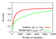
(a) Edge accuracy (C-P)

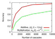
(b) Edge accuracy (HI)

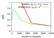
(c) MSE (C-P)

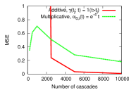
(d) MSE (HI)

Figure 1: Edge accuracy and MSE of our inference methods for additive and multiplicative propagation models against number of cascades. We used 1,024 node Core-Periphery (C-P) and Hierarchical (HI) Kronecker networks with an average of four edges per node and $T=4$.

5.1 Experiments on synthetic data

In this section, we compare the performance of our inference algorithms for additive and multiplicative models for different network structures, time shaping functions, baselines, and observation windows. We skip a comparison to other methods such as NetRate, KernelCascade, moNet or InfoPath since our model is able to mimic these methods by simply choosing the appropriate time shaping function $\gamma(\cdot;\cdot)$, Table 1. Rather, we focus on comparing multiplicative and additive models.

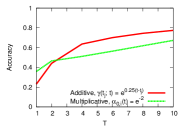
(a) Edge accuracy

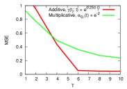
(b) MSE

Figure 2: Edge accuracy and MSE of our inference methods for additive and multiplicative propagation models against observation window. We used a 1,024 node Random Kronecker network with an average of 4 edges per node.

Experimental setup. First we generate realistic synthetic networks using the Kronecker graph model (Leskovec et al., 2010), and set the edge hazard function parameters $\alpha_{j,i}$ randomly, drawn from a uniform distribution. We then simulate and record a set of cascades propagating over the network using the additive or the multiplicative model. For each cascade we pick the cascade initiator node uniformly at random and generate the infection times following a similar procedure as in Austin (2012): We draw a uniform random variable per node, and then use inverse transform sampling (Devroye, 1986) to generate piecewise likelihoods of node infections. Note that every time a parent of node $i$ gets infected, we need to consider a new interval in the piecewise likelihood of infection of node $i$.

Performance vs. number of cascades. We evaluate our inference methods by computing two different measures: edge accuracy and mean squared error (MSE). Edge accuracy quantifies the fraction of edges the method was able to infer correctly: $1-\frac{\sum_{i,j}|I(\alpha^{*}_{i,j})-I(\hat{\alpha}_{i,j})|}{\sum_{i,j}I(\alpha^{*}_{i,j})+\sum_{i,j}I(\hat{\alpha}_{i,j})}$, where $I(\alpha)=1$ if $\alpha>0$ and $I(\alpha)=0$ otherwise. The MSE quantifies the error in the estimates of parameters $\alpha$: $E\big{[}(\alpha^{*}-\hat{\alpha})^{2}\big{]}$, where $\alpha^{*}$ is the true parameter of the model and $\hat{\alpha}$ is the estimated parameter.

Figure 1 shows the edge accuracy and the MSE against cascade size for two types of Kronecker networks: hierarchical and core-periphery, using different additive and multiplicative propagation models. Comparing additive and multiplicative models we find that in order to infer the networks to same accuracy the multiplicative model requires more data. This means it is more difficult to discover the network and fit the parameters for the multiplicative model than for the additive model. Moreover, estimating the value of the model parameters is considerably harder than simply discovering edges and therefore more cascades are needed for accurate estimates.

Performance vs. observation window length. Lengthening the observation window increases the number of observed infections and results in a more representative sample of the underlying dynamics. Therefore, it should intuitively result in more accurate estimates for both the additive and multiplicative models. Figure 2 shows performance against different observation window lengths for a random network (Erdős & Rényi, 1960), using additive and multiplicative models over 1,000 cascades. The experimental results support the above intuition. However, given a sufficiently large observation window, increasing further the length of the window does not increase performance significantly, as observed in case of the additive model with exponential time shaping function.

Topic or news event $(\bf{Q})$	# sites	# memes
Arab Spring	950	17,975
Bailout	1,127	36,863
Fukushima	1,244	24,888
Gaddafi	1,068	38,166
Kate Middleton	1,292	15,112

Table 2: Topic and news event statistics.

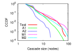
(a) CS: Arab Spring

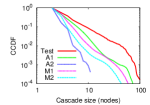
(b) CS: Bailout

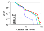
(c) CS: Fukushima

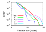
(d) CS: Gaddafi

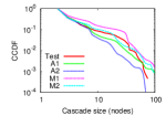
(e) CS: K. Middleton

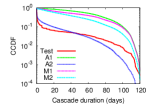
(f) CD: Arab Spring

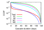
(g) CD: Bailout

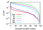
(h) CD: Fukushima

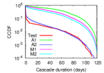
(i) CD: Gaddafi

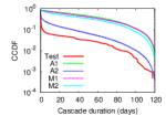
(j) CD: K. Middleton

Figure 3: Cascade size (CS) and cascade duration (CD) distributions for test sets on several topics. We compare the cascade test set (Test) against synthetic cascade sets, generated using two additive models, one (A1) with $\gamma(t_{j};t_{i})=I(t_{i}>t_{j})$ and other (A2) with $\gamma(t_{j};t_{i})=1/(t_{i}-t_{j})$, and two multiplicative models, one (M1) with $\alpha_{0,i}(t_{i})=e^{b}I(t_{i}>t_{j})$ and another (M2) with $\alpha_{0,i}(t_{i})=e^{b}/t_{i}$, where we set $b=-3$.

5.2 Experiments on real data

Experimental setup. We trace the flow of information using memes (Leskovec et al., 2009). Memes are short textual phrases (like, “lipstick on a pig”) that travel through a set of blogs and mainstream media websites. We consider each meme $m$ as a separate information cascade $c_{m}$. Since all documents which contain memes are time-stamped, a cascade $c_{m}$ is simply a record of times when sites first mentioned meme $m$. We use more than 10 million distinct memes from 3.3 million websites over a period of 4 months, from May 2011 till August 2011.

Our aim is to consider sites that actively spread memes over the Web, so we select the top 5,000 sites in terms of the number of memes they mentioned. Moreover, we are interested in inferring propagation models related to particular topics or events. Therefore, we consider we are also given a keyword query $Q$ related to the event/topic of interest. When we infer the parameters of the additive or multiplicative models for a given query $Q$, we only consider documents (and the memes they mention) that include keywords in $Q$. Table 2 summarizes the number of sites and meme cascades for several topics and real world events.

Unfortunately, true models (or ground truth) are unknown on real data. Previous network inference algorithms (Gomez-Rodriguez et al., 2010, 2011, 2013; Du et al., 2012) have been validated using explicit hyperlink cascades. However, the use of hyperlinks to refer to the source of information is relatively rare (especially in mainstream media) (Gomez-Rodriguez et al., 2010) and hyperlinks only allow us to test for nodes which increase the instantaneous risk of infection of other nodes, as in the additive risk model, but not for nodes which either increase or decrease it. To overcome this, we instead evaluate the predictive power of our models. For each query $Q$ we create a training and a test set of cascades. The training (test) set contains 80% (20%) of the recorded cascades for the event/topic of interest; both sets are disjoint and created at random. We use the training set to fit the parameters of our additive and multiplicative models and the test set to evaluate the models.

Cascade size prediction. For each event/topic of interest, we evaluate the predictive power of both models, learned using the training set, by comparing the cascade size distribution of the test set against a synthetically generated cascade set using the trained models. We build the synthetically generated cascade set by simulating a set of cascades starting from the true source nodes of the cascades in the test set using the model learned from the training set and an observation window equal to the one of the test set. Figures 3(a-e) show the distribution of cascade sizes for the test sets and for the synthetically generated cascade sets using two different additive models and two multiplicative models. None of the models is a clear winner in terms of similarity with the test sets, but the additive model with inverse linear time shaping function (A2) tends to underestimate the cascade size. Surprisingly, the cascade size distributions in the synthetically generated cascade sets are very similar to the empirical distributions, specially up to 10 infected nodes per cascade.

Cascade duration prediction. Next we further evaluate the predictive power of both models, learned using the training sets, by comparing the cascade duration distribution of the test sets against synthetically generated cascade sets using the trained models. Figures 3(f-j) show the distribution of the cascade duration of the test sets and the synthetically generated cascade sets using the same additive and multiplicative models. In this case, the performance of the models differs more dramatically. The additive model with inverse linear time shaping function gets the closest to the empirical distribution of the test set at the cost of underestimating the cascade size.

6 Conclusion

Our work here contributes towards a general mathematical theory of information propagation over networks while also providing flexible methods. Moreover, there are also many venues for future work. In the additive model, external influences that are endogenous to the network  (Myers et al., 2012) could be considered by including an extra additive term $\alpha_{i0}(t)$. In the multiplicative model, one could consider nonparametric baselines $\alpha_{i,0}(t)$ by fitting the model using partial likelihood. Both models could be extended to include other types of covariates $\mathbf{s}(t)$ and also to consider time varying parameters $\alpha_{ji}(t)$ in order to infer dynamic networks (Gomez-Rodriguez et al., 2013). Finally, developing goodness of fit tests would be useful to choose among models in a more principled manner.

References

- Aalen et al. (2008) Aalen, O.O., Borgan, Ø., and Gjessing, H.K. Survival and event history analysis: a process point of view. Springer Verlag, 2008.
- Austin (2012) Austin, P.C. Generating survival times to simulate cox proportional hazards models with time-varying covariates. Statistics in Medicine, 2012.
- Bailey (1975) Bailey, N. T. J. The Mathematical Theory of Infectious Diseases and its Applications. Hafner Press, 2nd edition, 1975.
- Boyd & Vandenberghe (2004) Boyd, S.P. and Vandenberghe, L. Convex optimization. Cambridge University Press, 2004.
- Devroye (1986) Devroye, L. Non-uniform random variate generation, volume 4. Springer-Verlag New York, 1986.
- Du et al. (2012) Du, N., Song, L., Smola, A., and Yuan, M. Learning networks of heterogeneous influence. In NIPS ’12: Neural Information Processing Systems, 2012.
- Erdős & Rényi (1960) Erdős, P. and Rényi, A. On the evolution of random graphs. Publication of the Mathematical Institute of the Hungarian Academy of Science, 5:17–67, 1960.
- Gomez-Rodriguez & Schölkopf (2012) Gomez-Rodriguez, M. and Schölkopf, B. Submodular Inference of Diffusion Networks from Multiple Trees. In ICML ’12: Proceedings of the 29th International Conference on Machine Learning, 2012.
- Gomez-Rodriguez et al. (2010) Gomez-Rodriguez, M., Leskovec, J., and Krause, A. Inferring Networks of Diffusion and Influence. In KDD ’10: Proceedings of the 16th ACM SIGKDD International Conference on Knowledge Discovery and Data Mining, 2010.
- Gomez-Rodriguez et al. (2011) Gomez-Rodriguez, M., Balduzzi, D., and Schölkopf, B. Uncovering the Temporal Dynamics of Diffusion Networks. In ICML ’11: Proceedings of the 28th International Conference on Machine Learning, 2011.
- Gomez-Rodriguez et al. (2013) Gomez-Rodriguez, M., Leskovec, J., and Schölkopf, B. Structure and Dynamics of Information Pathways in On-line Media. In WSDM ’13: Proceedings of the 6th ACM International Conference on Web Search and Data Mining, 2013.
- Kempe et al. (2003) Kempe, D., Kleinberg, J. M., and Tardos, É. Maximizing the spread of influence through a social network. In KDD ’03: Proceedings of the 9th ACM SIGKDD International Conference on Knowledge Discovery and Data Mining, 2003.
- Leskovec et al. (2006) Leskovec, J., Adamic, L. A., and Huberman, B. A. The dynamics of viral marketing. In EC’ 06: Proceedings of the eigth International Conference on Electronic Commerce, 2006.
- Leskovec et al. (2009) Leskovec, J., Backstrom, L., and Kleinberg, J. Meme-tracking and the dynamics of the news cycle. In KDD ’09: Proceedings of the 15th ACM SIGKDD International Conference on Knowledge Discovery and Data Mining, 2009.
- Leskovec et al. (2010) Leskovec, J., Chakrabarti, D., Kleinberg, J., Faloutsos, C., and Ghahramani, Z. Kronecker graphs: An approach to modeling networks. Journal of Machine Learning Research, 11:985–1042, 2010.
- Liben-Nowell & Kleinberg (2008) Liben-Nowell, David and Kleinberg, Jon. Tracing the flow of information on a global scale using Internet chain-letter data. Proceedings of the National Academy of Sciences, 105(12):4633–4638, 2008.
- Myers & Leskovec (2010) Myers, S. and Leskovec, J. On the Convexity of Latent Social Network Inference. In NIPS ’10: Neural Information Processing Systems, 2010.
- Myers et al. (2012) Myers, S., Leskovec, J., and Zhu, C. Information Diffusion and External Influence in Networks. In KDD ’12: Proceedings of the 18th ACM SIGKDD International Conference on Knowledge Discovery and Data Mining, 2012.
- Netrapalli & Sanghavi (2012) Netrapalli, P. and Sanghavi, S. Finding the graph of epidemic cascades. In ACM SIGMETRICS/Performance ’12: Proceedings of the ACM SIGMETRICS and Performance Conference, 2012.
- Rogers (1995) Rogers, E. M. Diffusion of Innovations. Free Press, New York, fourth edition, 1995.
- Saito et al. (2009) Saito, K., Kimura, M., Ohara, K., and Motoda, H. Learning continuous-time information diffusion model for social behavioral data analysis. Advances in Machine Learning, pp. 322–337, 2009.
- Snowsill et al. (2011) Snowsill, T.M., Fyson, N., De Bie, T., and Cristianini, N. Refining causality: who copied from whom? In KDD ’11: Proceedings of the 17th ACM SIGKDD International Conference on Knowledge Discovery and Data Mining, 2011.
- Wang et al. (2012) Wang, L., Ermon, S., and Hopcroft, J. Feature-enhanced probabilistic models for diffusion network inference. In ECML PKDD ’12: Proceedings of the European Conference on Machine Learning and Principles and Practice of Knowledge Discovery in Databases, 2012.