Explaining observations of rapidly rotating neutron stars in LMXBs

Abstract

In a previous paper [M. E. Gusakov, A. I. Chugunov, and E. M. Kantor, Phys. Rev. Lett. 112, 151101 (2014)], we introduced a new scenario that explains the existence of rapidly rotating warm neutron stars (NSs) observed in low-mass X-ray binaries (LMXBs). Here it is described in more detail. The scenario takes into account the interaction between superfluid inertial modes and the normal (quadrupole) $m=2$ $r$-mode, which can be driven unstable by Chandrasekhar-Friedman-Schutz (CFS) mechanism. This interaction can only occur at some fixed “resonance” stellar temperatures; it leads to formation of the “stability peaks” which stabilize a star in the vicinity of these temperatures. We demonstrate that a NS in LMXB spends a substantial fraction of time on the stability peak, that is, in the region of stellar temperatures and spin frequencies, that has been previously thought to be CFS unstable with respect to excitation of $r$-modes. We also find that the spin frequencies of NSs are limited by the CFS instability of normal (octupole) $m=3$ $r$-mode rather than by $m=2$ $r$-mode. This result agrees with the predicted value of the cutoff spin frequency $\sim 730$ Hz in the spin distribution of accreting millisecond X-ray pulsars. In addition, we analyze evolution of a NS after the end of the accretion phase and demonstrate that millisecond pulsars can be born in LMXBs within our scenario. Besides millisecond pulsars, our scenario also predicts a new class of LMXB descendants—hot and rapidly rotating nonaccreting NSs (“hot widows”/HOFNARs). Further comparison of the proposed theory with observations of rotating NSs can impose new important constraints on the properties of superdense matter.

I Introduction

Neutron stars (NSs) are the compact rotating objects with a mass $M\sim M_{\odot}$ and radius $R\sim 10$ km (e.g., Ref. Haensel et al. (2007)). Rotation leads to the appearance of the so-called inertial oscillation modes in NSs, whose restoring force is the Coriolis force Unno et al. (1989). A particular, but the most interesting class of inertial modes is $r$-modes for which (unlike the other inertial modes) the dominant oscillations are of toroidal type Andersson and Kokkotas (2001). The remarkable property of $r$-modes is that, neglecting dissipation, they are subject to a gravitationally driven Chandrasekhar-Friedman-Schutz (CFS) instability at arbitrary spin frequency $\nu$ of a NS Andersson (1998); Friedman and Morsink (1998). An account for dissipative effects stabilizes the NS to some extent resulting in the appearance of the “stability region” in the $\nu-T^{\infty}$ plane, where $T^{\infty}$ is the redshifted internal stellar temperature. A typical stability region is shaded in grey in Fig. 2 (see Sec. III.2); $r$-modes cannot be spontaneously excited inside this region.

In some cases observations of rapidly rotating NSs in low-mass X-ray binaries (LMXBs) allow one to measure $\nu$ (e.g., Refs. Patruno (2010); Patruno and Watts (2012)) and estimate $T^{\infty}$ (e.g., Refs. Ho et al. (2011); Haskell et al. (2012); Mahmoodifar and Strohmayer (2013) and Table 1). It turns out that many of the rapidly rotating warm sources fall well outside the stability region, if it is plotted under realistic assumptions about the properties of superdense matter Ho et al. (2011); Haskell et al. (2012). In fact, calculations show that NSs in LMXBs can indeed leave the stability region for a while, but the probability to observe them there is negligibly small in most cases (see, e.g., Refs. Levin (1999); Heyl (2002) and Sec. III). Thus, we face a paradox which is usually being explained following one of the two approaches.

In the first approach one tries, making some (rather artificial) assumptions, to enhance damping of $r$-mode oscillations due to various dissipative mechanisms. The aim is to enlarge the stability region so that it would contain all the observed sources (see, e.g., Andersson and Kokkotas (2001); Haskell et al. (2012)).

The second approach assumes that some fraction of NSs lies outside the stability region, but their spin frequency $\nu$ and temperature $T^{\infty}$ are determined by two conditions that should be satisfied simultaneously: ($i$) $r$-mode oscillations in these NSs should reach saturation because of nonlinear interaction with other inertial modes (see, e.g., Ho et al. (2011); Mahmoodifar and Strohmayer (2013) and Sec. III.2) and ($ii$) all the heat released due to dissipation of the “saturated” $r$-modes should be radiated away by the neutrino emission. Unfortunately, these conditions lead to unrealistically small values of the saturation amplitude $\alpha_{\rm sat}\sim 10^{-9}$–$10^{-6}$, specific to each source Ho et al. (2011); Mahmoodifar and Strohmayer (2013). Such small $\alpha_{\rm sat}$ seem to contradict the results of Refs. Bondarescu et al. (2007, 2009) (see also footnote 13 below).

Thus, one can conclude that the existence of rapidly rotating warm NSs remains an open problem Andersson et al. (2013). A possible solution to this problem was suggested in our recent paper Gusakov et al. (2014) and is discussed in more detail here. Our key idea consists in that to study evolution of NSs in LMXBs one has to correctly take into account the resonance interaction between the normal oscillation $m=2$ $r$-mode and superfluid inertial modes, which occurs at some fixed values of $T^{\infty}$ (see Sec. IV). Such resonance interaction has been completely ignored in the literature so far. However, as we will argue below, it should take place and can dramatically affect the evolution of rapidly rotating NSs.

First of all, this interaction modifies the stability region (see Sec. V) and allows us to suggest an evolution scenario (Sec. VI), that explains all the sources in LMXBs within the standard, minimal assumptions about the composition and properties of superdense matter. Moreover, as directly follows from our scenario, the NS spin frequencies $\nu$ appear to be bounded by the onset of the octupole $m=3$ oscillation $r$-mode instability, which corresponds to $\nu\sim 600$–$700$ Hz at $T^{\infty}\sim 10^{8}$ K (see Fig. 5). The existence of an upper bound for $\nu$ can explain the sharp cutoff of the distribution function for accreting X-ray pulsars at a frequency $\nu\gtrsim 730$ Hz Chakrabarty et al. (2003); Chakrabarty (2008). If correct, this result presents a strong argument in favor of the idea of Refs. Bildsten (1998); Andersson et al. (1999) that the NS spin frequency $\nu$ is limited by the $r$-mode instability. Note, however, that in our scenario $\nu$ is limited by the octupole $m=3$ $r$-mode rather than by quadrupole $m=2$ $r$-mode, as it is supposed in Refs. Bildsten (1998); Andersson et al. (1999).

The paper is organized as follows. In Sec. II we discuss the adopted NS model and write out general equations governing the thermorotational evolution of a NS in LMXB with allowance for the excitation of normal $r$-modes. In Sec. III we present the summary of observations of quiescent temperatures and spin frequencies for NSs in LMXBs, and demonstrate the problem with their explanation within the scenarios available in the literature. In Sec. IV we describe and justify our model of resonance interaction between the normal and superfluid oscillation modes. In Sec. V we determine the stability region taking into account the resonance interaction of the normal $m=2$ $r$-mode and one of the superfluid inertial modes; we also generalize the equations describing the NS dynamics to the case when a few oscillation modes are simultaneously excited in a star. These results are applied in Sec. VI to model the evolution of an accreting NS. Detailed analysis of the evolution tracks allow us to formulate an original scenario explaining all the existing data on the spin frequencies and temperatures of NSs in LMXBs. In Sec. VII we discuss the NS evolution after the end of the accretion phase. We argue that our scenario can explain observations of millisecond pulsars and also predicts the existence of a new possible class of hot, nonaccreting, and rapidly rotating NSs. In Sec. VIII we present the main conclusions.

II Physics input and general equations

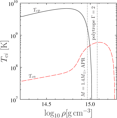
Figure 1: (color online) Critical temperatures of protons $T_{{\rm c}p}$ (solid line; black online) and neutrons $T_{{\rm c}n}$ (dashed line; red online) as functions of density $\rho$ in neutron star core. Vertical dotted lines indicate central densities of a star with the mass $M=1.4M_{\odot}$. The left line corresponds to the relativistic star with the Akmal-Pandharipande-Ravenhall (APR) EOS Akmal et al. (1998), the right line corresponds to the polytropic Newtonian star (polytropic exponent $\Gamma=2$) with the radius $R=10$ km.

All calculations in this paper are carried out for a canonical NS with the mass $M=1.4M_{\odot}$ and radius $R=10$ km, whose core is composed of neutrons ($n$), protons ($p$) and electrons ($e$). Following Refs. Owen et al. (1998); Lindblom et al. (1998); Ho and Lai (2000); Heyl (2002); Wagoner (2002) we, for simplicity, consider the polytropic equation of state (EOS) with polytropic index $n=1$ ($P\propto\rho^{\Gamma}$, where $\Gamma=1+1/n=2$; $P$ and $\rho$ are, respectively, the pressure and density of matter). We checked, that use of more realistic EOSs does not affect our main results (see also Ref. Andersson and Kokkotas (2001)).

According to numerous microscopic calculations, nucleons (neutrons and protons) in the internal layers of NSs are superfluid at temperatures $T\;\raise 1.29167pt\hbox{$<$\kern-7.5pt\raise-4.73611pt\hbox{$\sim$}}\;10^{8}$–$10^{10}$ K. Recent real-time observations of a cooling young NS in Cassiopeia A supernova remnant Heinke and Ho (2010) have presented strong evidence of this fact (but see a critique in Ref. Posset_etal13 ). They were explained Shternin et al. (2011); Page et al. (2011) within the so-called “minimal cooling scenario,” proposed in Refs. Gusakov et al. (2004); Page et al. (2004). In this paper we use the same models of neutron and proton superfluidity [that is, the same functions $T_{{\rm c}i}(\rho)$, where $T_{{\rm c}i}$ is the critical temperature for transition of a nucleon species $i=n$, $p$ to the superfluid state] as in Ref. Gusakov et al. (2004) (see Fig. 1); these models are analogous to those used in Ref. Shternin et al. (2011) to explain the NS cooling in Cassiopeia A supernova remnant. The superfluidity models adopted here are also capable of explaining all observations of cooling isolated NSs available to date Gusakov et al. (2004); Gusakov et al. (2005a).

To analyze oscillations of rotating stars it is convenient to separate the variable $\phi$ that describes the azimuthal angle in the plane perpendicular to the stellar rotation axis, and to present all perturbations as $\propto\exp(\imath m\phi)$, where $m$ is an integer. As it was shown in Refs. Andersson and Comer (2001); Lee and Yoshida (2003); Yoshida and Lee (2003a, b); Kantor and Gusakov (2013), inertial modes of two types exist in superfluid NSs for any $m$. In Ref. Yoshida and Lee (2003a) they were termed $i^{o}$- and $i^{s}$-modes. The modes of the first type, which we call “normal” ($i^{o}$-modes) describe comoving oscillations of superfluid and normal matter components and resemble, in many aspects, the corresponding modes of a normal (nonsuperfluid) star Gusakov and Kantor (2011); Gusakov et al. (2013); Kantor and Gusakov (2013); Gualtieri et al. (2014). The modes of the second type, which we call “superfluid” ($i^{s}$-modes) correspond to countermoving oscillations of superfluid and normal matter components and are absent in normal stars. As it was first demonstrated in Refs. Lee and Yoshida (2003); Yoshida and Lee (2003a), a gravitationally driven instability of $i^{s}$-modes is strongly suppressed, because their gravitational radiation is weak, while dissipation of these modes is dramatically enhanced due to the powerful mutual friction mechanism (see, e.g., Refs. Alpar et al. (1984); Andersson et al. (2006) and Sec. IV.1 for more details on the mutual friction force). Among $i^{o}$-modes we only consider the normal $r$-modes with $m=2$ and $m=3$, since they are the most unstable ones Owen et al. (1998); Andersson and Kokkotas (2001). Following Ref. Yoshida and Lee (2003a) we denote the normal $r$-modes as $r^{o}$-modes; in this section we analyze them in more detail.

In $r^{o}$-modes the oscillations are predominantly of toroidal type. In that case, to leading order in $\Omega$ (where $\Omega=2\pi\nu$ is the circular spin frequency), the Eulerian velocity perturbation $\delta\boldsymbol{v}$ can be presented as Provost et al. (1981)

$$\delta{\boldsymbol{v}}=\alpha\frac{\Omega Rr}{\sqrt{l(l+1)}}\left(\frac{r}{R}\right)^{l}{\boldsymbol{\nabla}}\times(r{\boldsymbol{\nabla}}Y_{lm})\mathrm{e}^{\imath\omega t},$$ (1)

where $Y_{lm}$ is the spherical harmonic with the multipolarity $l$ equal to $m$, $l=m$; $\alpha$ is the oscillation amplitude of the $r^{o}$-mode; $r$ is the radial coordinate. Finally, $\omega$ is the oscillation frequency in the inertial frame, given by (also to leading order in $\Omega$) Papaloizou and Pringle (1978)

$$\omega=-\frac{(l-1)(l+2)}{l+1}\,\Omega.$$ (2)

Below we make use of the quantity

$$\Omega_{0}\equiv\sqrt{\pi\,G\,\bar{\rho}}\approx 1.180\times 10^{4}\,\left(\frac{M}{1.4M_{\odot}}\right)^{1/2}\left(\frac{R}{10\ \mathrm{km}}\right)^{-3/2}\mathrm{s}^{-1},$$ (3)

where $G$ is the gravitation constant and $\bar{\rho}=3M/(4\pi R^{3})$ is the mean stellar density. For a canonical NS $\bar{\rho}\approx 6.646\times 10^{14}$ g cm^-3.

To describe the evolution of a NS allowing for the $r^{o}$-mode instability, we follow the phenomenological approach suggested by Owen et al. Owen et al. (1998) and further refined in Refs. Ho and Lai (2000) and Alford and Schwenzer (2014). We mostly employ the notation of Ref. Ho and Lai (2000). The evolution is given by the following equations:

($i$) An equation governing the variation of canonical angular momentum $J_{\rm c}$ of the $r^{o}$-mode due to radiation of gravitational waves and various dissipative effects,

$$\frac{dJ_{\rm c}}{dt}=-2\,J_{\rm c}\,\left(\frac{1}{\tau_{\rm GR}}+\frac{1}{\tau_{\rm Diss}}\right).$$ (4)

Here Friedman and Schutz (1978a); Owen et al. (1998)

$$J_{\rm c}=-\frac{l}{2(\omega+l\Omega)}\int\rho\,\delta{\boldsymbol{v}}\,\delta{\boldsymbol{v}}^{\ast}d^{3}r=-\frac{\alpha^{2}\,l(l+1)}{4}\Omega R^{-2l+2}\int_{0}^{R}\rho r^{2l+2}dr,$$ (5)

where we apply Eqs. (1) and (2) in the second equality. An integral in the right-hand side of Eq. (5) can be easily calculated if one specifies the density profile $\rho(r)$. Obviously, the integral can generally be written in the form $\widetilde{J}\,M\,R^{2l}$, where $\widetilde{J}$ is some numerical coefficient that depends on $\rho(r/R)$. Using this expression, $J_{\rm c}$ can be presented as

$$J_{\rm c}=-\frac{l(l+1)}{4}\,\widetilde{J}\,\,M\,R^{2}\,\Omega\,\alpha^{2}.$$ (6)

For the simple polytropic model with $\Gamma=2$ and a given stellar mass $M$ and radius $R$, one has

$$\rho(r)=\frac{M}{4\,r\,R^{2}}\,\sin\left(\frac{\pi r}{R}\right),$$ (7)

which leads to $\widetilde{J}\approx 1.6353\times 10^{-2}$ for $l=m=2$ and $\widetilde{J}\approx 9.9887\times 10^{-3}$ for the $l=m=3$ $r^{o}$-mode.

An intensity of gravitational radiation is determined by the mass current multipole; using Eq. (1) one can calculate the corresponding gravitational radiation time scale $\tau_{\rm GR}$ Lindblom et al. (1998),

$$\frac{1}{\tau_{\rm GR}}=-\frac{32\,\pi\,G\,\Omega^{2l+2}}{c^{2l+3}}\,\frac{(l-1)^{2l}}{[(2l+1)!!]^{2}}\,\left(\frac{l+2}{l+1}\right)^{2l+2}\,\int_{0}^{R}\rho\,r^{2l+2}dr,$$ (8)

where $c$ is the speed of light. For the density profile (7) this expression can be rewritten as Andersson and Kokkotas (2001)

$$\tau_{\rm GR}=-\tau_{\rm GR\,0}\left(\frac{M}{1.4M_{\odot}}\right)^{-1}\,\left(\frac{R}{10\,\mathrm{km}}\right)^{-2l}\,\left(\frac{\nu}{1\mathrm{kHz}}\right)^{-2l-2},$$ (9)

where $\tau_{{\rm GR}\,0}\approx 46.4$ s and $1250$ s for $l=m=2$ and $l=m=3$ $r^{o}$-modes, respectively.

Further, $1/\tau_{\rm Diss}$ in Eq. (4) is generally presented in the form,

$$\frac{1}{\tau_{\rm Diss}}=\sum_{i}\frac{1}{\tau_{i}},$$ (10)

where the summation is assumed over all possible processes resulting in dissipation of energy and angular momentum of $r^{o}$-modes (the shear and bulk viscosities, Ekman layer dissipation, mutual friction etc. Andersson and Kokkotas (2001)). In this paper, we neglect the bulk viscosity, because it is small for the range of stellar temperatures $T<5\times 10^{8}$ K we are interested in (see, e.g., Haensel et al. (2001); Gusakov (2007); Kantor and Gusakov (2011); Gusakov et al. (2013)). One can also freely ignore the effects of mutual friction when considering $r^{o}$-modes Lindblom and Mendell (2000); Lee and Yoshida (2003); Haskell et al. (2009). On the opposite, dissipation in the Ekman layer can be a very efficient mechanism, though the corresponding damping time $\tau_{\rm Ek}$ is very sensitive to the chosen model of interaction between the “solid” crust and liquid core of a NS Levin and Ushomirsky (2001); Yoshida and Lee (2001); Andersson and Kokkotas (2001); Rieutord (2001a, b); Glampedakis and Andersson (2006a); Kinney and Mendell (2003); Mendell (2001). Actually, in the vicinity of the crust-core interface the crust is neither solid nor liquid, being some intermediate structure, which is called mantle. Thus, dissipation in the transition Ekman layer can be substantially lower than it is often assumed.

Bearing this in mind, we consider dissipation due to the shear viscosity as our minimal model for the dissipation of $r^{o}$-modes. The corresponding time scale $\tau_{\rm S}$ can be calculated from the formula Lindblom et al. (1998)

$$\frac{1}{\tau_{\rm S}}=(l-1)(2l+1)\,\int_{0}^{R}\eta\,r^{2l}\,dr\,\,\left(\int_{0}^{R}\rho\,r^{2l+2}dr\right)^{-1},$$ (11)

that was obtained using velocity field (1). Here $\eta$ is the shear viscosity coefficient. Estimates show that the proton shear viscosity is small in comparison to the electron one $\eta_{e}$ Shternin and Yakovlev (2008), while the neutron shear viscosity is poorly known even for nonsuperfluid NS matter (its value differs for different authors by a factor of 5–10 and can be either greater Benhar and Valli (2007); Zhang et al. (2010) or smaller Shternin and Yakovlev (2008); Shternin et al. (2013) than $\eta_{e}$). In view of these facts, for $\eta$ in this paper we take the electron shear viscosity $\eta_{e}$ from Ref. Shternin and Yakovlev (2008). Notice that $\eta_{e}$ can vary several-fold depending on a chosen EOS (or, more precisely, depending on a proton fraction predicted by an EOS; see, e.g., figure 1 in Ref. Shternin and Yakovlev (2008)). Another important ingredient, affecting $\eta_{e}$ Shternin and Yakovlev (2008), is still poorly known model of proton superfluidity [the profile $T_{{\rm c}p}(\rho)$].

The uncertainties, described above, and possible contribution of the Ekman layer into dissipation, can effectively increase $\eta$ by a factor of few. For octupole ($l=m=3$) $r^{o}$-mode the situation is even more uncertain, because this mode becomes unstable (and thus important for the NS evolution; see Sec. V) at rather high values of $\Omega$. This means that the approximation of slowly rotating NSs, assumed in derivation of Eqs. (8) and (11), can lead to larger errors for the octupole $r^{o}$-mode Jones et al. (2002); Karino et al. (2000). Taking this into account, when modeling the octupole $r^{o}$-mode (but not the quadrupole $r^{o}$-mode!), for $\eta$ we take (somewhat arbitrary) $\eta_{e}$ from Ref. Shternin and Yakovlev (2008), multiplied by a factor of $5$; that is, we set $\eta=5\eta_{e}$.

Using the results of Ref. Shternin and Yakovlev (2008), we approximate the electron shear viscosity $\eta_{e}$ by the following fitting formula,

$$\eta_{e}=6\times 10^{18}\,\left(\frac{\rho}{10^{15}\ \mathrm{g}\,\mathrm{cm}^{-3}}\right)^{2}\left(\frac{T}{10^{9}\,{\rm K}}\right)^{-2}\left(\frac{T_{{\rm c}p}}{2\times 10^{9}\,{\rm K}}\right)^{1/3}\quad\frac{{\rm g}}{{\rm cm}\,{\rm s}},$$ (12)

which particularly well describes $\eta_{e}$ for the APR EOS Akmal et al. (1998) (more precisely, for the parametrization Heiselberg and Hjorth-Jensen (1999) of the APR EOS). Notice that this formula is valid only if protons are superfluid and $T\;\raise 1.29167pt\hbox{$<$\kern-7.5pt\raise-4.73611pt\hbox{$\sim$}}\;\,0.2\,T_{{\rm c}p}$. Notice also that, without the last multiplier, the formula (12) coincides with the well-known and widely used fit Cutler and Lindblom (1987) of old calculations of Flowers and Itoh Flowers and Itoh (1979). This is an accidental and surprising coincidence, because the physics input used in Refs. Shternin and Yakovlev (2008) and Flowers and Itoh (1979) is essentially different (in particular, unlike Ref. Shternin and Yakovlev (2008), $\eta_{e}$ from the paper by Flowers and Itoh was derived assuming no proton superfluidity and, what is more important, accounting incorrectly for the effects of transverse plasma screening on the processes of electron-electron scattering). In addition, the fitting formula of Ref. Cutler and Lindblom (1987) was obtained for an absolutely different EOS.

For our model of the proton superfluidity the last multiplier in Eq. (12) is of the order of unity in the greatest portion of the star, $[T_{{\rm c}p}(\rho)/(2\times 10^{9}\,{\rm K})]^{1/3}\sim 1$. In view of the uncertainties in the value of $\eta$, we ignore this multiplier in what follows. Using Eq. (12) and integrating (11) over $r$, we obtain

$$\tau_{\rm S}=\tau_{{\rm S}\,0}\left(\frac{R}{10\,\mathrm{km}}\right)^{5}\left(\frac{M}{1.4M_{\odot}}\right)^{-1}\,\left(T^{\infty}_{8}\right)^{2},$$ (13)

where $T^{\infty}_{8}\equiv T^{\infty}/(10^{8}\,{\rm K})$; $\tau_{{\rm S}\,0}\approx 2.2\times 10^{5}$ s for the $l=m=2$ $r^{o}$-mode and $\tau_{{\rm S}\,0}\approx 2.4\times 10^{4}$ s for the $l=m=3$ $r^{o}$-mode (we remind the reader that in the latter case we take $\eta=5\eta_{e}$). In Eq. (13), instead of $T$, we introduced the redshifted internal temperature $T^{\infty}\equiv T\,{\rm e}^{\nu(r)/2}$, where $\nu(r)$ is the corresponding metric coefficient Chandrasekhar (1964). Let us remind the reader that in the nonrelativistic approximation which has been used in derivation of this equation, $T=T^{\infty}$, so that such replacement is justified. Moreover, the temperature $T^{\infty}$, which is constant over the star, is a more appropriate parameter than $T$ for the description of NS thermal evolution [see Eq. (16) below] and, especially, for the analysis of observational data (Sec. III.1).

($ii$) An equation describing the change in the total angular momentum $J_{\rm c}+I\Omega$ of a NS,

$$\frac{d(J_{\rm c}+I\Omega)}{dt}=-\frac{2}{\tau_{\rm GR}}\,J_{\rm c}+\dot{J}_{\mathrm{acc}},$$ (14)

due to gravitational wave radiation (the first term) and accretion from the low-mass companion (the second term $\dot{J}_{\mathrm{acc}}$). For simplicity, we ignore possible magnetodipole torque in this paper (but see Sec. VI). In Eq. (14) $I=\widetilde{I}\,MR^{2}$ is the stellar moment of inertia; for a polytropic EOS ($\Gamma=2$) $\widetilde{I}\approx 0.261$. There is a number of accretion models, leading to somewhat different estimates for $\dot{J}_{\mathrm{acc}}$ (e.g., Ghosh and Lamb (1979); Rappaport et al. (2004); Kluźniak and Rappaport (2007)); however, they do not agree well with observations (see, e.g., Patruno and Watts (2012); Andersson et al. (2014)). Thus, for definiteness, we make use of the simplest estimate,

$$\dot{J}_{\mathrm{acc}}=p\,\dot{M}\,\sqrt{GMR},$$ (15)

which is traditionally applied in modeling the NS evolution in binary systems. Here $\dot{M}$ is the mass of accreted matter per unit time; $p$ depends on the physics of accretion (i.e., on the NS magnetic field, spin frequency $\Omega$, accretion rate etc.; see, e.g., Ref. Rappaport et al. (2004)). For simplicity, we take $p=1$ (e.g., Ref. Levin (1999)). Below we analyze the large time-scale evolution of NSs; hence, we assume that the quantities $\dot{J}_{\mathrm{acc}}$ and $\dot{M}$ are averaged over the active and quiescent phases of accretion. Since $\dot{J}_{\mathrm{acc}}\propto\dot{M}$ in Eq. (15), one can use that expression for the averaged values as well. In what follows we set $p=1$ and $\dot{M}=3.0\times 10^{-10}\,M_{\odot}$ yr^-1. The chosen value of $\dot{M}$ is close to the estimates of the accretion rates for the sources SAX J1750.8-2900 and 4U 1608-522 (see below).

($iii$) An equation describing the thermal evolution of an oscillating star,

$$C_{\rm tot}\frac{dT^{\infty}}{dt}=W_{\rm Diss}-L_{\rm cool}+K_{\rm n}\dot{M}c^{2},$$ (16)

where $W_{\rm Diss}$ is the energy dissipated per unit time due to the $r^{o}$-mode damping. It is presented as (e.g., Ref. Levin (1999))

$$W_{\rm Diss}=\frac{2E_{\rm c}}{\tau_{\rm Diss}}=\frac{\widetilde{J}MR^{2}\Omega^{2}\alpha^{2}}{\tau_{\rm Diss}},$$ (17)

where $E_{\rm c}$ is the canonical energy of the $r^{o}$-mode (with arbitrary $m$) in a reference frame, rotating with the star. As it was shown in Refs. Friedman and Schutz (1978b, a), $E_{\rm c}$ is related to the canonical angular momentum $J_{c}$ [see Eq. (6)] by

$$E_{\rm c}=-\frac{(\omega+m\Omega)}{m}\,J_{\rm c}.$$ (18)

This relation is valid for any inertial modes (not only for $r^{o}$-modes). Further, $C_{\rm tot}(T^{\infty})$ in Eq. (16) is the total heat capacity of a NS; $L_{\rm cool}(T^{\infty})$ is its luminosity, that is, the energy carried away from the star per unit time in the form of neutrino and electromagnetic radiation from its surface. Since oscillation amplitudes of $r^{o}$-modes, analyzed in this paper, are small ($\alpha\leq 10^{-4}$, see below), $L_{\rm cool}$ is given by the same equation as for a nonoscillating star Gusakov et al. (2005b). To determine the quantities $C_{\rm tot}$ and $L_{\rm cool}$ as accurately as we can, we calculate them with the relativistic cooling code, described in detail in Refs. Gusakov et al. (2004); Gusakov et al. (2005a); Yakovlev and Pethick (2004) (we used essentially the same microphysics input as that employed in Ref. Gusakov et al. (2004)). In particular, we used the parametrization Heiselberg and Hjorth-Jensen (1999) of the APR EOS Akmal et al. (1998) and considered a star with the mass $M=1.4M_{\odot}$. Although this approach is somewhat inconsistent (other equations neglect relativistic effects and employ the polytropic EOS), it allows us to use the realistic values for $C_{\rm tot}$ and $L_{\rm cool}$ in our simplified model. The calculations of $C_{\rm tot}$ and $L_{\rm cool}$ have been roughly approximated as functions of internal (redshifted) stellar temperature $T^{\infty}$ and are presented in Appendix A. Since the photon luminosity is not important in the temperature range of interest to us ($T^{\infty}>10^{8}$ K), we fit only the neutrino luminosity in Appendix A. Note that for lower $T^{\infty}$ the photon luminosity rapidly becomes the main cooling agent and hence cannot be ignored Yakovlev and Pethick (2004). We have checked, that the results for $r^{o}$-mode evolution obtained using the fitting formulas from Appendix A, practically do not differ from those obtained using the exact values for $C_{\rm tot}$ and $L_{\rm cool}$.

Finally, the last term in Eq. (16) describes the stellar heating due to accretion (deep crustal heating, see, e.g., Ref. Brown et al. (1998)). Under the pressure of accreted material, the matter in the stellar envelope compresses and eventually undergoes a set of exothermal nuclear transformations (pycnonuclear reactions and reactions of beta-capture, accompanied by the neutron emission). The heat released in these reactions is mostly accumulated by the core due to high thermal conductivity of the internal layers of NSs. The parameter $K_{\rm n}$ characterizes the efficiency of this heating; following Refs. Brown (2000); Bondarescu et al. (2007) we adopt $K_{\rm n}=10^{-3}$ as a fiducial value. For a chosen NS model, the heating (in the absence of a $r^{o}$-mode) is completely compensated by the cooling ($L_{\rm cool}=K_{\rm n}\dot{M}c^{2}$) at $T_{\rm eq}^{\infty}\approx 1.078\times 10^{8}$ K.

Equations (4), (14), and (16) fully describe the evolution of nonsaturated $r^{o}$-modes. Using Eqs. (4) and (14) one can express the quantities $d\alpha/dt$ and $d\Omega/dt$,

$$\frac{d\alpha}{dt} = -\alpha\left(\frac{1}{\tau_{\rm GR}}+\frac{1}{\tau_{\rm Diss}}\right),$$ (19)

$$\frac{d\Omega}{dt} = -\frac{2\,Q\,\alpha^{2}\,\Omega}{\tau_{\rm Diss}}+\dot{\Omega}_{\rm acc},$$ (20)

where

$$\dot{\Omega}_{\rm acc} \equiv \dot{J}_{\mathrm{acc}}/I=p\,\dot{M}\,\frac{\sqrt{GMR}}{I}$$ (21)

$$\approx 3.73\times 10^{-6}\,\,p\,\,\dot{M}_{-10}\,\,\widetilde{I}_{0.261}^{-1}\,\,\left(\frac{M}{1.4M_{\odot}}\right)^{-1/2}\,\left(\frac{R}{10\,{\rm km}}\right)^{-3/2}\,{\rm s^{-1}\,yr^{-1}},$$

$$Q \equiv \frac{l(l+1)\widetilde{J}}{4\widetilde{I}},$$ (22)

and $\dot{M}_{-10}=\dot{M}/(10^{-10}\,M_{\odot}\,{\rm yr}^{-1})$, $\widetilde{I}_{0.261}=\widetilde{I}/0.261$. In deriving Eq. (19) we neglected the term $\propto\alpha^{3}$, assuming that $\alpha\ll 1$. In addition, because $\dot{\Omega}_{\rm acc}/\Omega\ll 1/\tau_{\rm GR}$ we also neglected the term proportional to $\dot{\Omega}_{\rm acc}/\Omega$ in Eq. (19). Let us note that the explicit dependence of the accretion torque on an accretion regime and its parameters ($\dot{M}$, magnetic field etc.) is not important for the final equations, because they only depend on the accretion torque $\dot{\Omega}_{\rm acc}$, averaged over a large period of time, containing both the active and quiescent phases. In principle, $\dot{\Omega}_{\rm acc}$ can include also additional braking/spin-up mechanisms which are not related to the $r$-modes (magnetodipole braking, for example).

The resulting Eqs. (16), (19), and (20) correctly describe the NS evolution only until a growing oscillation mode enters the nonlinear saturation regime, where it will interact nonlinearly with other inertial modes. Under some simplifying assumptions the nonlinear regime was studied in Refs. Schenk et al. (2001); Arras et al. (2003); Brink et al. (2004a, b); Brink et al. (2005); Bondarescu et al. (2007, 2009). In particular, in the recent papers by Bondarescu et al. Bondarescu et al. (2007, 2009) it has been shown that the saturation amplitude $\alpha_{\rm sat}$ for the $r^{o}$-mode can be rather small, $\alpha_{\rm sat}\sim 10^{-4}$–$10^{-1}$. Unless otherwise stated, we, following Ref. Bondarescu et al. (2007), assume that $\alpha_{\rm sat}=10^{-4}$ for all modes considered in this paper.

We also assume, as in Ref. Owen et al. (1998), that in the saturation regime (when $\alpha$ reaches the value $\alpha_{\rm sat}=10^{-4}$) the oscillation amplitude stops to grow, so that the energy, pumped into the $r^{o}$-mode by gravitational radiation, redistributes among the other modes through the nonlinear interactions, and eventually dissipates into heat. Mathematically this can be (qualitatively) described by introducing in Eq. (19) the effective dissipation time $\tau_{\rm Diss}^{\rm eff}$ instead of $\tau_{\rm Diss}$, and requiring that $d\alpha/dt=0$,

$$\frac{d\alpha}{dt}=0=-\alpha\left(\frac{1}{\tau_{\rm GR}}+\frac{1}{\tau_{\rm Diss}^{\rm eff}}\right),$$ (23)

which leads to

$$\tau_{\rm Diss}^{\rm eff}=-\tau_{\rm GR}.$$ (24)

In conclusion, in the saturation regime we ($i$) fix the amplitude of the $r^{o}$-mode $\alpha=\alpha_{\rm sat}=10^{-4}$, and ($ii$) replace $\tau_{\rm Diss}$ with $\tau_{\rm Diss}^{\rm eff}=-\tau_{\rm GR}$ in Eqs. (16) and (20). Let us notice that, when modeling the saturated oscillations, Owen et al. Owen et al. (1998) did not replace the quantity $\tau_{\rm Diss}$ in the thermal evolution equation (16) [but replaced it in Eq. (20)]. The authors of Ref. Alford and Schwenzer (2014) were the first to emphasize that it would be more self-consistent to replace $\tau_{\rm Diss}$ with $-\tau_{\rm GR}$ also in Eq. (16).

III Observational data and stability of rapidly rotating neutron stars

III.1 Observational data

Table 1: Observational data and internal temperatures on NSs in LMXBs

Source	$\nu$ $[\mathrm{Hz}]$	$\displaystyle\frac{T^{\infty}_{\mathrm{eff}}}{10^{6}\,\mathrm{K}}$	Ref.	$\displaystyle\frac{T^{\infty}_{\mathrm{acc}}}{10^{8}\,\mathrm{K}}$	$\displaystyle\frac{T^{\infty}_{\mathrm{fid}}}{10^{8}\,\mathrm{K}}$	$\displaystyle\frac{T^{\infty}_{\mathrm{Fe}}}{10^{8}\,\mathrm{K}}$	$\displaystyle\frac{\dot{M}}{M_{\odot}}$ $[\mathrm{yr^{-1}}]$	Ref.
4U 1608-522	$620$	$1.51\,\$	Rutledge et al. (1999)	$0.93$	$1.90$	$2.47$	$3.6\times 10^{-10}$	Heinke et al. (2007)
SAX J1750.8-2900	$601$	$1.72\,\$	Lowell et al. (2012)	$1.18$	$2.57$	$3.11$	$2\times 10^{-10}$	Lowell et al. (2012)
IGR J00291-5934	$599$	$0.63$	Heinke et al. (2009)	$0.21$	$0.24$	$0.52$	$2.5\times 10^{-12}$	Heinke et al. (2009)
MXB 1659-298	$567$	$0.63\,\$	Cackett et al. (2008)	$0.21$	$0.24$	$0.52$	$1.7\times 10^{-10}$	Heinke et al. (2007)
EXO 0748-676	$552$	$1.26\,\$	Degenaar et al. (2011)	$0.68$	$1.20$	$1.79$
Aql X-1	$550$	$1.26\,\$	Cackett et al. (2011)	$0.68$	$1.20$	$1.79$	$4\times 10^{-10}$	Heinke et al. (2007)
KS 1731-260	$524$	$0.73\,\$	Cackett et al. (2010)	$0.27$	$0.32$	$0.67$	$<1.5\times 10^{-9}$	Heinke et al. (2007)
SWIFT J1749.4-2807	$518$	$<1.16\,\$	Degenaar et al. (2012)	$0.59$	$0.96$	$1.54$
SAX J1748.9-2021	$442$	$1.04\,\$	Cackett et al. (2005)	$0.49$	$0.72$	$1.27$	$1.8\times 10^{-10}$	Heinke et al. (2007)
XTE J1751-305	$435$	$<0.63$	Heinke et al. (2009)	$0.21$	$0.24$	$0.52$	$6\times 10^{-12}$	Heinke et al. (2009)
SAX J1808.4-3658	$401$	$<0.27$	Heinke et al. (2009)	$0.05$	$0.05$	$0.11$	$9\times 10^{-12}$	Heinke et al. (2009)
IGR J17498-2921	$401$	$<0.93\,\$	Degenaar et al. (2012)	$0.41$	$0.55$	$1.04$
HETE J1900.1-2455	$377$	$<0.65\,\$	Haskell et al. (2012)	$0.22$	$0.25$	$0.55$
XTE J1814-338	$314$	$<0.61$	Heinke et al. (2009)	$0.20$	$0.22$	$0.49$	$3\times 10^{-12}$	Heinke et al. (2009)
IGR J17191-2821	$294$	$<0.86\,\$	Haskell et al. (2012)	$0.36$	$0.45$	$0.90$
IGR J17511-3057	$245$	$<1.1\,\$	Haskell et al. (2012)	$0.54$	$0.84$	$1.40$
NGC 6440 X-2	$205$	$<0.37\,\$	Haskell et al. (2012)	$0.09$	$0.09$	$0.20$	$1.3\times 10^{-12}$	Heinke et al. (2010)
XTE J1807-294	$190$	$<0.45$	Heinke et al. (2009)	$0.12$	$0.13$	$0.28$	$<8\times 10^{-12}$	Heinke et al. (2009)
XTE J0929-314	$185$	$<0.58\,\$	Wijnands et al. (2005)	$0.19$	$0.20$	$0.45$	$<2\times 10^{-11}$	Heinke et al. (2009)
Swift J1756-2508	$182$	$<0.96\,\$	Haskell et al. (2012)	$0.43$	$0.59$	$1.10$

Observational data on spin frequencies, quiescent temperatures, and accretion rates are summarized in Table 1 for 20 neutron stars in LMXBs. The source names are given in the first column. The second column presents the NS spin frequencies $\nu$ which are mainly taken from Ref. Patruno (2010). An exception is the source IGR J17498-2921, for which we adopt the value of $\nu$ from the review Patruno and Watts (2012). The third column summarizes observational data on NS redshifted effective temperatures $T_{{\rm eff}}^{\infty}$ in the quiescent state. The corresponding values are taken from the papers quoted in the fourth column. In those papers the thermal component was fitted by the hydrogen atmosphere models with the fiducial value of the NS mass $M=1.4M_{\odot}$. Except for the sources EXO 0748-676 and 4U 1608-522, the NS circumferential radii were also fixed at the fiducial value $R=10$ km. In Ref. Rutledge et al. (1999) the apparent emission area radius $r_{e}$ for the source 4U 1608-522 was treated as a free parameter, and the value $r_{e}=9.4_{-2.7}^{+4.3}$ km, extracted from the spectral fitting, is compatible with the fiducial value $R=10$ km. At the same time, the spectral fitting for EXO 0748-676 with the canonical mass $M=1.4M_{\odot}$ and radius $R=10$ km leads to unrealistic estimates of the distance and/or hydrogen column density $N_{\mathrm{H}}$ Degenaar et al. (2011), which made the authors of that reference to fix the radius at the best-fit value $R=15.6$ km. Let us also note that we treat the values of the effective temperatures shown in Table 2 of Ref. Heinke et al. (2009) as the local (nonredshifted) ones to reproduce the objects” thermal luminosities, calculated in the same paper. It is interesting, that the parameters of the sources EXO 0748-676 and Aql X-1 almost coincide in Table 1

For each $T_{{\rm eff}}^{\infty}$ we calculate the internal redshifted temperature $T^{\infty}$ by employing the analytical fitting formulas from Ref. Potekhin et al. (1997) (see Appendix A3 of that reference), and assuming canonical values of mass and radius for each source (including EXO 0748-676). The relation between $T_{{\rm eff}}^{\infty}$ and $T^{\infty}$ depends on the amount of material accreted onto the NS surface. To get an impression about uncertainty in the value of $T^{\infty}$ at a fixed effective temperature $T_{\rm eff}^{\infty}$ we, following Ref. Haskell et al. (2012), consider three models of envelope composition, ($i$) fully accreted envelope (the corresponding internal temperature $T^{\infty}_{\rm acc}$ is given in the fifth column of Table 1); ($ii$) partially accreted envelope with a layer of accreted light elements down to a column depth of $P/g=10^{9}$ g cm^-2 (the corresponding “fiducial” temperature $T^{\infty}_{\rm fid}$ is presented in the sixth column; $P$ is the pressure at the bottom of the accreted column, $g$ is the gravitational acceleration at the stellar surface; the same fiducial value of $P/g$ has been considered in Refs. Brown and Cumming (2009); Haskell et al. (2012)); ($iii$) pure iron envelope (the corresponding temperature $T^{\infty}_{\rm Fe}$ is given in the seventh column). For all sources $T^{\infty}_{\rm acc}<T^{\infty}_{\rm fid}<T^{\infty}_{\rm Fe}$, because the thermal conductivity of the pure iron envelope is lower than that of the envelope with an admixture of light elements (the iron envelope is better heat insulator). Note, however, that this inequality (and its explanation) is only justified at not-too-low temperatures $T_{\rm eff}\;\raise 1.29167pt\hbox{$>$\kern-7.5pt\raise-4.73611pt\hbox{$\sim$}}\;10^{5}$ K Potekhin et al. (1997).

Finally, the eighth column presents estimates of the averaged accretion rates $\dot{M}$ onto NSs and the corresponding references. The averaging is performed over a long period of time, which includes both active and quiescent phases. Unfortunately, we have not found estimates of $\dot{M}$ for some sources.

III.2 Observational data vs stability of rapidly rotating NSs

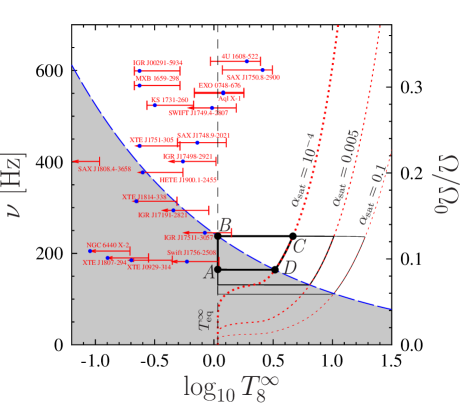
Figure 2: (color online) Spin frequency vs internal redshifted temperature for NSs in LMXBs. The frequencies and fiducial temperatures of 20 sources from Tab. 1 are shown by small filled circles. Error bars describe uncertainties in $T^{\infty}$ related to poorly constrained envelope composition (see Sec. III.1 and Table 1). Evolution tracks for a NS in LMXB are plotted by the solid lines (black online; thick, medium, and thin lines are for $\alpha_{\mathrm{sat}}=10^{-4}$, $0.005$, and $0.1$, respectively). Four points $A$, $B$, $C$, and $D$ separate different stages of NS evolution on the track, which corresponds to $\alpha_{\mathrm{sat}}=10^{-4}$. The stability region for $r^{o}$-mode with $m=2$ is filled with grey, its boundary is shown by thick dashed line (blue online). The vertical dashed line demonstrates the equilibrium stellar temperature $T_{\mathrm{eq}}^{\infty}$. The dotted lines (red online) are the Cooling=Heating curves for $\alpha_{\mathrm{sat}}=10^{-4}$, $0.005$, and $0.1$. See text for details.

The region of typical temperatures and spin frequencies for NSs in LMXBs is shown in Fig. 2. The small filled circles demonstrate the fiducial temperatures $T^{\infty}_{\rm fid}$ of the sources from Table 1, corresponding to the column depth of light elements $P/g=10^{9}$ g cm^-2. The error bars indicate uncertainties in the internal temperature, which can vary from $T_{\rm acc}^{\infty}$ (fully accreted envelope) to $T_{\rm Fe}^{\infty}$ (iron envelope), see Table 1. If only an upper limit for the effective temperature is known for a source, then the left error bar ends with arrow and the values of $T^{\infty}_{\rm fid}$, $T^{\infty}_{\rm acc}$, and $T^{\infty}_{\rm Fe}$ are calculated for that upper limit. Note that, because $\nu$ and $T^{\infty}_{\rm eff}$ for the sources EXO 0748-676 and Aql X-1 are very close to one another, the corresponding error bars almost merge in Fig. 2.

By dashes we plot the “instability curve” for the quadrupole $m=2$ $r^{o}$-mode, which is determined by the condition $1/\tau_{\rm GR}+1/\tau_{\rm Diss}=0$. Above this curve $1/\tau_{\rm GR}+1/\tau_{\rm Diss}<0$ and, as follows from Eq. (19), a star becomes unstable with respect to excitation of the $r^{o}$-mode ($d\alpha/dt>0$). This region is often referred to as the instability window for $r$-modes Andersson and Kokkotas (2001). The region filled with grey in the figure is the stability region for the $m=2$ $r^{o}$-mode. One can observe that a number of NSs appears well beyond the stability region.

As it was first shown by Levin Levin (1999) (see also Ref.  Heyl (2002)), NSs in LMXBs can undergo a cyclic evolution. This results in a closed track in the $\nu-T^{\infty}$ plane with a part of the track belonging to the instability region. For the NS model described in Sec. II and the $r^{0}$-mode saturation amplitude $\alpha_{\rm sat}=10^{-4}$ such a track $A$–$B$–$C$–$D$–$A$ is shown in Fig. 2 by the thick solid line (black online); medium and thin solid lines demonstrate similar tracks for $\alpha_{\rm sat}=5\times 10^{-3}$ and $\alpha_{\rm sat}=10^{-1}$, respectively. It is worth noting that, qualitatively, the shape of these tracks does not depend on the details of microphysics input adopted in Sec. II.

The evolution tracks in Fig. 2 consist of four main stages. Let us describe them briefly, taking the $A$–$B$–$C$–$D$–$A$ track as an example (a detailed discussion with a number of useful estimates can be found in Appendix B):

($i$) Spin-up of the star in the stability region at a temperature $T_{A}^{\infty}=T_{\rm eq}^{\infty}$ (stage $A$–$B$).

The star stays in the stability region and $r^{o}$-modes are not excited ($\alpha=0$). In accordance with Eq. (20), the spin frequency increases linearly with time due to accretion of matter onto the NS, while the stellar temperature $T^{\infty}$, governed by Eq. (16), stays constant. This stage lasts $\tau_{AB}\approx 4\times 10^{7}$ yr and ends by crossing the instability curve.

($ii$) Runaway heating of the star in the instability region (stage $B$–$C$).

This stage starts when the star leaves the $m=2$ $r^{o}$-mode stability region due to accretion-driven spin-up. The corresponding oscillation amplitude $\alpha$ begins to increase rapidly from the initial value determined by fluctuations (for example, the thermal fluctuations or those, related with accretion). Even at very low initial amplitude $\alpha=10^{-30}$ it takes $\Delta t_{\rm torq}\approx 4500$ yr for the torque associated with viscous damping of the $r^{o}$-mode to become equal to the accretion torque [$d\Omega/dt=0$, see Eq. (20)]. In the next $\approx 4$ yr, the $r^{o}$-mode reaches saturation ($\alpha=\alpha_{\rm sat}$). During these two periods of time, $T^{\infty}$ and $\Omega$ remain almost unchanged (the shift of the star in Fig. 2 is smaller than the width of the evolution track line).

Having reached saturation, the amplitude of $m=2$ $r^{o}$-mode stops growing and the star (within the time $\Delta t_{T}\approx 3000$ yr) warms up to the temperature, at which the neutrino emission exactly compensates the heating caused by the dissipation of the saturated oscillation mode [see Eq. (16)],

$$-\frac{\widetilde{J}MR^{2}\Omega^{2}\alpha_{\rm sat}^{2}}{\tau_{\rm GR}}-L_{\rm cool}+K_{\rm n}\dot{M}c^{2}=0.$$ (25)

The temperatures that satisfy this condition strongly depend on the stellar spin frequency and the saturation amplitude. We will refer to the corresponding curves in the $\nu-T^{\infty}$ plane as the Cooling=Heating curves; they are shown in Fig.  2 for $\alpha_{\rm sat}=10^{-4}$, $5\times 10^{-3}$, and $10^{-1}$ by the dotted lines (red online). These lines constrain the region of temperatures and frequencies accessible for NSs in LMXBs; the star cannot intersect the Cooling=Heating curve during its runaway, since this requires a more intensive heating than the dissipation of the saturated mode can provide. Note that the frequency remains almost unchanged during the $B$–$C$ stage.

($iii$) Spin-down of the star along the Cooling=Heating curve in the instability region (stage $C$–$D$).

Having reached point $C$, the star starts to move along the Cooling=Heating curve; that is, its temperature is determined by the balance of neutrino luminosity and heating due to dissipation of the saturated mode. As the rate of the angular momentum loss associated with the emission of gravitational waves is larger than the accretion torque in our NS model, the star starts to spin down. Eventually, the star returns into the stability region. This stage lasts $\Delta t_{CD}\approx 8\times 10^{6}$ yr.

($iv$) Cooling of the star in the stability region (stage $D$–$A$).

Having entered into the stability region, the $r^{o}$-mode amplitude vanishes rapidly (in $\sim 400$ yr), and after that a cooling of the star down to the temperature $T_{\rm eq}^{\infty}$ (point $A$) takes place. The cooling lasts $\sim 10^{5}$ yr, then the cycle repeats. The spin frequency does not change noticeably during the $D$–$A$ stage.

Summarizing, the star spends most of the time in stage ($i$) and only rarely gets into the instability region. Furthermore, in the instability region the star spends in stage ($ii$) a few orders of magnitude less time than in stage ($iii$).

Obviously, none of the observed NSs in LMXBs evolves along the tracks in Fig. 2. Various modifications of the standard scenario described above, for example, decreasing of $T_{\rm eq}^{\infty}$ (with the aim to increase $\Omega_{B}$) and increasing of the saturation amplitude $\alpha_{\rm sat}$, can allow one to interpret the observed sources as moving along the horizontal part of the evolution track that corresponds to stage ($ii$)—runaway heating of a star in the instability region. However, such modifications would make the detection of any source in this stage even more unlikely since they would further decrease the fraction of time spent there by the star Heyl (2002). In addition, this interpretation of observations would also suggest that a significant number of NSs in LMXBs should be located in stage ($iii$) (on the Cooling=Heating curve), since the duration of this stage is a few orders of magnitude larger than that of stage ($ii$) (see Appendix B). As follows from Fig. 2, the Cooling=Heating curves (the dotted lines; red online) correspond to very high temperatures ($T^{\infty}\sim 4\times 10^{8}$ K), so such stars should have been observed. Nevertheless, none of the NSs detected in LMXBs has a redshifted effective temperature larger than $T_{\mathrm{eff}}^{\infty}\gtrsim 2\times 10^{6}$ K (which corresponds to $T^{\infty}_{\rm fid}\gtrsim 4\times 10^{8}$ K for the canonical NS model).

In other words, the NS temperatures and frequencies inferred from the LMXB observations cannot be explained within the standard scenario. Therefore, to explain the sources from Fig. 2 one usually follows a different approach, trying to raise the instability curves so that all the sources would be contained inside the stability region. To this aim one needs to enhance dramatically the dissipation of the $m=2$ $r^{o}$-mode. Unfortunately, it is very difficult to justify such an enhancement from the microphysics point of view Ho et al. (2011); Haskell et al. (2012).

An alternative approach to the explanation of the sources with high temperatures and frequencies was suggested in Refs. Ho et al. (2011); Haskell et al. (2012); Mahmoodifar and Strohmayer (2013); Bondarescu and Wasserman (2013). It is based on the assumption that the NSs observed in the instability region are in the quasistationary state, in which the stellar temperature keeps constant ($dT^{\infty}/dt=0$) by balancing the neutrino cooling and heating associated with the dissipation of the saturated $r^{o}$-mode. However, to satisfy this condition the saturation amplitudes should differ substantially from source to source and, in addition, should have very low values of $\alpha_{\rm sat}\sim 10^{-9}$–$10^{-6}$, in disagreement with the recent calculations Bondarescu et al. (2007, 2009). According to the model of Refs. Bondarescu et al. (2007, 2009), the saturation amplitude is determined by the lowest parametric instability threshold among various triplets of the $r^{o}$-mode and two inertial daughter modes with which it is coupled nonlinearly. The threshold depends on the detuning of frequencies in the mode triplet and on the damping time scales of daughter modes. Since the mode frequencies are nonlinear functions of the spin frequency $\nu$, for some $\nu$ a very small detuning can occasionally occur for not very high daughter modes with relatively weak damping. It may thus lead to a very low saturation amplitude. However, such situation seems to be unstable, because the variation of the spin frequency increases detuning and the saturation amplitude and, as a result, additionally heats up the star.

Summarizing, to the best of our knowledge, all attempts to explain the significant number of rapidly rotating warm NSs have been made under rather artificial assumptions that either cannot be fully justified or even contradict the up-to-date calculations available in the literature.

IV Superfluid and normal modes

IV.1 Two main assumptions

In this section we formulate and discuss two main assumptions which are made in order to explain observations.

As it has been mentioned above, two types of inertial modes, superfluid and normal ones, exist in rotating NSs. Strictly speaking, these two types are clearly distinct only if one sets to zero the so-called coupling parameter $s$ Gusakov and Kantor (2011); Gusakov et al. (2013); Kantor and Gusakov (2013); Gualtieri et al. (2014). In the absence of other mechanisms of mode decoupling (see the end of this section), $s=s_{\rm EOS}$, where the parameter $s_{\rm EOS}$ depends only on an EOS of superdense matter and is given by Gusakov and Kantor (2011)

$$s_{\rm EOS}\equiv\frac{n_{e}}{n_{b}}\,\frac{\partial P(n_{b},\,n_{e})/\partial n_{e}}{\partial P(n_{b},\,n_{e})/\partial n_{b}}.$$ (26)

Here $n_{b}$ and $n_{e}$ are, respectively, the baryon and electron number densities. As it was shown in Refs. Gusakov and Kantor (2011); Kantor and Gusakov (2013), when $s$ vanishes, equations governing superfluid and normal modes decouple into two independent systems of equations. In this approximation, a system that describes the normal modes can be written in exactly the same form as for a nonsuperfluid star. Hence, the spectrum and eigenfunctions of normal modes coincide with the corresponding quantities of a normal star, and oscillation frequencies $\omega$ are independent of NS temperature $T^{\infty}$. Superfluid inertial modes, in turn, do not have a counterpart in normal stars; unlike the normal modes, $\omega$ for superfluid modes is a strong function of $T^{\infty}$.

In reality, the actual coupling parameter $s$ is small but finite (for example, for APR EOS $s_{\rm EOS}\sim 0.01$–$0.03$ Gusakov and Kantor (2011)). This leads to a strong interaction of normal and superfluid modes when their frequencies become close to one another. As a result, instead of crossings of these modes in the $\omega-T^{\infty}$ plane, one has avoided crossings: As $T^{\infty}$ varies, the superfluid mode turns into the normal mode and vice versa.

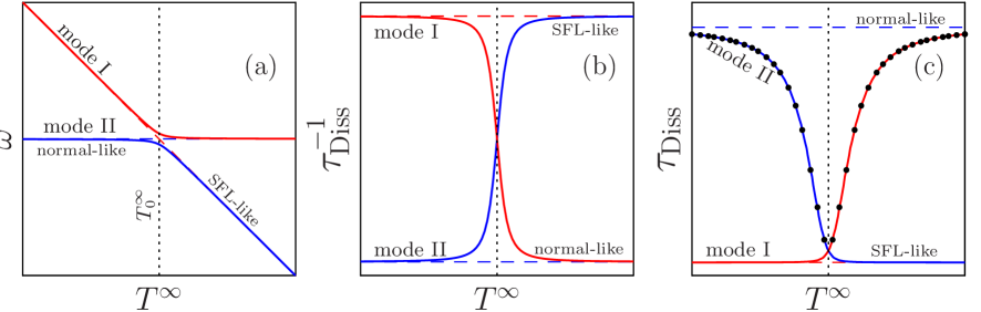
Figure 3: (color online) A schematic plot showing (a) oscillation frequencies, (b) inverse damping time scale $\tau^{-1}_{\rm Diss}$, and (c) $\tau_{\rm Diss}$ versus temperature $T^{\infty}$ for two oscillation modes (I and II) of a superfluid NS, which experience avoided crossing at $T^{\infty}=T_{0}^{\infty}$. Dashes correspond to an approximation of independent oscillation modes ($s=0$), solid lines are plotted for exact solution allowing for the interaction of modes I and II. The vertical dotted line indicates $T_{0}^{\infty}$. Filled circles in panel (c) illustrate the results shown in Fig. 12 of Ref. Lee and Yoshida (2003). See text for details.

These points are illustrated in Fig. 3(a) where we (schematically) present oscillation frequency $\omega$ as a function of $T^{\infty}$ for two neighboring modes of a superfluid NS (these modes are denoted as “I” and “II”, see the figure). At $T^{\infty}<T_{0}^{\infty}$, mode I behaves itself as a superfluid one (that is, its frequency depends on $T^{\infty}$), while mode II demonstrates the normallike behavior. At $T^{\infty}\approx T_{0}^{\infty}$, the frequencies of both modes come closer and equations describing superfluid and normal modes become strongly coupled. This results in an avoided crossing of modes: At $T^{\infty}>T_{0}^{\infty}$ mode II starts to behave as a superfluid mode while mode I becomes normallike. In contrast, assuming $s=0$, one would obtain crossing of modes instead of avoided crossing (see the dashed lines in the figure); in that case superfluid and normal modes would not “feel” each other.

The qualitative behavior of oscillation modes in superfluid NSs described above has been confirmed by direct calculation of radial Kantor and Gusakov (2011); Gusakov et al. (2013) and nonradial Gualtieri et al. (2014) oscillation modes. The concept of weakly interacting superfluid and normal modes has also been used in Refs. Chugunov and Gusakov (2011); Gusakov et al. (2013) for a detailed analysis of nonradial oscillation spectra of nonrotating NSs and damping of these oscillations.

Unfortunately, self-consistent calculations of oscillations of rotating superfluid NSs at finite temperatures are still unavailable in the literature. However, it seems natural that the behavior of inertial modes (in particular, $r$-modes) in superfluid NSs should be quite similar. The results of Refs. Lindblom and Mendell (2000); Yoshida and Lee (2003a, b); Lee and Yoshida (2003) provide indirect independent confirmation of this assumption (see below).

Thus, our first main assumption is

1. An oscillation mode of a superfluid rotating NS, which behaves, at some $T^{\infty}$, as a normal quadrupole $m=2$ $r$-mode ($r^{o}$-mode) can, as the temperature gradually changes, transform into a superfluidlike inertial mode ($i^{s}$-mode).

Our second main assumption is

2. Dissipative damping of a NS oscillation mode in the regime when it mimics the $m=2$ $r^{o}$-mode is much smaller than damping of this mode in the superfluid-like ($i^{s}$-mode) regime [see Figs. 3(b)–3(c), which show a qualitative dependence of the damping time scale $\tau_{\rm Diss}$ and its inverse $\tau_{\rm Diss}^{-1}$ on $T^{\infty}$ for the same two modes as in Fig. 3(a)].

What is the second assumption based on?

First, it is based on the analysis of $\tau_{\rm Diss}$ for nonradial oscillations of a nonrotating NS Gusakov et al. (2013); Gualtieri et al. (2014). As it was demonstrated in Ref. Gusakov et al. (2013), damping of oscillation modes due to the shear viscosity in the superfluidlike regime occurs approximately ten times faster than their damping in the normallike regime. The reasons for that are discussed in detail in Sec. 7.4 of Ref. Gusakov et al. (2013) and should be applicable to $r$-modes. This is also in line with the results of Refs. Lee and Yoshida (2003); Yoshida and Lee (2003a), where it was found that $\tau_{\rm S}$ for the zero-temperature $i^{s}$-modes is generally more than 1 order of magnitude smaller than for normal $r^{o}$-modes (compare Table 1 of Ref. Lee and Yoshida (2003) and Table 2 of Ref. Yoshida and Lee (2003a)).

But the main dissipation mechanism, which leads to a drastic difference (by orders of magnitude) of $\tau_{\rm Diss}$ in superfluid- and normallike regimes, is the mutual friction between the superfluid and normal matter components Alpar et al. (1984); Mendell (1991); Andersson et al. (2006). The friction occurs because of electron scattering off the magnetic field of Feynman-Onsager vortices. The corresponding magnetic field is generated because of entrainment Andreev and Bashkin (1975) of superconducting protons by the motion of superfluid neutrons.

This mechanism tends to equalize the velocities of normal and superfluid components; it does not noticeably affect dissipation of the normal modes, since for normal modes these velocities approximately coincide (comoving motion). On the opposite, mutual friction is extremely effective for superfluid modes, because in that case the difference between the normal and superfluid velocities is large (countermoving motion). In application to $r$-modes the effects of mutual friction were studied in detail in Refs. Lindblom and Mendell (2000); Lee and Yoshida (2003); Andersson et al. (2009); Haskell et al. (2009). In particular, the damping time scale for normal $r$-modes ($r^{o}$-modes) due to mutual friction was shown to be

$$\frac{1}{\tau^{\rm norm}_{\rm MF}}=\frac{1}{\tau^{\rm norm}_{{\rm MF}\,0}}\,\left(\frac{\Omega}{\Omega_{0}}\right)^{5},$$ (27)

where $\tau_{{\rm MF}\,0}^{\rm norm}\sim 10^{3}$–$10^{4}$ s Lindblom and Mendell (2000); Lee and Yoshida (2003). Superfluid $r$-modes ($r^{s}$-modes) and superfluid inertial modes ($i^{s}$-modes) were studied, for the first time, in Refs. Lee and Yoshida (2003) and Yoshida and Lee (2003a), respectively; for the damping time scale of these modes due to mutual friction they obtain

$$\frac{1}{\tau^{\rm sfl}_{\rm MF}}=\frac{1}{\tau^{\rm sfl}_{{\rm MF}\,0}}\,\frac{\Omega}{\Omega_{0}},$$ (28)

where $\tau^{\rm sfl}_{{\rm MF}\,0}\sim 0.1$ s (see Table 1 in Ref. Lee and Yoshida (2003) and Table 2 in Ref. Yoshida and Lee (2003a)). It is interesting that $i^{s}$-modes were also presumably found in Ref. Lindblom and Mendell (2000) (see the resonances in their Fig. 6 and the corresponding discussion in that reference).

The results obtained by Lee and Yoshida Lee and Yoshida (2003); Yoshida and Lee (2003a) indirectly confirm our main assumptions 1 and 2. These authors employed the zero temperature approximation ($T^{\infty}=0$) and varied the so-called “entrainment” parameter $\widetilde{\eta}$ ($\eta$ in their paper), that parametrizes interaction between the superfluid neutrons and superconducting protons. It follows from the microphysics calculations Gusakov and Haensel (2005); Gusakov et al. (2009); Gusakov (2010) that $\widetilde{\eta}$ is a function of $T^{\infty}$. Hence, its variation is analogous to a variation of stellar temperature. In other words, the eigenfrequencies and eigenfunctions for the superfluid oscillation modes should depend on $\widetilde{\eta}$, while these for the normal modes should be almost insensitive to this parameter. Thus, all the peculiarities in the behavior of oscillation modes with changing $T^{\infty}$ discussed above should also be observed in calculations of Refs. Lee and Yoshida (2003); Yoshida and Lee (2003a), where $\widetilde{\eta}$ is varied. (In particular, Fig. 3 should still be applicable, provided that one replaces $T^{\infty}$ with $\widetilde{\eta}$ there.)

And indeed, Lee and Yoshida Lee and Yoshida (2003); Yoshida and Lee (2003a) found numerous avoided crossings of superfluid and normal inertial modes (see their Figs. 5–8 in Ref. Yoshida and Lee (2003a)). Concerning $r$-modes, in Ref. Lee and Yoshida (2003) they found avoided crossing between the $m=2$ $r^{s}$-mode and one of the normal inertial $i^{o}$-modes (see their Fig. 7) and crossings of the $m=2$ $r^{o}$-mode with two superfluid inertial modes (see their Fig. 8). In the latter case, Lee and Yoshida emphasized on p. 409 that “it is quite difficult to numerically discern whether the mode crossings result in avoided crossings or degeneracy of the mode frequencies at the crossing point.” If our interpretation is correct, there should be avoided crossings.

This point of view is supported by Fig. 12 of the same Ref. Lee and Yoshida (2003). The figure shows the time scale $\tau_{{\rm MF}\,0}$ [corresponding to our time $\tau_{\rm MF\,0}^{\rm norm}$, introduced in Eq. (27)] for the $m=2$ $r^{o}$-mode as a function of $\widetilde{\eta}$ for the same stellar parameters as in Fig. 8 of that reference. One can see that $\tau_{{\rm MF}\,0}$ in Fig. 12 sharply decreases (by a few orders of magnitude) at the values of $\widetilde{\eta}$ at which one observes crossing of the $r^{o}$- and $i^{s}$-modes in Fig. 8. This is exactly what one would expect if our assumptions 1 and 2 are correct. Near the crossing of modes (which is avoided crossing in reality) the $m=2$ $r^{o}$-mode starts to transform into the $i^{s}$-mode, and hence $\tau_{{\rm MF}\,0}$ drops down rapidly. Moving away from the avoided crossing (by decreasing or increasing $\widetilde{\eta}$) the solution found by Lee and Yoshida resembles more and more the $m=2$ $r^{o}$-mode. Consequently, $\tau_{{\rm MF}\,0}$ grows on both sides of the resonance, approaching the asymptote value corresponding to the pure (with no admixture) $m=2$ $r^{o}$-mode. The results obtained in Fig. 12 of Ref. Lee and Yoshida (2003) are shown qualitatively by filled circles in our Fig. 3(c).

The fact that Lee and Yoshida Lee and Yoshida (2003) fail to discriminate between crossing and avoided crossing of modes in their Fig. 8 indicates that the real coupling parameter $s$ responsible for the interaction of $m=2$ $r^{o}$- and $i^{s}$-modes is actually much smaller than the parameter $s_{\rm EOS}$ given by Eq. (26). The reason is the stellar matter only weakly deviates from the beta-equilibrium state in the course of the $m=2$ $r^{o}$-mode oscillations [the deviation $\delta\mu\sim(\Omega/\Omega_{0})^{4}$ Lindblom and Mendell (2000) is small since $\Omega\ll\Omega_{0}$]. It can be shown Gusakov and Kantor (2011); Gusakov et al. (2013); Kantor and Gusakov (2013); Gualtieri et al. (2014) that in that case the superfluid degrees of freedom decouple from the normal ones especially well. According to our preliminary estimates, the real coupling parameter can be of the order of $s\sim s_{\rm EOS}\,(\Omega/\Omega_{0})^{2}$. If this estimate is correct then for $s_{\rm EOS}=0.01$ and $\Omega/\Omega_{0}=0.1$ one has $s\sim 10^{-4}$. However, in view of the existing uncertainties, in this paper we adopt the larger value, $s=0.001$. We checked that the variation of $s$ within the very wide range (by orders of magnitude) does not affect our principal results.

IV.2 Mixing the modes

Obviously the fact that the real oscillation modes of superfluid NSs demonstrate, depending on $T^{\infty}$, either normal- or superfluidlike behavior should have a major effect on the stability region discussed in Sec. III.2. To describe this effect it is necessary to understand how the time scales $\tau_{\rm S}$, $\tau_{\rm MF}$, and $\tau_{\rm GR}$ are modified during the transformation of the mode from the normallike to superfluidlike regime (see Fig. 3). Since there are no accurate calculations of these time scales in the literature, below we develop a simple phenomenological model evoked by the perturbation theory of quantum mechanics.

Assume for a moment that the coupling parameter $s=0$, so that the systems of equations describing the superfluid and normal oscillation modes are completely decoupled. The solution to these systems of equations describes two types of independent modes, the superfluid and normal ones. Let us present the eigenfunctions of normal modes in the form of a column vector $\Psi_{\rm norm}$ and those of superfluid modes in the form of a column vector $\Psi_{\rm sfl}$. Assume further that $\Psi_{\rm norm}$ and $\Psi_{\rm sfl}$ are normalized by the one and the same oscillation energy $E_{\rm c}$ and that the time scale $\tau_{X}$ of damping/excitation of oscillations due to some dissipation mechanism [e.g., shear viscosity ($X={\rm S}$), mutual friction ($X={\rm MF}$), or gravitational radiation ($X={\rm GR}$)] is given by the general formula of the form

$$\frac{1}{\tau_{X}}=-\frac{1}{2E_{\rm c}}\,\frac{dE_{\rm c}}{dt}=-\frac{1}{2E_{\rm c}}\,(\Psi,\,\hat{A}\,\Psi),$$ (29)

where $\hat{A}$ is a matrix differential operator and $(\Psi_{1},\,\Psi_{2})$ is a scalar product, both specified by the actual mechanism of dissipation. For example, for $X={\rm S}$ or MF the scalar product is defined as (e.g., Ref. Yoshida and Lee (2003a))

$$(\Psi_{1},\Psi_{2})\equiv\int_{\rm star}\Psi_{1}^{\dagger}\,\Psi_{2}\,dV,$$ (30)

where the integration is performed over the NS volume $V$. To determine the time scale $\tau_{X}^{\rm norm}$ for normal modes one should set $\Psi\equiv\Psi_{\rm norm}$ in Eq. (29); similarly, to determine the time scale $\tau_{X}^{\rm sfl}$ for superfluid modes one should assume $\Psi\equiv\Psi_{\rm sfl}$. Note that for normal $r$-modes the time scales $\tau_{\rm GR}^{\rm norm}$ and $\tau_{\rm S}^{\rm norm}$ have been already calculated in Sec. II and are given by, respectively, Eqs. (9) and (13).

As has been mentioned above, in reality the parameter $s$ is small but finite. This means that the eigenfunctions $\Psi_{\rm norm}$ and $\Psi_{\rm sfl}$ approximate well the exact solution far from the avoided crossings of neighboring modes ($\Psi_{\rm norm}$ describes well the exact solution in the normallike regime, while $\Psi_{\rm sfl}$ does so in the superfluidlike regime). However, in the vicinity of an avoided crossing the eigenfunctions of the exact solution should be presented as a linear superposition of $\Psi_{\rm norm}$ and $\Psi_{\rm sfl}$. In particular, in Fig. 3 avoided crossing occurs between modes I and II. Denoting the corresponding eigenfunctions as $\Psi_{\rm I}$ and $\Psi_{\rm II}$, one can write

$$\Psi_{\rm I} = -{\rm sin}\theta(x)\,\Psi_{\rm norm}+{\cos}\theta(x)\,\Psi_{\rm sfl},$$ (31)

$$\Psi_{\rm II} = ~{}~{}\,{\rm cos}\theta(x)\,\Psi_{\rm norm}+{\sin}\theta(x)\,\Psi_{\rm sfl},$$ (32)

where ${\cos}\theta(x)$ and ${\sin}\theta(x)$ guarantee the correct normalization of the eigenfunctions $\Psi_{\rm I}$ and $\Psi_{\rm II}$ by the oscillation energy $E_{\rm c}$, while the function $\theta(x)$ determines how the normal mode transforms into the superfluid one (and vice versa). This function depends on the parameter $x\equiv(T^{\infty}-T_{0}^{\infty})/\Delta T^{\infty}$ [see Fig. 3(a)] and ranges from $0$ to $1$ on a temperature scale specified by the characteristic width $\Delta T^{\infty}$ of the avoided crossing, $\Delta T^{\infty}\sim s\,T^{\infty}_{0}$. The exact form of the function $\theta(x)$ can be found only by direct solution to the coupled oscillation equations. However, using as the analogy the problem of intersection of electron terms in molecules (see, e.g., Ref. Landau and Lifshits (1977), Sec. 79), one can immediately write down an approximate expression for $\theta(x)$ that correctly reproduces its main properties,

$$\theta(x)=\frac{1}{2}\left[\frac{\pi}{2}+\arctan(x)\right].$$ (33)

Consider, for example, mode II. At $x\rightarrow-\infty$ one has $\theta(x)\rightarrow 0$, and it follows from Eq. (32) that mode II is in the normallike regime ($\Psi_{\rm II}=\Psi_{\rm norm}$); at $x\rightarrow+\infty$ one obtains $\theta(x)\rightarrow\pi/2$, which corresponds to superfluidlike behavior of mode II ($\Psi_{\rm II}=\Psi_{\rm sfl}$).

Now, substituting Eqs. (31) and (32) into (29) and neglecting the interferential terms of the form

$$-\frac{1}{2E_{\rm c}}\,\,\,{\cos}\theta(x)\,{\sin}\theta(x)\,(\Psi_{\rm norm},\,\hat{A}\,\Psi_{\rm sfl}),$$ (34)

one gets

$$\frac{1}{\tau_{X}}\approx\frac{1}{\tau_{X}^{\rm norm}}\,{\sin}^{2}\theta(x)+\frac{1}{\tau_{X}^{\rm sfl}}\,{\cos}^{2}\theta(x)$$ (35)

for mode I and

$$\frac{1}{\tau_{X}}\approx\frac{1}{\tau_{X}^{\rm norm}}\,{\cos}^{2}\theta(x)+\frac{1}{\tau_{X}^{\rm sfl}}\,{\sin}^{2}\theta(x)$$ (36)

for mode II. These are the main formulas of our approximate model. Their use for $X={\rm S,\,MF,\,GR}$ enables us to plot the instability windows for the real oscillation modes (similar to modes I and II shown in Fig. 3).

V Realistic instability windows and three-mode regime

V.1 Realistic instability windows

Let us assume that a certain oscillation mode of a rotating superfluid NS (by analogy with the previous section we will refer to it as mode II) behaves like the $m=2$ $r^{o}$-mode at low temperatures, and that at $T^{\infty}=T^{\infty}_{0}$ it experiences an avoided crossing with another mode (with the same $m=2$, let us call it mode I), which behaves like a superfluid inertial mode ($i^{s}$-mode) at low $T^{\infty}$ (exactly as in the scheme in Fig. 3). After avoided crossing, mode I starts to behave as an $m=2$ $r^{o}$-mode, and mode II as an $i^{s}$-mode. Let us determine the instability windows for these modes.

The instability windows are defined by the following inequality (see also Sec. III.2 above):

$$\frac{1}{\tau_{\rm GR}}+\frac{1}{\tau_{\rm S}}+\frac{1}{\tau_{\rm MF}}<0.$$ (37)

Each of these times cales can be calculated using Eq. (36) for mode II and Eq. (35) for mode I. One only needs to specify the values for $\tau_{X}^{\rm norm}$ and $\tau_{X}^{\rm sfl}$, which will be employed in each case.

($i$) Shear viscosity ($X={\rm S}$). The damping time scale $\tau_{\rm S}^{\rm norm}$ for the $m=2$ $r^{o}$-mode is determined by Eq. (13). According to the discussion in Sec. IV.1, $\tau_{\rm S}^{\rm sfl}$ for the $i^{s}$-mode is taken to be

$$\tau_{\rm S}^{\rm sfl}=c_{\rm S}\,\tau_{\rm S}^{\rm norm},$$ (38)

where $c_{\rm S}=0.1$. Since the mutual friction dissipation dominates for the superfluid $i^{s}$-mode [see item ($ii$) below and compare Eqs. (28) and (38)], the specific value of the coefficient $c_{\rm S}$ is not important for our scenario; one can take $1$ or $0.01$ instead of $0.1$, and the main results will not change.

($ii$) Mutual friction ($X={\rm MF}$). The damping time scale $\tau_{\rm MF}^{\rm norm}$ is given by Eq. (27) with $\tau_{\rm MF\,0}^{\rm norm}=10^{4}$ s; the time $\tau_{\rm MF}^{\rm sfl}$ is determined from Eq. (28) with $\tau_{\rm MF\,0}^{\rm sfl}=2.5$ s. Our scenario is insensitive to the actual choice of $\tau_{\rm MF\,0}^{\rm norm}$ because the mutual friction is not a dominating dissipative process for normal modes. However, it is crucial that $\tau_{\rm MF\,0}^{\rm sfl}$ be sufficiently small, $\tau_{\rm MF\,0}^{\rm sfl}\lesssim 100$ s.

($iii$) Gravitational radiation ($X={\rm GR}$). The time scale $\tau_{\rm GR}^{\rm norm}$ is given by Eq. (9); $\tau_{\rm GR}^{\rm sfl}$ is taken to be

$$\tau_{\rm GR}^{\rm sfl}=c_{\rm GR}\,\tau_{\rm GR}^{\rm norm},$$ (39)

where $c_{\rm GR}=100$. Such an expression for the gravitational radiation time scale for the $i^{s}$-mode agrees qualitatively with the results of Refs. Lee and Yoshida (2003); Yoshida and Lee (2003a) [see Eq. (44) and Table 2 of Ref. Yoshida and Lee (2003a)], where even longer time scales were obtained, corresponding to $c_{\rm GR}>10^{4}$(see also Gualtieri et al. (2014)). For readability of Fig. 4(a) we take $c_{\rm GR}=100$, thus underestimating $\tau_{\rm GR}^{\rm sfl}$ for the $m=2$ $i^{s}$-mode significantly. Increasing of $c_{\rm GR}$ (and even further decreasing of $c_{\rm GR}$ down to $\sim 1$) does not affect the scenario suggested in this paper.

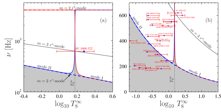
Figure 4: (color online) Instability curves for superfluid NS oscillations. The solid curves correspond to $m=2$ modes I and II (red and blue online, respectively), which experience avoided crossing at $T_{0}^{\infty}=1.5\times 10^{8}$ K. The coupling parameter was chosen to be $s=0.001$. The dashed curves correspond to the $m=2$ $r^{o}$- and $i^{s}$-modes (blue and red online, respectively) plotted under the assumption that they are completely decoupled ($s=0$). The grey line is the instability curve for the $m=3$ $r^{o}$-mode, plotted ignoring the resonance coupling with the superfluid modes. The temperature $T_{0}^{\infty}$ is shown by the vertical dotted line. Similar to Fig. 2, the panel (b) shows temperatures and frequencies of the sources from Table 1. Only the fastest source 4U 1608-522 is shown in the panel (a). See text for details.

Instability curves for modes I (solid line; red online) and II (solid line; blue online) are shown in Figs. 4(a)–4(b). The curves are obtained by making use of Eqs. (35)–(39) with the coupling parameter $s=0.001$. Panel (b) is a version of panel (a), but plotted in a different scale. The dotted line in Figs. 4(a)–4(b) corresponds to the temperature $T^{\infty}_{0}=1.5\times 10^{8}$ K, at which the modes I and II experience avoided crossing. In addition, Figs. 4(a)–4(b) show the instability curves for ($i$) octupole $m=3$ $r^{o}$-mode (grey solid line; to plot it, we take the characteristic time scales $\tau_{\rm S}$ and $\tau_{\rm GR}$ from Sec. II and ignore the mutual friction, $\tau_{\rm MF}\equiv\infty$); ($ii$) $m=2$ $r^{o}$-mode (dashed line; blue online); ($iii$) superfluid $i^{s}$-mode with $m=2$ (dashed line; red online). The latter curves ($i$)–($iii$) are obtained using the approximation $s=0$ (neglecting the interaction between the superfluid and normal modes).

As one would expect, far from the avoided crossing point the solid (modes I and II) and dashed ($r^{o}$ and $i^{s}$-modes) lines almost coincide. The region where $m=2$ modes I, II, and the octupole $m=3$ $r^{o}$-mode are simultaneously stable is filled with grey in Figs. 4(a)–4(b). The presence of the “stability peak” at $T^{\infty}\approx T_{0}^{\infty}$ is an important characteristic feature of this region. The height of the peak is determined by the lowest-frequency intersection of the mode II instability curve with the other instability curves. The instability curves for modes I and II intersect at a very high frequency $\nu\approx 1580$ Hz; hence, the lowest-frequency intersection corresponds to that with the octupole $m=3$ $r^{o}$-mode and occurs at $\nu\approx 625$ Hz. As a result, at $T^{\infty}=T_{0}^{\infty}$ the most unstable mode is the $m=3$ $r^{o}$-mode, and the height of the stability peak is $\nu\approx 625$ Hz.

As follows from Fig. 4, the evolution of a NS with such a complicated structure of instability windows can be accompanied by excitation of each of the three oscillation modes. Therefore, prior to discussing the evolution tracks one should formulate the equations describing an oscillating star in a three-mode regime.

V.2 Three-mode regime

The equations governing the evolution of a NS and allowing for possible excitation of the three modes (I, II, and $m=3$ $r^{o}$-mode) can be derived in much the same fashion as it was done in Sec. II [see the one-mode equations (16), (19), and (20) in that section]. If all the modes are nonsaturated, they can be written as

$$\frac{d\alpha_{i}}{dt} = -\alpha_{i}\left(\frac{1}{\tau_{{\rm GR}\,i}}+\frac{1}{\tau_{{\rm Diss}\,i}}\right),$$ (40)

$$\frac{d\Omega}{dt} = -\sum_{i}\frac{2\,Q_{i}\,\alpha_{i}^{2}\,\Omega}{\tau_{{\rm Diss}\,i}}+\dot{\Omega}_{\rm acc},$$ (41)

$$C_{\rm tot}\frac{dT^{\infty}}{dt} = \sum_{i}W_{{\rm Diss}\,i}-L_{\rm cool}+K_{\rm n}\dot{M}c^{2},$$ (42)

where we neglect the terms $\propto\alpha_{i}^{3}$. The index $i$ in Eqs. (40)–(42) runs over the mode types, and

$$W_{{\rm Diss}\,i} = \frac{2E_{{\rm c}\,i}}{\tau_{{\rm Diss}\,i}},$$ (43)

$$\frac{1}{\tau_{{\rm Diss}\,i}} = \frac{1}{\tau_{{\rm S}\,i}}+\frac{1}{\tau_{{\rm MF}\,i}},$$ (44)

where $\tau_{{\rm S}\,i}$ and $\tau_{{\rm MF}\,i}$ for modes I and II are calculated as it is described in Sec. V.1, while for the octupole $m=3$ $r^{o}$-mode they are calculated as described in Sec. II (we neglect the effects of mutual friction on damping of the octupole $r^{o}$-mode).

Thus, only the quantities $E_{{\rm c}\,i}$ and $Q_{i}$ in Eqs. (41) and (43) are left to be determined. The corresponding Eqs. (18) and (22) for the octupole $r^{o}$-mode are presented in Sec. II. In the case of modes I and II one can argue as follows. First, let us discuss mode II. At low $T^{\infty}$ (before the avoided crossing), it behaves like the $m=2$ $r^{o}$-mode. Accordingly, its canonical angular momentum $J_{{\rm c}\,{\rm II}}$ is given by Eq. (6), where the coefficient $\widetilde{J}\approx 1.6353\times 10^{-2}$. At the avoided crossing point the behavior of the mode changes and it turns into the $i^{s}$-mode. However, since the canonical angular momentum is an adiabatic invariant Friedman and Schutz (1978b); Ho and Lai (2000); Wagoner (2002), $J_{{\rm c}\,{\rm II}}$ is conserved (neglecting dissipative processes) and stays the same even after passing the avoided crossing. Without any loss of generality, one can assume it to be still related to the oscillation amplitude $\alpha_{\rm II}$ by exactly the same Eq. (6) (with the same $\widetilde{J}=1.6353\times 10^{-2}$), as before the avoided crossing. This assumption, which should be treated as the definition of the amplitude $\alpha_{\rm II}$ in the superfluidlike regime, has already been implicitly employed when deriving the system of Eqs. (40)–(42). It ensures that $\alpha_{\rm II}$ is continuous throughout the avoided crossing region.

The same reasoning also holds true for mode I. For a given $J_{{\rm c}\,i}$ the quantities $Q_{i}$ and $E_{{\rm c}\,i}$ can be found from Eqs. (18) and (22). The problem, however, consists in that the mode energy $E_{{\rm c}\,i}$ depends on the oscillation frequency $\omega$, which is only known for modes I and II in the normallike regime [in that case, it is given by Eq. (2)]. In the superfluidlike regime, $\omega$ depends not only on $\Omega$, but also on $T^{\infty}$; unfortunately, the function $\omega(\Omega,\,T^{\infty})$ has not yet been calculated. Below, for simplicity, we assume that the frequency $\omega$ is determined by the same Eq. (2) even in the superfluidlike regime. This assumption does not influence our main conclusions and is well justified because the range of $T^{\infty}$, which is of interest in our scenario (see Sec. VI), is located near avoided crossings of modes. In that region $\omega$ for both modes can indeed be estimated from Eq. (2). Beyond this region any mode in the superfluidlike regime is stable, unexcited, and, correspondingly, not important for NS evolution.

Equations (40)–(42) are satisfied if the oscillation amplitudes $\alpha_{i}$ are less than the correspondent saturation amplitudes $\alpha_{{\rm sat}\,i}$. In the following, the saturation amplitudes for all the modes are taken to be $\alpha_{{\rm sat}\,i}=10^{-4}$ . Note that our main results are insensitive to the actual value of $\alpha_{{\rm sat}\,i}$. If one or more modes are saturated, the evolution equations can be derived in a similar way as it was done in Sec. II.

VI Our resonance uplift scenario

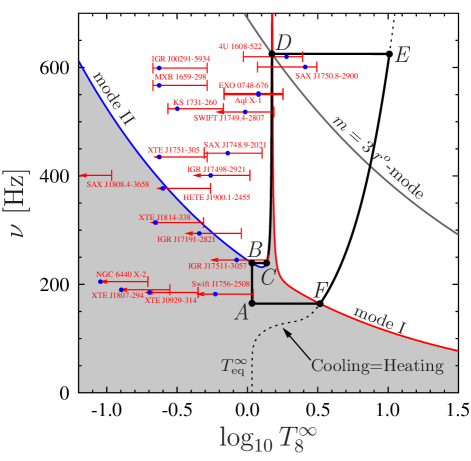
Figure 5: (color online) Evolution of the spin frequency $\nu$ and temperature $T^{\infty}_{8}$ for a superfluid NS in LMXB allowing for the avoided crossing of $m=2$ modes I and II. The corresponding track $A$–$B$–$C$–$D$–$E$–$F$–$A$ is shown by the thick solid line. The dotted line shows the Cooling=Heating curve (see text for details). Other notations are the same as in Fig. 4.

Using the results of the preceding sections, we can examine quantitatively how the resonance coupling of superfluid and normal modes modifies the standard scenario discussed in Sec. III.2 (see also Fig. 2).

A typical NS evolution track $A$–$B$–$C$–$D$–$E$–$F$–$A$ is shown in Fig. 5 by the thick solid line, calculated for exactly the same model as the instability curves in Sec. V.1 (see Fig. 4). Other notations coincide with those in Fig. 4. As in Sec. V.1, we suppose that mode I experiences an avoided crossing with mode II at $T^{\infty}=T_{0}^{\infty}=1.5\times 10^{8}$ K.

To plot the Cooling=Heating curve (shown by the dotted line in Fig. 5), we use Eq. (42) with $dT^{\infty}/dt=0$. When doing this we assume that all the modes, which are unstable at a given temperature and frequency, are saturated, while the stable modes have vanishing oscillation amplitudes. This means that in each point of the Cooling=Heating curve the neutrino luminosity is exactly compensated by the stellar heating due to nonlinear damping of saturated modes. Let us note that in the stability region (the grey-filled area in the figure) we do not use this definition, but instead, by analogy with Fig. 2, continue the Cooling=Heating curve according to Eq. (25). A break of the Cooling=Heating curve at the intersection point with the instability curve for the $m=3$ $r^{o}$-mode is imperceptible, because the contribution of the octupole mode to stellar heating can be neglected owing to a longer gravitational radiation time scale for this mode [see Eq. (9)]. Therefore, along the whole Cooling=Heating curve, the nonlinear damping of mode I, behaving as the saturated $m=2$ $r^{o}$-mode, is the dominating heating mechanism. This means that the Cooling=Heating curve, obtained while allowing for the resonance coupling of modes, is practically indistinguishable from that given by Eq. (25) (see Sec. III.2 and Fig. 2).

During the $A$–$B$ stage, a NS stays inside the stability region and gradually spins up by accretion. This stage is completely analogous to the $A$–$B$ stage of the standard scenario shown in Fig. 2. At point $B$, the star becomes unstable with respect to excitation of mode II, which behaves there as the $m=2$ $r^{o}$-mode. In the next stage $B$–$C$ the amplitude of mode II increases and rapidly reaches saturation ($\alpha_{\rm sat}=10^{-4}$). After that, the star heats up without any significant variation of the spin frequency $\nu$. This stage ends by reaching the stability peak at point $C$.

The next stage $C$–$D$ is the most interesting and is absent in the standard scenario described in Sec. III.2. Owing to accretion, the star is spinning up along the boundary of the stability peak produced by the avoided crossing of modes I and II. This stage is discussed in detail below. At point $D$ the star, for the first time, becomes unstable with respect to excitation of the octupole $m=3$ $r^{o}$-mode. The amplitude of this mode increases rapidly and hits saturation, which leads to heating up of the star. As a result, it leaves the stability peak, becomes unstable also with respect to excitation of mode I, and quickly moves to point $E$. Thus, the $D$–$E$ stage is quite similar to the $B$–$C$ stage of the standard scenario with the only difference that the two modes ($m=3$ $r^{o}$-mode and the mode I) are excited (and saturated) in this stage instead of one. The spin frequency is almost constant during this stage. At point $E$, the star approaches the Cooling=Heating curve and then spins down along this curve until it enters the stability region at point $F$ (stage $E$–$F$). All the oscillation modes vanish in the very beginning of the subsequent stage $F$–$A$ and the star cools down to the equilibrium temperature $T_{\rm eq}^{\infty}$ without noticeable variation of the spin frequency. Stages $E$–$F$ and $F$–$A$ are close analogues of, respectively, stages $C$–$D$ and $D$–$A$ of the standard evolution scenario (see Fig. 2).

Let us return to the almost vertical stage $C$–$D$ in Fig. 5 and discuss it in more detail. During this stage, the NS moves along the instability curve for mode II. Only mode II is excited; the amplitudes of other modes are all equal to zero. Since in stage $C$–$D$ the stellar temperature $T^{\infty}>T^{\infty}_{\mathrm{eq}}$, the star requires an additional heating to maintain its thermal balance. This heating is provided by the damping of mode II. A required power is determined from Eq. (42) by setting $dT^{\infty}/dt\approx 0$,

$$W_{{\rm Diss}\,\mathrm{II}}\approx L_{\rm cool}-K_{\rm n}\,\dot{M}\,c^{2}.$$ (45)

Using Eqs. (43) and (45), together with Eqs. (6) and (18), one can determine the corresponding equilibrium oscillation amplitude

$$\alpha^{\rm(eq)}_{\mathrm{II}}\approx\sqrt{\frac{(L_{\rm cool}-K_{\rm n}\,\dot{M}\,c^{2})\,\tau_{{\rm Diss\,II}}}{\widetilde{J}\,M\,R^{2}\,\Omega^{2}}},$$ (46)

where $\widetilde{J}\approx 1.6353\times 10^{-2}$ for mode II. Since $\tau_{{\rm Diss}\,{\rm II}}=-\tau_{{\rm GR}\,{\rm II}}$ on the instability curve, one can use $-\tau_{{\rm GR}\,{\rm II}}$ instead of $\tau_{{\rm Diss}\,{\rm II}}$ in this equation. For example, taking the point on the instability curve with coordinates $\nu=400$ Hz and $T^{\infty}\approx 1.48\times 10^{8}$ K, we obtain $L_{\rm cool}\approx 3.3\times 10^{34}$ erg s^-1; $\tau_{{\rm Diss}\,{\rm II}}=-\tau_{{\rm GR}\,{\rm II}}\approx 1.13\times 10^{4}$ s; and, as follows from Eq. (46), $\alpha^{\rm(eq)}_{\mathrm{II}}\approx 8\times 10^{-7}\ll\alpha_{\rm sat\,II}=10^{-4}$(note that, when climbing the peak $L_{\mathrm{cool}}$ stays almost constant; hence, the equilibrium amplitude scales as $\alpha^{\rm(eq)}_{\mathrm{II}}\propto\nu^{-4}$, because $\tau_{\rm GR\,II}\propto\nu^{-6}$).

It is possible for a star to maintain a finite, but not saturated oscillation amplitude for a long time, because it penetrates into the instability region with decreasing $T^{\infty}$. Indeed, if, for some reason, mode II has a lower amplitude than that required by Eq. (46), then the star starts to cool down and becomes unstable with respect to excitation of mode II. This immediately leads to increasing of the amplitude $\alpha_{\rm II}$ and to accelerated heating of the star. As a result, the star moves toward the stability region, where $\alpha_{\rm II}$ decreases rapidly, the heating becomes less and less efficient and, eventually, heating is replaced by cooling. The process of modulation of $\alpha_{\rm II}$ may occur repeatedly, but the correspondent variation of $T^{\infty}$ is very small. The characteristic modulation period varies from a few months to years.

It can be shown that the modulation magnitude may decrease or increase in time depending on the parameters of the model. In the first case, during the NS motion along the peak, the amplitude of mode II adjusts itself to the equilibrium value $\alpha_{\rm II}\approx\alpha^{\rm(eq)}_{\mathrm{II}}$ and does not experience modulation. In the second case, the maximum value of $\alpha_{\rm II}$ is typically limited by the saturation amplitude ($\alpha_{\rm II}=\alpha_{\rm sat\,II}$), thus limiting the modulation magnitude. However, even in this case the temperature oscillations accompanying the modulation are very small, less than the thickness of the line in Fig. 5, and can hardly be observed. At the same time, strong modulation of the oscillation amplitude $\alpha_{\rm II}$ is also accompanied by the modulation of $d\Omega/dt$, which is, in principle, observable. The effects of $\alpha_{\rm II}$ modulation described above will be discussed in detail in our subsequent publication.

Let us estimate the duration of the spin-up stage $C$–$D$. Using Eqs. (41) and (46), we get

$$\frac{d\Omega}{dt}=-\frac{2\,Q_{\rm II}\,(L_{\rm cool}-K_{\rm n}\,\dot{M}\,c^{2})}{\widetilde{J}\,M\,R^{2}\,\Omega}+\dot{\Omega}_{\rm acc},$$ (47)

where $Q_{\rm II}\approx 0.094$ [see Eq. (22)]. First of all, taking into account Eq. (21) one can determine from this formula the minimal NS accretion rate $\dot{M}_{\rm min}$ required to spin up the star,

$$\dot{M}_{\rm min} = \frac{3L_{\rm cool}}{3\,K_{\rm n}\,c^{2}+p\,\Omega\,\sqrt{G\,M\,R}}$$ (48)

$$\approx \frac{3\times 10^{-12}}{p}\,\left(\frac{L_{\rm cool}}{10^{34}\,{\rm erg\,s}^{-1}}\right)\,\left(\frac{\Omega}{\Omega_{0}}\right)^{-1}\,\left(\frac{M}{1.4\,M_{\odot}}\right)^{-1}\left(\frac{R}{10\,{\rm km}}\right)\,\frac{M_{\odot}}{{\rm yr}}.$$

At point $C$, one has $\Omega_{C}\approx 1500$ s^-1 ($\nu_{C}\approx 239$ Hz), $T_{C}^{\infty}\approx 1.37\times 10^{8}$ K, $L_{\rm cool}\approx 3\times 10^{34}$ erg s^-1, and it follows from Eq. (48) that $\dot{M}_{\rm min}\approx 6.2\times 10^{-11}M_{\odot}/{\rm yr}$. If $\dot{M}>{\dot{M}}_{\rm min}$, then the duration of the $C$–$D$ stage can be estimated by noticing that the first term in Eq. (47) is smaller than the second one at $\Omega\;\raise 1.29167pt\hbox{$>$\kern-7.5pt\raise-4.73611pt\hbox{$\sim$}}\;\Omega_{C}$. Because $\Omega_{D}\approx 3930$ s^-1 ($\nu_{D}\approx 625$ Hz), we find

$$\Delta t_{CD}\approx\frac{\Omega_{D}-\Omega_{C}}{\dot{\Omega}_{\rm acc}}\approx 2.2\times 10^{8}\,{\rm yr},$$ (49)

where we make use of Eq. (21) with our fiducial accretion rate $\dot{M}=3\times 10^{-10}M_{\odot}/{\rm yr}$. An accurate calculation, which is done without any additional simplifications, gives a close value $\Delta t_{CD}\approx 2.3\times 10^{8}$ yr. This time constitutes approximately $82\%$ of the period of the $A$–$B$–$C$–$D$–$E$–$F$–$A$ cycle. For comparison, the $A$–$B$ and $E$–$F$ stages constitute, respectively, $15\%$ and $3\%$ of the cycle; the contribution of all other stages is negligible. Note that the time $\Delta t_{CD}$ can be even longer, if the magnetodipole torque is sufficiently large. The corresponding term of the form

$$\dot{\Omega}_{B}=-\frac{B^{2}\,R^{6}}{6\,c^{3}\,I}\,\Omega^{3}$$ (50)

should then be added to the right-hand side of Eq. (47). In particular, for a strong enough dipolar magnetic field $B$, a star can stop spinning up at a frequency at which $\dot{\Omega}_{\rm acc}+\dot{\Omega}_{B}\approx 0$. For example, this will happen at $\nu=600$ Hz [for $\dot{M}=3\times 10^{-10}M_{\odot}/{\rm yr}$ and accretion torque given by Eq. (21)] if the magnetic field at the poles is $B\approx 8.8\times 10^{8}$ G.

Four conclusions can be drawn from the analysis of Fig. 5 and the estimates presented above.

($i$) The high spin frequencies of the sources 4U 1608-522, SAX J1750.8-2900, EXO 0748-676, Aql X-1, and SWIFT J1749.4-2807 can be explained assuming that these stars are climbing up the peak in the $C$–$D$ stage;

($ii$) The probability to find these stars with the observed (high) frequencies is not small, since they spend a substantial amount of time in the high frequency region;

($iii$) The maximum NS spin frequency is limited by the $m=3$ $r^{o}$-mode instability curve within our scenario;

($iv$) A star, which starts to evolve in the stability region with the temperature lower than that of the avoided crossing of modes I and II, will eventually find itself in stage $C$–$D$.

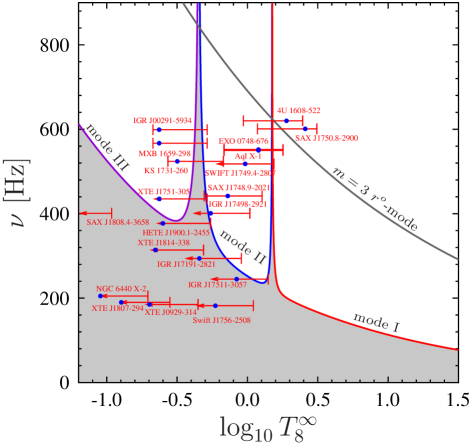
Figure 6: (color online) An example of the stability curves in case of two avoided crossings of $m=2$ oscillation modes of a superfluid NS. As in Fig. 4, the solid lines are plotted for modes I and II (red and blue online, respectively) experiencing an avoided crossing at $T^{\infty}=1.5\times 10^{8}$ K (the coupling parameter $s=0.001$). An additional solid line (violet online) corresponds to mode III, which exhibits an avoided crossing with the mode II at $T^{\infty}=4.5\times 10^{7}$ K. This avoided crossing is drawn for $s=0.01$. Other notations are the same as in Fig. 4.

The other sources with lower $T^{\infty}$ (e.g., IGR J00291-5934) can be explained in a similar manner. First, it is obvious that the temperature $T^{\infty}_{0}$ of the avoided crossing of modes I and II depends on the NS mass. Hence, if the masses of colder sources differ from those of the hotter ones, the avoided crossing of modes I and II can occur at a different $T^{\infty}_{0}$. In particular, it can be shifted to the region of lower temperatures, which are typical for these (rather cold) stars. Second, as it was shown in calculations of nonrotating NS oscillation spectra Gusakov and Andersson (2006); Kantor and Gusakov (2011); Chugunov and Gusakov (2011); Gusakov et al. (2013); Gualtieri et al. (2014), a normal mode can experience an avoided crossing with the superfluid modes more than once. To illustrate this idea, we demonstrate in Fig. 6 the instability curves in the case of two avoided crossings of oscillation modes. The first avoided crossing takes place at $T^{\infty}=4.5\times 10^{7}$ K between mode III (solid line marked “mode III” in the figure; violet online), which behaves as an $m=2$ $r^{o}$-mode at low $T^{\infty}$, and mode II (solid line; blue online). For this avoided crossing the coupling parameter was chosen to be $s=0.01$. The second avoided crossing of modes I and II is discussed above (see Fig. 5); it takes place at $T^{\infty}=1.5\times 10^{8}$ K. In this case mode II behaves as $m=2$ $r^{o}$-mode only at intermediate temperatures $6\times 10^{7}\ \mathrm{K}\lesssim T^{\infty}\lesssim 1.3\times 10^{8}$ K. At higher and at lower temperatures it transforms into superfluid modes, which are, generally, different. It is easy to demonstrate that, for low enough $T_{\mathrm{eq}}^{\infty}\lesssim 4\times 10^{7}$ K, the evolution track goes along the left (low-temperature) boundary of the first stability peak, corresponding to the avoided crossing of modes II and III [i.e., along the “mode III” line (violet online) in Fig. 6]. This stage is a direct analogue of the $C$–$D$ stage in Fig. 5, and a NS stays there for a long time. One sees that two avoided crossings are already sufficient to explain all the existing observations of frequencies and quiescent temperatures of NSs in LMXBs.

In summary, the sources IGR J00291-5934, MXB 1659-298, KS 1731-260, and XTE J1751-305 can be interpreted as moving along the instability curve of mode III (the curve which is violet online in the figure). This interpretation requires that their equilibrium temperature $T_{\mathrm{eq}}^{\infty}\lesssim 4\times 10^{7}$ K. The parameters of the objects IGR J17498-2921 and SAX J1748.9-2021 can be explained by accretion spin-up at $T^{\infty}=T_{\mathrm{eq}}^{\infty}\sim 5\times 10^{7}$ K, which takes place inside the stability region (an analogue of the $A$–$B$ stage in the scenarios discussed above). Finally, an explanation of the hottest stars 4U 1608-522, SAX J1750.8-2900, EXO 0748-676, Aql X-1, and SWIFT J1749.4-2807 remains the same as in the scenario with one avoided crossing (however, because of the additional avoided crossing the equilibrium temperature $T_{\mathrm{eq}}^{\infty}$ should comply with the condition $5\times 10^{7}\ \mathrm{K}\lesssim T_{\mathrm{eq}}^{\infty}\lesssim 1.4\times 10^{8}$ K for these sources). The rest of the stars lie in the stability region (even without accounting for the resonant coupling of modes), so they can be explained as being in the $A$–$B$ stage with the corresponding equilibrium temperature $T^{\infty}_{\rm eq}$ (see Sec. III.2).

Let us note that, to spin up the rapidly rotating sources up to the observed spin frequencies $\Omega$ during the time period shorter than the age of the Universe $t_{\mathrm{Un}}$, one needs quite a strong accretion torque $\dot{\Omega}_{\mathrm{acc}}^{\rm(crit)}\gtrsim\Omega/t_{\mathrm{Un}}\sim 3\times 10^{-7}$ s^-1 yr^-1, and hence quite a high accretion rate [$\dot{M}_{\rm crit}\gtrsim 10^{-11}M_{\odot}/\mathrm{yr}$ if one uses Eq. (21)]. Thus, to explain the low-temperature sources (those like MXB 1659-298) a rapid NS cooling may be required (e.g., with the open direct Urca process in the central regions of the star; see Ref. Yakovlev et al. (2001) and Sec. VII), which allows one to have a lower $T_{\mathrm{eq}}^{\infty}$ at higher ${\dot{M}}$. This can indicate that the coldest rapidly rotating NSs in LMXBs are more massive. An alternative explanation of these sources (not requiring an enhanced cooling) is also possible. It implies a more efficient accretion torque for these objects, that results in a large value of $\dot{\Omega}_{\mathrm{acc}}$ at a relatively small accretion rate ${\dot{M}}$. The last hypothesis agrees with the very low observational estimate $\dot{M}\approx 2.5\times 10^{-12}\,M_{\odot}/{\rm yr}\ll\dot{M}_{\rm crit}$ for the source IGR J00291-5934 (see Table 1), as well as with the results of Ref. Andersson et al. (2014), in which it is shown that the high spin-up rates observed for XTE J1751-305 and IGR J00291+5934 are not quite consistent with theoretical estimates. In Fig. 6 we have considered a situation in which an additional avoided crossing appears at lower $T^{\infty}$ than for modes I and II. It is also interesting to see how the additional avoided crossing affects the NS evolution if it appears at higher $T^{\infty}$. This possibility is studied in Appendix C, where it is shown that the four conclusions ($i$)–($iv$) stated above hold true even in this case.

VII Neutron star evolution after the end of accretion phase and production of millisecond pulsars

Thus, we demonstrate that the high spin frequencies of NSs in LMXBs can naturally be explained within our new scenario. But is this scenario compatible with the existence of millisecond pulsars (MSPs)? It is generally believed Alpar et al. (1982) that MSPs originate from LMXBs, in which accretion has ceased for some reason, for example, because of a binary system evolution Tauris (2011); Tauris and van den Heuvel (2006) or close encounter with some other star Ivanova et al. (2008). Let us consider the evolution of a NS with accretion switched off. A few alternatives are possible.

• Accretion ceases when a NS is in stage $A$–$B$ or in a similar stage with lower $T^{\infty}_{\rm eq}$.

  Then the star is stable and CFS instability does not affect its evolution. As a result, the NS cools down rapidly, keeping its spin frequency almost unchanged and eventually becomes a MSP. In this formation channel NS spin frequencies are limited by the instability curve. For realistic $T^{\infty}_{\mathrm{eq}}\;\raise 1.29167pt\hbox{$>$\kern-7.5pt\raise-4.73611pt\hbox{$\sim$}}\;4\times 10^{7}$ K this means that only MSPs with spin frequencies up to $\nu\lesssim 400$ Hz can be formed in this way (see Fig. 6). To form even faster MSPs, with $\nu$ up to $500$ Hz, one should assume that they had lower equilibrium temperatures ($T_{\rm eq}^{\infty}\sim 10^{7}$ K) in the $A$–$B$ stage. This is possible (see below), provided that these stars are massive enough so that strong neutrino emission processes (such as nucleon and/or hyperon direct Urca processes) are opened in their cores.

• Accretion ceases when a NS is climbing up the high-temperature peak in the $C$–$D$ stage (see Fig. 5).

  In that case a NS remains attached to the stability peak because its cooling would make the CFS instability stronger and heat the star up (the same situation as in the LMXB system with accretion; see Sec. VI). When accretion ceases, the equilibrium amplitude $\alpha^{({\rm eq})}_{\rm II}$ for mode II increases slightly [see Eq. (46) with $\dot{M}=0$]. Since in the absence of accretion $\dot{\Omega}_{\rm acc}=0$, NS spin frequency will gradually decrease as the rotation energy is carried away by gravitational waves and neutrinos. To get an impression about the typical times of climbing down, let us estimate the time $\Delta t_{DC}$ spent by a NS on the way from point $D$ to point $C$. Even for a very high $T^{\infty}=1.5\times 10^{8}$ K (and hence $L_{\rm cool}\approx 3.45\times 10^{34}$ erg s^-1), Eq. (47) with $\dot{\Omega}_{\rm acc}=0$ and $\dot{M}=0$ gives

  $$\Delta t_{DC}=\frac{\widetilde{J}\,M\,R^{2}\,(\Omega_{D}^{2}-\Omega_{C}^{2})}{4\,Q_{\rm II}\,L_{\rm cool}}\approx 1.5\times 10^{9}\,{\rm yr}.$$ (51)

  Such a long time indicates that the probability to observe a rapidly rotating nonaccreting NS climbing down the peak is not small. It is easy to demonstrate that, due to magnetodipole losses only [see Eq. (50)], a star would spin down during the same period of time if it had the dipolar magnetic field at the poles $B\approx 7\times 10^{8}$ G.

  In Refs. Gusakov et al. (2014); Chugunov et al. (2014) it is argued that these nonaccreting NSs, heated by the CFS instability, form a specific new class of NSs. These references propose to call them “HOFNARs” (from HOt and Fast Non-Accreting Rotators) or “hot widows” (in analogy with the “black widow” pulsars), and suggest that a number of sources that are tentatively identified as quiescent LMXB candidates may in fact be such objects.

  Could “hot widows”/HOFNARs, descending the high-temperature peak, be associated with MSPs? Most probably not, because these objects are very hot, with effective surface temperature $T_{\rm eff}^{\infty}\sim 10^{6}$ K (and internal temperature $T^{\infty}\sim 10^{8}$ K), while it is customary to assume that MSPs are much colder (only their hot spots can reach the values $\sim 10^{6}$ K). The high temperature of “hot widows”/HOFNARs explains, most likely, the fact that these objects do not show radio pulsar activity: The magnetic field in hot NSs decays much faster (see, e.g., Refs. Urpin and Konenkov (2008); Chugunov et al. (2014)). The detailed analysis of this possible new class of NSs from both theoretical and observational points of view is presented in Ref. Chugunov et al. (2014).

• Accretion ceases when a NS is climbing up the low-temperature peak (like the left peak in Fig. 6 or a similar peak at lower temperature).

  The subsequent evolution of a NS is then quite similar to that in the case of the high-temperature peak. The star becomes a “hot widow”/HOFNAR; the only difference is that now its temperature is noticeably smaller. As a consequence, such star can maintain its magnetic field and be, at the same time, a MSP. Therefore, MSPs with spin frequencies $\nu\gtrsim(400$–$500)$ Hz (including the most rapidly rotating pulsar PSR J1748-2446ad with $\nu=716$ Hz) are interpreted by us as NSs, climbing down the low-temperature stability peak.

  Here it is pertinent to ask the following question: What is the minimal possible temperature $T_{0}^{\infty}$ of the stability peak, at which a NS still can find itself there? Obviously, for that to be possible, the equilibrium internal temperature $T_{\rm eq}^{\infty}$ of the star should be smaller than $T_{0}^{\infty}$. This temperature is found from the condition $L_{\rm cool}=K_{\rm n}\dot{M}c^{2}$. It can be shown that even for $\dot{M}=\dot{M}_{\rm crit}$ and completely unsuppressed nucleon direct Urca process (which is quite unrealistic) $T_{\rm eq}^{\infty}\;\raise 1.29167pt\hbox{$>$\kern-7.5pt\raise-4.73611pt\hbox{$\sim$}}\;6\times 10^{6}$ K, which corresponds to the effective surface temperature $T_{\rm eff}^{\infty}\;\raise 1.29167pt\hbox{$>$\kern-7.5pt\raise-4.73611pt\hbox{$\sim$}}\;3\times 10^{5}$ K (for $P/g=10^{9}$ g cm^-2, see Sec. III.1). In a more realistic case, when we have a completely unsuppressed direct Urca process with $\Lambda$ hyperons ($\Lambda\rightarrow p+e+\bar{\nu}_{e}$; see, e.g., Ref. Yakovlev et al. (2001)), operating in the inner half of the NS core ($r\leq R/2$), one obtains $T_{\rm eq}^{\infty}\sim 1.3\times 10^{7}$ K, which corresponds to $T_{\rm eff}^{\infty}\sim 4.6\times 10^{5}$ K.

  One sees that both estimates give rather large values of minimal equilibrium temperature. As a consequence, the effective surface temperatures of MSPs with the spin frequencies $\nu\gtrsim 400$–$500$ Hz, which, according to our scenario, are climbing down the low-temperature stability peak, cannot be lower than $T_{\rm eff}^{\infty}\sim(3$–$5)\times 10^{5}$ K. It is important to note that this conclusion can change in a more complicated scenario which accounts for a possible resonance interaction of the core $r$-modes with elastic modes of the crust Levin and Ushomirsky (2001); Yoshida and Lee (2001); Glampedakis and Andersson (2006a). In such scenario a NS can leave, under certain conditions, the stability peak and cool down to very low temperatures (see Appendix D). Note also that accounting for the interaction of $r$-modes with the crust modes allows one to explain cold MSPs with $\nu\gtrsim(400$–$500)$ Hz without invoking powerful neutrino emission processes (such as the direct Urca process) in the NS core.

In conclusion, the proposed scenario can explain the formation of MSPs, including the most rapidly rotating pulsars. It also predicts the existence of a new class of hot and rapidly rotating NSs – “hot widows”/HOFNARs (see Ref. Chugunov et al. (2014) for details).

VIII Conclusions

We demonstrate that the key role in the evolution of NSs in LMXBs is played by the resonance interaction of the normal $m=2$ oscillation $r$-mode ($r^{o}$-mode) and the superfluid inertial modes ($i^{s}$-modes). This result allows us to formulate a scenario that explains observations of rapidly rotating warm NSs in LMXBs (Sec. VI) and predicts the existence of a new class of nonaccreting NSs which we propose to call “hot widows” or HOFNARs (see Sec. VII and Ref. Chugunov et al. (2014) for more details). This scenario is in agreement with the existence of MSPs (Sec. VII and Appendix D), predicting that some of them [especially, most rapidly rotating MSPs with $\nu\gtrsim(400$–$500)$ Hz] can be rather hot, with the effective surface temperatures $T_{\rm eff}^{\infty}\;\raise 1.29167pt\hbox{$>$\kern-7.5pt\raise-4.73611pt\hbox{$\sim$}}\;(3$–$5)\times 10^{5}$ K. A more detailed analysis of our scenario in application to MSPs will be reported elsewhere.

The conclusion about the resonance interaction of $i^{s}$- and $r^{o}$-modes is based on the following facts:

$1.$ Detailed calculations Gusakov and Andersson (2006); Gusakov and Kantor (2011); Kantor and Gusakov (2011); Chugunov and Gusakov (2011); Gusakov et al. (2013); Gualtieri et al. (2014) of the oscillation spectra of nonrotating superfluid NSs at finite temperatures $T^{\infty}$ reveal that ($i$) The frequencies of the superfluid modes essentially depend on $T^{\infty}$, while those of the normal modes are almost insensitive to a temperature variation. ($ii$) If, at some $T^{\infty}$, the frequencies $\omega$ of two arbitrary (but with the same “quantum” number $m$) superfluid and normal modes become equal, they start to interact resonantly. As a result of such interaction, the superfluid mode turns into the normal one and vice versa; that is, an avoided crossing of modes is formed in the $\omega-T^{\infty}$ plane. ($iii$) Far from the avoided crossings superfluid and normal modes are almost noninteracting and are described by the two weakly coupled systems of equations.

$2.$ According to computations of Lee and Yoshida Lee and Yoshida (2003); Yoshida and Lee (2003a) performed in the $T^{\infty}=0$ approximation, the frequencies of $i^{s}$-modes are sensitive to a variation of the so-called entrainment parameter $\widetilde{\eta}$ (see Sec. IV.1). In particular, at some specific values of $\widetilde{\eta}$ avoided crossings of superfluid and normal oscillation modes are observed (see also Sec. IV.2).

$3.$ An account for finite $T^{\infty}$ leads to a temperature dependence of a number of parameters of superfluid hydrodynamics (including $\widetilde{\eta}$).

Items $2$ and $3$ give us a ground to assume that the results formulated in item $1$ in application to nonrotating NSs remain valid for rotating NSs as well. Hence, the frequencies of $i^{s}$-modes should also depend on $T^{\infty}$. This means, in particular, that avoided crossings between the $m=2$ $r^{o}$-mode and $i^{s}$-modes should be formed at some values of $T^{\infty}$ (see, e.g., Fig. 3). When passing through an avoided crossing, the $i^{s}$-mode transforms into the $m=2$ $r^{o}$-mode, while the $m=2$ $r^{o}$-mode becomes the $i^{s}$-mode. During such a transformation the eigenfunctions of the $m=2$ $r^{o}$-mode mix intensively with those of the $i^{s}$-mode. This leads to the enhancement of $r^{o}$-mode damping due to mutual friction (see Sec. IV.2). In the $\nu-T^{\infty}$ plane, this effect is manifested by the appearance of a sharp “stability peak” over the standard (usually considered) stability region of fast rotating NSs (see Sec. V.1 and Fig. 4; the stability region is filled with grey there).

An analysis of evolution of a NS in LMXB taking into account the stability peak shows that the star spends a significant amount of time climbing the left side of this peak in the region, which has been previously thought to be unstable with respect to excitation of $r$-modes. To keep on the peak, the average oscillation amplitude adjusts itself so that the star heating due to dissipation of oscillations is compensated by neutrino cooling. Under such circumstances, a spin-down due to gravitational wave emission can be insufficient to oppose the accretion torque on the star. This leads to a gradual increasing of the NS spin frequency as it slowly climbs up the peak (see Sec. VI for details).

If spin-up is not terminated by the magnetic field (see footnote 20), the star reaches the instability curve for the $m=3$ oscillation $r^{o}$-mode, which is the next unstable mode in normal NSs after the $m=2$ $r^{o}$-mode. As a result, the star jumps off the peak and shortly returns to the stability region (see Sec. VI). Thus, the real limit on the spin frequency of NSs is set by the instability curve for the octupole $m=3$ $r^{o}$-mode. This result allows us to explain the fast rotation of NSs in LMXBs within the minimal assumptions about the properties of superdense matter. Moreover, this result agrees with the predicted Chakrabarty et al. (2003); Chakrabarty (2008) abrupt cutoff above $\sim 730$ Hz of the spin frequency distribution of accreting millisecond X-ray pulsars. Furthermore, because $\dot{\Omega}\approx\dot{\Omega}_{\rm acc}$ in the $A$–$B$ and $C$–$D$ stages, our scenario predicts the frequency distribution to be almost constant at $200$–$600$ Hz, in agreement with observations (see, e.g., Fig. 5 of Ref. Patruno (2010)).

It is important to emphasize that our scenario is almost insensitive to an actual choice of the parameters regulating the resonance interaction between the modes (resonance temperatures and width of the peaks; see Secs. IV and V) and does not require any nonrealistic enhancement of the kinetic coefficients and/or additional exotic damping mechanisms.

Obviously, the new approach to the evolution of rapidly rotating NSs and interpretation of their observations, suggested in the present paper, needs further development and refinement. In particular, one needs to perform detailed calculations in order to confirm the presence of avoided crossings in the oscillation spectra of warm superfluid rotating NSs, and to study how the resonance interaction of modes affects the oscillation damping times. We expect that the corresponding resonance temperatures will depend on the NS mass and on the parameters of superfluidity. A detailed analysis of the effect of various damping processes (such as, e.g., Ekman layer dissipation Bildsten and Ushomirsky (2000); Rieutord (2001a, b); Andersson and Kokkotas (2001); Glampedakis and Andersson (2006b)) on the instability curve of the octupole $m=3$ $r^{o}$-mode will place further restrictions on the spin frequencies of NSs.

If our scenario is correct, then the observed temperatures of the most rapidly rotating NSs must coincide with the temperatures $T^{\infty}_{0}$, at which avoided crossings occur between the $m=2$ $r^{o}$-mode and the superfluid $i^{s}$-modes. Comparison of these temperatures $T^{\infty}_{0}$ with the results of (still not available) theoretical calculations can impose stringent constraints on the properties of superdense matter and parameters of superfluidity. Clearly, a direct observational test of our scenario is a very important task which we plan to address in the nearest future. In particular, we plan to study in detail the modulation of the NS spin frequency, appearing when the star moves along the stability peak (see Sec. VI), and to examine whether this effect can be confirmed observationally.

Appendix A The approximations for neutrino luminosity and heat capacity

The neutrino luminosity $L_{\rm cool}$ and total heat capacity $C_{\rm tot}$ of a NS with the mass $M=1.4M_{\odot}$ are calculated with the relativistic cooling code, described in detail in Refs. Gusakov et al. (2004); Gusakov et al. (2005a); Yakovlev and Pethick (2004). We use essentially the same microphysics input as in Ref. Gusakov et al. (2004). In particular, we employ the parametrization Heiselberg and Hjorth-Jensen (1999) of APR EOS Akmal et al. (1998). The results of our calculations of $L_{\rm cool}$ and $C_{\rm tot}$ are roughly fitted by the following formulas

$$L_{\rm cool} = 7\times 10^{30}\left(T^{\infty}_{8}\right)^{8}\,\left\{\sqrt{1.25\,T^{\infty}_{8}}+140\,\exp\left(-\frac{30}{T_{8}^{\infty}}\right)\right.$$ (52)

$$+ \left.3\times 10^{4}\,\exp\left[-\left(\log_{10}T_{8}^{\infty}+0.5\right)^{2}/0.3^{2}\right]\right\}\,\mathrm{erg\,s}^{-1},$$

$$C_{\rm tot} = 2.1\times 10^{37}\,T^{\infty}_{8}\,\left(1+\frac{6}{(0.18/T^{\infty}_{8})^{3.6}+1}\right)\,{\rm erg}\,{\rm K}^{-1}.$$ (53)

The last term in the expression for $L_{\rm cool}$ corresponds to the enhancement of the neutrino luminosity due to neutron Cooper pairing.

Appendix B NS evolution in the absence of resonant interaction with superfluid modes

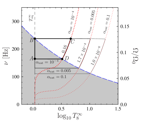
Figure 7: (color online) Analogous to Fig. 2, but in a larger scale. The evolution of the spin frequency $\nu$ and temperature $T^{\infty}_{8}$ is shown for a NS in LMXB in the absence of resonant interaction of modes. The corresponding tracks are shown by solid lines (black online; thick, medium, and thin lines are for $\alpha_{\mathrm{sat}}=10^{-4}$, $0.005$, and $0.1$, respectively). The numbers near the lines indicate the fraction of time the star spends in the instability region (this fraction is calculated without accounting for the time $\Delta t_{\rm torq}\approx 4500$ yr, during which the star is located at point $B$). The stability region of the $m=2$ $r^{o}$-mode is filled with grey; its boundary is shown by a thick dashed line (blue online). Vertical dashed line shows the equilibrium stellar temperature $T_{\mathrm{eq}}^{\infty}$. The dotted curves are plotted assuming that the neutrino cooling exactly balances the stellar heating due to nonlinear dissipation of the saturated $m=2$ $r^{o}$-mode (the Cooling=Heating curves). See text for details.

Let us analyze the evolution of a NS in LMXB in the absence of resonant interaction of the normal $r^{o}$-mode with superfluid modes. A similar scenario was proposed, for the first time, in Ref. Levin (1999) (see also Ref. Heyl (2002)). Here we reconsider it, employing the physics input, described in Sec. II, and perform a number of useful estimates, supplementing the consideration of Sec. III.2. Figure 7 presents the stellar spin frequency $\nu$ as a function of the internal redshifted temperature $T^{\infty}$. The thick solid line shows the cyclic evolution track of the NS $A$–$B$–$C$–$D$–$A$ for the saturation amplitude of the $r^{o}$-mode $\alpha_{\rm sat}=10^{-4}$. The medium and thin solid lines show similar tracks for $\alpha_{\rm sat}=5\times 10^{-3}$ and $\alpha_{\rm sat}=10^{-1}$, respectively.

The instability curve for the quadrupole $m=2$ $r^{o}$-mode, given by the condition $1/\tau_{\rm GR}+1/\tau_{\rm Diss}=0$, is shown by a thick dashed line (blue online). In the region over the curve one has $1/\tau_{\rm GR}+1/\tau_{\rm Diss}<0$ and, as follows from Eq. (19), the star is unstable with respect to excitation of the $r^{o}$-mode ($d\alpha/dt>0$). In the figure the stability region for the $m=2$ $r^{o}$-mode is filled with grey.

Let us discuss in more detail the stellar evolution along the track $A$–$B$–$C$–$D$–$A$.

($i$) Stage $A$–$B$.

The star has initial equilibrium temperature $T_{A}^{\infty}=T_{\rm eq}^{\infty}\approx 1.078\times 10^{8}$ K (see Sec. III.2), the amplitude of the $r^{o}$-mode $\alpha=0$, and the spin frequency $\nu_{A}\approx 164$ Hz ($\Omega_{A}=2\pi\nu_{A}\approx 1030$ s^-1). The stellar spin frequency grows linearly due to accretion of matter onto the NS according to Eq. (20) with $\alpha=0$. The stellar temperature $T^{\infty}$ remains unchanged. The star reaches the boundary of the stability region at point $B$. In this point $\nu_{B}\approx 238$ Hz ($\Omega_{B}\approx 1495$ s^-1), so that the time spent by the star in stage $A$–$B$ equals $\Delta t_{AB}=(\Omega_{B}-\Omega_{A})/\dot{\Omega}_{\rm acc}\approx 4\times 10^{7}$ yr.

($ii$) The stage $B$–$C$.

At point $B$, the star is located on the instability curve of the $m=2$ $r^{o}$-mode. Further increasing of the stellar spin frequency makes it unstable. However, if the $r^{o}$-mode amplitude is strictly zero, then, as follows from Eq. (19), $d\alpha/dt$ remains to be zero even in the instability region. In reality, of course, any fluctuation of the amplitude $\alpha$ (for instance, the thermal fluctuation or a fluctuation related to accretion onto a NS) will lead to instability growth. In numerical calculations we modeled this effect by specifying the initial condition $\alpha_{B}=10^{-30}$ for the oscillation amplitude at point $B$. Naturally, the subsequent NS evolution is not sensitive to the actual value of the initial amplitude.

Becoming unstable, the amplitude of $m=2$ $r^{o}$-mode grows rapidly, so that after $\Delta t_{\rm torq}\approx 4500$ yr the torque acting on the NS due to $r^{o}$-mode dissipation becomes equal to the accretion torque [$d\Omega/dt=0$; see Eq. (20)]. This happens at $\alpha_{0}\approx 1.8\times 10^{-5}$. Approximately $4$ yr later the $r^{o}$-mode reaches saturation ($\alpha=\alpha_{\rm sat}=10^{-4}$). During these evolution phases $\Omega$ and $T^{\infty}$ almost do not change. The spin frequency $\Omega$ does not change because a typical time scale of its variation is much greater than $\Delta t_{\rm torq}$ (see below). The temperature $T^{\infty}$ does not change, because its typical time scale is $\propto\alpha^{-2}$ [see Eqs. (16) and (17)] and is also much greater than $\Delta t_{\rm torq}$ most of the time.

Using the fact that $\Omega$ and $T^{\infty}$ are almost constant, $\alpha_{0}$ can be derived from Eq. (20) if we fix $\Omega=\Omega_{B}$ and $T^{\infty}=T^{\infty}_{\rm eq}$ and make its left-hand side vanish,

$$\alpha_{0}=\sqrt{\frac{\dot{\Omega}_{\rm acc}\,\tau_{\rm Diss}(T^{\infty}_{\rm eq})}{2\,Q\,\Omega_{B}}}\approx 1.8\times 10^{-5}.$$ (54)

The time $\Delta t_{\rm torq}$ can also be roughly estimated if one keeps in mind that, in the initial stage of the instability, the amplitude $\alpha$ stays small. In that case, the first term in the right-hand side of Eq. (20) can be neglected, so that one obtains

$$\Omega-\Omega_{B}\approx\dot{\Omega}_{\rm acc}(t-t_{B}).$$ (55)

Using this equation and expanding into Taylor series the right-hand side of Eq. (19) around point $B$ (at fixed $T^{\infty}=T^{\infty}_{\rm eq}$), one gets

$$\frac{d\alpha}{dt}\approx\alpha\,\,\frac{|\tau^{\prime}_{\rm GR}(\Omega_{B})|}{\tau_{\rm GR}^{2}(\Omega_{B})}\,\,\dot{\Omega}_{\rm acc}\,(t-t_{B}),$$ (56)

or, after trivial integration,

$$\alpha=\alpha_{B}\,{\rm e}^{(t-t_{B})^{2}/\tau_{\alpha}^{2}},\quad\quad{\rm where}\quad\quad\tau_{\alpha}=\sqrt{\frac{2\tau_{\rm GR}^{2}(\Omega_{B})}{|\tau^{\prime}_{\rm GR}(\Omega_{B})|\,\dot{\Omega}_{\rm acc}}}\approx 600\,{\rm yr}.$$ (57)

Substituting now $\alpha=\alpha_{0}$ into this equation, one finds

$$\Delta t_{\rm torq}\approx\tau_{\alpha}\,\sqrt{\ln\left(\frac{\alpha_{0}}{\alpha_{B}}\right)}\approx 4600\,{\rm yr}.$$ (58)

This result is just a little bit larger than the exact value $\Delta t_{\rm torq}\approx 4500$ yr. As shown in Sec. II, the NS evolution with the saturated $r^{o}$-mode is governed by the simpler equations. In particular, instead of Eq. (20) one will have

$$\frac{d\Omega}{dt}=\frac{2\,Q\,\alpha_{\rm sat}^{2}\,\Omega}{\tau_{\rm GR}}+\dot{\Omega}_{\rm acc},$$ (59)

which can be integrated independently. Neglecting the term $\dot{\Omega}_{\rm acc}$, which is small in our case [$\dot{\Omega}_{\rm acc}$ becomes comparable to the first term in the right-hand side of Eq. (59) at a small $\Omega\approx 915$ s^-1 ($\nu\approx 146$ Hz), and can be omitted for a rough estimate], we get

$$\Omega=\frac{\Omega_{B}}{(1+t/\tau_{\Omega})^{1/6}},\quad{\rm with}\quad\tau_{\Omega}=-\frac{1}{12}\,\,\frac{\tau_{\rm GR}(\Omega_{B})}{Q\,\alpha_{\rm sat}^{2}}\approx\frac{3\times 10^{-8}}{\alpha_{\rm sat}^{2}}\,\left(\frac{\Omega_{0}}{\Omega_{B}}\right)^{6}\,{\rm yr}\approx 7\times 10^{5}\,{\rm yr},$$ (60)

where the time is counted from the moment when the $r^{o}$-mode reaches saturation. In practice, this formula describes the $\Omega(t)$ dependence on the whole interval $B$–$C$–$D$ sufficiently well.

Let us now estimate the time $\Delta t_{T}$ required to heat up the star from the moment of $r^{o}$-mode saturation to point $C$. Point $C$ lies on the Cooling=Heating curve, given by the condition

$$-\frac{\widetilde{J}MR^{2}\Omega^{2}\alpha_{\rm sat}^{2}}{\tau_{\rm GR}}-L_{\rm cool}+K_{\rm n}\dot{M}c^{2}=0,$$ (61)

which means that at this curve the stellar heating due to dissipation of the saturated $r^{o}$-mode is exactly compensated by the neutrino cooling. After reaching the curve, the star moves along it, until it enters the stability region. As we will see from the estimate, $\Delta t_{T}$ is much smaller than $\tau_{\Omega}$; thus, in the further derivation one can set $\Omega=\Omega_{B}$ ($=\Omega_{C}$) in Eq. (16). Bearing in mind that the mode is saturated (that is, $\alpha=\alpha_{\rm sat}$ and instead of $\tau_{\rm Diss}$ one should write $-\tau_{\rm GR}$), Eq. (16) can be rewritten as

$$C_{\rm tot}\frac{dT^{\infty}}{dt}=-\frac{\widetilde{J}MR^{2}\Omega_{B}^{2}\alpha_{\rm sat}^{2}}{\tau_{\rm GR}}-L_{\rm cool}+K_{\rm n}\dot{M}c^{2}.$$ (62)

Making the left-hand side of this equation vanish, one finds the stellar temperature at point $C$, $T^{\infty}_{C}\approx 4.6\times 10^{8}$ K. Equation (62) can now be integrated in quadratures. However (since we are only interested in the order-of-magnitude estimate for $\Delta t_{T}$), we additionally simplify it by neglecting the last two terms in the right-hand side of this equation. In addition, we make use of the fact that in the range of temperatures under consideration the heat capacity $C_{\rm tot}\approx\gamma T^{\infty}$, where $\gamma\approx 1.5\times 10^{30}$ erg K^-2. Integrating now Eq. (62), we obtain

$$\Delta t_{T}=\frac{\gamma\,\tau_{\rm GR}\,(T_{\rm eq}^{\infty\,2}-T_{C}^{\infty\,2})}{2\widetilde{J}\,M\,R^{2}\,\Omega_{B}^{2}\,\alpha_{\rm sat}^{2}}\approx 1200\,{\rm yr}.$$ (63)

Because we ignored the star luminosity $L_{\mathrm{cool}}$ in Eq. (62), our rough estimate is smaller than the real time $\Delta t_{T}\approx 3300$ yr. In reality, $L_{\mathrm{cool}}$ becomes important and slows down the NS heating only in the very vicinity of the curve Cooling=Heating. According to our estimate, for the first $\sim 1300$ yr the star rapidly heats up and reaches the boundary of the circle, shown as point $C$ in the figure. During the subsequent $\sim 2000$ yr the star heating proceeds very slowly and its position in Fig. 7 almost does not change. As we expected, $\Delta t_{T}\ll\tau_{\Omega}$.

($iii$) Stage $C$–$D$.

This is the longest stage in the instability region. During it the star moves along the Cooling=Heating curve. The time spent on the horizontal stage $B$–$C$ is several orders of magnitude smaller. The Cooling=Heating curve crosses the instability curve at point $D$, $\Omega_{D}\approx\Omega_{A}$. The traveling time along $C$–$D$ can be easily estimated from Eq. (60),

$$\Delta t_{CD}\approx\tau_{\Omega}\,\left(\frac{\Omega_{C}^{6}}{\Omega_{D}^{6}}-1\right)\approx\frac{3\times 10^{-8}}{\alpha_{\rm sat}^{2}}\left(\frac{\Omega_{0}^{6}}{\Omega_{D}^{6}}-\frac{\Omega_{0}^{6}}{\Omega_{C}^{6}}\right)\,{\rm yr}\approx 6\times 10^{6}\,{\rm yr}.$$ (64)

The exact calculation shows that $\Delta t_{CD}\approx 8\times 10^{6}$ yr. The discrepancy is due to neglect of the term $\dot{\Omega}_{\rm acc}$ in the derivation of Eq. (60).

($iv$) Stage $D$–$A$.

Just after the star reaches the stability region, the amplitude of $r^{o}$-mode rapidly (during $\sim 400$ yr) decreases to negligible values; then the star cools down to the temperature $T_{\rm eq}^{\infty}$ (point $A$). The cooling takes $\sim 10^{5}$ yr, and after that the cycle repeats.

The main conclusion that can be drawn from the discussion of the evolution tracks is as follows: in the stability region the star spends most of the time in stage $A$–$B$, while in the instability region – in the stage $C$–$D$. The ratio of the time spent in the instability region (without accounting for the time $\Delta t_{\rm torq}\approx 4500$ yr, during which the star “sits” at point $B$; see Fig. 7) to the period of the cycle equals $k\approx 0.16$ for the model with $\alpha_{\rm sat}=10^{-4}$. This ratio drops rapidly with increasing $\alpha_{\rm sat}$ Heyl (2002), because the typical time $\tau_{\Omega}$ of $\Omega$ variation during the $C$–$D$ stage is $\tau_{\Omega}\propto\alpha_{\rm sat}^{-2}$; see Eq. (60). For $\alpha_{\rm sat}=5\times 10^{-3}$ we have $k\approx 1.7\times 10^{-4}$, whereas for $\alpha_{\rm sat}=10^{-1}$ we obtain $k\approx 10^{-6}$. Let us note that, since in the saturation regime $W_{\rm Diss}\propto\alpha_{\rm sat}^{2}$, the higher $\alpha_{\rm sat}$ is, the farther the NS gets into the region of high temperatures (the more horizontally elongated is the track $A$–$B$–$C$–$D$–$A$; see Fig. 7).

Appendix C NS evolution in the case of two avoided crossings of oscillation modes

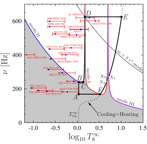
Figure 8: (color online) Similar to Fig. 5, but with additional avoided crossing of modes I and III at $T^{\infty}=5\times 10^{8}$ K. An instability curve for mode III is shown by the correspondingly marked solid line (violet online); the coupling parameter parametrizing interaction between modes I and III is $s=0.001$. The evolution track $A$–$B$–$C$–$D$–$E$–$X_{1}$–$X_{2}$–$X_{3}$–$F$–$A$ of a star is shown by the solid line. Other notations (and input parameters) coincide with those in Fig. 5.

Assume that, besides the avoided crossing of modes I and II, there is one more avoided crossing of modes I and III at $T^{\infty}=5\times 10^{8}$ K such that mode III becomes the $m=2$ $r^{o}$-mode at $T^{\infty}>5\times 10^{8}$ K (see Fig. 8). The thick solid line in Fig. 8 shows the typical evolution track $A$–$B$–$C$–$D$–$E$–$X_{1}$–$X_{2}$–$X_{3}$–$F$–$A$ of a NS in this case. The main difference between this track and the one discussed in Sec. VI (see Fig. 5) is stage $X_{1}$–$X_{2}$–$X_{3}$, in which the star evolves in the region of avoided crossing of modes I and III.

Let us discuss this stage in more detail. At point $X_{1}$, the only excited mode is the oscillation mode III, which is saturated (i.e., its amplitude equals $10^{-4}$). At stage $X_{1}$–$X_{2}$, the star enters the stability region, where the amplitude of mode III rapidly vanishes, and the star cools down to point $X_{2}$ during $\sim 130$ yr. At point $X_{2}$, the star becomes unstable with respect to excitation of mode I; similar to the case of mode II at stage $C$–$D$ (see Fig. 8), its equilibrium amplitude $\alpha^{\rm(eq)}_{\mathrm{I}}$ is then defined by the thermal equilibrium condition (46). Since stage $X_{2}$–$X_{3}$ is close to the curve Cooling=Heating, intensive heating is required to maintain the temperature, and mode I appears to be close to saturation. Such a high oscillation amplitude means that the spin-down of the NS due to viscous dissipation of mode I will dominate the accretion torque [see Eq. (47)]. As a result, the stellar spin frequency will decrease. Finally, in $4.6\times 10^{5}$ yr after leaving point $X_{2}$ (this time constitutes $\sim 0.16\%$ of the full period of the cycle), the star again reaches the Cooling=Heating curve at point $X_{3}$. To continue spinning down along the instability curve of mode I, it needs a more intensive heating than the saturated mode can provide. Thus, the further evolution of the star (stage $X_{3}$–$F$) goes along the Cooling=Heating curve, as in the scenario shown in Fig. 5.

We arrive at the conclusion, that the existence of additional avoided crossings of oscillation modes does not affect noticeably the scenario, proposed in Sec. VI, and does not change the main results of the paper.

Appendix D NS evolution in the presence of a resonance interaction of the normal r-mode with the crustal toroidal modes

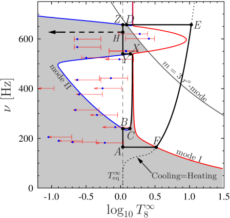
Figure 9: (color online) The same as Fig. 5, but with resonance interaction of the $r$-mode and a torsional crustal mode at 600 Hz taken into account. The evolution track $A$–$B$–$C$–$X$–$Y$–$Z$–$D$–$E$–$F$–$A$ of a star is shown by the thick solid line. Horizontal dashes show NS evolution for the case when accretion ceases at point $H$. The vertical dashed line indicates $T^{\infty}_{\rm eq}$.

The presence of elastic crust may substantially modify the oscillation spectrum of rotating NSs. Numerous calculations (see, e.g., Refs. Lee and Strohmayer (1996); Levin and Ushomirsky (2001); Yoshida and Lee (2001); Glampedakis and Andersson (2006a)) show that the $r$-mode in that case experiences avoided crossings with torsional crustal modes at some spin frequencies. An important feature of $r$-mode eigenfunctions near these frequencies is amplified relative velocity (slippage) between the elastic crust and liquid core. This amplification leads to an enhanced damping in the Ekman layer Levin and Ushomirsky (2001) near the avoided crossing that could modify the instability windows Levin and Ushomirsky (2001); Ho et al. (2011). In Fig. 9 we show a possible example of such a modified instability window. For illustration, we assume that there is only one avoided crossing of the normal $r$-mode and a superfluid inertial mode (see Fig. 5). In addition, we assume that the normal ($m=2$) $r$-mode experiences a resonant interaction with the torsional crustal mode at a rotation frequency $\nu_{\rm crust}=600\,\rm Hz$ Levin and Ushomirsky (2001); Ho et al. (2011). The resulting enhanced dissipation in the Ekman layer is modeled, in a simplified manner, by introducing an additional frequency-dependent term in the expression for the total inverse damping time scale $1/\tau_{\rm Diss}^{\rm norm}$ of the normal $r$-mode,

$$\frac{1}{\tau_{\rm Ek}^{\rm norm}}=\frac{0.08\,\rm s^{-1}}{(T^{\infty}_{8})^{2}}\,{\rm exp}\left[-1133\left(\frac{\nu-\nu_{\rm crust}}{1\,\rm kHz}\right)^{2}\right],$$ (65)

so that now $1/\tau_{\rm Diss}^{\rm norm}=1/\tau_{\rm S}^{\rm norm}+1/\tau_{\rm MF}^{\rm norm}+1/\tau_{\rm Ek}^{\rm norm}$ (while the corresponding inverse damping time scale $1/\tau_{\rm Diss}^{\rm sfl}$ for the superfluid mode is kept unchanged). The functional dependence and numerical values in Eq. (65) are purely illustrative. This additional dissipation leads to the appearance of the stability region at spin frequencies close to $\nu_{\rm crust}$ (see the filled grey region in Fig. 9) and modifies the evolutionary track of a NS, shown by the thick solid line. Stages $A$–$B$–$C$ are the same as in Fig. 5. From point $C$ a star climbs up the left edge of the stability peak until it reaches point $X$, where ongoing accretion brings it inside the stability region. The next stage $X$–$Y$ is similar to stage $F$–$A$: In the stability region, the $r$-mode dies out and the star cools down to $T_{\rm eq}^{\infty}$ (point $Y$). Then it spins up slowly in the stability region (like in the $A$–$B$ stage). At point $Z$, the star becomes unstable with respect to the $m=2$ $r$-mode and starts to heat up rapidly. At point $D$ it becomes, in addition, unstable with respect to the $m=3$ $r$-mode. The subsequent stages $D$–$E$–$F$–$A$ are analogous to those shown in Fig. 5. Note that, if accretion ceases at the stage $Y$–$Z$ (e.g., at point $H$), then the star will cool down (see the thick arrowed dashed line) and can become a very cold MSP with $\nu\;\raise 1.29167pt\hbox{$>$\kern-7.5pt\raise-4.73611pt\hbox{$\sim$}}\;500$ Hz.

References

- Haensel et al. (2007) P. Haensel, A. Y. Potekhin, and D. G. Yakovlev, Neutron Stars 1 : Equation of State and Structure (Springer, New York, 2007).
- Hessels et al. (2006) J. W. T. Hessels, S. M. Ransom, I. H. Stairs, P. C. C. Freire, V. M. Kaspi, and F. Camilo, Science 311, 1901 (2006), eprint arXiv:astro-ph/0601337.
- Unno et al. (1989) W. Unno, Y. Osaki, H. Ando, H. Saio, and H. Shibahashi, Nonradial oscillations of stars (University of Tokyo Press, Tokyo, 1989).
- Andersson and Kokkotas (2001) N. Andersson and K. D. Kokkotas, Int. J. Mod. Phys. D 10, 381 (2001), eprint arXiv:gr-qc/0010102.
- Andersson (1998) N. Andersson, Astrophys. J. 502, 708 (1998), eprint arXiv:gr-qc/9706075.
- Friedman and Morsink (1998) J. L. Friedman and S. M. Morsink, Astrophys. J. 502, 714 (1998), eprint arXiv:gr-qc/9706073.
- Patruno (2010) A. Patruno, Astrophys. J. 722, 909 (2010), eprint arXiv:1006.0815.
- Patruno and Watts (2012) A. Patruno and A. L. Watts, ArXiv e-prints (2012), eprint arXiv:1206.2727.
- Ho et al. (2011) W. C. G. Ho, N. Andersson, and B. Haskell, Physical Review Letters 107, 101101 (2011), eprint arXiv:1107.5064.
- Haskell et al. (2012) B. Haskell, N. Degenaar, and W. C. G. Ho, Mon. Not. R. Astron. Soc. 424, 93 (2012), eprint arXiv:1201.2101.
- Mahmoodifar and Strohmayer (2013) S. Mahmoodifar and T. Strohmayer, Astrophys. J. 773, 140 (2013), eprint arXiv:1302.1204.
- Levin (1999) Y. Levin, Astrophys. J. 517, 328 (1999), eprint arXiv:astro-ph/9810471.
- Heyl (2002) J. S. Heyl, Astrophys. J. Lett. 574, L57 (2002).
- Rutledge et al. (1999) R. E. Rutledge, L. Bildsten, E. F. Brown, G. G. Pavlov, and V. E. Zavlin, Astrophys. J. 514, 945 (1999), eprint arXiv:astro-ph/9810288.
- Heinke et al. (2007) C. O. Heinke, P. G. Jonker, R. Wijnands, and R. E. Taam, Astrophys. J. 660, 1424 (2007), eprint arXiv:astro-ph/0612232.
- Lowell et al. (2012) A. W. Lowell, J. A. Tomsick, C. O. Heinke, A. Bodaghee, S. E. Boggs, P. Kaaret, S. Chaty, J. Rodriguez, and R. Walter, Astrophys. J. 749, 111 (2012), eprint arXiv:1202.1531.
- Heinke et al. (2009) C. O. Heinke, P. G. Jonker, R. Wijnands, C. J. Deloye, and R. E. Taam, Astrophys. J. 691, 1035 (2009), eprint arXiv:0810.0497.
- Cackett et al. (2008) E. M. Cackett, R. Wijnands, J. M. Miller, E. F. Brown, and N. Degenaar, Astrophys. J. Lett. 687, L87 (2008), eprint arXiv:0806.1166.
- Degenaar et al. (2011) N. Degenaar, M. T. Wolff, P. S. Ray, K. S. Wood, J. Homan, W. H. G. Lewin, P. G. Jonker, E. M. Cackett, J. M. Miller, E. F. Brown, et al., Mon. Not. R. Astron. Soc. 412, 1409 (2011), eprint arXiv:1007.0247.
- Cackett et al. (2011) E. M. Cackett, J. K. Fridriksson, J. Homan, J. M. Miller, and R. Wijnands, Mon. Not. R. Astron. Soc. 414, 3006 (2011), eprint arXiv:1102.5016.
- Cackett et al. (2010) E. M. Cackett, E. F. Brown, A. Cumming, N. Degenaar, J. M. Miller, and R. Wijnands, Astrophys. J. Lett. 722, L137 (2010), eprint arXiv:1008.4727.
- Degenaar et al. (2012) N. Degenaar, A. Patruno, and R. Wijnands, Astrophys. J. 756, 148 (2012), eprint arXiv:1204.6059.
- Cackett et al. (2005) E. M. Cackett, R. Wijnands, C. O. Heinke, P. D. Edmonds, W. H. G. Lewin, D. Pooley, J. E. Grindlay, P. G. Jonker, and J. M. Miller, Astrophys. J. 620, 922 (2005), eprint arXiv:astro-ph/0407448.
- Heinke et al. (2010) C. O. Heinke, D. Altamirano, H. N. Cohn, P. M. Lugger, S. A. Budac, M. Servillat, M. Linares, T. E. Strohmayer, C. B. Markwardt, R. Wijnands, et al., Astrophys. J. 714, 894 (2010), eprint arXiv:0911.0444.
- Wijnands et al. (2005) R. Wijnands, J. Homan, C. O. Heinke, J. M. Miller, and W. H. G. Lewin, Astrophys. J. 619, 492 (2005), eprint arXiv:astro-ph/0406057.
- Wijnands et al. (2001) R. Wijnands, T. Strohmayer, and L. M. Franco, Astrophys. J. Lett. 549, L71 (2001), eprint arXiv:astro-ph/0008526.
- Watts et al. (2008) A. L. Watts, B. Krishnan, L. Bildsten, and B. F. Schutz, Mon. Not. R. Astron. Soc. 389, 839 (2008), eprint arXiv:0803.4097.
- Watts (2012) A. L. Watts, Ann. Rev. Astron. Astrophys. 50, 609 (2012), eprint arXiv:1203.2065.
- Muno et al. (2000) M. P. Muno, D. W. Fox, E. H. Morgan, and L. Bildsten, Astrophys. J. 542, 1016 (2000), eprint arXiv:astro-ph/0003229.
- Bondarescu et al. (2007) R. Bondarescu, S. A. Teukolsky, and I. Wasserman, Phys. Rev. D 76, 064019 (2007), eprint arXiv:0704.0799.
- Bondarescu et al. (2009) R. Bondarescu, S. A. Teukolsky, and I. Wasserman, Phys. Rev. D 79, 104003 (2009), eprint arXiv:0809.3448.
- Andersson et al. (2013) N. Andersson, J. Baker, K. Belczynski, S. Bernuzzi, E. Berti, L. Cadonati, P. Cerda-Duran, J. Clark, M. Favata, L. S. Finn, et al., Classical Quantum Gravity 30, 193002 1957 (2013), eprint arXiv:1305.0816.
- Gusakov et al. (2014) M. E. Gusakov, A. I. Chugunov, and E. M. Kantor, Physical Review Letters 112, 151101 (2014), eprint arXiv:1310.8103.
- Chakrabarty et al. (2003) D. Chakrabarty, E. H. Morgan, M. P. Muno, D. K. Galloway, R. Wijnands, M. van der Klis, and C. B. Markwardt, Nature (London) 424, 42 (2003), eprint arXiv:astro-ph/0307029.
- Chakrabarty (2008) D. Chakrabarty, D. Chakrabarty, AIP Conf. Proc. 1068, 67 (2008), eprint arXiv:0809.4031.
- Bildsten (1998) L. Bildsten, Astrophys. J. Lett. 501, L89 (1998), eprint arXiv:astro-ph/9804325.
- Andersson et al. (1999) N. Andersson, K. D. Kokkotas, and N. Stergioulas, Astrophys. J. 516, 307 (1999), eprint arXiv:astro-ph/9806089.
- Owen et al. (1998) B. J. Owen, L. Lindblom, C. Cutler, B. F. Schutz, A. Vecchio, and N. Andersson, Phys. Rev. D 58, 084020 (1998), eprint arXiv:gr-qc/9804044.
- Lindblom et al. (1998) L. Lindblom, B. J. Owen, and S. M. Morsink, Physical Review Letters 80, 4843 (1998), eprint arXiv:gr-qc/9803053.
- Ho and Lai (2000) W. C. G. Ho and D. Lai, Astrophys. J. 543, 386 (2000), eprint arXiv:astro-ph/9912296.
- Wagoner (2002) R. V. Wagoner, Astrophys. J. Lett. 578, L63 (2002), eprint arXiv:astro-ph/0207589.
- Heinke and Ho (2010) C. O. Heinke and W. C. G. Ho, Astrophys. J. Lett. 719, L167 (2010).
- (43) B. Posselt, G. G. Pavlov, V. Suleimanov, and O. Kargaltsev, Astrophys. J., 779, 186 (2013).
- Shternin et al. (2011) P. S. Shternin, D. G. Yakovlev, C. O. Heinke, W. C. G. Ho, and D. J. Patnaude, Mon. Not. R. Astron. Soc.: Lett. 412, L108 (2011).
- Page et al. (2011) D. Page, M. Prakash, J. M. Lattimer, and A. W. Steiner, Phys. Rev. Lett. 106, 081101 (2011).
- Gusakov et al. (2004) M. E. Gusakov, A. D. Kaminker, D. G. Yakovlev, and O. Y. Gnedin, Astron. Astrophys. 423, 1063 (2004), eprint arXiv:astro-ph/0404002.
- Page et al. (2004) D. Page, J. M. Lattimer, M. Prakash, and A. W. Steiner, Astrophys. J. Suppl. Ser. 155, 623 (2004), eprint arXiv:astro-ph/0403657.
- Gusakov et al. (2005a) M. E. Gusakov, A. D. Kaminker, D. G. Yakovlev, and O. Y. Gnedin, Mon. Not. R. Astron. Soc. 363, 555 (2005a), eprint arXiv:astro-ph/0507560.
- Akmal et al. (1998) A. Akmal, V. R. Pandharipande, and D. G. Ravenhall, Phys. Rev. C 58, 1804 (1998), eprint arXiv:hep-ph/9804388.
- Andersson and Comer (2001) N. Andersson and G. L. Comer, Mon. Not. R. Astron. Soc. 328, 1129 (2001).
- Lee and Yoshida (2003) U. Lee and S. Yoshida, Astrophys. J. 586, 403 (2003), eprint arXiv:astro-ph/0211580.
- Yoshida and Lee (2003a) S. Yoshida and U. Lee, Mon. Not. R. Astron. Soc. 344, 207 (2003a), eprint arXiv:astro-ph/0302313.
- Yoshida and Lee (2003b) S. Yoshida and U. Lee, Phys. Rev. D 67, 124019 (2003b), eprint arXiv:gr-qc/0304073.
- Kantor and Gusakov (2013) E. M. Kantor and M. E. Gusakov, in Electromagnetic Radiation from Pulsars and Magnetars, edited by W. Lewandowski, O. Maron, and J. Kijak (Astronomical Society of the Pacific, San Francisco, 2013), vol. 466 of Astronomical Society of the Pacific Conference Series, p. 211.
- Gusakov and Kantor (2011) M. E. Gusakov and E. M. Kantor, Phys. Rev. D 83, 081304 (2011), eprint arXiv:1007.2752.
- Gusakov et al. (2013) M. E. Gusakov, E. M. Kantor, A. I. Chugunov, and L. Gualtieri, Mon. Not. R. Astron. Soc. 428, 1518 (2013), eprint arXiv:1211.2452.
- Gualtieri et al. (2014) L. Gualtieri, E. M. Kantor, M. E. Gusakov, and A. I. Chugunov, Phys. Rev. D 90, 024010 (2014), eprint arXiv:1404.7512.
- Alpar et al. (1984) M. A. Alpar, S. A. Langer, and J. A. Sauls, Astrophys. J. 282, 533 (1984).
- Andersson et al. (2006) N. Andersson, T. Sidery, and G. L. Comer, Mon. Not. R. Astron. Soc. 368, 162 (2006), eprint arXiv:astro-ph/0510057.
- Provost et al. (1981) J. Provost, G. Berthomieu, and A. Rocca, Astron. Astrophys. 94, 126 (1981).
- Papaloizou and Pringle (1978) J. Papaloizou and J. E. Pringle, Mon. Not. R. Astron. Soc. 182, 423 (1978).
- Alford and Schwenzer (2014) M. G. Alford and K. Schwenzer, Astrophys. J. 781, 26 (2014).
- Friedman and Schutz (1978a) J. L. Friedman and B. F. Schutz, Astrophys. J. 222, 281 (1978a).
- Haensel et al. (2001) P. Haensel, K. P. Levenfish, and D. G. Yakovlev, Astron. Astrophys. 372, 130 (2001), eprint arXiv:astro-ph/0103290.
- Gusakov (2007) M. E. Gusakov, Phys. Rev. D 76, 083001 (2007), eprint arXiv:0704.1071.
- Kantor and Gusakov (2011) E. M. Kantor and M. E. Gusakov, Phys. Rev. D 83, 103008 (2011), eprint arXiv:1105.4040.
- Lindblom and Mendell (2000) L. Lindblom and G. Mendell, Phys. Rev. D 61, 104003 (2000), eprint arXiv:gr-qc/9909084.
- Haskell et al. (2009) B. Haskell, N. Andersson, and A. Passamonti, Mon. Not. R. Astron. Soc. 397, 1464 (2009), eprint arXiv:0902.1149.
- Levin and Ushomirsky (2001) Y. Levin and G. Ushomirsky, Mon. Not. R. Astron. Soc. 324, 917 (2001), eprint arXiv:astro-ph/0006028.
- Yoshida and Lee (2001) S. Yoshida and U. Lee, Astrophys. J. 546, 1121 (2001), eprint arXiv:astro-ph/0006107.
- Rieutord (2001a) M. Rieutord, Astrophys. J. 550, 443 (2001a), eprint arXiv:astro-ph/0003171.
- Rieutord (2001b) M. Rieutord, Astrophys. J. 557, 493 (2001b).
- Glampedakis and Andersson (2006a) K. Glampedakis and N. Andersson, Phys. Rev. D 74, 044040 (2006a), eprint arXiv:astro-ph/0411750.
- Kinney and Mendell (2003) J. B. Kinney and G. Mendell, Phys. Rev. D 67, 024032 (2003), eprint arXiv:gr-qc/0206001.
- Mendell (2001) G. Mendell, Phys. Rev. D 64, 044009 (2001), eprint arXiv:gr-qc/0102042.
- Shternin and Yakovlev (2008) P. S. Shternin and D. G. Yakovlev, Phys. Rev. D 78, 063006 (2008), eprint arXiv:0808.2018.
- Benhar and Valli (2007) O. Benhar and M. Valli, Physical Review Letters 99, 232501 (2007), eprint arXiv:0707.2681.
- Zhang et al. (2010) H. F. Zhang, U. Lombardo, and W. Zuo, Phys. Rev. C 82, 015805 (2010), eprint arXiv:1006.2656.
- Shternin et al. (2013) P. S. Shternin, M. Baldo, and P. Haensel, Phys. Rev. C 88, 065803 (2013), eprint arXiv:1311.4278.
- Jones et al. (2002) D. I. Jones, N. Andersson, and N. Stergioulas, Mon. Not. R. Astron. Soc. 334, 933 (2002), eprint arXiv:astro-ph/0112495.
- Karino et al. (2000) S. Karino, S. Yoshida, S. Yoshida, and Y. Eriguchi, Phys. Rev. D 62, 084012 (2000), eprint arXiv:astro-ph/0008355.
- Heiselberg and Hjorth-Jensen (1999) H. Heiselberg and M. Hjorth-Jensen, Astrophys. J. Lett. 525, L45 (1999), eprint arXiv:astro-ph/9904214.
- Cutler and Lindblom (1987) C. Cutler and L. Lindblom, Astrophys. J. 314, 234 (1987).
- Flowers and Itoh (1979) E. Flowers and N. Itoh, Astrophys. J. 230, 847 (1979).
- Chandrasekhar (1964) S. Chandrasekhar, Astrophys. J. 140, 417 (1964).
- Ghosh and Lamb (1979) P. Ghosh and F. K. Lamb, Astrophys. J. 234, 296 (1979).
- Rappaport et al. (2004) S. A. Rappaport, J. M. Fregeau, and H. Spruit, Astrophys. J. 606, 436 (2004), eprint arXiv:astro-ph/0310224.
- Kluźniak and Rappaport (2007) W. Kluźniak and S. Rappaport, Astrophys. J. 671, 1990 (2007), eprint arXiv:0709.2361.
- Andersson et al. (2014) N. Andersson, D. I. Jones, and W. C. G. Ho, Mon. Not. R. Astron. Soc.442, 1786 (2014), eprint arXiv:1403.0860.
- Friedman and Schutz (1978b) J. L. Friedman and B. F. Schutz, Astrophys. J. 221, 937 (1978b).
- Gusakov et al. (2005b) M. E. Gusakov, D. G. Yakovlev, and O. Y. Gnedin, Mon. Not. R. Astron. Soc. 361, 1415 (2005b), eprint arXiv:astro-ph/0502583.
- Yakovlev and Pethick (2004) D. G. Yakovlev and C. J. Pethick, Ann. Rev. Astron. Astrophys. 42, 169 (2004), eprint arXiv:astro-ph/0402143.
- Brown et al. (1998) E. F. Brown, L. Bildsten, and R. E. Rutledge, Astrophys. J. Lett. 504, L95 (1998), eprint arXiv:astro-ph/9807179.
- Brown (2000) E. F. Brown, Astrophys. J. 531, 988 (2000), eprint arXiv:astro-ph/9910215.
- Haensel and Zdunik (2008) P. Haensel and J. L. Zdunik, Astron. Astrophys. 480, 459 (2008), eprint arXiv:0708.3996.
- Shternin (2010) P. Shternin, Cooling of neutron star crust in quasi-persistent x-ray transients: evidence for additional heating, http://www.cenbg.in2p3.fr/heberge/MSPWorkshop/IMG/pdf/P-_Shternin.pdf (2010), talk on the MODE-SNR-PWN Workshop, Bordeaux (France), 15-17 November 2010.
- Degenaar et al. (2014) N. Degenaar, Z. Medin, A. Cumming, R. Wijnands, M. T. Wolff, E. M. Cackett, J. M. Miller, P. G. Jonker, J. Homan, and E. F. Brown, Astrophys. J. 791, 47 (2014), eprint arXiv:1403.2385.
- Schenk et al. (2001) A. K. Schenk, P. Arras, É. É. Flanagan, S. A. Teukolsky, and I. Wasserman, Phys. Rev. D 65, 024001 (2001), eprint arXiv:gr-qc/0101092.
- Arras et al. (2003) P. Arras, E. E. Flanagan, S. M. Morsink, A. K. Schenk, S. A. Teukolsky, and I. Wasserman, Astrophys. J. 591, 1129 (2003), eprint arXiv:astro-ph/0202345.
- Brink et al. (2004a) J. Brink, S. A. Teukolsky, and I. Wasserman, Phys. Rev. D 70, 124017 (2004a), eprint arXiv:gr-qc/0409048.
- Brink et al. (2004b) J. Brink, S. A. Teukolsky, and I. Wasserman, Phys. Rev. D 70, 121501 (2004b), eprint arXiv:gr-qc/0406085.
- Brink et al. (2005) J. Brink, S. A. Teukolsky, and I. Wasserman, Phys. Rev. D 71, 064029 (2005), eprint arXiv:gr-qc/0410072.
- Potekhin et al. (1997) A. Y. Potekhin, G. Chabrier, and D. G. Yakovlev, Astron. Astrophys. 323, 415 (1997), eprint arXiv:astro-ph/9706148.
- Brown and Cumming (2009) E. F. Brown and A. Cumming, Astrophys. J. 698, 1020 (2009).
- Potekhin et al. (2007) A. Y. Potekhin, G. Chabrier, and D. G. Yakovlev, Astrophys. Space Sci. 308, 353 (2007), eprint arXiv:astro-ph/0611014.
- Bondarescu and Wasserman (2013) R. Bondarescu and I. Wasserman, Astrophys. J. 778, 9 (2013), eprint arXiv:1305.2335.
- Chugunov and Gusakov (2011) A. I. Chugunov and M. E. Gusakov, Mon. Not. R. Astron. Soc.: Lett. 418, L54 (2011), eprint arXiv:1107.4242.
- Mendell (1991) G. Mendell, Astrophys. J. 380, 530 (1991).
- Andreev and Bashkin (1975) A. F. Andreev and E. P. Bashkin, Soviet Journal of Experimental and Theoretical Physics 42, 164 (1975).
- Andersson et al. (2009) N. Andersson, K. Glampedakis, and B. Haskell, Phys. Rev. D 79, 103009 (2009), eprint arXiv:0812.3023.
- Gusakov and Haensel (2005) M. E. Gusakov and P. Haensel, Nuclear Physics A 761, 333 (2005), eprint arXiv:astro-ph/0508104.
- Gusakov et al. (2009) M. E. Gusakov, E. M. Kantor, and P. Haensel, Phys. Rev. C 80, 015803 (2009).
- Gusakov (2010) M. E. Gusakov, Phys. Rev. C 81, 025804 (2010), eprint arXiv:1001.4452.
- Landau and Lifshits (1977) L. Landau and E. Lifshits, Quantum Mechanics: Non-Relativistic Theory (Butterworth-Heinemann Limited, Oxford, 1977), ISBN 9780750635394, URL http://books.google.ru/books?id=J9ui6KwC4mMC.
- Gusakov and Andersson (2006) M. E. Gusakov and N. Andersson, Mon. Not. R. Astron. Soc. 372, 1776 (2006).
- Yakovlev et al. (2001) D. G. Yakovlev, A. D. Kaminker, O. Y. Gnedin, and P. Haensel, Phys. Rep. 354, 1 (2001), eprint arXiv:astro-ph/0012122.
- Alpar et al. (1982) M. A. Alpar, A. F. Cheng, M. A. Ruderman, and J. Shaham, Nature (London) 300, 728 (1982).
- Tauris (2011) T. M. Tauris, in Evolution of Compact Binaries, edited by L. Schmidtobreick, M. R. Schreiber, and C. Tappert (Astronomical Society of the Pacific, San Francisco, 2011), vol. 447 of Astronomical Society of the Pacific Conference Series, p. 285, eprint arXiv:1106.0897.
- Tauris and van den Heuvel (2006) T. M. Tauris and E. P. J. van den Heuvel, Formation and evolution of compact stellar X-ray sources (Cambridge University Press, Cambridge, 2006), pp. 623–665.
- Ivanova et al. (2008) N. Ivanova, C. O. Heinke, F. A. Rasio, K. Belczynski, and J. M. Fregeau, Mon. Not. R. Astron. Soc. 386, 553 (2008), eprint arXiv:0706.4096.
- Chugunov et al. (2014) A. I. Chugunov, M. E. Gusakov, and E. M. Kantor, Mon. Not. R. Astron. Soc., (accepted).
- Urpin and Konenkov (2008) V. Urpin and D. Konenkov, Astron. Astrophys. 483, 223 (2008), eprint arXiv:0804.0156.
- Page et al. (2009) D. Page, J. M. Lattimer, M. Prakash, and A. W. Steiner, Astrophys. J. 707, 1131 (2009), eprint arXiv:0906.1621.
- Tanigawa et al. (2003) T. Tanigawa, M. Matsuzaki, and S. Chiba, Phys. Rev. C 68, 015801 (2003), eprint arXiv:nucl-th/0208035.
- Takatsuka et al. (2006) T. Takatsuka, S. Nishizaki, Y. Yamamoto, and R. Tamagaki, Progress of Theoretical Physics 115, 355 (2006), eprint arXiv:nucl-th/0601043.
- Wang and Shen (2010) Y. N. Wang and H. Shen, Phys. Rev. C 81, 025801 (2010), eprint arXiv:1002.0204.
- Faulkner et al. (2004) A. J. Faulkner, I. H. Stairs, M. Kramer, A. G. Lyne, G. Hobbs, A. Possenti, D. R. Lorimer, R. N. Manchester, M. A. McLaughlin, N. D’Amico, et al., Mon. Not. R. Astron. Soc. 355, 147 (2004), eprint arXiv:astro-ph/0408228.
- Bogdanov et al. (2014) S. Bogdanov, P. Esposito, F. Crawford, III, A. Possenti, M. A. McLaughlin, and P. Freire, Astrophys. J. 781, 6 (2014), eprint arXiv:1311.2024.
- Bildsten and Ushomirsky (2000) L. Bildsten and G. Ushomirsky, Astrophys. J. Lett. 529, L33 (2000), eprint arXiv:astro-ph/9911155.
- Glampedakis and Andersson (2006b) K. Glampedakis and N. Andersson, Mon. Not. R. Astron. Soc. 371, 1311 (2006b), eprint arXiv:astro-ph/0607105.
- Lee and Strohmayer (1996) U. Lee and T. E. Strohmayer, Astron. Astrophys. 311, 155 (1996).