On the exact location of the non-trivial zeros of Riemann’s zeta function

Abstract.

In this paper we introduce the real valued real analytic function $\kappa(t)$ implicitly defined by

$$e^{2\pi i\kappa(t)}=-e^{-2i\vartheta(t)}\frac{\zeta^{\prime}(\frac{1}{2}-it)}{\zeta^{\prime}(\frac{1}{2}+it)},\qquad(\kappa(0)=-{\textstyle\frac{1}{2}}\,).$$

By studying the equation $\kappa(t)=n$ (without making any unproved hypotheses), we will show that (and how) this function is closely related to the (exact) position of the zeros of Riemann’s $\zeta(s)$ and $\zeta^{\prime}(s)$. Assuming the Riemann hypothesis and the simplicity of the zeros of $\zeta(s)$, it will follow that the ordinate of the zero $1/2+i\gamma_{n}$ of $\zeta(s)$ will be the unique solution to the equation $\kappa(t)=n$.

1. Introduction.

The functional equation of Riemann’s zeta function $\zeta(s)$ implies that $\zeta({\textstyle\frac{1}{2}}\,+it)=Z(t)e^{-i\vartheta(t)}$ where $Z(t)$ and $\vartheta(t)$ are real valued and real analytic functions and the phase $-\vartheta(t)$ is a rather simple function depending only on Euler’s gamma function $\Gamma(s)$. An analogous decomposition is valid for any meromorphic function. We give a formal definition of the phase of a real analytic function in Section 2.

We will define some functions related to the zeros of $\zeta(s)$ and the phase of related functions. Of course, these functions have appeared in the literature but only in an implicit way and have not been studied for their own sake. For example, Levinson and Montgomery [LM] define

$$J({\textstyle\frac{1}{2}}\,+it):=\zeta({\textstyle\frac{1}{2}}\,+it)+\zeta^{\prime}({\textstyle\frac{1}{2}}\,+it)\Bigl{[}\frac{h^{\prime}(\frac{1}{2}+it)}{h(\frac{1}{2}+it)}+\frac{h^{\prime}(\frac{1}{2}-it)}{h(\frac{1}{2}-it)}\Bigr{]}^{-1}$$

where $h(s)=\pi^{-s/2}\Gamma(s/2)$, and assert that the determination of the number of zeros of $\zeta(s)$ in $[0<]\sigma<\frac{1}{2}$ can be conveniently ascertained from the variation of $\arg J(\frac{1}{2}+it)$.

They do not use the simplified form

$$J({\textstyle\frac{1}{2}}\,+it)=-e^{-2i\vartheta(t)}\frac{\zeta^{\prime}({\textstyle\frac{1}{2}}\,-it)}{2\vartheta^{\prime}(t)}.$$

With our notations we would have

$$\operatorname{ph}J({\textstyle\frac{1}{2}}\,+it)=\pi-2\vartheta(t)-\operatorname{ph}\zeta^{\prime}({\textstyle\frac{1}{2}}\,+it)={\textstyle\frac{\pi}{2}}+\pi\kappa(t)-\vartheta(t)=2\pi-E(t).$$

Here $\kappa(t)$ is the main function introduced here. It is closely connected with the zeros of $\zeta(s)$, and is implicitly used in Levinson [L]*equation (1.6) to prove that more than $1/3$ of the zeros of $\zeta(s)$ are on the critical line.

In our paper we seldomly assume the RH, and use the standard notations of the subject. Therefore we shall denote the zeros of $\zeta(s)$ on the upper half-plane by $\beta_{n}+i\gamma_{n}$ (where $\beta_{n}$ and $\gamma_{n}$ are real numbers) and $0<\gamma_{1}\leq\gamma_{2}\leq\cdots$. If a zero is multiple with multiplicity $m$, then it appears precisely $m$ times consecutively in the above sequence. [T]*Chapter 9, p. 214. We shall need to introduce another related sequence of real numbers $(0<)\ \xi_{1}<\xi_{2}<\cdots$ defined so that the set $\{\xi_{n}\colon n\in\mathbf{N}\}:=\{t>0:\zeta({\textstyle\frac{1}{2}}\,+it)=0\}$. Here only the ordinates of the zeros on the critical line appear. These $\xi_{n}$ do not repeat by any circumstance.

The two sequences $(\xi_{n})$ and $(\gamma_{n})$ coincide if and only if the RH is true and all the zeros of $\zeta(s)$ on the critical line are simple.

Even in case the RH were not true, we will show that $\kappa(t)$ is related to the zeros of $\zeta(s)$ on the critical line. We will show that $\kappa(\xi_{n})=n$ for all natural numbers, independently of any hypothesis.

The relations between the zeros of $\zeta(s)$ and $\zeta^{\prime}(s)$ has been the object of much study. Starting with Speiser [S] who showed that the RH is equivalent to $\zeta^{\prime}(s)$ having no zeros in $0<\sigma<\frac{1}{2}$, Levinson and Montgomery [LM] give a quantified version of Speiser’s theorem, and Berndt [B] gives an estimation of the number of zeros of $\zeta^{\prime}(s)$ to a given height. Great interest in the zeros of $\zeta^{\prime}(s)$ is related to their horizontal distribution, in which many questions remain open (see Levinson Montgomery [LM], Conrey and Ghosh [CG], Soundararajan [So], Zhang [Z], Garaev and Yıldırım [GY]). Here we get a new way to study these relationships by means of our function $\kappa(t)$. The number of zeros of $\zeta(s)$ on an interval of the critical line not counting multiplicities is related to the increment of $\kappa(t)$ in this interval. Assuming the RH this function will be strictly increasing, so $\kappa^{\prime}(t)\geq 0$. The connection is by means of equation (30) which represents this function in terms of the zeros of $\zeta^{\prime}(s)$.

Therefore, $\kappa(t)$ is related to the zeros of $\zeta(s)$ (Prop. 17), and $\kappa^{\prime}(t)$ is fully determined by the zeros of $\zeta^{\prime}(s)$ (Prop. 30). The relationship of $\kappa^{\prime}(t)$ with the zeros of $\zeta(s)$ is also direct and double (Prop. 41 and equation (45)). See figure 5 for a graphical description of these relations.

In Section 2 we give the definition and (some simple) properties of the decomposition in phase and signed modulus of a real analytic function. In particular, in Proposition 6 we will write the phase as a convergent integral. After this we devote Section 3 to some properties of the phase $-\vartheta(t)$ of $\zeta({\textstyle\frac{1}{2}}\,+it)$. Since we will use its convexity for all $t>0$, we give a simple derivation of this fact. Section 4 is devoted to the introduction of $\kappa(t)$. The definition in Proposition 16

$$e^{2\pi i\kappa(t)}=1+2\vartheta^{\prime}(t)\frac{\zeta({\textstyle\frac{1}{2}}\,+it)}{\zeta^{\prime}({\textstyle\frac{1}{2}}\,+it)},\qquad\kappa(0)=-{\textstyle\frac{1}{2}}\,.$$

is possible because the function in the right hand side makes a circular movement for $t\in\mathbf{R}$. We study the relationship of $\kappa(t)$ with $\operatorname{ph}\zeta^{\prime}({\textstyle\frac{1}{2}}\,+it)$ and $\vartheta(t)$. The function $\kappa(t)$ is a complicated function, its behavior being connected with the RH. We show here the equation

$$\kappa(\xi_{n})=n$$

which determines the set of real numbers $t$ with $\zeta({\textstyle\frac{1}{2}}\,+it)=0$.

Proposition 23 may come as a surprise. It relates the points where $\kappa(t)$ is half an integer with the zeros of $Z^{\prime}(t)$. Assuming the RH the function $\kappa(t)$ will be strictly increasing and between $\gamma_{n}$ and $\gamma_{n+1}$ there would be only one zero of $Z^{\prime}(t)$, situated just at the point where $\kappa(t)=n+\frac{1}{2}$. In the next section we show what of this remains true if we do not assume the RH, and see the first application of the function $\kappa^{\prime}(t)$.

The main result of Section 6 is a formula for $\kappa^{\prime}(t)$ in terms of the zeros of $\zeta^{\prime}(s)$ (see Proposition 30). Therein appears a constant $A$ which we relate in equation (32) with the zeros of $\zeta^{\prime}(s)$. In Section 7 we obtain the value $A=\frac{1}{2}\log 2$. We give a proof that relates this constant to the difference in the counting of zeros of $\zeta(s)$ given by Riemann and the one for the zeros of $\zeta^{\prime}(s)$ given by Berndt. Also we include a proof that the RH implies $\kappa^{\prime}(t)>0$ for $t>a_{\kappa}$.

Section 8 establishes the connection of $\kappa^{\prime}(t)$ with the zeros of $\zeta(s)$. We know from Section 4 that for $n<m$ we have $\int_{\xi_{n}}^{\xi_{m}}\kappa^{\prime}(t)\,dt=m-n$. We show that $\kappa^{\prime}(\xi_{n})=\vartheta^{\prime}(\xi_{n})/\omega$ where $\omega$ is the multiplicity of the zero $\frac{1}{2}+i\xi_{n}$ of $\zeta(s)$. In Proposition 42 we apply these relationships to give, assuming the RH, a new proof of a strengthening of a Theorem of Garaev and Yıldırım [GY] (which they prove unconditionally). In Section 9 we introduce a related function $E(t)$ and show its relationship with the classical function $S(t)$ and with a function $\operatorname{RH}(t)$ which counts the failures up to height $t$ of both the RH and the simplicity of the zeros of $\zeta(s)$. This is almost the function considered by Levinson and Montgomery.

Most of the functions appearing in this paper were found some years ago (in 1997) by one of us (JvdL) while searching for a formula (or equation) for the exact location of the non-trivial zeros of the Riemann zeta function.

2. Phase and argument of a function.

The results in this section are easy but we did not find any proper references. We include the simple proofs and introduce our notations about phase and argument of a real analytic function.

Definition 1.

A function $f\colon\mathbf{R}\to\mathbf{C}$ is called real analytic if for every $t_{0}\in\mathbf{R}$ there exists a convergent power series $P(z)=\sum_{k=0}^{\infty}c_{k}z^{k}$ such that $f(t)=P(t-t_{0})$ for all $t$ in a neighborhood of $t_{0}$. In other words: A function $f\colon\mathbf{R}\to\mathbf{C}$ called real analytic if $f$ has an analytic extension to a neighborhood of $\mathbf{R}$.

Proposition 2.

If $f\colon\mathbf{R}\to\mathbf{C}\smallsetminus\{0\}$ is a real analytic function, then there exists a real analytic function $g$ such that $f(t)=e^{g(t)}$ for every $t\in\mathbf{R}$.

Proof.

For every $t_{0}\in\mathbf{R}$ let $\Delta(t_{0})$ be a disk with center at $t_{0}$ such that $f(t)=P(t-t_{0})$ for $t\in\Delta(t_{0})\cap\mathbf{R}$, and such that $P(z-t_{0})\neq 0$ for $z\in\Delta(t_{0})$. The union $G=\bigcup_{t_{0}}\Delta(t_{0})$ is a simply connected domain and $f$ can be extended to $G$ as an analytic function. Since $f(z)\neq 0$ for $z\in G$, there exists an analytic function $g$ on $G$ such that $f(z)=e^{g(z)}$ for all $z\in G$. ∎

Corollary 3.

If $f\colon\mathbf{R}\to\mathbf{C}\smallsetminus\{0\}$ is a real analytic function, then there exists a real analytic function $\varphi\colon\mathbf{R}\to\mathbf{R}$ such that $f(t)=|f(t)|e^{i\varphi(t)}$.

We write in such a case $\varphi(t)=\arg f(t)$. This is an analytic (and hence continuous) determination of the argument of $f$. Two such functions differ only by an integral multiple of $2\pi$.

Proposition 4.

If $f\colon\mathbf{R}\to\mathbf{C}$ is a real analytic function, then there are two real analytic functions $U\colon\mathbf{R}\to\mathbf{R}$ and $\varphi\colon\mathbf{R}\to\mathbf{R}$ such that

$$f(t)=U(t)e^{i\varphi(t)}.$$

Given two such representations, $f=U_{1}e^{i\varphi_{1}}$ and $f=U_{2}e^{i\varphi_{2}}$, we have either $U_{1}=U_{2}$ and $\varphi_{1}-\varphi_{2}=2k\pi$ or $U_{1}=-U_{2}$ and $\varphi_{1}-\varphi_{2}=(2k+1)\pi$ for some integer $k$.

Proof.

If $f$ does not vanish, then $|f|$ is real analytic and by Corollary 3 there exists a real analytic function $\varphi\colon\mathbf{R}\to\mathbf{R}$ such that $f\;|f|^{-1}=e^{i\varphi}$, and we can take $U=|f|$ in this case.

Now assume that $f$ has real zeros. Let $a_{n}$ be the real zeros of $f(t)$ listed with multiplicities. We may assume that $a_{1}=\cdots=a_{m}=0$ and all the others non-zero. By Weierstrass’ factorization theorem there exists an entire function

$$g(z)=z^{m}\prod_{n>m}E_{n-1}(z/a_{n}),\qquad z\in\mathbf{C}$$

whose zeros are the numbers $a_{n}$, and the $E_{n}(z)=(1-z)e^{z+z^{2}/2+\cdots+z^{n}/n}$ are the canonical factors. Observe also that this function is real for real $z=t$. By the previous argument there exist real analytic functions $h$ and $\varphi$ such that $f/g=he^{i\varphi}$. Thus $f=(gh)e^{i\varphi}$, and $U=gh$. This proves that the claimed decomposition exists.

Finally, if $f=U_{1}e^{i\varphi_{1}}=U_{2}e^{i\varphi_{2}}$, then $U_{1}/U_{2}$ is a real analytic function without zeros. Also $|U_{1}/U_{2}|=|e^{i(\varphi_{2}-\varphi_{1})}|=1$ and it follows that $U_{1}/U_{2}$ is either equal to $1$ or to $-1$. In the first case $e^{i(\varphi_{2}-\varphi_{1})}=1$ and $\varphi_{2}=2k\pi+\varphi_{1}$ for some integer $k$. The other case may be treated similarly. ∎

Definition 5.

Given a real analytic function $f\colon\mathbf{R}\to\mathbf{C}$ we call phase of $f$ any real analytic function $\operatorname{ph}f\colon\mathbf{R}\to\mathbf{R}$ such that $f(t)=U(t)e^{i\operatorname{ph}f(t)}$ with $U\colon\mathbf{R}\to\mathbf{R}$ a real analytic function.

If $g_{1}$ and $g_{2}$ are two such functions there exists an integer $k$ such that $g_{1}(t)=g_{2}(t)+k\pi$ for every $t\in\mathbf{R}$.

Observe that the above definition is not standard. We are making use of the word phase with a peculiar mathematical meaning.

The main difference between the phase of a real analytic function and its argument is that for some $t\in\mathbf{R}$ the value $\operatorname{ph}f(t)$ may not be equal to one of the arguments of the complex number $f(t)$. We will have only $\operatorname{ph}f(t)$ equal to this argument modulo $\pi$.

Example 1.

It is easy to check that

(1) $$\cos{\textstyle\frac{\pi}{2}}({\textstyle\frac{1}{2}}\,+it)=\frac{1}{\sqrt{2}}\sqrt{\cosh\pi t}\,e^{-i\arctan(\tanh\frac{\pi t}{2})}.$$

Example 2.

One of the most interesting examples is that of the zeta function on the critical line. In this case we have (see Edwards [E]*p. 119)

(2) $$\zeta({\textstyle\frac{1}{2}}\,+it)=Z(t)e^{-i\vartheta(t)}$$

where $Z\colon\mathbf{R}\to\mathbf{R}$ and $\vartheta\colon\mathbf{R}\to\mathbf{R}$ are real analytic. $Z(t)$ is the Riemann-Siegel function (sometimes called Hardy function [I]).

Example 3.

The phase $-\vartheta(t)$ in Example 2 is related to the phase of $\Gamma(\frac{1}{4}+i\frac{t}{2})$ by

(3) $$\Gamma({\textstyle\frac{1}{4}}\,+i\;{\textstyle\frac{1}{2}}\,t)=\left|\Gamma({\textstyle\frac{1}{4}}\,+i\;{\textstyle\frac{1}{2}}\,t)\right|\;e^{i(\vartheta(t)+{\textstyle\frac{t}{2}}\,\log\pi)}.$$

(For more details see [T]*(4.17.2)).

Example 4.

We have not found any reference for our next example:

(4) $$\Gamma(1/2+it)=\sqrt{\frac{\pi}{\cosh\pi t}}\exp\bigl{\{}i(2\vartheta(t)+t\log(2\pi)+\arctan\tanh{\textstyle\frac{\pi t}{2}})\bigr{\}}.$$

This may be shown using only properties of $\Gamma(s)$ but we present a proof based on the functional equation of $\zeta(s)$.

Let $\Phi(s)={\textstyle\frac{1}{2}}\,\zeta(s)\zeta(1-s)$. Then, by the functional equation

(5) $$\Phi(s)=\cos\frac{\pi s}{2}(2\pi)^{-s}\Gamma(s)\zeta(s)^{2}.$$

Substituting (1) and (2) into this equation, we get with $s=\frac{1}{2}+it$

(6) $${\textstyle\frac{1}{2}}\,Z(t)^{2}=\sqrt{\frac{\cosh(\pi t)}{2}}\;e^{-i\arctan(\tanh\frac{\pi t}{2})}\cdot\frac{1}{\sqrt{2\pi}}e^{-it\log(2\pi)}\cdot\Gamma(s)\cdot e^{-2i\vartheta(t)}Z(t)^{2}$$

from which (4) follows for $Z(t)\neq 0$. But since the argument in (4) is real analytic it is true for all $t$.

Proposition 6.

If $f$ is a non-constant real analytic function, then for every $t\in\mathbf{R}$ we have

(7) $$\operatorname{ph}f(t)=\operatorname{ph}f(0)+\int_{0}^{t}\operatorname{Im}\frac{f^{\prime}(x)}{f(x)}\,dx.$$

Proof.

The function $\operatorname{ph}f(t)$ is real analytic, so that

$$\operatorname{ph}f(t)=\operatorname{ph}f(0)+\int_{0}^{t}(\operatorname{ph}f)^{\prime}(x)\,dx.$$

There exists a real analytic function $U$ such that $f(t)=U(t)e^{i\operatorname{ph}f(t)}$. Therefore, if $f(x)\neq 0$ then

$$\frac{f^{\prime}(x)}{f(x)}=\frac{U^{\prime}(x)}{U(x)}+i(\operatorname{ph}f)^{\prime}(x)$$

so that

$$(\operatorname{ph}f)^{\prime}(x)=\operatorname{Im}\frac{f^{\prime}(x)}{f(x)}.$$

It follows that $\operatorname{Im}\frac{f^{\prime}(x)}{f(x)}$ is in fact a real analytic function, the possible singularities at the points where $f(x)=0$ being removable. ∎

Example 5.

By Examples 2 and 3 we have

(8) $$\vartheta(t)=-\int_{0}^{t}\operatorname{Re}\frac{\zeta^{\prime}(\frac{1}{2}+ix)}{\zeta(\frac{1}{2}+ix)}\,dx=-\frac{t}{2}\log\pi+\frac{1}{2}\int_{0}^{t}\operatorname{Re}\frac{\Gamma^{\prime}(\frac{1}{4}+i\frac{x}{2})}{\Gamma(\frac{1}{4}+i\frac{x}{2})}\,dx.$$

3. The function $\vartheta(t)$.

In this section we recall some properties of the function $\vartheta(t)$ introduced in Example 2.

We need to show that $\vartheta(t)=0$ has only one solution for $t>0$. To this end we must show explicit formulae for $\vartheta(t)$ for small $t$, which are seldomly considered.

Indeed, after having introduced $\vartheta(t)$, most authors immediately start discussing its asymptotic expansion (compare Edwards [E]*p. 119 and Gabcke [G]*p. 4).

Proposition 7.

For $\vartheta(t)$ we have the following series expansion ( convergent for all $t\in\mathbf{R}$ ) ( $\gamma$ being Euler’s constant )

(9) $$\vartheta(t)=-{\textstyle\frac{1}{2}}\,\bigl{(}\gamma+\log\pi+3\log 2+{\textstyle\frac{\pi}{2}}\bigr{)}t+\sum_{k=0}^{\infty}\Bigl{(}\frac{2t}{4k+1}-\arctan\frac{2t}{4k+1}\Bigr{)}.$$

Proof.

From the Weierstrass product for $\Gamma(s)$ we obtain

$$-\operatorname{Im}\log\Gamma\bigl{(}{\textstyle\frac{1}{4}}\,+i\,{\textstyle\frac{t}{2}}\,)=\\ =\arg\Bigl{\{}({\textstyle\frac{1}{4}}\,+i\,{\textstyle\frac{t}{2}}\,)e^{\gamma({\textstyle\frac{1}{4}}\,+i\,{\textstyle\frac{t}{2}}\,)}\prod_{k=1}^{\infty}\Bigl{(}1+\frac{{\textstyle\frac{1}{4}}\,+i\,{\textstyle\frac{t}{2}}\,}{k}\Bigr{)}e^{-({\textstyle\frac{1}{4}}\,+i\,{\textstyle\frac{t}{2}}\,)/k}\Bigr{\}}+2\ell\pi\\ =\arctan(2t)+\frac{\gamma}{2}\,t+\sum_{k=1}^{\infty}\Bigl{(}\arctan\frac{2t}{4k+1}-\frac{t}{2k}\Bigr{)}-2k\pi$$

for some $\ell$, $k\in\mathbf{Z}$.

Since $\vartheta(t)=\arg\Gamma(\frac{1}{4}+i\frac{t}{2})-\frac{t}{2}\log\pi$ we have

$$\vartheta(t)=-\frac{\gamma+\log\pi}{2}\,t-\arctan(2t)-\sum_{k=1}^{\infty}\Bigl{(}\arctan\frac{2t}{4k+1}-\frac{t}{2k}\Bigr{)}+2k\pi$$

so that, taking $t=0$, we find that $k=0$. We rewrite the last series as follows

$$\sum_{k=1}^{\infty}\Bigl{(}\arctan\frac{2t}{4k+1}-\frac{t}{2k}\Bigr{)}=-\frac{t}{2}\sum_{k=1}^{\infty}\Bigl{(}\frac{1}{k}-\frac{1}{k+{\textstyle\frac{1}{4}}\,}\Bigr{)}+\sum_{k=1}^{\infty}\Bigl{(}\arctan\frac{2t}{4k+1}-\frac{2t}{4k+1}\Bigr{)}.$$

The first series in the right hand side can be summed explicitly

$$\sum_{k=1}^{\infty}\Bigl{(}\frac{1}{k}-\frac{1}{k+{\textstyle\frac{1}{4}}\,}\Bigr{)}=\sum_{k=1}^{\infty}\Bigl{(}\int_{0}^{1}u^{k-1}\,du-\int_{0}^{1}u^{k-1+\frac{1}{4}}\,du\Bigr{)}=\int_{0}^{1}\frac{1-u^{1/4}}{1-u}\,du=\\ =4\int_{0}^{1}\frac{1-v}{1-v^{4}}\,v^{3}\,dv=\int_{0}^{1}\frac{4v^{3}\,dv}{(1+v)(1+v^{2})}=4-3\log 2-\frac{\pi}{2}.$$

Combining these equations we obtain (9). ∎

Proposition 8.

For every $t\in\mathbf{R}$ we have

(10) $$\vartheta^{\prime}(t)=-{\textstyle\frac{1}{2}}\,(\gamma+\log\pi)-\frac{2}{1+4t^{2}}-\sum_{k=1}^{\infty}\Bigl{(}\frac{2(4k+1)}{(4k+1)^{2}+4t^{2}}-\frac{1}{2k}\Bigr{)}.$$

Corollary 9.

The function $\vartheta(t)$ is convex on $(0,+\infty)$, and there exists a unique positive real number $a_{\vartheta}$ where $\vartheta^{\prime}(a_{\vartheta})=0$.

By differentiation of (10) we get

(11) $$\vartheta^{\prime\prime}(t)=16t\sum_{k=0}^{\infty}\frac{4k+1}{((4k+1)^{2}+4t^{2})^{2}}$$

from which the Corollary follows.

This Corollary is proved in [Lm]*Lemma 11, Lemma 12. We have

$$a_{\vartheta}=6.28983\,59888\,36902\,77966\,50901\,00821\,85339\,66583\,12945\,19278\,95453\,57765\,\dots$$

4. The function $\kappa(t)$.

The next Proposition is included in Titchmarsh [T]*p. 291, but we write the proof below, because we are also interested in the formulas used.

Proposition 10.

If $\zeta^{\prime}({\textstyle\frac{1}{2}}\,+ia)=0$ for a real $a$, then $\zeta({\textstyle\frac{1}{2}}\,+ia)=0$.

Proof.

We start from $\zeta({\textstyle\frac{1}{2}}\,+it)=e^{-i\vartheta(t)}Z(t)$. Differentiation with respect to $t$ yields

$$i\zeta^{\prime}({\textstyle\frac{1}{2}}\,+it)=-i\vartheta^{\prime}(t)e^{-i\vartheta(t)}Z(t)+e^{-i\vartheta(t)}Z^{\prime}(t).$$

Multiplying this by $-ie^{i\vartheta(t)}$ we get

(12) $$e^{i\vartheta(t)}\zeta^{\prime}({\textstyle\frac{1}{2}}\,+it)=-\vartheta^{\prime}(t)Z(t)-iZ^{\prime}(t)$$

and taking real parts we obtain

(13) $$-\vartheta^{\prime}(t)Z(t)=\operatorname{Re}\bigl{\{}e^{i\vartheta(t)}\zeta^{\prime}\bigl{(}{\textstyle\frac{1}{2}}\,+it\bigr{)}\bigr{\}}$$

which may also be written as

(14) $$-2\vartheta^{\prime}(t)Z(t)=e^{i\vartheta(t)}\zeta^{\prime}\bigl{(}{\textstyle\frac{1}{2}}\,+it\bigr{)}+e^{-i\vartheta(t)}\zeta^{\prime}\bigl{(}{\textstyle\frac{1}{2}}\,-it\bigr{)}.$$

Let us assume that $\zeta^{\prime}\bigl{(}{\textstyle\frac{1}{2}}\,+it\bigr{)}=0$ for some real $t$. Since $\zeta^{\prime}(\frac{1}{2}-it)=0$ we may assume that $t>0$ and we get $\vartheta^{\prime}(t)Z(t)=0$. Since $\vartheta^{\prime}(t)=0$ only for $t=a_{\vartheta}\approx 6.29$ where $\zeta^{\prime}(\frac{1}{2}+ia_{\vartheta})\neq 0$, we get $Z(t)=0$. Therefore $\zeta^{\prime}\bigl{(}{\textstyle\frac{1}{2}}\,+it\bigr{)}=0$ implies $\zeta\bigl{(}{\textstyle\frac{1}{2}}\,+it\bigr{)}=0$ ∎

Recall that we denote, as usual, by $\beta_{n}+i\gamma_{n}$ the non-trivial zeros of $\zeta(s)$, ordered in such a way that $(0<)\ \gamma_{1}\leq\gamma_{2}\leq\cdots$, repeating each term according to its multiplicity. We will need another related sequence. Let $(0<)\ \xi_{1}<\xi_{2}<\cdots$ be the sequence of real numbers $t$ such that $\zeta({\textstyle\frac{1}{2}}\,+it)=0$, counted without multiplicities. Hence the $\xi_{n}$ only denote zeros on the critical line. If we assume the RH and the simplicity of the zeros, we would, of course, have $\xi_{n}=\gamma_{n}$.

Proposition 11.

For every real $t\neq\pm\xi_{n}$ we have

(15) $$1+2\vartheta^{\prime}(t)\frac{\zeta({\textstyle\frac{1}{2}}\,+it)}{\zeta^{\prime}({\textstyle\frac{1}{2}}\,+it)}=-e^{-2i\vartheta(t)}\frac{\zeta^{\prime}({\textstyle\frac{1}{2}}\,-it)}{\zeta^{\prime}({\textstyle\frac{1}{2}}\,+it)}.$$

Proof.

Multiplying (14) by $e^{-i\vartheta(t)}$ we get

$$-2\vartheta^{\prime}(t)\zeta({\textstyle\frac{1}{2}}\,+it)=\zeta^{\prime}\bigl{(}{\textstyle\frac{1}{2}}\,+it\bigr{)}+e^{-2i\vartheta(t)}\zeta^{\prime}\bigl{(}{\textstyle\frac{1}{2}}\,-it\bigr{)}.$$

Since $t\neq\pm\xi_{n}$, and using Proposition 10 we have $\zeta^{\prime}({\textstyle\frac{1}{2}}\,+it)\neq 0$, so that we can divide by $\zeta^{\prime}({\textstyle\frac{1}{2}}\,+it)$ and obtain our result. ∎

Proposition 12.

There exists a unique real analytic function $\kappa\colon\mathbf{R}\to\mathbf{R}$ such that

(16) $$e^{2\pi i\kappa(t)}=1+2\vartheta^{\prime}(t)\frac{\zeta({\textstyle\frac{1}{2}}\,+it)}{\zeta^{\prime}({\textstyle\frac{1}{2}}\,+it)},\qquad\kappa(0)=-{\textstyle\frac{1}{2}}\,.$$

Proof.

By Proposition 11 the function $f\colon\mathbf{R}\to\mathbf{C}$ defined by

$$f(t)=1+2\vartheta^{\prime}(t)\frac{\zeta({\textstyle\frac{1}{2}}\,+it)}{\zeta^{\prime}({\textstyle\frac{1}{2}}\,+it)}$$

satisfies $|f(t)|=1$ for $t\neq\xi_{n}$. By definition, and Proposition 10, $f$ is real analytic and satisfies $|f(\xi)|=1$, so that there exists a real analytic $\kappa\colon\mathbf{R}\to\mathbf{R}$ such that $f(t)=e^{2\pi i\kappa(t)}$. This function is uniquely defined by its value at any one point. Since $\vartheta(0)=0$ we have $f(0)=-1$ (see (15)) and we can take $\kappa(0)=-{\textstyle\frac{1}{2}}\,$. ∎

Applying Proposition 4 to $\zeta^{\prime}({\textstyle\frac{1}{2}}\,+it)$ we arrive at two real analytic functions $\rho\colon\mathbf{R}\to\mathbf{R}$ and $\operatorname{ph}\zeta^{\prime}({\textstyle\frac{1}{2}}\,+it)$. Observing that $\zeta^{\prime}({\textstyle\frac{1}{2}}\,)<0$ we may choose

$$\zeta^{\prime}({\textstyle\frac{1}{2}}\,+it)=\rho(t)e^{i\operatorname{ph}\zeta^{\prime}(\frac{1}{2}+it)},\quad\rho(0)=|\zeta^{\prime}({\textstyle\frac{1}{2}}\,)|,\quad\operatorname{ph}\zeta^{\prime}({\textstyle\frac{1}{2}}\,)=\pi.$$

If we assume that $\zeta(s)$ has no multiple zero on the critical line, then $\zeta^{\prime}({\textstyle\frac{1}{2}}\,+it)\neq 0$ and we will have $\rho(t)=|\zeta^{\prime}({\textstyle\frac{1}{2}}\,+it)|$ and $\operatorname{ph}\zeta^{\prime}({\textstyle\frac{1}{2}}\,+it)=\arg\zeta^{\prime}({\textstyle\frac{1}{2}}\,+it)$ (where $\arg\zeta^{\prime}({\textstyle\frac{1}{2}}\,+it)$ is meant to be a continuous function of $t$ in $\mathbf{R}$).

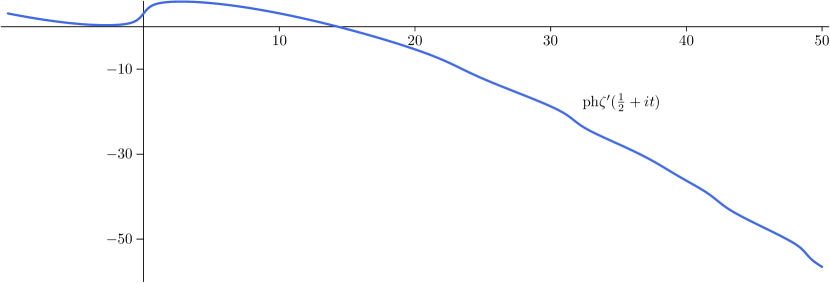
Figure 1. $\operatorname{ph}\zeta^{\prime}({\textstyle\frac{1}{2}}\,+it)$

Proposition 13.

For all $t\in\mathbf{R}$

(17) $$\kappa(t)=\frac{1}{2}-\frac{1}{\pi}\bigl{(}\vartheta(t)+\operatorname{ph}\zeta^{\prime}({\textstyle\frac{1}{2}}\,+it)\bigr{)}.$$

Proof.

By the definition of $\kappa(t)$ and (15) we have

$$\exp\bigl{(}2\pi i\kappa(t)\bigr{)}=-e^{-2i\vartheta(t)}\frac{\zeta^{\prime}({\textstyle\frac{1}{2}}\,-it)}{\zeta^{\prime}({\textstyle\frac{1}{2}}\,+it)}=\exp\bigl{(}\pi i-2i\vartheta(t)-2i\operatorname{ph}\zeta^{\prime}({\textstyle\frac{1}{2}}\,+it)\bigr{)}.$$

Hence there exists an integer $n$ such that

$$2\pi i\kappa(t)=\pi i-2i\vartheta(t)-2i\operatorname{ph}\zeta^{\prime}({\textstyle\frac{1}{2}}\,+it)+2\pi in.$$

For $t=0$ we get $n=0$ and (17) follows. ∎

Corollary 14.

For every real $t$ we have

(18) $$\kappa(t)=-\frac{1}{2}-\frac{1}{\pi}\int_{0}^{t}\Bigl{(}\vartheta^{\prime}(x)+\operatorname{Re}\frac{\zeta^{\prime\prime}({\textstyle\frac{1}{2}}\,+ix)}{\zeta^{\prime}({\textstyle\frac{1}{2}}\,+ix)}\Bigr{)}\,dx.$$

Proof.

In formula (17), we replace $\operatorname{ph}\zeta^{\prime}({\textstyle\frac{1}{2}}\,+it)$ by the integral expression given by (7). ∎

Observing that $-\vartheta(t)$ is the phase of $\zeta(\frac{1}{2}+it)$ we also obtain (see (8))

(19) $$\kappa(t)=-\frac{1}{2}+\frac{1}{\pi}\int_{0}^{t}\operatorname{Re}\Bigl{(}\frac{\zeta^{\prime}(\frac{1}{2}+ix)}{\zeta(\frac{1}{2}+ix)}-\frac{\zeta^{\prime\prime}(\frac{1}{2}+ix)}{\zeta^{\prime}(\frac{1}{2}+ix)}\Bigr{)}\,dx.$$

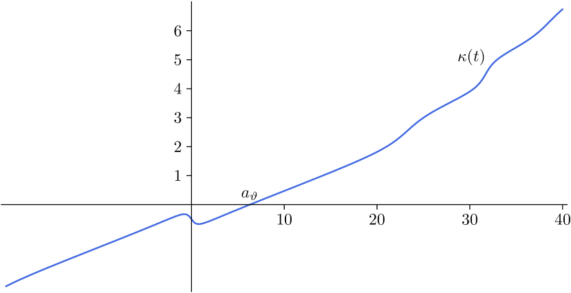
Figure 2. $\kappa(t)$

From (19) we see that $\kappa(t)+\frac{1}{2}$ is an odd function.

Proposition 15.

Choosing the phase of the real analytic function $t\mapsto Z^{\prime}(t)-Z(t)\vartheta^{\prime}(t)$ to be $=\pi/2$ at $t=0$ we will have

(20) $$\kappa(t)=-\frac{1}{\pi}\operatorname{ph}(Z^{\prime}(t)-iZ(t)\,\vartheta^{\prime}(t)).$$

Proof.

Choosing appropriately the phase of $(Z^{\prime}-iZ\vartheta^{\prime})$, it follows from (12) that

$$\vartheta(t)+\operatorname{ph}\zeta^{\prime}({\textstyle\frac{1}{2}}\,+it)=\frac{\pi}{2}+\operatorname{ph}(Z^{\prime}(t)-iZ(t)\vartheta^{\prime}(t)).$$

Thus, by (17)

$$\kappa(t)=-\frac{1}{\pi}\operatorname{ph}(Z^{\prime}(t)-iZ(t)\vartheta^{\prime}(t)).$$

(We have $Z^{\prime}(0)-iZ(0)\vartheta^{\prime}(0)=-i\,3.92264\dots$, so that we have to take the phase of $(Z^{\prime}-iZ\vartheta^{\prime})$ equal to $\pi/2$ at $t=0$.) ∎

Proposition 16.

We have $\kappa(a_{\vartheta})=0$.

Proof.

For $z$ not equal to zero let, as usual, $\operatorname{Arg}z$ be the determination of the argument of $z$ with $-\pi<\operatorname{Arg}z\leq\pi$.

By Proposition 15 for every interval $I$ on which $Z(t)\vartheta^{\prime}(t)\neq 0$ there will exist an integer $n_{I}$ such that

$$\kappa(t)=-\frac{1}{\pi}\operatorname{Arg}(Z^{\prime}(t)-iZ(t)\vartheta^{\prime}(t))+n_{I}.$$

In particular this applies to the interval $I=(0,a_{\vartheta})$. To determine $n_{I}$ in this case observe that $\kappa(0)=-{\textstyle\frac{1}{2}}\,$, $Z^{\prime}(0)=0$, $Z(0)<0$ and $\vartheta^{\prime}(0)<0$, and it follows that $n_{I}=-1$.

Then choose $\varepsilon>0$ small enough. At the point $t=a_{\vartheta}-\varepsilon$ we have $Z^{\prime}(t)<0$, $Z(t)<0$, and $\vartheta^{\prime}(a_{\vartheta})=0$. Since $\kappa(t)$ is continuous and $\vartheta^{\prime}(t)<0$ we get $\operatorname{Arg}(Z^{\prime}(t)-iZ(t)\vartheta^{\prime}(t))$ near $-\pi$ when $t=a_{\vartheta}-\varepsilon$. Taking limits for $\varepsilon\to 0^{+}$ we get $\kappa(a_{\vartheta})=0$, as asserted. ∎

Proposition 17.

For each natural number $n$ we have $\kappa(\xi_{n})=n$.

Proof.

Assuming that $\kappa(\xi_{k})=k$ for $k\leq n$ we will show that $\kappa(\xi_{n+1})=n+1$. The case $n=0$ is slightly different, but similar. We assume now that $n\geq 1$.

In the interval $I_{n}=(\xi_{n},\xi_{n+1})$ we have $Z(t)\vartheta^{\prime}(t)\neq 0$. Therefore

$$\operatorname*{sgn}(Z(t)\vartheta^{\prime}(t))=\operatorname*{sgn}(Z(t))=\nu.$$

By Proposition 15 there is an integer $m$ such that

$$\kappa(t)=m-\frac{1}{\pi}\operatorname{Arg}(Z^{\prime}(t)-iZ(t)\vartheta^{\prime}(t)),\qquad t\in I_{n}.$$

For $y\neq 0$ we have

$$\operatorname{Arg}(x-iy)=\begin{cases}-\arccos\frac{x}{\sqrt{x^{2}+y^{2}}}&y>0\\ \arccos\frac{x}{\sqrt{x^{2}+y^{2}}}&y<0.\end{cases}$$

Therefore,

(21) $$\kappa(t)=m+\frac{\nu}{\pi}\arccos\frac{Z^{\prime}(t)}{\sqrt{Z^{\prime}(t)^{2}+Z(t)^{2}\vartheta^{\prime}(t)^{2}}}\,\qquad t\in I_{n}.$$

Then if $\mu=\operatorname*{sgn}(Z^{\prime}(t))$ we will have

$$\kappa(t)=m+\frac{\nu}{\pi}\arccos\frac{\mu}{\sqrt{1+\frac{Z(t)^{2}}{Z^{\prime}(t)^{2}}\vartheta^{\prime}(t)^{2}}}.$$

For $t>\xi_{n}$ and $t\to\xi_{n}$ we have for some $A>0$, $C>0$ and an integer $\omega\geq 1$

$$Z(t) =\nu A(t-\xi_{n})^{\omega}+\mathop{\hbox{\cmbsy O}}\nolimits(t-\xi_{n})^{\omega+1}$$

$$Z^{\prime}(t) =\nu\omega A(t-\xi_{n})^{\omega-1}+\mathop{\hbox{\cmbsy O}}\nolimits(t-\xi_{n})^{\omega}$$

$$\frac{Z(t)}{Z^{\prime}(t)} =\frac{1}{\omega}(t-\xi_{n})+\mathop{\hbox{\cmbsy O}}\nolimits(t-\xi_{n})^{2}$$

$$\frac{Z(t)^{2}}{Z^{\prime}(t)^{2}}\vartheta^{\prime}(t)^{2} =\frac{C^{2}}{\omega^{2}}(t-\xi_{n})^{2}+\mathop{\hbox{\cmbsy O}}\nolimits(t-\xi_{n})^{3}.$$

Therefore, in a small interval to the right of $\xi_{n}$ the sign of $Z(t)$ is the same as the sign of $Z^{\prime}(t)$, so that $\mu=\nu$. Hence for $\xi_{n}<t<\xi_{n}+\delta$ we have

(22) $$\kappa(t)=m+\frac{\nu}{\pi}\arccos\Bigl{\{}\nu\Bigl{(}1-\frac{1}{2}\frac{C^{2}}{\omega^{2}}(t-\xi_{n})^{2}+\mathop{\hbox{\cmbsy O}}\nolimits(t-\xi_{n})^{3}\Bigr{)}\Bigr{\}}.$$

Observe that for small $x>0$ we have

$$\arccos(1-x)=\sqrt{2}\sqrt{x}+\mathop{\hbox{\cmbsy O}}\nolimits(x^{3/2}),\qquad\arccos(-1+x)=\pi-\sqrt{2}\sqrt{x}+\mathop{\hbox{\cmbsy O}}\nolimits(x^{3/2}).$$

It follows that for $\nu=1$

$$\kappa(t)=m+\frac{1}{\pi}\frac{C}{\omega}(t-\xi_{n})+\mathop{\hbox{\cmbsy O}}\nolimits(t-\xi_{n})^{2}$$

and for $\nu=-1$

$$\kappa(t)=m-1+\frac{1}{\pi}\frac{C}{\omega}(t-\xi_{n})+\mathop{\hbox{\cmbsy O}}\nolimits(t-\xi_{n})^{2}.$$

Taking limits for $t\to\xi_{n}^{+}$ we get

$$n=\kappa(\xi_{n})=\begin{cases}m&\text{when $\nu=1$},\\ m-1&\text{when $\nu=-1$}.\end{cases}$$

Having determined $m$ we move $t$ to the other extreme of the interval $I_{n}$ in (21). Therefore, now $\xi_{n+1}-\delta<t<\xi_{n+1}$ with $\delta$ small enough. We still have $\operatorname*{sgn}Z(t)=\nu$, so that $Z(t)=\nu B(t-\xi_{n+1})^{\varpi}$ with $B>0$. As before we will get $\frac{Z(t)}{Z^{\prime}(t)}=\frac{1}{\varpi}(t-\xi_{n+1})$, but in this case this means that $\operatorname*{sgn}(Z^{\prime}(t))=-\operatorname*{sgn}(Z(t))$ so that $\mu=-\nu$, where now $\mu$ is the sign of $Z^{\prime}(t)$ for $\xi_{n+1}-\delta<t<\xi_{n+1}$. Hence in this case the analogue of (22) is

(23) $$\kappa(t)=m+\frac{\nu}{\pi}\arccos\Bigl{\{}-\nu\Bigl{(}1-\frac{1}{2}\frac{C^{\prime 2}}{\varpi^{2}}(t-\xi_{n+1})^{2}+\mathop{\hbox{\cmbsy O}}\nolimits(t-\xi_{n+1})^{3}\Bigr{)}\Bigr{\}}.$$

It follows that for $\nu=1$

$$\kappa(t)=m+1-\frac{1}{\pi}\frac{C^{\prime}}{\varpi}(\xi_{n+1}-t)+\mathop{\hbox{\cmbsy O}}\nolimits(t-\xi_{n+1})^{2}.$$

Taking limits for $t\to\xi_{n+1}$ we get

$$\kappa(\xi_{n+1})=m+1=n+1=\kappa(\xi_{n})+1$$

and for $\nu=-1$

$$\kappa(t)=m-\frac{1}{\pi}\frac{C^{\prime}}{\varpi}(\xi_{n+1}-t)+\mathop{\hbox{\cmbsy O}}\nolimits(t-\xi_{n+1})^{2}$$

so that in this case

$$\kappa(\xi_{n+1})=m=n+1=\kappa(\xi_{n})+1.$$

∎

Corollary 18.

The function $\kappa(t)$ takes integer values only in the following cases: $\kappa(a_{\vartheta})=0$, $\kappa(-a_{\vartheta})=-1$, $\kappa(\xi_{n})=n$, $\kappa(-\xi_{n})=-n-1$ for all natural numbers $n$.

Proof.

Since $\kappa(t)+{\textstyle\frac{1}{2}}\,$ is an odd function we get $\kappa(-t)=-\kappa(t)-1$, so that $\kappa(-a_{\vartheta})=-1$ and $\kappa(-\xi_{n})=-n-1$.

Assuming that $\kappa(t)\in\mathbf{Z}$, by (16) we must have $\vartheta^{\prime}(t)\zeta(\frac{1}{2}+it)=0$ (recall that if $\zeta^{\prime}(\frac{1}{2}+it)=0$ then $\zeta({\textstyle\frac{1}{2}}\,+it)=0$ so that the quotient $\zeta(\frac{1}{2}+it)/\zeta^{\prime}({\textstyle\frac{1}{2}}\,+it)$ is equal to $0$ in this case). By Corollary 9, for $t>0$, we have $\vartheta^{\prime}(t)=0$ only for $t=a_{\vartheta}$. By definition the positive real numbers $t$ such that $\zeta(\frac{1}{2}+it)=0$ are the numbers $\xi_{n}$. This proves that $\kappa(t)$ is an integer only at the points indicated. ∎

Corollary 19.

For $n=1$, $2$, …the number $\xi_{n}$ is the unique solution of the equation $\kappa(t)=n$.

If we assume the RH and that the zeros are simple, we get that $\gamma_{n}$ is the only solution of the equation $\kappa(t)=n$.

Define $\xi_{0}=a_{\vartheta}$, $\xi_{-1}=-a_{\vartheta}$, $\xi_{-n}=-\xi_{n-1}$, so that for all integers $n\in\mathbf{Z}$ we have $\kappa(\xi_{n})=n$. With these notations we have

Proposition 20.

For any integer $n\in\mathbf{Z}$ and $t$ with $\xi_{n}<t<\xi_{n+1}$ we have $\kappa(\xi_{n})=n<\kappa(t)<n+1=\kappa(\xi_{n+1})$.

Proof.

Since $t\neq\xi_{m}$ the value $\kappa(t)$ is not an integer. If $\kappa(t)<n$, since $\kappa(x)$ is continuous, there will exist $t<t^{\prime}<\xi_{n+1}$ with $\kappa(t^{\prime})=n$, in contradiction with Corollary 18. A similar reasoning rules out the possibility that $\kappa(t)>n+1$. ∎

Proposition 21.

For $t>a_{\vartheta}$, let $N_{00}(t):=\operatorname*{card}\{n\in\mathbf{N}:\xi_{n}\leq t\}$ be the number of real numbers $0<\xi\leq t$ such that $\zeta({\textstyle\frac{1}{2}}\,+i\xi)=0$ counted without multiplicity. Then we have

(24) $$N_{00}(t)=\lfloor\kappa(t)\rfloor.\qquad t>a_{\vartheta}.$$

Proof.

Since $t>a_{\vartheta}=\xi_{0}$ there is an integer $n\geq 0$ such that $\xi_{n}\leq t<\xi_{n+1}$. By definition $N_{00}(t)=n$ and by Proposition 20 $n\leq\kappa(t)<n+1$ so that $\lfloor\kappa(t)\rfloor=n$. ∎

Remark 22.

It is known [BCY] that $N_{0}^{*}(T)$ the number of simple zeros on the line to height $T$ satisfies $\liminf_{T\to\infty}N_{0}^{*}(T)/N(T)\geq 0.4058$, where $N(T)$, as usual, denotes the number of zeros $\beta+i\gamma$ of $\zeta(s)$ with $0<\gamma<T$ counted with their multiplicities. Since $\kappa(t)\geq N_{0}^{*}(t)$ we deduce that $\liminf_{t\to\infty}\kappa(t)/N(t)\geq 0.4058$. In [BH], assuming the RH (but not the simplicity of the zeros) this has been improved to

(25) $$\liminf_{t\to\infty}\kappa(t)/N(t)\geq 0.84665.$$

Proposition 23.

For any real $t$ we have $\kappa(t)=\frac{2k+1}{2}$ with $k\in\mathbf{Z}$ if and only if $Z^{\prime}(t)=0$ and $Z(t)\neq 0$.

Proof.

The function $\vartheta^{\prime}(t)$ only vanishes at $t=\pm a_{\vartheta}$ and at these points the function $Z^{\prime}(t)$ does not vanish ($Z^{\prime}(a_{\vartheta})=-Z^{\prime}(-a_{\vartheta})=-0.18838\cdots$). Hence $Z^{\prime}(t)-iZ(t)\vartheta^{\prime}(t)=0$ only at a point where $Z(t)=Z^{\prime}(t)=0$. Since $Z(t)=0$ there exists $n$ with $t=\xi_{n}$. By Corollary 18 we know that at this point $\kappa(t)\in\mathbf{Z}$.

Let $t$ be a point where $Z(t)\neq 0$ but $Z^{\prime}(t)=0$, then $Z^{\prime}(t)-iZ(t)\vartheta^{\prime}(t)\in i\mathbf{R}^{*}$ and by (20) we have $\kappa(t)=-\frac{1}{\pi}\operatorname{ph}(Z^{\prime}(t)-iZ(t)\vartheta^{\prime}(t))=k+\frac{1}{2}$ for some $k\in\mathbf{Z}$.

If, on the other hand, we assume $\kappa(t)=\frac{2k+1}{2}$, then again by (20), $\operatorname{ph}(Z^{\prime}(t)-iZ(t)\vartheta^{\prime}(t))=-(2k+1)\frac{\pi}{2}$, so that $Z^{\prime}(t)-iZ(t)\vartheta^{\prime}(t)\in i\mathbf{R}$, and certainly we will have $Z^{\prime}(t)=0$ and as we have seen $Z(t)\neq 0$. ∎

5. Hypothesis P  and its consequences.

One may verify that $\kappa^{\prime}(0)$ is negative ($=-0.444016\dots$). In fact $\kappa^{\prime}(t)$ is negative for all $t$ with

$$|t|<a_{\kappa}=0.77985\,35753\,38836\,03051\,82092\,08122\,53710\,71856\,73276\,80740\,38626\,70020\dots$$

We will prove in Proposition 40 that, assuming the RH, $\kappa^{\prime}(t)>0$ for $t>a_{\kappa}$. But we are unable to prove the RH assuming $\kappa^{\prime}(t)>0$ for $t>a_{\kappa}$. However, this appears to be a realistic hypothesis (weaker than the RH):

Hypothesis P.

$\kappa^{\prime}(t)\geq 0$ for $t>a_{\kappa}$.

Some of our propositions will depend on this hypothesis. We will attach the symbol P  to every proposition or theorem whose proof depends on this hypothesis.

Proposition 24 (P).

For each integer $n\in\mathbf{Z}$, with $n\geq 0$, there is a unique real number $\eta_{n+2}$ such that $\xi_{n}<\eta_{n+2}<\xi_{n+1}$, and $Z^{\prime}(\eta_{n+2})=0$. The number $\eta_{n+2}$ is the unique solution to the equation $\kappa(t)=n+\frac{1}{2}$.

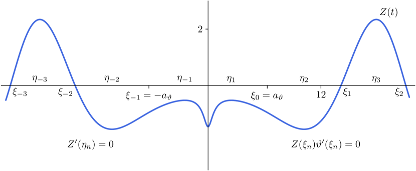
Figure 3. $Z(t)$ near the origin.

Proof.

Since $a_{\kappa}<a_{\vartheta}$ and $\kappa(t)$ is real analytic, the hypothesis P implies that $\kappa(t)$, being analytic is strictly increasing for $t>\xi_{0}:=a_{\vartheta}$. Therefore, for $n\geq 0$ the function $\kappa(t)$ is strictly increasing in the interval $(\xi_{n},\xi_{n+1})$, so that there is only one solution to the equation $\kappa(t)=n+\frac{1}{2}$.

By Proposition 23 the solution $t=\eta_{n+2}$ to the above equation is the only possible solution of the equation $Z^{\prime}(t)=0$ in this interval. ∎

For $n=-1$ we may check numerically that $t=0$ and $t=\pm\,2.4757266\dots$ are solutions to $Z^{\prime}(t)=0$ in the interval $(\xi_{-1},\xi_{0})=(-a_{\vartheta},a_{\vartheta})$.

Using the above it is easy to see that the points where $\kappa(t)=n+\frac{1}{2}$ are the following:

(a) Three points in the interval $(\xi_{-1},\xi_{0})=(a_{-\vartheta},a_{\vartheta})$. These are $\eta_{1}=-\eta_{-1}=2.47572\dots$, and $\eta_{0}=0$ at which $\kappa(\eta_{-1})=\kappa(\eta_{0})=\kappa(\eta_{1})=-\frac{1}{2}$.

(b) A point $\eta_{2}\in(\xi_{0},\xi_{1})$, with $\eta_{2}=10.21207\dots$ at which $\kappa(\eta_{2})=\frac{1}{2}$ and its symmetric $\eta_{-2}=-\eta_{2}$ at which $\kappa(-\eta_{2})=-\frac{3}{2}$.

(c) For each integer $n\geq 1$ a unique point $\eta_{n+2}\in(\xi_{n},\xi_{n+1})$ at which $\kappa(\eta_{n+2})=n+\frac{1}{2}$. Its symmetrical $\eta_{-n-2}\in(\xi_{-n-2},\xi_{-n-1})$ with $\eta_{-n-2}=-\eta_{n+2}$ and $\kappa(\eta_{-n-2})=-\frac{2n+3}{2}$.

One may verify that the minimal value $a_{\gamma}$ of $\kappa(t)$ is

$$a_{\gamma}:=\kappa(a_{\kappa})=-0.67025\,97987\,68599\,50288\,39164\,11968\,66744\,74803\,92790\,09743\,49173\,\dots$$

Since $\kappa$ is strictly increasing on $(a_{\kappa},+\infty)$ with values in $(a_{\gamma},\infty)$ we may define $\gamma(u)$ for $u>a_{\gamma}$ as the inverse function of $\kappa(t)$. $\gamma(u)$ is a real analytic function on $(a_{\gamma},\infty)$ and we will have

$$\gamma(n)=\xi_{n},\qquad\gamma(n+{\textstyle\frac{1}{2}}\,)=\eta_{n+2},\qquad n\geq 0,\quad\text{assuming P}.$$

Of course, assuming the RH with simple zeros we will have $\gamma(n)=\gamma_{n}$.

Proposition 25.

For $t\in\mathbf{R}$ not a multiple zero of $Z(t)$ we have

(26) $$\kappa^{\prime}=\frac{1}{\pi}\frac{ZZ^{\prime}\vartheta^{\prime\prime}+(Z^{\prime})^{2}\vartheta^{\prime}-ZZ^{\prime\prime}\vartheta^{\prime}}{(Z^{\prime})^{2}+(Z\vartheta^{\prime})^{2}},$$

where for short we have written $\kappa^{\prime}$ for $\kappa^{\prime}(t)$, $Z$ for $Z(t)$, etc. Therefore

(27) $$P\quad\Longleftrightarrow\quad ZZ^{\prime}\vartheta^{\prime\prime}+(Z^{\prime})^{2}\vartheta^{\prime}-ZZ^{\prime\prime}\vartheta^{\prime}\geq 0\quad\text{for $t>a_{\kappa}$}.$$

Proof.

For $\xi_{n}<t<\xi_{n+1}$ we have (21) for some constant $m$. Differentiating and simplifying we get (26). Since $\kappa^{\prime}$ is real analytic the equality is true because we are not dividing by $0$. ∎

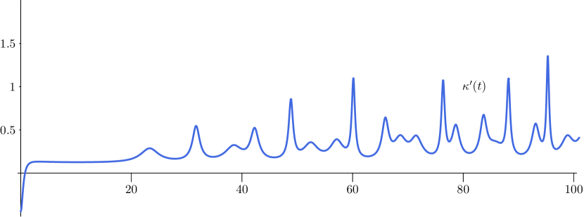
Figure 4. $\kappa^{\prime}(t)$

6. Connection of $\kappa^{\prime}(t)$ with the zeros of $\zeta^{\prime}(s)$.

We will need some known facts (see [S], [LM]*Theorem 9, [B] and [T]*Theorem 11.5(C)) about the zeros of $\zeta^{\prime}(s)$.

Proposition 26.

• For $n\geq 1$ there is a unique real solution $a_{n}$ of $\zeta^{\prime}(s)=0$ with $-2n-2<a_{n}<-2n$, and there are no other zeros of $\zeta^{\prime}(s)$ in $\sigma\leq 0$.

• Let $\rho^{\prime}=\beta^{\prime}+i\gamma^{\prime}$ denote the non real zeros of $\zeta^{\prime}(s)$, and let $N_{1}(T)$ denote the number of non real zeros of $\zeta^{\prime}(s)$ with $0<\gamma<T$. Then

  $$N_{1}(T)=\frac{T}{2\pi}\log\frac{T}{4\pi}-\frac{T}{2\pi}+\mathop{\hbox{\cmbsy O}}\nolimits(\log T).$$

• We have $0<\beta^{\prime}\leq E$ where $E\leq 3$ is a constant. The Riemann Hypothesis is equivalent to $\zeta^{\prime}(s)$ having no zeros in $0<\sigma<1/2$.

We will use $\rho^{\prime}=\beta^{\prime}+i\gamma^{\prime}$ to denote a typical complex zero of $\zeta^{\prime}(s)$. Other times we prefer to denote by $\rho^{\prime}_{n}=\beta^{\prime}_{n}+i\gamma^{\prime}_{n}$ the sequence of zeros with $\gamma^{\prime}_{n}>0$ numbered in such a way that $0<\gamma^{\prime}_{1}\leq\gamma^{\prime}_{2}\leq\cdots$, with the understanding that the ordinate of a zero of multiplicity $m$ appears $m$ times consecutively in this sequence.

Proposition 27.

We have the following Mittag-Leffler expansion

(28) $$\frac{\zeta^{\prime\prime}(s)}{\zeta^{\prime}(s)}=a-\frac{2}{s-1}+\sum_{n=1}^{\infty}\Bigl{(}\frac{1}{s-a_{n}}+\frac{1}{a_{n}}\Bigr{)}+\sum_{\rho^{\prime}}\Bigl{(}\frac{1}{s-\rho^{\prime}}+\frac{1}{\rho^{\prime}}\Bigr{)}$$

where the $a_{n}$ are the real, and $\rho^{\prime}_{n}$ the complex zeros of $\zeta^{\prime}(s)$, and $a=0.18334\dots$ is a constant ($=-2+\zeta^{\prime\prime}(0)/\zeta^{\prime}(0)$).

Proof.

The entire function $f(s)=(s-1)^{2}\zeta^{\prime}(s)$ has the same order as $(s-1)\zeta(s)$ so that $f(s)$ is an entire function of order $1$.

From the above results about the zeros of $\zeta^{\prime}(s)$ it follows easily that the exponent of convergence of the zeros of $f(s)$ is $1$. Also, the series $\sum_{n=1}^{\infty}1/|a_{n}|$ is divergent. Thus we have

(29) $$\zeta^{\prime}(s)=e^{as+b}(s-1)^{-2}\prod_{n=1}^{\infty}\Bigl{(}1-\frac{s}{a_{n}}\Bigr{)}e^{s/a_{n}}\prod_{\rho^{\prime}}\Bigl{(}1-\frac{s}{\rho^{\prime}}\Bigr{)}e^{s/\rho^{\prime}}$$

for some constants $a$ and $b$.

Now we take logarithms and differentiate to get (28). At the point $s=0$ we obtain the equality

$$\frac{\zeta^{\prime\prime}(0)}{\zeta^{\prime}(0)}=a+2$$

from which we get the numerical value for $a$ given in the statement. ∎

Remark 28.

It can be proved that

$$\frac{\zeta^{\prime\prime}(0)}{\zeta^{\prime}(0)}=\frac{\pi^{2}}{12\log 2\pi}-\frac{\gamma^{2}+2\gamma_{1}}{\log 2\pi}+\log 2\pi$$

where $\gamma$ (the Euler constant) and $\gamma_{1}$ are Stieltjes constants appearing as coefficients in the Mittag–Leffler expansion of $\zeta(s)$ at the point $s=1$.

Remark 29.

The constant $b$ in equation (29) is determined by $e^{b}=\zeta^{\prime}(0)=-{\textstyle\frac{1}{2}}\,\log(2\pi)$. So $b$ is complex.

Proposition 30.

We have

(30) $$\pi\kappa^{\prime}(t)=A+f(t)+\sum_{\rho^{\prime}=\beta^{\prime}+i\gamma^{\prime}}\frac{\beta^{\prime}-1/2}{(1/2-\beta^{\prime})^{2}+(t-\gamma^{\prime})^{2}}$$

where $A$ is a constant and $f(t)$ is a bounded continuous function such that $f(t)=\mathop{\hbox{\cmbsy O}}\nolimits(t^{-1})$ as $t\to+\infty$.

Remark 31.

The exact definition of $f(t)$ is given in (33).

Remark 32.

In Corollary 39 we will prove that $A=\frac{1}{2}\log 2$.

Proof.

From (18) we get

(31) $$\pi\kappa^{\prime}(t)=-\vartheta^{\prime}(t)-\operatorname{Re}\frac{\zeta^{\prime\prime}({\textstyle\frac{1}{2}}\,+it)}{\zeta^{\prime}({\textstyle\frac{1}{2}}\,+it)}.$$

Now in (28) we put $s=1/2+it$ and take real parts

$$\operatorname{Re}\frac{\zeta^{\prime\prime}(1/2+it)}{\zeta^{\prime}(1/2+it)}=a+\frac{4}{1+4t^{2}}+\sum_{n=1}^{\infty}\Bigl{(}\frac{1/2-a_{n}}{(1/2-a_{n})^{2}+t^{2}}+\frac{1}{a_{n}}\Bigr{)}\\ +\sum_{\rho^{\prime}=\beta^{\prime}+i\gamma^{\prime}}\Bigl{(}\frac{1/2-\beta^{\prime}}{(1/2-\beta^{\prime})^{2}+(t-\gamma^{\prime})^{2}}+\frac{\beta^{\prime}}{\beta^{\prime}{}^{2}+\gamma^{\prime}{}^{2}}\Bigr{)}.$$

Hence from (31) and (10) we get

$$\pi\kappa^{\prime}(t)=A-\frac{2}{1+4t^{2}}+\sum_{n=1}^{\infty}\Bigl{(}\frac{2(4n+1)}{(4n+1)^{2}+4t^{2}}-\frac{1/2-a_{n}}{(1/2-a_{n})^{2}+t^{2}}\Bigr{)}\\ +\sum_{\rho^{\prime}=\beta^{\prime}+i\gamma^{\prime}}\frac{\beta^{\prime}-1/2}{(1/2-\beta^{\prime})^{2}+(t-\gamma^{\prime})^{2}}$$

where

(32) $$A=\frac{1}{2}(\gamma+\log\pi)-a-\sum_{n=1}^{\infty}\frac{2\beta^{\prime}_{n}}{\beta^{\prime}_{n}{}^{2}+\gamma^{\prime}_{n}{}^{2}}-\sum_{n=1}^{\infty}\Bigl{(}\frac{1}{2n}+\frac{1}{a_{n}}\Bigr{)}.$$

We put

(33) $$f(t)=-\frac{2}{1+4t^{2}}+\sum_{n=1}^{\infty}\Bigl{(}\frac{2(4n+1)}{(4n+1)^{2}+4t^{2}}-\frac{1/2-a_{n}}{(1/2-a_{n})^{2}+t^{2}}\Bigr{)}.$$

Now observe that the terms of the sum can be written as

$$\frac{(2n+1/2)}{(2n+1/2)^{2}+t^{2}}-\frac{1/2-a_{n}}{(1/2-a_{n})^{2}+t^{2}}=\int_{2n+1/2}^{1/2-a_{n}}\frac{x^{2}-t^{2}}{(x^{2}+t^{2})^{2}}\,dx.$$

The intervals $(2n+1/2,1/2-a_{n})$ do not intersect, so that for $|t|<T$ the absolute values of the terms of the sum are bounded by

$$\sum_{n=1}^{\infty}\Bigl{|}\frac{2(4n+1)}{(4n+1)^{2}+4t^{2}}-\frac{1/2-a_{n}}{(1/2-a_{n})^{2}+t^{2}}\Bigr{|}\leq\int_{5/2}^{+\infty}\frac{|x^{2}-t^{2}|}{(x^{2}+t^{2})^{2}}\,dx\\ \leq\int_{5/2}^{+\infty}\frac{T^{2}+x^{2}}{x^{4}}\,dx<+\infty.$$

This proves that $f(t)$ is a continuous function.

Also for $t>1$ we will have

(34) $$|f(t)|\leq\frac{2}{1+4t^{2}}+\int_{0}^{+\infty}\frac{|x^{2}-t^{2}|}{(x^{2}+t^{2})^{2}}\,dx=\frac{2}{1+4t^{2}}+\frac{1}{t}.$$

∎

Remark 33.

It can be shown that the zero $a_{n-1}$ contained in $(-2n,-2n+2)$ satisfies $2n+a_{n-1}\sim 1/\log(n/\pi)$. This information can be used to show that $f(t)=\mathop{\hbox{\cmbsy O}}\nolimits(1/t\log t)$. In this way we may improve the error term in (36) from $\mathop{\hbox{\cmbsy O}}\nolimits(\log t)$ to $\mathop{\hbox{\cmbsy O}}\nolimits(\log\log t)$.

We introduce some notation: if $t>0$ and $n\geq 1$ let $\operatorname{\varphi}(t,\rho^{\prime}_{n})=\operatorname{\varphi}_{n}(t)$ be the angle at $\rho^{\prime}_{n}$ of the triangle with vertices at $\rho^{\prime}_{n}=\beta^{\prime}_{n}+i\gamma^{\prime}_{n}$, $1/2-it$ and $1/2+it$. We consider this angle expressed in radians positive if $\beta^{\prime}_{n}>1/2$ and negative if $\beta^{\prime}_{n}<1/2$, and we put $\operatorname{\varphi}_{n}(t)=0$ when $\beta^{\prime}_{n}={\textstyle\frac{1}{2}}\,$. In other words with $s={\textstyle\frac{1}{2}}\,+it$ and $\rho^{\prime}=\beta^{\prime}+i\gamma^{\prime}$ we have

(35) $$\operatorname{\varphi}(t,\beta^{\prime}+i\gamma^{\prime})=\arctan\frac{t-\gamma^{\prime}}{\beta^{\prime}-\frac{1}{2}}+\arctan\frac{t+\gamma^{\prime}}{\beta^{\prime}-\frac{1}{2}}=\operatorname{Arg}\frac{\overline{s}-\rho^{\prime}}{s-\rho^{\prime}}\qquad(\beta^{\prime}\neq{\textstyle\frac{1}{2}}\,).$$

Proposition 34.

For $t>0$ we have

(36) $$\pi\kappa(t)=At+\sum_{n=1}^{\infty}\operatorname{\varphi}_{n}(t)+\mathop{\hbox{\cmbsy O}}\nolimits(\log t)$$

where the sum is extended over all zeros $\rho^{\prime}_{n}=\beta^{\prime}_{n}+i\gamma^{\prime}_{n}$ of $\zeta^{\prime}(s)$ with $\gamma^{\prime}_{n}>0$.

Proof.

By (18) and (30) we have

$$\pi\kappa(t)=-\frac{\pi}{2}+At+\int_{0}^{t}f(x)\,dx+\int_{0}^{t}\sum_{\rho^{\prime}=\beta^{\prime}+i\gamma^{\prime}}\frac{\beta^{\prime}-{\textstyle\frac{1}{2}}\,}{({\textstyle\frac{1}{2}}\,-\beta^{\prime})^{2}+(x-\gamma^{\prime})^{2}}\,dx.$$

Observe that if $\beta^{\prime}={\textstyle\frac{1}{2}}\,$ then the corresponding term does not contribute to the sum.

Thus

$$\pi\kappa(t)=-\frac{\pi}{2}+At+\int_{0}^{t}f(x)\,dx+\sum_{\rho^{\prime}=\beta^{\prime}+i\gamma^{\prime}}\Bigl{\{}\arctan\frac{t-\gamma^{\prime}}{\beta^{\prime}-{\textstyle\frac{1}{2}}\,}+\arctan\frac{\gamma^{\prime}}{\beta^{\prime}-{\textstyle\frac{1}{2}}\,}\Bigr{\}}$$

where the terms with $\beta^{\prime}_{n}={\textstyle\frac{1}{2}}\,$ should be omitted. It is easy to see that the sum of the terms corresponding to $\rho^{\prime}_{n}=\beta^{\prime}_{n}+i\gamma^{\prime}_{n}$ and $\overline{\rho^{\prime}_{n}}=\beta^{\prime}_{n}-i\gamma^{\prime}_{n}$ add up to exactly $\operatorname{\varphi}_{n}(t)$. (This is the reason we made the convention about the sign of $\operatorname{\varphi}_{n}(t)$). Thus we arrive at

$$\pi\kappa(t)=-\frac{\pi}{2}+At+\int_{0}^{t}f(x)\,dx+\sum_{n=1}^{\infty}\operatorname{\varphi}_{n}(t).$$

Now, since $f(t)=\mathop{\hbox{\cmbsy O}}\nolimits(t^{-1})$ we can write this as

$$\pi\kappa(t)=At+\sum_{n=1}^{\infty}\operatorname{\varphi}_{n}(t)+\mathop{\hbox{\cmbsy O}}\nolimits(\log t).$$

∎

7. Counting the zeros of $\zeta(s)$.

The exact value of the constant $A$ in (36) can be obtained in two ways. One by computing the constants in the Mittag-Leffler expansion of related functions and the second, more interesting for us, by comparing two different counts of the number of zeros of $\zeta(s)$. We will present this second proof. We need some definitions:

Let

$$N_{-}(T) =\#\{\rho=\beta+i\gamma\phantom{0}|\phantom{0}\zeta(\rho)=0,\phantom{0}\beta<{\textstyle\frac{1}{2}}\,,\phantom{0}0<\gamma\leq T\}$$

$$N_{0}(T) =\#\{\rho={\textstyle\frac{1}{2}}\,+i\gamma\phantom{0}|\phantom{0}\zeta(\rho)=0,\phantom{0}0<\gamma\leq T\}$$

$$N^{\prime}(T) =\#\{\rho^{\prime}=\beta^{\prime}+i\gamma^{\prime}\phantom{0}|\phantom{0}\zeta^{\prime}(\rho^{\prime})=0,\phantom{0}0<\gamma^{\prime}\leq T\}$$

$$N^{\prime}_{-}(T) =\#\{\rho^{\prime}=\beta^{\prime}+i\gamma^{\prime}\phantom{0}|\phantom{0}\zeta^{\prime}(\rho^{\prime})=0,\phantom{0}\beta^{\prime}<{\textstyle\frac{1}{2}}\,,\phantom{0}0<\gamma^{\prime}\leq T\}$$

$$N^{\prime}_{0}(T) =\#\{\rho^{\prime}={\textstyle\frac{1}{2}}\,+i\gamma^{\prime}\phantom{0}|\phantom{0}\zeta^{\prime}(\rho^{\prime})=0,\phantom{0}0<\gamma^{\prime}\leq T\}$$

$$N^{\prime}_{+}(T) =\#\{\rho^{\prime}=\beta^{\prime}+i\gamma^{\prime}\phantom{0}|\phantom{0}\zeta^{\prime}(\rho^{\prime})=0,\phantom{0}\beta^{\prime}>{\textstyle\frac{1}{2}}\,,\phantom{0}0<\gamma^{\prime}\leq T\}.$$

In all these cases, as usual, we count the zeros with their multiplicities. But we also need to consider another count $N_{00}(T)$ which is the number of real numbers $0<\xi\leq T$ such that $\zeta({\textstyle\frac{1}{2}}\,+i\xi)=0$, but in these cases we do not count multiplicities.

Taking account of Proposition 10 it is clear that

(37) $$N_{0}(T)-N_{00}(T)=N^{\prime}_{0}(T)$$

which equals the number of zeros of $\zeta^{\prime}(s)$ on the critical line with $0<\gamma^{\prime}\leq T$.

We know some relations between these counts:

(i) Backlund refining previous work of von Mangoldt (see Edwards, [E]*Section 6.7) gave a complete proof of Riemann’s assertion

(38) $$N(T)=N_{0}(T)+2N_{-}(T)=\frac{T}{2\pi}\log\frac{T}{2\pi}-\frac{T}{2\pi}+\mathop{\hbox{\cmbsy O}}\nolimits(\log T).$$

(ii) Berndt [B] proved the corresponding result for $\zeta^{\prime}(s)$

(39) $$N^{\prime}(T)=N^{\prime}_{-}(T)+N^{\prime}_{0}(T)+N^{\prime}_{+}(T)=\frac{T}{2\pi}\log\frac{T}{4\pi}-\frac{T}{2\pi}+\mathop{\hbox{\cmbsy O}}\nolimits(\log T).$$

(iii) Levinson and Montgomery [LM] showed that

(40) $$N_{-}(T)=N^{\prime}_{-}(T)+\mathop{\hbox{\cmbsy O}}\nolimits(\log T).$$

(iv) From our Proposition 21 we get that

(41) $$\kappa(t)=N_{00}(t)+\mathop{\hbox{\cmbsy O}}\nolimits(1).$$

Finally, in Proposition 37 we will prove a new relation (42). First we prove two lemmas about the zeros of $\zeta^{\prime}(s)$.

Table 1. First non-trivial zeros of $\zeta(s)$ and $\zeta^{\prime}(s)$

$\beta_{n}+i\gamma_{n}$	$\beta^{\prime}_{n}+i\gamma^{\prime}_{n}$
$0.5+i\,14.13472\,51417$	$2.46316\,18694+i\,23.29832\,04927$
$0.5+i\,21.02203\,96387$	$1.28649\,68222+i\,31.70825\,00831$
$0.5+i\,25.01085\,75801$	$2.30757\,00637+i\,38.48998\,31730$
$0.5+i\,30.42487\,61258$	$1.38276\,36057+i\,42.29096\,45545$
$0.5+i\,32.93506\,15877$	$0.96468\,56227+i\,48.84715\,99050$
$0.5+i\,37.58617\,81588$	$2.10169\,99009+i\,52.43216\,12451$
$0.5+i\,40.91871\,90121$	$1.89595\,97624+i\,57.13475\,31990$

Lemma 35.

For $t>0$ we have

$$\sum_{0<\gamma^{\prime}_{n}<t-1}\frac{1}{t-\gamma^{\prime}_{n}}=\mathop{\hbox{\cmbsy O}}\nolimits(\log^{2}t).$$

Proof.

Put

$$N^{\prime}(t)=\frac{t}{2\pi}\log\frac{t}{4\pi}-\frac{t}{2\pi}+R(t)$$

where $R(t)=\mathop{\hbox{\cmbsy O}}\nolimits(\log t)$ by Berndt’s Theorem. The first zero of $\zeta^{\prime}(s)$ is $\rho^{\prime}\approx 2.46316+23.29832i$ so that $N^{\prime}(4\pi)=0$ and consequently $R(4\pi)=2$. We have

$$\sum_{0<\gamma^{\prime}_{n}<t-1}\frac{1}{t-\gamma^{\prime}_{n}}=\int_{4\pi}^{t-1}\frac{dN^{\prime}(x)}{t-x}=\frac{1}{2\pi}\int_{4\pi}^{t-1}\frac{\log(x/4\pi)}{t-x}\,dx+\int_{4\pi}^{t-1}\frac{dR(x)}{t-x}$$

$$\leq\log(t/4\pi)\frac{\log(t-4\pi)}{2\pi}+R(t-1)+\int_{4\pi}^{t-1}\frac{|R(x)|}{(t-x)^{2}}\,dx.$$

Since $R(x)=\mathop{\hbox{\cmbsy O}}\nolimits(\log x)$ all the above terms are $\mathop{\hbox{\cmbsy O}}\nolimits(\log^{2}t)$. ∎

Lemma 36.

For $t\to+\infty$ we have

$$\sum_{\gamma^{\prime}_{n}>t+1}\frac{1}{\gamma^{\prime}_{n}{}^{2}-t^{2}}=\mathop{\hbox{\cmbsy O}}\nolimits\Bigl{(}\frac{\log^{2}t}{t}\Bigr{)}.$$

Proof.

Retaining the notations of the previous lemma we have

$$\sum_{\gamma^{\prime}_{n}>t+1}\frac{1}{\gamma^{\prime}_{n}{}^{2}-t^{2}}=\int_{t+1}^{+\infty}\frac{dN^{\prime}(x)}{x^{2}-t^{2}}=\frac{1}{2\pi}\int_{t+1}^{\infty}\frac{\log(x/4\pi)}{x^{2}-t^{2}}\,dx+\int_{t+1}^{+\infty}\frac{dR(x)}{x^{2}-t^{2}}.$$

For $t>4\pi$ the first integral is less than or equal to $C\log^{2}t/t$:

$$\frac{1}{2\pi}\int_{t+1}^{\infty}\frac{\log(x/4\pi)}{x^{2}-t^{2}}\,dx\leq\frac{2\log t}{2\pi}\int_{t+1}^{t^{2}}\frac{dx}{x^{2}-t^{2}}+\int_{t^{2}}^{+\infty}\frac{\sqrt{x}}{x^{2}-t^{2}}\,dx$$

$$=\frac{\log t}{2\pi t}\Bigl{(}\log\frac{t-1}{t+1}+\log(2t+1)\Bigr{)}+t^{-1/2}\int_{t}^{+\infty}\frac{\sqrt{y}}{y^{2}-1}\,dy\leq\frac{(\log t)^{2}}{\pi t}+\frac{4}{t}.$$

Now we bound the second integral

$$\int_{t+1}^{+\infty}\frac{dR(x)}{x^{2}-t^{2}}=-\frac{R(t+1)}{2t+1}+\int_{t+1}^{+\infty}\frac{R(x)}{(x^{2}-t^{2})^{2}}2x\,dx.$$

For $x>t+1$ we have $x/(x^{2}-t^{2})<1$, and $|R(x)|\leq C\log x$. Thus we have

$$\int_{t+1}^{+\infty}\frac{dR(x)}{x^{2}-t^{2}}\leq c_{1}\frac{\log t}{t}+c_{2}\int_{t+1}^{+\infty}\frac{\log x}{x^{2}-t^{2}}\,dx.$$

Finally, this integral is bounded exactly as the first integral. ∎

Proposition 37.

For $t\to+\infty$

(42) $$\pi\kappa(t)=At+\pi N^{\prime}_{+}(t)-\pi N^{\prime}_{-}(t)+\mathop{\hbox{\cmbsy O}}\nolimits(\log^{2}t).$$

Proof.

By (36) we have to show that

$$\sum_{\gamma^{\prime}_{n}>0}\operatorname{\varphi}_{n}(t)=\pi N^{\prime}_{+}(t)-\pi N^{\prime}_{-}(t)+\mathop{\hbox{\cmbsy O}}\nolimits(\log^{2}t).$$

To this end we will show that

$$\sum_{\begin{subarray}{c}\gamma^{\prime}_{n}>0\\ \beta^{\prime}_{n}>{\textstyle\frac{1}{2}}\,\end{subarray}}\operatorname{\varphi}_{n}(t)=\pi N^{\prime}_{+}(t)+\mathop{\hbox{\cmbsy O}}\nolimits(\log^{2}t);\qquad\sum_{\begin{subarray}{c}\gamma^{\prime}_{n}>0\\ \beta^{\prime}_{n}<{\textstyle\frac{1}{2}}\,\end{subarray}}\operatorname{\varphi}_{n}(t)=-\pi N^{\prime}_{-}(t)+\mathop{\hbox{\cmbsy O}}\nolimits(\log^{2}t).$$

To simplify the notation we will write $\sideset{}{{}^{+}}{\sum}$ to denote a sum restricted to $\beta^{\prime}_{n}>{\textstyle\frac{1}{2}}\,$ and $\sideset{}{{}^{-}}{\sum}$ for a sum restricted to $\beta^{\prime}_{n}<{\textstyle\frac{1}{2}}\,$.

We split the sums into three terms

$$\sideset{}{{}^{+}}{\sum}_{\gamma^{\prime}_{n}>0}\operatorname{\varphi}_{n}(t)=\sideset{}{{}^{+}}{\sum}_{0<\gamma^{\prime}_{n}<t-1}\operatorname{\varphi}_{n}(t)+\sideset{}{{}^{+}}{\sum}_{|\gamma^{\prime}_{n}-t|\leq 1}\operatorname{\varphi}_{n}(t)+\sideset{}{{}^{+}}{\sum}_{\gamma^{\prime}_{n}>t+1}\operatorname{\varphi}_{n}(t).$$

The middle sum is $\mathop{\hbox{\cmbsy O}}\nolimits(\log t)$ because each term is (in absolute value) less than $\pi$ and the number of terms is $\mathop{\hbox{\cmbsy O}}\nolimits(\log t)$. In the first sum the summands are approximately $\pi$ (or $-\pi$). Thus we arrive at

$$\sideset{}{{}^{+}}{\sum}_{\gamma^{\prime}_{n}>0}\operatorname{\varphi}_{n}(t)=\pi N^{\prime}_{+}(t)+\sideset{}{{}^{+}}{\sum}_{0<\gamma^{\prime}_{n}<t-1}\bigl{\{}\operatorname{\varphi}_{n}(t)-\pi\bigr{\}}+\sideset{}{{}^{+}}{\sum}_{\gamma^{\prime}_{n}>t+1}\operatorname{\varphi}_{n}(t)+\mathop{\hbox{\cmbsy O}}\nolimits(\log t)$$

and

$$\sideset{}{{}^{-}}{\sum}_{\gamma^{\prime}_{n}>0}\operatorname{\varphi}_{n}(t)=-\pi N^{\prime}_{-}(t)+\sideset{}{{}^{-}}{\sum}_{0<\gamma^{\prime}_{n}<t-1}\bigl{\{}\operatorname{\varphi}_{n}(t)+\pi\bigr{\}}+\sideset{}{{}^{-}}{\sum}_{\gamma^{\prime}_{n}>t+1}\operatorname{\varphi}_{n}(t)+\mathop{\hbox{\cmbsy O}}\nolimits(\log t).$$

It follows that

$$\sum_{\gamma^{\prime}_{n}>0}\operatorname{\varphi}_{n}(t)=\pi N^{\prime}_{+}(t)-\pi N^{\prime}_{-}(t)+\sum_{0<\gamma^{\prime}_{n}<t-1}\bigl{\{}\operatorname{\varphi}_{n}(t)\pm\pi\bigr{\}}+\sum_{\gamma^{\prime}_{n}>t+1}\operatorname{\varphi}_{n}(t)+\mathop{\hbox{\cmbsy O}}\nolimits(\log t)$$

where we must use the $+$ sign when $\beta^{\prime}_{n}<{\textstyle\frac{1}{2}}\,$ and the $-$ sign when $\beta^{\prime}_{n}>{\textstyle\frac{1}{2}}\,$.

Now for $0<\gamma^{\prime}_{n}<t-1$ and $\beta^{\prime}_{n}>{\textstyle\frac{1}{2}}\,$ we have

$$0<\pi-\operatorname{\varphi}_{n}(t)<\arctan\frac{\beta^{\prime}_{n}-{\textstyle\frac{1}{2}}\,}{t-\gamma^{\prime}_{n}}+\arctan\frac{\beta^{\prime}_{n}-{\textstyle\frac{1}{2}}\,}{t+\gamma^{\prime}_{n}}<2\arctan\frac{\beta^{\prime}_{n}-{\textstyle\frac{1}{2}}\,}{t-\gamma^{\prime}_{n}}<\frac{6}{t-\gamma^{\prime}_{n}}$$

and in the case $\beta^{\prime}_{n}<{\textstyle\frac{1}{2}}\,$ analogously

$$0<\pi+\operatorname{\varphi}_{n}(t)<\arctan\frac{{\textstyle\frac{1}{2}}\,-\beta^{\prime}_{n}}{t-\gamma^{\prime}_{n}}+\arctan\frac{{\textstyle\frac{1}{2}}\,-\beta^{\prime}_{n}}{t+\gamma^{\prime}_{n}}<2\arctan\frac{{\textstyle\frac{1}{2}}\,-\beta^{\prime}_{n}}{t-\gamma^{\prime}_{n}}<\frac{1}{t-\gamma^{\prime}_{n}}.$$

Also, for $\gamma^{\prime}_{n}>t+1$ and $\beta^{\prime}_{n}>{\textstyle\frac{1}{2}}\,$

$$0<\operatorname{\varphi}_{n}(t)=\arctan\frac{2(\beta^{\prime}_{n}-{\textstyle\frac{1}{2}}\,)t}{(\beta^{\prime}_{n}-{\textstyle\frac{1}{2}}\,)^{2}+\gamma^{\prime}_{n}{}^{2}-t^{2}}<\frac{6t}{\gamma^{\prime}_{n}{}^{2}-t^{2}}$$

and for $\beta^{\prime}_{n}<{\textstyle\frac{1}{2}}\,$ the absolute value $|\operatorname{\varphi}_{n}(t)|$ is bounded by the same quantity.

Thus applying the two above lemmas we find that

$$\sum_{\gamma^{\prime}_{n}>0}\operatorname{\varphi}_{n}(t)=\pi N^{\prime}_{+}(t)-\pi N^{\prime}_{-}(t)+\mathop{\hbox{\cmbsy O}}\nolimits(\log^{2}t).$$

∎

Corollary 38.

For $t\to+\infty$

(43) $$N_{00}(t)=\frac{A}{\pi}t+N^{\prime}_{+}(t)-N^{\prime}_{-}(t)+\mathop{\hbox{\cmbsy O}}\nolimits(\log^{2}t).$$

Proof.

Combine (42) with (41). ∎

Corollary 39.

The constant $A$ is equal to $\frac{1}{2}\log 2$.

Proof.

Write $f(t)\circeq g(t)$ to denote that $f(t)-g(t)=\mathop{\hbox{\cmbsy O}}\nolimits(\log^{2}t)$. (In the same way as congruences we can operate with $\circeq$ as if it were an equality sign between equivalence classes). With this notation we have

$$N(t) \circeq\frac{t}{2\pi}\log\frac{t}{2\pi}-\frac{t}{2\pi}$$ by (38)

$$\circeq N_{0}(t)+2N_{-}(t)$$ trivially

$$\circeq N_{0}(t)+2N^{\prime}_{-}(t)$$ by (40)

$$\circeq N_{0}(t)-N_{00}(t)+\frac{A}{\pi}t+N^{\prime}_{+}(t)+N^{\prime}_{-}(t)$$ by (43)

$$\circeq N_{0}(t)-N_{00}(t)+\frac{A}{\pi}t-N^{\prime}_{0}(t)+\frac{t}{2\pi}\log\frac{t}{4\pi}-\frac{t}{2\pi}$$ by (39)

$$\circeq\frac{A}{\pi}t+\frac{t}{2\pi}\log\frac{t}{4\pi}-\frac{t}{2\pi}$$ by (37)

We thus have

$$\frac{t}{2\pi}\log\frac{t}{2\pi}-\frac{t}{2\pi}\circeq\frac{A}{\pi}t+\frac{t}{2\pi}\log\frac{t}{4\pi}-\frac{t}{2\pi}$$

from which we deduce

$$\frac{A}{\pi}t\circeq\frac{t}{2\pi}\log 2.$$

Hence $A={\textstyle\frac{1}{2}}\,\log 2$. ∎

Proposition 40.

The Riemann hypothesis implies the Hypothesis $P$.

Proof.

The Riemann hypothesis is equivalent to $\beta^{\prime}>{\textstyle\frac{1}{2}}\,$ for every zero $\rho^{\prime}=\beta^{\prime}+i\gamma^{\prime}$, and it follows by (30) that if the Riemann hypothesis is true, then $\pi\kappa^{\prime}(t)>A+f(t)$. Since $A=\frac{1}{2}\log 2$, applying (34) we easily see that $\kappa^{\prime}(t)>0$ for $t>3.4$ if we assume the RH. It is clear that there is an $a_{\kappa}\geq 0$ such that $\kappa^{\prime}(t)>0$ for $t>a_{\kappa}$ and $a_{\kappa}<3.4$. ∎

8. Connections between the zeros of $\zeta(s)$ and $\zeta^{\prime}(s)$.

Proposition 41.

Let $\frac{1}{2}+i\xi$ be a zero of $\zeta(s)$ of multiplicity $\omega$ on the critical line, then

(44) $$\kappa^{\prime}(\xi)=\frac{1}{\pi\omega}\vartheta^{\prime}(\xi).$$

Proof.

Since $\zeta(\frac{1}{2}+it)=e^{-i\vartheta(t)}Z(t)$ the function $Z(t)$ has a zero of multiplicity $\omega$ at $t=\xi$. Hence $\lim_{t\to\xi}\frac{Z(t)}{Z^{\prime}(t)}=0$, and for $\omega\geq 2$, $\lim_{t\to\xi}\frac{Z(t)}{Z^{\prime}(t)}\frac{Z^{\prime\prime}(t)}{Z^{\prime}(t)}=\frac{\omega-1}{\omega}$. When $\omega=1$ this second limit is equal to $0=\frac{\omega-1}{\omega}$.

Hence for $0<|t-\xi|<\delta$ we have $Z(t)$, $Z^{\prime}(t)$ and $Z^{\prime\prime}(t)\neq 0$ and by (26) we have

$$\lim_{t\to\xi}\kappa^{\prime}(t)=\lim_{t\to\xi}\frac{1}{\pi}\frac{\frac{Z}{Z^{\prime}}\vartheta^{\prime\prime}+\vartheta^{\prime}-\frac{Z}{Z^{\prime}}\frac{Z^{\prime\prime}}{Z^{\prime}}\vartheta^{\prime}}{1+\left(\frac{Z}{Z^{\prime}}\vartheta^{\prime}\right)^{2}}=\frac{1}{\pi}\Bigl{(}\vartheta^{\prime}(\xi)-\frac{\omega-1}{\omega}\vartheta^{\prime}(\xi)\Bigr{)}=\frac{1}{\pi\omega}\vartheta^{\prime}(\xi).$$

∎

Assuming the RH and the simplicity of zeros we have

$$\int_{a_{\vartheta}}^{\gamma_{n}}\kappa^{\prime}(t)\,dt=n.$$

Hence the mean value of $\kappa^{\prime}(t)$ in $[0,t]$ is $\frac{N(t)}{t}$ which is approximately equal to $\vartheta^{\prime}(t)/\pi$. The above Proposition says that, assuming only the simplicity of zeros, at the points $\xi_{n}$ the value $\kappa^{\prime}(\xi_{n})$ is just equal to this density.

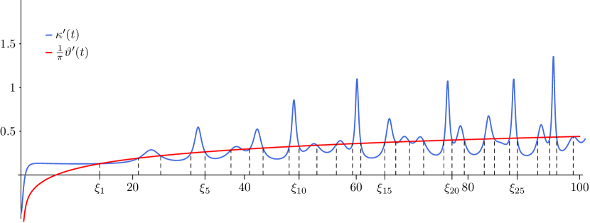
Figure 5. $\kappa(t)$

Figure 5 illustrates two ways in which the zeros of $\zeta^{\prime}(s)$ determine the $\xi_{n}$ (assuming only simplicity of the zeros of zeta). First $\xi_{n}$ is determined from $\kappa^{\prime}(t)$ by the equation

(45) $$\int_{\xi_{0}}^{\xi_{n}}\kappa^{\prime}(t)\,dt=n\quad\text{or}\quad\int_{\xi_{n-1}}^{\xi_{n}}\kappa^{\prime}(t)\,dt=1.$$

Second, the points $\xi_{n}$ are intersections of the two curves $\kappa^{\prime}(t)$ and $\vartheta^{\prime}(t)/\pi$. Although, as we see in figure 5 not all these intersections correspond to points $\xi_{n}$.

We can see how two close $\xi_{n}$ correspond to a peak in the graph of $\kappa^{\prime}(t)$ that, according to equation (30) will be produced by one or more zeros $\beta^{\prime}+i\gamma^{\prime}$ of $\zeta^{\prime}(s)$ with a relatively small $\beta^{\prime}-\frac{1}{2}$. Observe that equation (30) shows that $\kappa^{\prime}(t)$ is fully determined by the zeros of $\zeta^{\prime}(s)$.

Following these ideas we may improve (but assuming the RH) a theorem due to M. Z. Garaev, C. Y. Yıldırım [GY]. For any given zero $\rho^{\prime}=\beta^{\prime}+i\gamma^{\prime}$ of $\zeta^{\prime}(s)$ let $\gamma_{c}$ be of all ordinates of zeros of $\zeta(s)$, the one for which $|\gamma_{c}-\gamma^{\prime}|$ is smallest (if there are more than one such zero of $\zeta(s)$, take $\gamma_{c}$ to be the imaginary part of any one of them). Garaev and Yıldırım prove unconditionally that $|\gamma_{c}-\gamma^{\prime}|\ll|\beta^{\prime}-{\textstyle\frac{1}{2}}\,|^{\frac{1}{2}}$.

Proposition 42 (RH).

Assuming the RH, we have for any zero $\beta^{\prime}+i\gamma^{\prime}$ of $\zeta^{\prime}(s)$

$$|\gamma_{c}-\gamma^{\prime}|\leq 1.9\;|\beta^{\prime}-{\textstyle\frac{1}{2}}\,|^{\frac{1}{2}}.$$

Proof.

Assuming the RH, $\beta^{\prime}>1/2$ so that by equation (30) we will have

$$\kappa^{\prime}(t)\geq\frac{1}{2\pi}\log 2+\frac{f(t)}{\pi}+\frac{1}{\pi}\frac{\beta^{\prime}-\frac{1}{2}}{(\beta^{\prime}-\frac{1}{2})^{2}+(t-\gamma^{\prime})^{2}}.$$

We will find an $a>0$ so that

$$\kappa(\gamma^{\prime}+a)-\kappa(\gamma^{\prime}-a)\geq\frac{a\log 2}{\pi}+\frac{2}{\pi}\arctan\frac{a}{\beta^{\prime}-1/2}+\frac{1}{\pi}\int_{\gamma^{\prime}-a}^{\gamma^{\prime}+a}f(t)\,dt>1.$$

Then there will be a point $\xi\in[\gamma^{\prime}-a,\gamma^{\prime}+a]$ such that $\kappa(\xi)\in\mathbf{Z}$. Then by Corollary 18 $\zeta(\frac{1}{2}+i\xi)=0$, so that the ordinate $\gamma_{c}$ of the nearest zero of $\zeta(s)$ will satisfy $|\gamma_{c}-\gamma^{\prime}|\leq a$.

By (34), for $t>20$ we have $|f(t)|<41/40t$ and therefore for $a/\gamma^{\prime}<1/2$

$$\Bigl{|}\frac{1}{\pi}\int_{\gamma^{\prime}-a}^{\gamma^{\prime}+a}f(t)\,dt\Bigr{|}\leq\frac{41}{40\pi}\log\frac{\gamma^{\prime}+a}{\gamma^{\prime}-a}\leq\frac{41}{40\pi}\frac{8}{3}\frac{a}{\gamma^{\prime}}\leq\frac{a}{\gamma^{\prime}},$$

because $\log\frac{1+x}{1-x}\leq 8x/3$ for $|x|\leq 1/2$.

Therefore we want to choose $a$ such that

$$\kappa(\gamma^{\prime}+a)-\kappa(\gamma^{\prime}-a)\geq\frac{a\log 2}{\pi}+\frac{2}{\pi}\arctan\frac{a}{\beta^{\prime}-1/2}-\frac{a}{\gamma^{\prime}}>1$$

or

$$a\frac{\log 2}{2}-\frac{\pi a}{2\gamma^{\prime}}\geq\frac{\pi}{2}-\arctan\frac{a}{\beta^{\prime}-1/2}=\arctan\frac{\beta^{\prime}-1/2}{a}.$$

It suffices to take

$$a\Bigl{(}\frac{\log 2}{2}-\frac{\pi}{2\gamma^{\prime}}\Bigr{)}\geq\frac{\beta^{\prime}-1/2}{a}$$

Since $\gamma^{\prime}\geq 23$ it suffices to take

$$a=1.9\sqrt{\beta^{\prime}-{\textstyle\frac{1}{2}}\,}\geq\Bigl{(}\frac{\log 2}{2}-\frac{\pi}{2\gamma^{\prime}}\Bigr{)}^{-1/2}\sqrt{\beta^{\prime}-{\textstyle\frac{1}{2}}\,}.$$

Since always $\beta^{\prime}<3$ and $\gamma^{\prime}>23$ this $a$ satisfies $a/\gamma^{\prime}<1/2$, as used above. ∎

9. The functions $E(t)$ and $S(t)$.

In the theory of the zeta function we consider the function

$$S(t)=\pi^{-1}\arg\zeta({\textstyle\frac{1}{2}}\,+it)$$

where the argument is obtained by its continuous variation along the straight lines joining $2$, $2+it$, $\frac{1}{2}+it$ starting with the value $0$. If $t$ is the ordinate of a zero, $S(t)$ is taken equal to $S(t+0)$. This function satisfies (see Edwards [E]*p. 173)

(46) $$S(t)=N(t)-1-\frac{1}{\pi}\vartheta(t).$$

If we assume the RH and the simplicity of the zeros, we will have $N(t)=N_{00}(t)=\lfloor\kappa(t)\rfloor$ (see Proposition 21).

We introduce a real analytic version of $S(t)$ that we will call $E(t)$

(47) $$E(t):=\pi+2\vartheta(t)+\operatorname{ph}\zeta^{\prime}({\textstyle\frac{1}{2}}\,+it).$$

By (17) this is equivalent to

(48) $$E(t)=3\frac{\pi}{2}+\vartheta(t)-\pi\kappa(t)$$

with $E(0)=2\pi$.

If $\frac{1}{2}+i\xi_{n}$ is a simple zero of $\zeta(s)$ we will have $E^{\prime}(\xi_{n})=0$ by Proposition 41. The converse is not true. For example at $t_{0}=39.587\,127\,340\dots$ the function $E(t)$ has a local minimum with $E(t_{0})=0.151\,790\,437\dots$ It is also easy to show that $E(t)-2\pi$ is a real analytic odd function.

In fact $E^{\prime}(t)=\vartheta^{\prime}(t)-\pi\kappa^{\prime}(t)$ so that the zeros of $E^{\prime}(t)$ are just the points where the graphs of $\frac{1}{\pi}\vartheta^{\prime}(t)$ and $\kappa^{\prime}(t)$ intersect (see Figure 5). By equation (26) for $Z^{\prime}(t)^{2}+(Z(t)\vartheta^{\prime}(t))^{2}\neq 0$ we have

(49) $$E^{\prime}=\vartheta^{\prime}-\pi\kappa^{\prime}=Z\cdot\frac{Z\vartheta^{\prime 3}-Z^{\prime}\vartheta^{\prime\prime}+Z^{\prime\prime}\vartheta^{\prime}}{(Z^{\prime})^{2}+(Z\vartheta^{\prime})^{2}}.$$

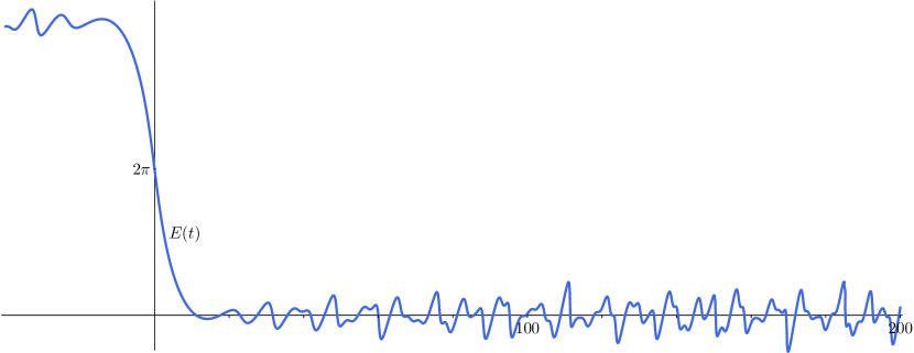
Figure 6. $E(t)$

For the next Proposition we need a measure of the possible failure of the RH.

Definition 43.

For any $t>0$ we define $\operatorname{RH}(t)$ by

(50) $$\operatorname{RH}(t):=N(t)-N_{00}(t).$$

That is $\operatorname{RH}(t)$ is equal to the number of zeros $\beta+i\gamma$ of $\zeta(s)$ with $0<\gamma\leq t$ and $\beta\neq\frac{1}{2}$, plus the number of zeros $\beta^{\prime}+i\gamma^{\prime}$ of $\zeta^{\prime}(s)$ with $\beta^{\prime}=\frac{1}{2}$ and $0<\gamma^{\prime}\leq t$ all of them counted with their multiplicities. By Proposition 10 these zeros of $\zeta^{\prime}(s)$ will be multiple zeros of $\zeta(s)$ on the critical line. We have $\operatorname{RH}(t)=0$ if and only if the zeros $\beta+i\gamma$ of $\zeta(s)$ with $0<\gamma\leq t$ are all on the critical line and are simple.

Proposition 44.

We have

(51) $$-{\textstyle\frac{1}{2}}\,+\operatorname{RH}(t)<S(t)+{\textstyle\frac{1}{\pi}}E(t)\leq{\textstyle\frac{1}{2}}\,+\operatorname{RH}(t),\qquad t>a_{\vartheta}.$$

Proof.

By (46) and (48) we have

$$S(t)+{\textstyle\frac{1}{\pi}}E(t) =N(t)-1-{\textstyle\frac{1}{\pi}}\vartheta(t)+{\textstyle\frac{1}{\pi}}\left({\textstyle\frac{3\pi}{2}}+\vartheta(t)-\pi\kappa(t)\right)$$

$$=N(t)+{\textstyle\frac{1}{2}}\,-\kappa(t)=\operatorname{RH}(t)+{\textstyle\frac{1}{2}}\,-\kappa(t)+N_{00}(t)$$

so that by (24) for $t>a_{\vartheta}$ we have

(52) $$S(t)+{\textstyle\frac{1}{\pi}}E(t)=\operatorname{RH}(t)-\left(\kappa(t)-\lfloor\kappa(t)\rfloor-{\textstyle\frac{1}{2}}\,\right),\qquad t>a_{\vartheta}$$

from which the result follows. ∎

Corollary 45.

Assuming the RH and the simplicity of the zeros we will have

(53) $$-{\textstyle\frac{1}{2}}\,<S(t)+{\textstyle\frac{1}{\pi}}E(t)\leq{\textstyle\frac{1}{2}}\,,\qquad t>a_{\vartheta}.$$

Indeed, the hypotheses are equivalent to $\operatorname{RH}(t)=0$. By the well known Fourier series of $\widetilde{B}_{1}(x)=x-\lfloor x\rfloor-\frac{1}{2}$ we get from (52), under the assumptions of the Corollary

(54) $$S(t)+{\textstyle\frac{1}{\pi}}E(t)=2\sum_{n=1}^{\infty}\frac{\sin(2\pi n\kappa(t))}{2\pi n},\qquad t>a_{\vartheta}.$$

10. Extension to other $L$-functions.

Most of the formulas and functions defined in this paper for $\zeta(s)$ can be generalized to other functions, including the Selberg class. The main thing we need is a functional equation. So let’s assume that we have a Dirichlet series

$$f(s)=\sum_{n=1}^{\infty}\frac{a_{n}}{n^{s}}$$

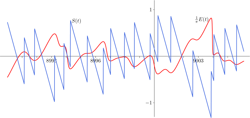
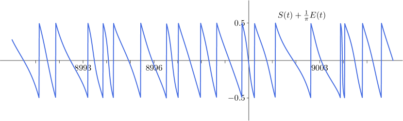
Figure 7. Plots of $S(t)$, $\frac{1}{\pi}E(t)$ and $S(t)+\frac{1}{\pi}E(t)$ for $t$ in $(8990,9006)$.

which can be extended as a meromorphic function to the plane $\mathbf{C}$, in such a way that there exist numbers $Q>0$, $\alpha_{n}>0$ and $r_{n}\in\mathbf{C}$ with $\operatorname{Re}(r_{n})\geq 0$ such that

$$\Phi(s):=Q^{s}f(s)\prod_{n=1}^{d}\Gamma(\alpha_{n}s+r_{n})\quad\text{satisfies}\quad\Phi(s)=w\overline{\Phi(1-\overline{s})}$$

where $w$ is a complex number of modulus $|w|=1$. In this way all Dirichlet series for a primitive character, and the Dirichlet series $f(s)$ considered by Titchmarsh [T]*Section 10.25, which has no Euler product, and does not satisfy an RH will be included.

Putting $s={\textstyle\frac{1}{2}}\,+it$ the functional equation leads to

$$\frac{f({\textstyle\frac{1}{2}}\,+it)}{\overline{f(\frac{1}{2}+it)}}=wQ^{-2it}\prod_{n=1}^{d}\frac{\overline{\Gamma(\alpha_{n}(\frac{1}{2}+it)+r_{n})}}{\Gamma(\alpha_{n}(\frac{1}{2}+it)+r_{n})}$$

Therefore, if we define

(55) $$\vartheta(f,t):=-\frac{\arg w}{2}+t\log Q+\sum_{n=1}^{d}\operatorname{ph}\Gamma(\alpha_{n}({\textstyle\frac{1}{2}}\,+it)+r_{n})$$

this will be a real analytic function and $\operatorname{ph}f(\frac{1}{2}+it)=-\vartheta(f,t)$ so that

(56) $$f({\textstyle\frac{1}{2}}\,+it)=e^{-i\vartheta(f,t)}Z(f,t)$$

where $Z(f,t)$ is a real valued real analytic function of the real variable $t$. It is not difficult to define functions $\kappa(f,t)$, $E(f,t)$, and so on.

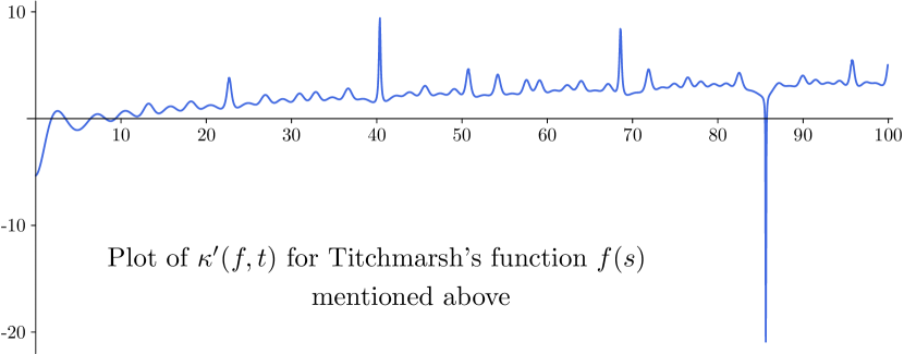
Figure 8. This Dirichlet series has a zero at the point $\rho\approx 0.80851718+i\;85.69934848$.

Acknowledgement: The authors would like to thank Patrick R. Gardner ( Kennewick, Washington, USA ) for his linguistic assistance in preparing this note, and for his interest in the subject.