Spectroscopy of a Cooper-Pair Box Coupled to a Two-Level System Via Charge and Critical Current

Abstract

We report on the quadrupling of the transition spectrum of an $\mbox{Al}/\mbox{AlO}_{x}/\mbox{Al}$ Cooper-pair box (CPB) charge qubit in the $4.0-7.3\,\mathrm{GHz}$ frequency range. The qubit was coupled to a quasi-lumped element Al superconducting resonator and measured at a temperature of $25\,\mathrm{mK}$. We obtained good matches between the observed spectrum and the spectra calculated from a model Hamiltonian containing two distinct low excitation energy two-level systems (TLS) coupled to the CPB. In our model, each TLS has a charge that tunnels between two sites in a local potential and induces a change in the CPB critical current. By fitting the model to the spectrum, we have extracted microscopic parameters of the fluctuators including the well asymmetry, tunneling rate, and a surprisingly large fractional change ($30-40\%$) in the critical current ($12\,\mathrm{nA}$). This large change is consistent with a Josephson junction with a non-uniform tunnel barrier containing a few dominant conduction channels and a TLS that modulates one of them.

Introduction

Dissipation and dephasing from two-level systems (TLS) are a serious problem in many superconducting qubits. The aggregate effect of many weakly coupled fluctuators causes $1/f$ charge noise, broadband dielectric loss, and magnetic flux noise, as well as inhomogeneous broadening and decreased measurement fidelity in qubits.Ithier et al. (2005); Simmonds et al. (2004); Martinis et al. (2005); Plourde et al. (2005); Tian and Simmonds (2007); Deppe et al. (2007) An individual TLS quantum-coherently coupled to a qubit can typically be identified when it leads to a resolvable avoided crossing in the qubit spectrum. Such avoided level crossings have been observed in phase,Cooper et al. (2004); Palomaki et al. (2010); Simmonds et al. (2004); Steffen et al. (2006) flux,Plourde et al. (2005); Deppe et al. (2007) charge,Kim et al. (2008) quantronium,Ithier et al. (2005) and transmonSchreier et al. (2008) qubits. While qubit performance is typically severely degraded near such an avoided crossing,Kim et al. (2008); Sillanpaa et al. (2007); Simmonds et al. (2004); Oh et al. (2006); Kline et al. (2009) strong qubit-TLS interactions allow the microscopic details of the TLS to be determined.Kim et al. (2008); Shalibo et al. (2010); Lupaşcu et al. (2009) Coherent coupling to a long-lived TLS also makes it possible to observe coherent oscillations between a qubit and a TLSCooper et al. (2004) or use the TLS as a quantum memory.Neeley et al. (2008); Zagoskin et al. (2006)

Two-level fluctuators in superconducting devices can be classified into three types—charge, flux, or critical current—depending on the nature of the interaction with the qubit. The microscopic origin of charge and critical current fluctuators is believed to be impurity ions such as HPaik and Osborn (2010); Phillips (1972) or low coordination bonds in the amorphous dielectric used to build the devices. In phase and flux qubits, it appears to be possible in principle but difficult in practice to identify the exact nature of the qubit-TLS interaction. In contrast, detailed spectroscopy on charge qubits or Cooper-pair boxes (CPB) has enabled the identification of discrete charge fluctuators.Kim et al. (2008) For example, Kim et al. found TLS’s that behaved as pure charge fluctuators.Kim et al. (2008) A moving charge could also modulate the critical current if it was located in the tunnel barrier.Constantin and Yu (2007) Critical current fluctuations have been frequently seen in Josephson junction devices,Clarke (1996); Savo et al. (1987); Wakai and Van Harlingen (1986) but apparently not in Josephson based qubits. This may be due to the difficulty of conclusively distinguishing a critical current fluctuator from a charge fluctuator. Alternatively, the relatively small area of qubit junctions compared to that of conventional junctions leads to far fewer total fluctuators and a corresponding decrease in the probability of observing one. Also, qubit measurements are typically made at less than $100\,\mathrm{mK}$, where critical current fluctuators appear to be frozen out. Josephson junctions are a fundamental building block of all superconducting qubits and an understanding of the origin of critical current fluctuations is important for continued improvement of qubit performance.

In this paper we report on a CPB with an unusual spectrum that has multiple spectroscopic features displaced in both frequency and in gate charge instead of an avoided level crossing. We find that the spectrum, including the curvature of the spectral features, can be modeled well with a critical current fluctuator coupled to a CPB with an excitation energy for the fluctuator much less than the qubit energy. By fitting our model to the spectrum we extract microscopic parameters for the fluctuators.

Cooper-pair Box Qubit and Readout

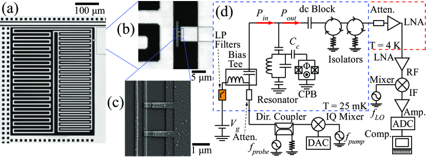
Figure 1: (a) Optical image of the lumped element resonator coupled to a CPW transmission line and surrounded by a perforated ground plane. Light regions are aluminum metalization and dark are sapphire substrate. (b) Optical image of the CPB located between the capacitor and ground plane. (c) Scanning electron image of the CPB. The twinned features are a consequence of the double-angle evaporation and the Josephson junctions are located at the overlap of the two patterns. (d) Simplified schematic of the experimental setup. The CPB is coupled through capacitor $C_{c}$ to a quasi-lumped element LC resonator. Its state is readout via a coherent heterodyne measurement of a microwave power at frequency $f_{probe}$ transmitted through the device, amplified, mixed with a local oscillator at frequency $f_{LO}$ and finally digitized. The CPB transition frequency is controlled by the gate voltage $V_{g}$ and an external magnetic flux $\Phi$ and its state is coherently manipulated using shaped microwave pulses at frequency $f_{pump}$.

Our Cooper-pair box (CPB) consists of a superconducting island connected to a superconducting reservoir (ground) through two ultrasmall Josephson tunnel junctions (critical current $I_{0}/2$ and junction capacitance $C_{j}/2$) [see Fig. 1(d)]. We can apply gate voltage $V_{g}$ to a capacitively coupled gate (capacitance $C_{g}$ to the island) to control the system’s electrostatic energy. Applying flux $\Phi$ to the loop formed by the two junctions tunes the effective total critical current $I_{0}$ via the relation $I_{0}=I_{0}^{max}\cos\left(\pi\Phi/\Phi_{0}\right)$ where $\Phi_{0}=h/2e$ is the magnetic flux quantum.

Neglecting quasiparticle states, the Hamiltonian describing a CPB in the charge basis is given byBouchiat et al. (1998)

$$\hat{H}_{CPB} = E_{c}\sum_{n}\left(2n-n_{g}\right)^{2}\left|n\right\rangle\left\langle n\right|$$ (1)

$$-\frac{E_{J}}{2}\sum_{n}\left(\left|n+1\right\rangle\left\langle n\right|+\left|n\right\rangle\left\langle n+1\right|\right)$$

where $E_{c}=e^{2}/2C_{\Sigma}$ is the charging energy, $E_{J}=I_{0}\Phi_{0}/2\pi$ is the Josephson energy, $C_{\Sigma}=C_{j}+C_{g}$ is the total island capacitance to ground, $n_{g}=C_{g}V_{g}/e$ is the reduced gate voltage and $\left|n\right\rangle$ is the excess number of Cooper-pairs on the island. For $E_{c}>E_{J}$ the system is highly anharmonic and only a few charge states are needed to accurately describe the lowest energy states. For charge qubits with $E_{c}\gg E_{J}$ and $0.5<n_{g}<1.5$, the Hamiltonian can be reduced toBouchiat et al. (1998)

$$\mathbb{H}_{CPB}=\begin{pmatrix}E_{c}\left(0-n_{g}\right)^{2}&-E_{J}/2\\ -E_{J}/2&E_{c}\left(2-n_{g}\right)^{2}\end{pmatrix}$$ (2)

which yields the excited state transition energy $\hbar\omega_{CPB}\left(n_{g}\right)=\sqrt{\left(4E_{c}\left(1-n_{g}\right)\right)^{2}+E_{J}^{2}}$. Near the charge degeneracy point $n_{g}=1$ the transition energy varies parabolically as $\hbar\omega_{CPB}\left(n_{g}\right)\approx E_{J}+8E_{c}^{2}\left(1-n_{g}\right)^{2}/E_{J}$.

To measure the state of the qubit, we coupled our qubit to a thin-film quasi-lumped element LC resonator [see Fig. 1(d)] that was in turn weakly coupled to a microwave transmission line patterned on the sample chip. To read out the state of the qubit, we apply microwave power at the resonance frequency of the resonator and record the transmitted microwave signal $S_{21}$.Gambetta et al. (2007) This is a dispersive readout in which the qubit state modulates the resonance frequency of the resonator. In the case of weak qubit-resonator coupling $g$ and large detuning $\Delta=\omega_{CPB}-\omega_{r}$ the combined CPB-resonator system Hamiltonian is approximatelyWallraff et al. (2005); Blais et al. (2004)

$$\hat{H}=\hbar\left(\omega_{r}+\frac{g^{2}}{\Delta}\sigma_{z}\right)\left(a^{\dagger}a+\frac{1}{2}\right)+\frac{\hbar\omega_{CPB}}{2}\sigma_{z}$$ (3)

where $\hbar g=\left(2E_{c}C_{c}/e\right)\sqrt{\hbar\omega_{r}/2C}$ is the strength of the qubit-resonator coupling energy, $C_{c}$ is the coupling capacitance between the resonator and the island of the CPB, $C$ is the capacitance of the LC resonator, $\omega_{r}$ is the resonance frequency, $a^{\dagger}a$ is the number operator for excitations in the resonator, and $\sigma_{z}$ is the Pauli spin operator. This Jaynes-Cummings Hamiltonian yields transitions in which the bare resonator frequency $\omega_{r}$ is dispersively shifted by $\chi=\pm g^{2}/\Delta$ depending on the state of the qubit. If $\chi<\Gamma$, where $\Gamma$ is the resonator linewidth, the average phase of the transmitted signal at $\omega=\omega_{r}$ is linearly dependent on the excited state occupation probability. On the other hand if $\chi>\Gamma$, then the in-phase or quadrature transmitted voltage is proportional to the excited state occupation probability.Gambetta et al. (2007)

Additional complications can arise when the qubit and resonator are coupled to another quantum system, such as a TLS. If multiple energy levels in the combined system have similar detunings from the resonator, the effective dispersive shift $\chi_{\mbox{eff}}$ will have a contribution from each level.Koch et al. (2007) Qubit state readout can still be performed as described for the two level case, but the sensitivity to a particular state depends on the choice of resonator probe frequency. As we see below, this is our situation.

Charge and Critical Current TLS Model

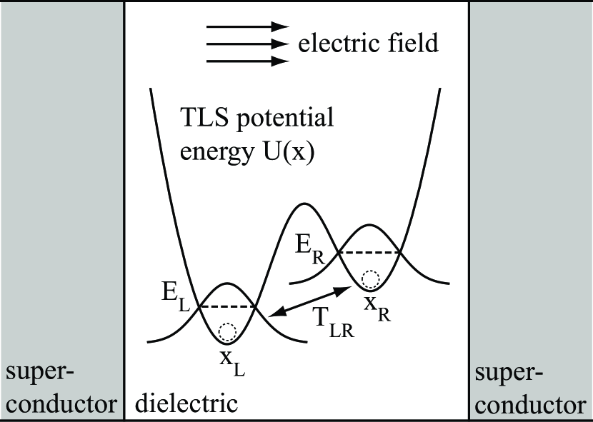
Figure 2: Simplified diagram of the potential energy of a charged TLS in an insulating tunnel barrier. The fluctuator can be localized at positions $x_{R}$ or $x_{L}$ with corresponding energies $E_{R}$ or $E_{L}$ and can tunnel between them with energy $T_{LR}$. Additionally the Josephson energy $E_{J}$ of the CPB depends on whether the fluctuator is at $x_{R}$ or $x_{L}$.

To include the effects on a CPB produced by a combined charge and critical current fluctuator, we expand on the charge defect model previously reported by Z. Kim, et al.Kim et al. (2008); Wellstood et al. (2008) We assume the fluctuator acts as a two-level system in which a point charge in the tunnel barrier can tunnel between two potential well minima. In the TLS position basis the fluctuator Hamiltonian is given by

$$\mathbb{H}_{TLS}=\begin{pmatrix}E_{L}&T_{LR}\\ T_{LR}&E_{R}\end{pmatrix}$$ (4)

where $E_{L}$ and $E_{R}$ are energies of the charge in the left and right position states and $T_{LR}$ is the tunneling matrix element [see Fig. 2]. For an isolated fluctuator the excited state transition energy is given by $\hbar\omega_{TLS}=\sqrt{\left(E_{R}-E_{L}\right)^{2}+4T_{LR}^{2}}$.

The charge coupling between the CPB and TLS originates from changes in the electrostatic potential when the defect tunnels between its two sites. Using Green’s reciprocation theoremJackson (1999) the change in the induced polarization charge on the island of the CPB when the fluctuator tunnels from the left to the right well is $\Delta Q_{pi}=Q_{TLS}\left(x_{R}-x_{L}\right)\cos\left(\eta\right)/d$ where $Q_{TLS}$ is the TLS charge, $\eta$ is the angle the TLS displacement vector makes relative to the electric field in the junction and $d\approx 1\,\mathrm{nm}$ is the thickness of the tunnel junction. For fixed net charge on the island this in turn results in a change in the electrostatic potential of the island given by

$$\Delta V_{i}=\frac{Q_{TLS}}{C_{\Sigma}}\frac{\left(x_{R}-x_{L}\right)\cos\left(\eta\right)}{d}\mbox{.}$$ (5)

Accounting for the electrostatic charging energy and the work done by the gate voltage source when the point charge moves, the coupling Hamiltonian is given by

$$\hat{H}_{CPB-TLS}=2E_{c}\left(2\hat{N}-n_{g}\right)\frac{Q_{TLS}}{e}\frac{\hat{x}\cos\left(\eta\right)}{d}$$ (6)

where $\hat{N}$ is the CPB charge operator that counts the number of excess Cooper-pairs on the island and $\hat{x}$ is the TLS position operator.Wellstood et al. (2008)

Combining Eqs. (2), (4) and (6) we can write the total Hamiltonian for a CPB coupled to a single charge fluctuator as $\hat{H}=\hat{H}_{CPB}+\hat{H}_{TLS}+\hat{H}_{CPB-TLS}$. In block matrix form this becomes

$$\mathbb{H}=\begin{pmatrix}\mathbb{H}_{L}&\mathbb{T}\\ \mathbb{T}&\mathbb{H}_{R}\end{pmatrix}$$ (7)

where $\mathbb{T}=T_{LR}\mathbb{I}$, $\mathbb{I}$ is the $2\times 2$ identity matrix, and $\mathbb{H}_{L}$ and $\mathbb{H}_{R}$ are the CPB Hamiltonian with the TLS in either the left or right well. If we assume $E_{L}=0$ then $\mathbb{H}_{L}=\mathbb{H}_{CPB}$ as given by Eq. (2) and

$$\mathbb{H}_{R}=\begin{pmatrix}E_{c}\left(0-n_{g}\right)^{2}+E_{int}\left(0-n_{g}\right)+E_{R}&-E_{J}/2\\ -E_{J}/2&E_{c}\left(2-n_{g}\right)^{2}+E_{int}\left(2-n_{g}\right)+E_{R}\end{pmatrix}$$ (8)

where $E_{int}=2E_{c}Q_{TLS}\left(x_{R}-x_{L}\right)\cos\left(\eta\right)/ed$ sets the energy scale for the charge coupled interaction between the fluctuator and the CPB.

If the TLS is in the junction tunnel barrier, it can also modulate the critical current depending on its position.Constantin and Yu (2007) This coupling can be accounted for by making the substitution $E_{J}\rightarrow E_{J}+\Delta E_{J}/2$ in $\mathbb{H}_{L}$ and $E_{J}\rightarrow E_{J}-\Delta E_{J}/2$ in $\mathbb{H}_{R}$.

Numerically diagonalizing the resulting $4\times 4$ Hamiltonian $\mathbb{H}$, we find the energy levels and the transition frequencies from the ground state to the excited states of the system. An avoided crossing occurs if the excited state of the TLS is resonant with the first excited state of the CPB at some value of the gate voltage $n_{g}$.Kim et al. (2008); Wellstood et al. (2008) However if the TLS excited state energy lies below the CPB transition minimum the CPB spectrum is twinned, with one parabola corresponding primarily to the excited state of the CPB and the other to a joint excitation of the CPB and the TLS. Considered individually, each parabola bears a strong resemblance to the spectrum of a TLS-free CPB. When the tunneling energy $T_{LR}$ is small we can identify the qualitative effects of each parameter on the twinned parabolas. $\Delta E_{J}$ creates an offset along the frequency axis and a change in the effective curvature while $E_{int}$ creates an offset along the $n_{g}$ axis and “tilts” the parabolas. $E_{R}$ also creates an offset along the frequency axis that adds to or subtracts from the effect of $\Delta E_{J}$. Finally $T_{LR}$ determines the size of any avoided crossings that are present in the spectrum and determines the transition rate induced by a gate perturbation between the ground state and excited states involving the TLS.

We can further extend the model by considering the effect of two critical current fluctuators. This is motivated by the observation of quadrupling of the spectral lines in our data which can’t be explained by the presence of a single TLS. The total Hamiltonian for a CPB coupled to two fluctuators in block matrix form is

$$\mathbb{H}=\begin{pmatrix}\mathbb{H}_{LL}&\mathbb{T}_{1}&\mathbb{T}_{2}&\mathbb{T}_{12}\\ \mathbb{T}_{1}&\mathbb{H}_{RL}&\mathbb{T}_{12}&\mathbb{T}_{2}\\ \mathbb{T}_{2}&\mathbb{T}_{12}&\mathbb{H}_{LR}&\mathbb{T}_{1}\\ \mathbb{T}_{12}&\mathbb{T}_{2}&\mathbb{T}_{1}&\mathbb{H}_{RR}\end{pmatrix}$$ (9)

where $\mathbb{T}_{1}=T_{LR,1}\mathbb{I}$, $\mathbb{T}_{2}=T_{LR,2}\mathbb{I}$, and $\mathbb{T}_{12}=T_{12}\mathbb{I}$ where $T_{12}$ accounts for any possible TLS-TLS coupling and the indices refer to the first or second TLS. $\mathbb{H}_{ij}$ with $i,j\in\left\{L,R\right\}$ is the CPB Hamiltonian with the respective TLS in either the left or right well. For example, $\mathbb{H}_{RL}$ is given by

$$\mathbb{H}_{RL}=\begin{pmatrix}E_{c}\left(0-n_{g}\right)^{2}+E_{int,1}\left(0-n_{g}\right)+E_{R,1}&-\left(E_{J}-\Delta E_{J,1}/2+\Delta E_{J,2}/2\right)/2\\ -\left(E_{J}-\Delta E_{J,1}/2+\Delta E_{J,2}/2\right)/2&E_{c}\left(2-n_{g}\right)^{2}+E_{int,1}\left(2-n_{g}\right)+E_{R,1}\end{pmatrix}$$ (10)

and $\mathbb{H}_{LR}$ has the respective indices swapped. $\mathbb{H}_{RR}$ includes the contribution of both TLS and in addition present on the diagonal is a CPB mediated TLS-TLS interaction termWellstood et al. (2008) of the form $E_{int,1}E_{int,2}/2E_{c}$.

Experimental Details

We fabricated a thin-film lumped-element superconducting microwave resonator using standard photolithography and lift-off techniques. It was made from a $100\,\mathrm{nm}$ thick film of thermally evaporated Al on a c-plane sapphire wafer that was patterned into a meander inductor ($L\approx 2\,\mathrm{nH}$) and interdigital capacitor ($C\approx 400\,\mathrm{fF}$) coupled to a coplanar waveguide transmission line [see Fig. 1(a,b)]. The resonance frequency was $\omega_{r}/2\pi=5.47\,\mathrm{GHz}$ with loaded quality factor $Q_{L}=35,000$, external quality factor $Q_{e}=47,000$, and internal quality factor $Q_{i}=147,000$.

The CPB was subsequently defined by e-beam lithography and deposited using double-angle evaporation and thermal oxidation of aluminum to create the $350\,\mathrm{nm}\times 150\,\mathrm{nm}$ Josephson tunnel junctions [see Fig. 1(c)].Dolan (1977) For the e-beam lithography we used a bilayer stack of MMA(8.5)MAA copolymer and ZEP520A e-beam resist to facilitate lift-off and reduce proximity exposure during writing. A $30\,\mathrm{nm}$ thick Al island and $50\,\mathrm{nm}$ thick Al leads were deposited in an e-beam evaporator. As discussed below, measurements of the CPB yielded $E_{c}/h$ in the $4.4-5.3\,\mathrm{GHz}$ range and we tuned $E_{J}/h$ from $4\,\mathrm{GHz}$ to $E_{J}^{max}/h=7.33\,\mathrm{GHz}$.

The chip was enclosed in a rf-tight Cu box that was anchored to the mixing chamber of an Oxford Instruments model 100 dilution refrigerator at $25\,\mathrm{mK}$. Connections to the chip were made with Al wirebonds. We used cold attenuators on the input microwave line and isolators on the output line to filter thermal noise from higher temperatures [see Fig. 1(d)]. A filtered dc bias voltage line was coupled to the input line using a bias tee before the device and a dc block was placed after the sample box.

For spectroscopic measurements the resonator was probed with a weak continuous microwave signal while a second pump tone was applied to excite the qubit. The transmitted microwave signal at the probe frequency was amplified with a HEMT amplifier sitting in the He bath [see Fig. 1(d)]. We implemented a coherent heterodyne setup to record the phase and amplitude of the transmitted probe signal at $500\,\mathrm{ns}$ time steps. After the HEMT, the signal was further amplified at room temperature, mixed with a local oscillator tone to an intermediate frequency of $2\,\mathrm{MHz}$ and then digitally sampled at a typical sampling rate of $20\,\mathrm{MSa/s}$. A reference tone split off from the probe signal was directly mixed and digitally sampled. Both signals passed though a second stage of digital demodulation on a computer to extract the amplitude and phase. All components were locked to a $10\,\mathrm{MHz}$ Rb atomic clock. Both the probe and pump tone powers were optimized for ease of data acquisition while also minimally disturbing the qubit. The probe tone power was calibrated via the ac Stark shift.Schuster et al. (2005) During measurement of the qubit state, the probe tone power was set to populate the resonator with an average $\bar{n}=25$ photons while the concurrent pump tone power was slightly above that needed to saturate the CPB transitions.

Spectrum Characterization

We measured the transition spectrum of the qubit by recording the transmitted microwave probe signal while sweeping the dc gate voltage and stepping the frequency of the second microwave pump signal. Fig. 4(d) shows a plot of the transmitted probe signal amplitude as functions of $n_{g}$ and pump frequency $f_{pump}$ with $E_{J}$ tuned near $E_{J}^{max}$. Several unexpected and anomalous features are evident. Rather than a single parabola, we observed two parabolas with varying curvatures offset by $\approx 0.25\,\mathrm{GHz}$ in frequency and $\approx 0.04e$ in charge. This spectral structure was stable over the course of four months and persisted as we tuned the transition frequency from $4.0-7.3\,\mathrm{GHz}$. Close examination of the figure reveals sections of two more quite weak parabolas. A notable change in the spectrum occurred when we tuned $E_{J}$ to bring the transition frequency below that of the resonator. As seen in Fig. 4(a), four parabolas are clearly visible with the stronger new pair displaced $\approx 0.40\,\mathrm{GHz}$ below the original two. We note two additional anomalies we observed. First, a “dead zone” was present between $\approx 5.6-6.5\,\mathrm{GHz}$ where no spectrum was visible. Second, only half of the spectral parabolas—one from each pair—were visible when measured with a pulsed probe readout. For instance, in Fig. 4(d) both parabolas were present when we used a continuous measurement but only the bottom parabola was visible when we used a pulsed measurement at a fixed gate voltage $n_{g}=1$.

Some clues about the nature of the fluctuator are evident from an examination of the spectrum. The frequency offset between the two parabolas in Fig. 4(d) could be caused by a flux fluctuator that modulates $E_{J}$. However such a fluctuator’s effect on $E_{J}\left(\Phi\right)$ would be minimal when the applied flux is near zero and increase as $E_{J}$ is reduced by an external flux bias. As discussed below, this is the opposite of the behavior we observed. Another argument against a simple flux fluctuator (such as a vortex) or a simple charge fluctuator is that there are correlated shifts in $n_{g}$ and frequency between the parabolas. In contrast, the observed offsets and curvature changes are consistent with a two-level system that is coupled to the CPB via both charge and critical current.

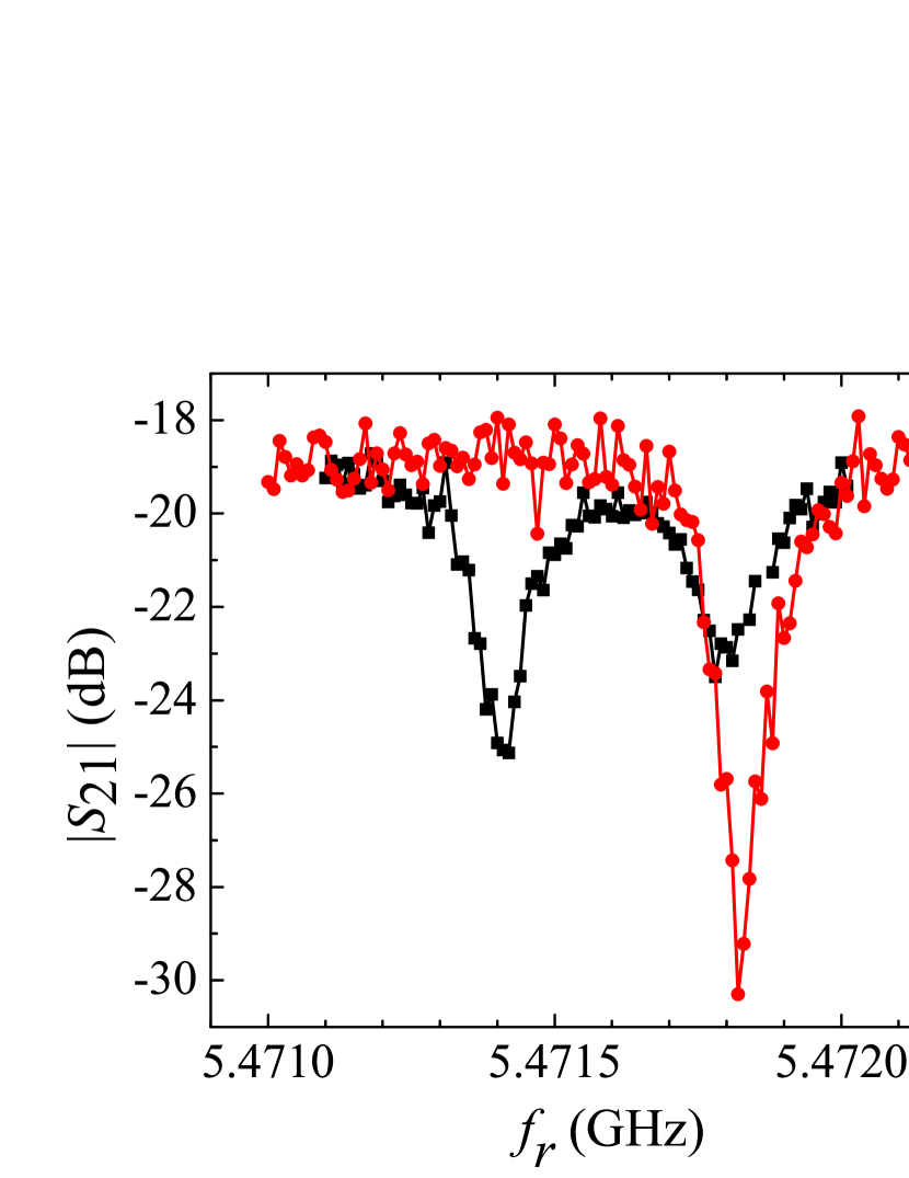
Figure 3: Plot of the ratio of the transmitted output voltage to input voltage ($\left|S_{21}\right|$) versus frequency for two different preparations of the qubit state. The filled black squares and black curve show the transmission with the qubit biased at $n_{g}=1$ and driven to a mixed ground and excited state. The two dips are resonances at $\omega_{r}^{\prime}\pm\chi_{\mbox{eff}}$. The filled red circles and red curve show the transmission with the qubit in the ground state and far detuned from the resonator at $n_{g}=0$. The single dip is the bare resonator frequency at $\omega_{r}$ .

Several factors indicate that the fluctuator is coherently coupled to the CPB. An incoherently coupled low frequency critical current fluctuator would be expected to produce twinning in the resonator dispersive shift $\chi$ in addition to twinning of the spectral lines. This twinning of the dispersive shift would be manifest either as twinning of the ground state resonator frequency or broadening of the resonator linewidth. We didn’t observe either of these effects. Instead we observed an effective dispersive shift $\chi_{\text{eff}}$ consistent with contributions from multiple levels [see Fig. 3]. We determined the effective dispersive shift $\chi_{\text{eff}}$ and effective resonator frequency $\omega_{r}^{\prime}$ by recording the resonator response with the qubit in the ground and excited states. We also measured the bare resonator frequency $\omega_{r}$ by far detuning the qubit from the resonator by biasing at $n_{g}=0$ [see Fig. 3]. As expected $\omega_{r}^{\prime}\neq\omega_{r}$ and the effective dispersive shift $\chi_{\text{eff}}$ differed between the excited states corresponding to the various parabolas. Finally, in previous cases of incoherent fluctuator coupling we found that the qubit was rendered inoperable.Schuster (2007); Kim (2010) Yet in this case we were able to measure qubit excited state lifetimes $T_{1}$ in the $15-30\,\mathrm{\text{\leavevmode{m}}s}$ range and record Rabi oscillations for all of the parabolas.

The strength of the qubit-TLS coupling indicates that the TLS was located close to the CPB Josephson junctions, either in the tunnel barrier itself or on the surface of the CPB island. Furthermore, we note that the spectra were $2e$ periodic in $n_{g}$. This is the expected periodicity for a charge fluctuator that is in the tunnel barrierWellstood et al. (2008), and such a fluctuator would need to be in the $\mbox{AlO}_{x}$ tunnel barrier to produce a critical current change.

Fitting and Discussion

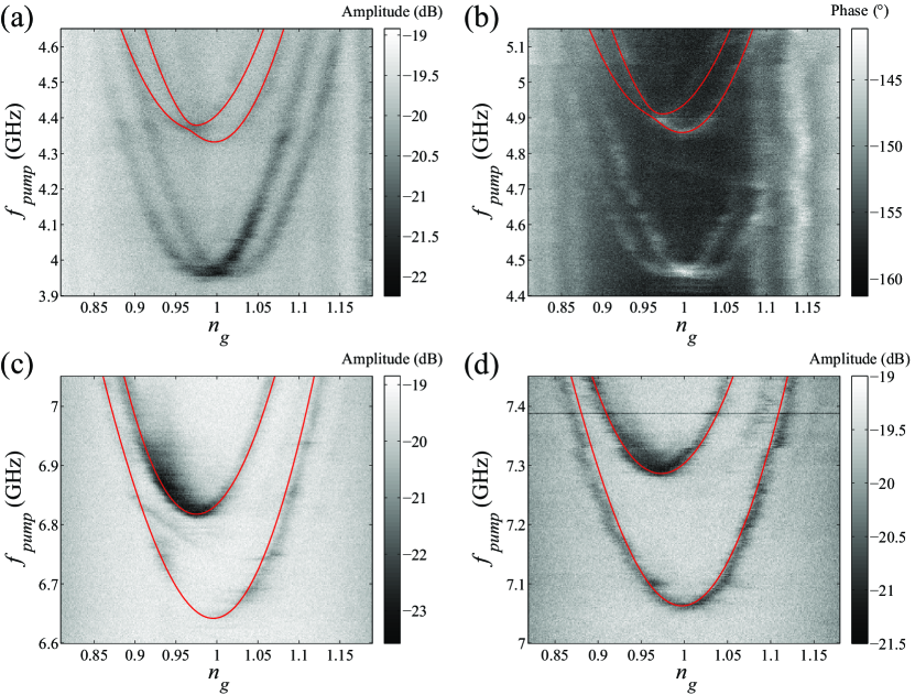
Figure 4: Measured transition spectrum of the CPB at four different external magnetic flux $\Phi$ bias values. The red lines are the theoretical spectrum using a Hamiltonian consisting of a single charged two-level fluctuator coupled to a CPB. In (a) and (b) (data sets #1 and #2) the qubit transition frequency is tuned below the resonator and only the top two parabolas were considered when fitting to the model. In (c) and (d) (data sets #3 and #4) the qubit transition frequency is tuned above the resonator. Table 1 lists the parameters used to generate each curve. (d) The dark horizontal line at $7.39\,\mathrm{GHz}$ is a charge noise artifact.

Table 1: Fit parameters for the model of a single two-level fluctuator coupled to a CPB. The corresponding spectra are plotted in Fig. 4. $E_{c}$ and $E_{J}$ are the CPB charging and Josephson energies. $E_{R}$ is the TLS potential energy well asymmetry, $E_{int}$ is the charge coupling between the TLS and the CPB, $\Delta E_{J}$ is the change in the CPB Josephson energy when the TLS tunnels between wells and $T_{LR}$ is the TLS tunneling rate.

Data set		#1		#2		#3		#4
$E_{c}/h$ (GHz)		$4.5$		$4.5$		$4.5$		$4.5$
$E_{J}/h$ (GHz)		$3.64$		$4.16$		$5.93$		$6.33$
$\Delta E_{J}/h$ (GHz)		$1.50$		$1.54$		$1.84$		$2.02$
$E_{R}/h$ (GHz)		$0.62$		$0.62$		$0.62$		$0.62$
$E_{int}/h$ (GHz)		$0.35$		$0.35$		$0.35$		$0.35$
$T_{LR}/h$ (GHz)		$0.01$		$0.01$		$0.06$		$0.06$

We first fit the single TLS model to the measured spectrum at several different external flux bias values. In our device $E_{c}$ is comparable to $E_{J}$, so we needed to include $4$ charge states in the CPB Hamiltonian block matrices to better approximate the CPB behavior. We initially focused only on the top two parabolas to better understand the effects of the model parameters and the relation between the one and two TLS models. The solid red curves in Fig. 4 show the predicted spectrum for those parabolas and the fits look reasonable.

The optimal fit parameters are summarized in Table 1 and give reasonable results for all values of the flux bias. Individual fit parameters could typically be varied by approximately 20% while maintaining a reasonable looking fit. The large uncertainty is partly due to the fact that the frequency offset between the twinned parabolas arises from both $\Delta E_{J}$ and $E_{R}$. Additionally the model predicts avoided crossings which were too small to resolve, and this meant we could place an upper bound on the TLS tunneling strength $T_{LR}$. We note that the data sets with different applied flux only require $E_{J}$ and $\Delta E_{J}$ to be adjusted, which is consistent with changing flux bias, except for a change in $T_{LR}$ when the qubit is tuned from below to above the resonator $\omega_{r}$. The model also predicts a nearly flat TLS spectral line in the $1-2\,\mathrm{GHz}$ range, roughly equal to the transition frequency of the isolated fluctuator. We didn’t observe such a feature, perhaps because our resonator perturbative measurement technique was insensitive to a low frequency TLS-only transition.

It is important to consider if other models can explain our observations. We can eliminate a coherently coupled flux fluctuator using the same reasoning used to exclude the incoherently coupled case. In particular this suggests that the unusual spectrum isn’t due to coupling to a moving vortex. Another possibility is that the data could be fit by a charged fluctuator with $\Delta E_{J}=0$. Such model would predict a large “tilt” of the parabolas that disagrees with data covering a wider $n_{g}$ and frequency span.

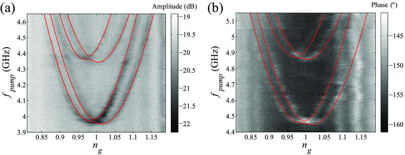
Figure 5: Measured transition spectrum of the CPB at two different external magnetic flux $\Phi$ bias values. The red lines are the theoretical spectrum using a Hamiltonian consisting of two charged two-level fluctuators coupled to a CPB. Plots (a) and (b) (data sets #1 and #2) are the same data sets as plots (a) and (b) in Fig. 4. Table 2 lists the parameters used to generate each curve.

Table 2: Fit parameters for the model of two two-level fluctuators coupled to a CPB. The corresponding spectra are plotted in Fig. 5. $E_{c}$ and $E_{J}$ are the CPB charging and Josephson energies. $E_{R,1}$ and $E_{R,2}$ are the potential energy well asymmetries for the first and second TLS. Similarly $E_{int,1}$ and $E_{int,2}$ are the charge coupling between the first and the second TLS and the CPB and $\Delta E_{J,1}$ and $\Delta E_{J,2}$ are the changes in the CPB Josephson energy when the TLS tunnel between their respective wells. $T_{LR,1}$ and $T_{LR,2}$ are the TLS tunneling rates while $T_{12}$ is the TLS-TLS coupling strength.

Data set		#1		#2
$E_{c}/h$ (GHz)		$4.3$		$4.3$
$E_{J}/h$ (GHz)		$2.79$		$3.43$
$\Delta E_{J,1}/h$ (GHz)		$1.36$		$1.40$
$E_{R,1}/h$ (GHz)		$0.62$		$0.62$
$E_{int,1}/h$ (GHz)		$-0.40$		$-0.40$
$T_{LR,1}/h$ (GHz)		$0.00$		$0.00$
$\Delta E_{J,2}/h$ (GHz)		$-1.00$		$-0.68$
$E_{R,2}/h$ (GHz)		$-0.82$		$-0.69$
$E_{int,2}/h$ (GHz)		$0.13$		$0.15$
$T_{LR,2}/h$ (GHz)		$0.04$		$0.04$
$T_{12}/h$ (GHz)		$0.04$		$0.04$

We also fit the entire spectrum of four parabolas to the two TLS model [see Eqs. 9 and 10]. The solid red curves in Fig. 5 show the best fit spectrum superposed on the data. The optimal fit parameters are summarized in Table 2. The vertical lines at $n_{g}\approx 1\pm 0.09$ and $n_{g}\approx 1\pm 0.14$ are due to the resonant crossing between the qubit parabolas and the resonator line at $\omega_{r}$. Although the fits are reasonable and capture all of the major features, the fit parameters contain one surprise. If we assume two independent fluctuators, the simplest assumption in light of the strong shielding of electric fields in the dielectric of the Josephson junction by the superconducting electrodes, then we would expect $T_{LR,1}\neq 0$ and $T_{LR,2}\neq 0$ while $T_{12}=0$. However our fit yields $T_{LR,1}=0$ while $T_{LR,2}\neq 0$ and $T_{12}\neq 0$ which suggests coupled TLS’s or more complicated microscopic behavior. Furthermore, we note that several of the TLS parameters, such as the charge coupling $E_{int,1}$, change values when switching from the single to the double TLS model. This indicates that the two TLS model is needed to explain the full quadrupled spectrum and suggests that there is significant interaction between the TLS’s.

There are some noteworthy implications from the magnitude of the fit parameters. First, we note that $\Delta E_{J}/E_{J}\approx 30\%$. The large relative size of $\Delta E_{J}$ to $E_{J}$ suggests that the junction tunnel barrier is non-uniform with a few dominant conduction channels and that the TLS is located near and modulates one of these channels.Dorneles et al. (2003) Second, the TLS tunneling matrix element $T_{LR}\lesssim 0.06\,\mathrm{GHz}$ is small compared to the other energies in the system, indicating that the TLS is tunneling between fairly well isolated sites. We can also place a lower bound on $T_{LR}$ by noting that for $T_{LR}<0.01\,\mathrm{GHz}$ the spectra would be too faint to observe. If the excited state of such a TLS were resonant with the first excited state of the CPB, the resulting avoided crossing would be very small and difficult to resolve. Our extracted tunneling matrix element values are also significantly smaller than those reported by Z. Kim, et al.,Kim et al. (2008) which were in the $3-13\,\mathrm{GHz}$ range. There is a similar relation between the range of well asymmetry values extracted by us, $E_{R}=0.6-0.8\,\mathrm{GHz}$, and those reported by Z. Kim, et al., $E_{R}=7-39\,\mathrm{GHz}$. Assuming a TLS charge of $Q_{TLS}=e$ and a tunnel barrier thickness of $d=1\,\mathrm{nm}$, we estimate the maximum hopping distance of the defect at $0.2-0.45$ Å. This is in agreement with the bounds of $0.32-0.83$ Å found by Z. Kim, et al.

Discrete critical current fluctuators have been reported in current biased Josephson junctions, identified via either a random telegraph signal in the voltage time trace or a signature Lorentzian bump in the noise spectrum.Eroms et al. (2006); Gustafsson et al. (2011); Savo et al. (1987); Wakai and Van Harlingen (1986) One way we can compare our TLS’s to others is to calculate the effective defect area $A_{\text{eff}}$ given by $A_{\text{eff}}=\left(\Delta E_{J}/E_{J}\right)A_{j}$. For our device find $A_{\text{eff}}\approx 18,000\,\mathrm{nm^{2}}$ where $A_{j}=350\times 150\,\mathrm{nm^{2}}$ is the junction area. This value is much larger than the $A_{\text{eff}}=1-2\,\mathrm{nm^{2}}$ reported in similar junctions,Eroms et al. (2006) the $A_{\text{eff}}\approx 600\,\mathrm{nm^{2}}$ seen in larger area junctions,Savo et al. (1987) or the $A_{\text{eff}}=72\,\mathrm{nm^{2}}$ found in similar area $\mbox{high-}T_{c}$ superconductor grain boundary junctions.Gustafsson et al. (2011) On the other hand, the absolute value of the critical current fluctuation $\Delta I_{0}\approx 4\,\mathrm{nA}$ we observed is close to that reported in both similar area ($\Delta I_{0}=9.2\,\mathrm{nA}$)Wakai and Van Harlingen (1986) and larger junctions ($\Delta I_{0}\approx 1\,\mathrm{nA}$).Savo et al. (1987) One notable difference that might account for some of these discrepancies is that the critical current density of our sample ($23\,\mathrm{A/cm^{2}}$) is smaller by an order of magnitude or more than the referenced samples. If we assume that the conductance of a tunneling channel is similar between the various devices, this is consistent with a small number of tunneling hot spots in our junction.

Comments and Conclusion

The longitudinal relaxation rate of a TLS in an amorphous solid is expected to be limited by $1/T_{1}=\alpha\hbar\omega_{TLS}T_{LR}^{2}\coth\left(\hbar\omega_{TLS}/2k_{B}T\right)$ where $T$ is temperature and $\alpha$ is a material dependent constant.Phillips (1981) From the results of Z. Kim, et al.Kim et al. (2008) we estimate $1/\alpha\approx 10^{2}\,\mathrm{\text{\leavevmode{m}}s\cdot GHz^{3}}\cdot h^{3}$ for the dielectric $\mbox{AlO}_{x}$ in the tunnel junction barrier. Our fit values then place an upper bound on the TLS excited state lifetime of $T_{1}\lesssim 1\,\mathrm{ms}$. This bound is consistent with a relatively long TLS lifetime and with our qubit $T_{1}\approx 15-30\,\mathrm{\text{\leavevmode{m}}s}$. The excited states of the system are mixtures of pure CPB and TLS excited states, so the decay rate is a weighted average of the pure CPB and TLS decay rates. For example, according to our fits to the model at $n_{g}=1$ the lower parabola in Fig. 4(d) is composed of a $12\%$ CPB excitation and an $88\%$ joint CPB plus TLS excitation while the upper parabola is an $88\%$ CPB excitation and a $12\%$ joint CPB plus TLS excitation. Only when both the qubit and TLS decay rates are small, as is our case, will the system decay time be long in both parabolas.

Finally it’s worthwhile to speculate why this behavior was observed in our sample. In order to observe spectral twinning rather than an avoided crossing, the TLS needs to be coupled to the qubit but have a transition frequency less than $E_{J}/h$. That this occurred is a statistical coincidence. Observing two such defects in the same sample is less likely, and the TLS fit parameters suggest they are correlated. Furthermore, we are biased in selecting samples for detailed study that have especially conspicuous features, such as large avoided crossings or anomalous spectra, and the parameter values of such samples are likely to be somewhat unusual.

While our simple model provides a good fit to the recorded spectrum, it leaves other questions unanswered. The resonator wasn’t included in the model but some of our observations suggest that it may produce significant effects on the spectrum. Inclusion of the resonator in the model would allow a theoretical calculation of the expected dispersive shift and a comparison with the data. A more complete model may also elucidate the role, if any, the resonator played in the the large difference in the visibility of the different parabolas when the qubit was tuned from below to above the resonator $\omega_{r}$ or the “dead zone” we observed between $\approx 5.6-6.5\,\mathrm{GHz}$ where no spectrum was visible. Perhaps the most puzzling feature was that half of the spectral parabolas weren’t visible when measured with a pulsed probe. Unfortunately additional data on this issue wasn’t obtained.

In conclusion we have examined the transition spectrum of a CPB that had an anomalous quadrupling of the spectral lines. A microscopic model of one or two charged critical current fluctuators coupled to a CPB was used to fit the spectrum. The fits were in good agreement with the data, reproduced the key features in the spectrum, and allowed us to extract microscopic parameters for the TLS’s. Our tunneling terms were much smaller than those reported by Z. Kim, et al.Kim et al. (2008) in their measurements of avoided crossings. Finally, the large fractional change $\Delta E_{J}/E_{J}$ of $30-40\%$ suggests that the tunnel barrier is non-uniform in thickness with the TLS hopping blocking a dominant conduction channel.