An Efficient Parallel Immersed Boundary Algorithm using a Pseudo-Compressible Fluid Solver

Abstract

We propose an efficient algorithm for the immersed boundary method on distributed-memory architectures that has the computational complexity of a completely explicit method and also has excellent parallel scaling. The algorithm utilizes the pseudo-compressibility method recently proposed by Guermond and Minev that uses a directional splitting strategy to discretize the incompressible Navier-Stokes equations, thereby reducing the linear systems to a series of one-dimensional tridiagonal systems. We perform numerical simulations of several fluid-structure interaction problems in two and three dimensions and study the accuracy and convergence rates of the proposed algorithm. We also compare the proposed algorithm with other second-order projection-based fluid solvers. Lastly, the execution time and scaling properties of the proposed algorithm are investigated and compared to alternate approaches.

url]http://www.jkwiens.com/ url]http://www.math.sfu.ca/ stockie

1 Introduction

The immersed boundary (IB) method is a mathematical framework for studying fluid-structure interaction that was originally developed by Peskin to simulate the flow of blood through a heart valve [49]. The IB method has been used in a wide variety of biofluids applications including blood flow through heart valves [26, 49], aerodynamics of the vocal cords [14], sperm motility [12], insect flight [41], and jellyfish feeding dynamics [32]. The method is also increasingly being applied in non-biological applications [43].

The immersed boundary equations capture the dynamics of both fluid and immersed elastic structure using a mixture of Eulerian and Lagrangian variables: the fluid is represented using Eulerian coordinates that are fixed in space, and the immersed boundary is described by a set of moving Lagrangian coordinates. An essential component of the model is the Dirac delta function that mediates interactions between fluid and IB quantities in two ways. First of all, the immersed boundary exerts an elastic force (possibly singular) on the fluid through an external forcing term in the Navier-Stokes equations that is calculated using the current IB configuration. Secondly, the immersed boundary is constrained to move at the same velocity as the surrounding fluid, which is just the no-slip condition. The greatest advantage of this approach is that when the governing equations are discretized, no boundary-fitted coordinates are required to handle the solid structure and the influence of the immersed boundary on the fluid is captured solely through an external body force.

When devising a numerical method for solving the IB equations, a common approach is to use a fractional-step scheme in which the fluid is decoupled from the immersed boundary, thereby reducing the overall complexity of the method. Typically, these fractional-step schemes employ some permutation of the following steps:

• Velocity interpolation: the fluid velocity is interpolated onto the immersed boundary.

• IB evolution: the immersed boundary is evolved in time using the interpolated velocity field.

• Force spreading: calculate the force exerted by the immersed boundary and spreads it onto the nearby fluid grid points, with the resulting force appearing as an external forcing term in the Navier-Stokes equations.

• Fluid solve: evolve the fluid variables in time using the external force calculated in the force spreading step.

Algorithms that fall into this category include Peskin’s original method [49] as well as algorithms developed by Lai and Peskin [36], Griffith and Peskin [27], and many others.

A popular recent implementation of fractional-step type is the IBAMR code [35] that supports distributed-memory parallelism and adaptive mesh refinement. This project grew out of Griffith’s doctoral thesis [21] and was outlined in the papers [24, 27]. In the original IBAMR algorithm, the incompressible Navier-Stokes equations are solved using a second-order accurate projection scheme in which the viscous term is handled with an L-stable discretization [40, 61] while an explicit second-order Godunov scheme [11, 42] is applied to the nonlinear advection terms. The IB evolution equation is then integrated in time using a strong stability-preserving Runge-Kutta method [20]. Since IBAMR’s release, drastic improvements have been made that increase both the accuracy and generality of the software [23, 26].

Fractional-step schemes often suffer from a severe time step restriction due to numerical stiffness that arises from an explicit treatment of the immersed boundary in the most commonly used splitting approaches [58]. Because of this limitation, many researchers have proposed new algorithms that couple the fluid and immersed boundary together in an implicit fashion, for example [8, 34, 37, 44, 47]. These methods alleviate the severe time step restriction, but do so at the expense of solving large nonlinear systems of algebraic equations in each time step. Although these implicit schemes have been shown in some cases to be competitive with their explicit counterparts [48], there is not yet sufficient evidence to prefer one approach over the other, especially when considering parallel implementations.

Projection methods are a common class of fractional-step schemes for solving the incompressible Navier-Stokes equations, and are divided into two steps. First, the discretized momentum equations are integrated in time to obtain an intermediate velocity field that in general is not divergence-free. In the second step, the intermediate velocity is projected onto the space of divergence-free fields using the Hodge decomposition. The projection step typically requires the solution of large linear systems in each time step that are computationally costly and form a significant bottleneck in CFD codes. This cost is increased even more when a small time step is required for explicit implementations. Note that even though some researchers make use of unsplit discretizations of the Navier-Stokes equations [23, 48], there is significant benefit to be had by using a split-step projection method as a preconditioner [22]. Therefore, any improvements made to a multi-step fluid solver can reasonably be incorporated into unsplit schemes as well.

In this paper, we develop a fractional-step IB method that has the computational complexity of a completely explicit method and exhibits excellent parallel scaling on distributed-memory architectures. This is achieved by abandoning the projection method paradigm and instead adopting the pseudo-compressible fluid solver developed by Guermond and Minev [28, 29]. Pseudo-compressibility methods relax the incompressibility constraint by perturbing it in an appropriate manner, such as in Temam’s penalty method [59], the artificial compressibility method [9], and Chorin’s projection method [10, 53]. Guermond and Minev’s algorithm differentiates itself by employing a directional-splitting strategy, thereby permitting the linear systems of size $N^{d}\times N^{d}$ typically arising in projection methods (where $d=2$ or 3 is the problem dimension) to be replaced with a set of one-dimensional tridiagonal systems of size $N\times N$. These tridiagonal systems can be solved efficiently on distributed-memory computing architectures by combining Thomas’s algorithm with a Schur-complement technique. This allows the proposed IB algorithm to efficiently utilize parallel resources [18]. The only serious limitation of the IB algorithm is that it is restricted to simple geometries and boundary conditions due to the directional-splitting strategy adopted by Guermond and Minev. However, since IB practitioners often use a rectangular fluid domain with periodic boundary conditions, this is not a serious limitation. Instead, the IB method provides a natural setting to leverage the strengths of Guermond and Minev’s algorithm allowing complex geometries to be incorporated into the domain through an immersed boundary. This is a simple alternative to the fictitious domain procedure proposed by Angot et al. [1].

In section 2, we begin by stating the governing equations for the immersed boundary method. We continue by describing our proposed numerical scheme in section 3 where we incorporate the higher-order rotational form of Guermond and Minev’s algorithm that discretizes an ${\mathcal{O}}\left(\Delta t^{2}\right)$ perturbation of the Navier-Stokes equations to yield a formally ${\mathcal{O}}\left(\Delta t^{3/2}\right)$ accurate method. As a result, the proposed method has convergence properties similar to a fully second-order projection method, while maintaining the computational complexity of a completely explicit method. In section 4, we discuss implementation details and highlight the novel aspects of our algorithm. Finally, in section 5 and 6, we demonstrate the accuracy, efficiency and parallel performance of our method by means of several test problems in 2D and 3D.

2 Immersed Boundary Equations

In this paper, we consider a $d$-dimensional Newtonian, incompressible fluid that fills a periodic box $\Omega=[0,H]^{d}$ having side length $H$ and dimension $d=2$ or 3. The fluid is specified using Eulerian coordinates, $\boldsymbol{x}=(x,y)$ in 2D or $(x,y,z)$ in 3D. Immersed within the fluid is a neutrally-buoyant, elastic structure $\Gamma\subset\Omega$ that we assume is either a single one-dimensional elastic fiber, or else is constructed from a collection of such fibers. In other words, $\Gamma$ can be a curve, surface or region. The immersed boundary can therefore be described using a fiber-based Lagrangian parameterization, in which the position along any fiber is described by a single parameter $s$. If there are multiple fibers making up $\Gamma$ (for example, for a “thick” elastic region in 2D, or a surface in 3D) then a second parameter $r$ is introduced to identify individual fibers. The Lagrangian parameters are assumed to be dimensionless and lie in the interval $s,r\in[0,1]$.

In the following derivation, we state the governing equations for a single elastic fiber in dimension $d=2$, and the extension to the three-dimensional case or for multiple fibers is straightforward. The fluid velocity $\boldsymbol{u}(\boldsymbol{x},t)=(u(\boldsymbol{x},t),v(\boldsymbol{x},t))$ and pressure $p(\boldsymbol{x},t)$ at location $\boldsymbol{x}$ and time $t$ are governed by the incompressible Navier-Stokes equations

$$\rho\left(\frac{\partial\boldsymbol{u}}{\partial t}+\boldsymbol{u}\cdot\nabla\boldsymbol{u}\right)+\nabla p=\mu\nabla^{2}\boldsymbol{u}+\boldsymbol{f},$$ (1)

$$\nabla\cdot\boldsymbol{u}=0,$$ (2)

where $\rho$ is the fluid density and $\mu$ is the dynamic viscosity (both constants). The term $\boldsymbol{f}$ appearing on the right hand side of (1) is an elastic force arising from the immersed boundary that is given by

$$\boldsymbol{f}(\boldsymbol{x},t)=\int\limits_{\Gamma}\boldsymbol{F}(s,t)\,\delta(\boldsymbol{x}-\boldsymbol{X}(s,t))\,ds,$$ (3)

where $\boldsymbol{x}=\boldsymbol{X}(s,t)=(X(s,t),Y(s,t))$ represents the IB configuration and $\boldsymbol{F}(s,t)$ is the elastic force density. The delta function $\delta(\boldsymbol{x})=\delta(x)\delta(y)$ is a Cartesian product of 1D Dirac delta functions, and acts to “spread” the IB force from $\Gamma$ onto adjacent fluid particles. In general, the force density $\boldsymbol{F}$ is a functional of the current IB configuration

$$\boldsymbol{F}(s,t)=\boldsymbol{\mathcal{F}}\left[\boldsymbol{X}(s,t)\right].$$ (4)

For example, the force density

$$\boldsymbol{\mathcal{F}}[\boldsymbol{X}(s,t)]=\sigma\frac{\partial}{\partial s}\left(\frac{\partial\boldsymbol{X}}{\partial s}\left(1-\frac{L}{|\frac{\partial\boldsymbol{X}}{\partial s}|}\right)\right)$$ (5)

corresponds to a single elastic fiber having “spring constant” $\sigma$ and an equilibrium state in which the elastic strain $|\partial\boldsymbol{X}/\partial s|\equiv L$.

The final equation needed to close the system is an evolution equation for the immersed boundary, which comes from the simple requirement that $\Gamma$ must move at the local fluid velocity:

$$\frac{\partial\boldsymbol{X}(s,t)}{\partial t}=\boldsymbol{u}(\boldsymbol{X}(s,t),t)=\int\limits_{\Omega}\boldsymbol{u}(\boldsymbol{x},t)\,\delta(\boldsymbol{x}-\boldsymbol{X}(s,t))\,d\boldsymbol{x}.$$ (6)

This last equation is simply the no-slip condition, with the rightmost equality corresponding to the delta function convolution form being more convenient for numerical computations because of its resemblance to the IB forcing term (3). Periodic boundary conditions are imposed on both the fluid and the immersed structure and appropriate initial values are prescribed for the fluid velocity $\boldsymbol{u}(\boldsymbol{x},0)$ and IB position $\boldsymbol{X}(s,0)$. Note that our assumption of periodicity in the fluid and immersed boundary is a choice made for purposes of convenience only, and is not a necessary restriction on either the mathematical model or the algorithms developed in section 3. Further details on the mathematical formulation of the immersed boundary problem and its extension to three dimensions can be found in [50].

3 Algorithm

We now provide a detailed description of our algorithm for solving the immersed boundary problem. The novelty in our approach derives first and foremost from the use of a pseudo-compressibility method for solving the incompressible Navier-Stokes equations, which is new in the IB context and is described in this section. The second novel aspect of our algorithm is in the implementation, which is detailed in section 4.

3.1 Pseudo-Compressibility Methods

Pseudo-compressibility methods [53, 56] belong to a general class of numerical schemes for approximating the incompressible Navier-Stokes equations by appropriately relaxing the incompressibility constraint. An ${\mathcal{O}}\left(\epsilon\right)$ perturbation of the governing equations is introduced in the following manner

$$\rho\left(\frac{\partial\boldsymbol{u}_{\epsilon}}{\partial t}+\boldsymbol{u}_{\epsilon}\cdot\nabla\boldsymbol{u}_{\epsilon}\right)+\nabla p_{\epsilon}=\mu\nabla^{2}\boldsymbol{u}_{\epsilon}+\boldsymbol{f},$$ (7)

$$\frac{\epsilon}{\rho}\textbf{A}p_{\epsilon}+\nabla\cdot\boldsymbol{u}_{\epsilon}=0,$$ (8)

where various choices of the generic operator A lead to a number of familiar numerical schemes. For example, choosing $\textbf{A}=\textbf{1}$ (the identity) corresponds to the penalty method of Temam [59], $\textbf{A}=\partial_{t}$ yields the artificial compressibility method [9], $\textbf{A}=-\nabla^{2}$ is equivalent to Chorin’s projection scheme [10, 53] (as long as the perturbation parameter is set equal to the time step, $\epsilon=\Delta t$), and $\textbf{A}=-\nabla^{2}\partial_{t}$ yields Shen’s method [55] (when $\epsilon=\beta\rho(\Delta t)^{2}$ for some positive constant $\beta$).

Recently, Guermond and Minev [28, 29] proposed a new pseudo-compressibility method with excellent parallel scaling properties. The first-order version of their method can be cast in the form of an ${\mathcal{O}}\left(\epsilon\right)$-perturbation such as in equations (7)–(8) with $\epsilon=\Delta t$ and

$$\textbf{A}=\begin{cases}(1-\partial_{xx})(1-\partial_{yy})&\text{in 2D},\\ (1-\partial_{xx})(1-\partial_{yy})(1-\partial_{zz})&\text{in 3D}.\end{cases}$$

They also proposed an ${\mathcal{O}}\left(\epsilon^{2}\right)$ (second-order in time) variant that corresponds to the three-stage scheme

$$\rho\left(\frac{\partial\boldsymbol{u}_{\epsilon}}{\partial t}+\boldsymbol{u}_{\epsilon}\cdot\nabla\boldsymbol{u}_{\epsilon}\right)+\nabla p_{\epsilon}=\mu\nabla^{2}\boldsymbol{u}_{\epsilon}+\boldsymbol{f},$$ (9)

$$\frac{\epsilon}{\rho}\textbf{A}\psi_{\epsilon}+\nabla\cdot\boldsymbol{u}_{\epsilon}=0,$$ (10)

$$\epsilon\frac{\partial p_{\epsilon}}{\partial t}=\psi_{\epsilon}-\chi\mu\nabla\cdot\boldsymbol{u}_{\epsilon},$$ (11)

where $\psi_{\epsilon}$ is an intermediate variable and $\chi\in(0,1]$ is an adjustable parameter.

For both variants of the method, corresponding to either (9)–(10) or (9)–(11), the momentum equation is discretized in time using a Crank-Nicolson step and the viscous term is directionally-split using the technique proposed by Douglas [13]. The perturbed incompressibility constraint is solved using a straightforward discretization of the direction-split factors in the operator A that reduces to a set of one-dimensional tridiagonal systems. These simple linear systems can be solved very efficiently on a distributed-memory machine by combining Thomas’s algorithm with a Schur-complement technique. This is achieved by expressing each tridiagonal system using block matrices and manipulating the original system into a set of block-structured systems and a Schur complement system. By solving these block-structured systems in parallel, the domain decomposition can be effectively parallelized.

It is important to note that Guermond and Minev’s fluid solver cannot be recast as a pressure projection algorithm; nevertheless, it has been demonstrated both analytically [31] and computationally [30] to have comparable convergence properties to related projection methods. More precisely, the higher-order algorithm we apply here yields a formally ${\mathcal{O}}\left(\Delta t^{3/2}\right)$ accurate method for 2D flows, although in practice higher convergence rates are observed in both 2D and 3D computations.

The main disadvantage of the algorithm is that it is limited to simple (rectangular) geometries because of the use of directional-splitting. However, this is not a real disadvantage in the immersed boundary context because complex solid boundaries can be introduced by using immersed boundary points (attached to fixed “tether points”) that are embedded within a regular computational domain. In this way, the IB method provides a simple and efficient alternative to the fictitious domain approach [1] and related methods that could be used to incorporate complex geometries into Guermond and Minev’s fluid solver.

3.2 Discretization of Fluid and IB Domains

When discretizing the governing equations, we require two separate computational grids, one each for the Eulerian and Lagrangian variables. For simplicity, we state our discrete scheme for a two-dimensional fluid ($d=2$) and a fiber consisting of a single one-dimensional closed curve. The immersed structure is discretized using $N_{s}$ uniformly-spaced points $s_{k}=kh_{s}$ in the interval $[0,1]$, with mesh spacing $h_{s}=1/N_{s}$ and $k=0,1,\ldots,N_{s}-1$. As a short-hand, we denote discrete approximations of the IB position at time $t_{n}=n\Delta t$ by

$$\boldsymbol{X}_{k}^{n}\approx\left(X(kh_{s},t_{n}),\;Y(kh_{s},t_{n})\right),$$

where $n=0,1,2,\ldots$. Similarly, the fluid domain $\Omega=[0,H]^{2}$ is divided into an $N\times N$, uniform, rectangular mesh in which each cell has side length $h=H/N$. We employ a marker-and-cell (MAC) discretization [33] as illustrated in Figure 1, in which the pressure

$$p_{i,j}^{n}\approx p(\boldsymbol{x}_{i,j},t_{n})$$

is approximated at the cell center points

$$\boldsymbol{x}_{i,j}=\left((i+{1}/{2})h,~{}(j+{1}/{2})h\right),$$

for $i,j=0,1,\ldots,N-1$. The velocities on the other hand are approximated at the edges of cells

$$\boldsymbol{u}^{\text{E},n}_{i,j}=\left(u^{\text{E},n}_{i,j},~{}v^{\text{E},n}_{i,j}\right),$$

where

$$u^{\text{E},n}_{i,j}\approx u(ih,(j+{1}/{2})h,t_{n})\qquad\text{and}\qquad v^{\text{E},n}_{i,j}\approx v((i+{1}/{2})h,jh,t_{n}).$$

The $x$-component of the fluid velocity is defined on the east and west cell edges, while the $y$-component is located on the north and south edges.

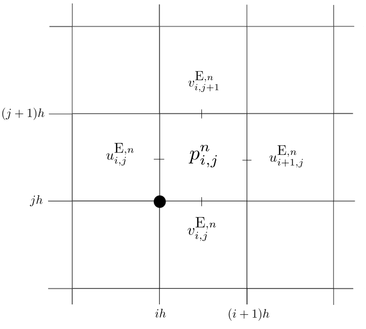
Figure 1: Location of fluid velocity and pressure variables on the staggered marker-and-cell (MAC) grid.

3.3 Spatial Finite Difference Operators

Next, we introduce the discrete difference operators that are used for approximating spatial derivatives. The second derivatives of a scalar Eulerian variable are replaced using the second-order centered difference stencils

$$\mathbbmss{D}_{xx}p_{i,j} =\frac{p_{i+1,j}-2p_{i,j}+p_{i-1,j}}{h^{2}}$$

$$\mbox{and}\qquad\mathbbmss{D}_{yy}p_{i,j} =\frac{p_{i,j+1}-2p_{i,j}+p_{i,j-1}}{h^{2}}.$$

The same operators may be applied to the vector velocity, so that for example

$$\mathbbmss{D}_{xx}\boldsymbol{u}^{\text{E}}_{i,j}=\left[\begin{array}[]{c}\mathbbmss{D}_{xx}u^{\text{E}}_{i,j}\\[5.69046pt] \mathbbmss{D}_{xx}v^{\text{E}}_{i,j}\end{array}\right].$$

Since the fluid pressure and velocity variables are defined at different locations (i.e., cell centers and edges respectively), we also require difference operators whose input and output are at different locations, and for this purpose we indicate explicitly the locations of the input and output using a superscript of the form ${}^{\text{\emph{Input}$\to$\emph{Output}}}$. For example, an operator with the superscript ${}^{\text{C$\to$\text{E}}}$ takes a cell-centered input variable (denoted “C”) and returns an output value located on a cell edge (denoted “E”). Using this notation, we may then define the discrete gradient operator $\mathbbmss{G}^{\text{C}\to\text{E}}$ as

$$\mathbbmss{G}^{\text{C}\to\text{E}}p_{i,j}=\left(\frac{p_{i,j}-p_{i-1,j}}{h},~{}\frac{p_{i,j}-p_{i,j-1}}{h}\right),$$

which acts on the cell-centered pressure variable and returns a vector-valued quantity on the edges of a cell. Likewise, the discrete divergence of the edge-valued velocity

$$\mathbbmss{D}^{\text{E}\to\text{C}}\cdot\boldsymbol{u}_{i,j}^{\text{E}}=\frac{u_{i+1,j}-u_{i,j}}{h}+\frac{v_{i,j+1}-v_{i,j}}{h},$$

which returns a cell-centered value.

Difference formulas are also required for Lagrangian variables such as $\boldsymbol{X}_{k}$, for which we use the first-order one-sided difference approximations:

$$\mathbbmss{D}_{s}^{+}\boldsymbol{X}_{k} =\frac{\boldsymbol{X}_{k+1}-\boldsymbol{X}_{k}}{h_{s}}$$

$$\mbox{and}~{}~{}~{}\mathbbmss{D}_{s}^{-}\boldsymbol{X}_{k} =\frac{\boldsymbol{X}_{k}-\boldsymbol{X}_{k-1}}{h_{s}}.$$

Finally, when discretizing the integrals in (3) and (6), we require a discrete approximation to the Dirac delta function. Here, we make use of the following approximation

$$\delta_{h}(\boldsymbol{x})=\frac{1}{h^{2}}\phi\left(\frac{x}{h}\right)\phi\left(\frac{y}{h}\right)$$

where

$$\phi(r)=\begin{cases}\frac{1}{8}(3-2|r|+\sqrt{1+4|r|-4r^{2}})&\text{if $0\leq|r|<1$},\\ \frac{1}{8}(5-2|r|-\sqrt{-7+12|r|-4r^{2}})&\text{if $1\leq|r|<2$},\\ 0&\text{if $2\leq|r|$}.\end{cases}$$ (12)

Peskin [50] derives this and other regularized delta function kernels by imposing various desirable smoothness and interpolation properties. We have chosen the form of $\delta_{h}$ in equation (12) because numerical simulations have shown that it offers a good balance between accuracy and cost [6, 27, 57], not to mention that it is currently the approximate delta function that is most commonly applied in other IB simulations.

3.4 IB-GM Algorithm

We are now prepared to describe our algorithm for the IB problem based on the fluid solver of Guermond and Minev [29], which we abbreviate “IB-GM”. The fluid is evolved in time in two main stages, both of which reduce to solving one-dimensional tridiagonal linear systems. In the first stage, the diffusion terms in the momentum equations are integrated in time using the directional-splitting technique proposed by Douglas [13]. The nonlinear advection term on the other hand is dealt with explicitly using the second-order Adams-Bashforth extrapolation

$$N^{n+1/2}=\frac{3}{2}\mathbbmss{N}(\boldsymbol{u}^{\text{E},n}_{i,j})-\frac{1}{2}\mathbbmss{N}(\boldsymbol{u}^{\text{E},n-1}_{i,j}),$$ (13)

where $\mathbbmss{N}(\mbox{\raisebox{1.5pt}{\scriptsize$\bullet$}})$ is an approximation of the advection term $\boldsymbol{u}\cdot\nabla\boldsymbol{u}$. In this paper, we write the advection term in skew-symmetric form

$$\mathbbmss{N}(\boldsymbol{u})\approx\frac{1}{2}\boldsymbol{u}\cdot\nabla\boldsymbol{u}+\frac{1}{2}\nabla\cdot(\boldsymbol{u}\boldsymbol{u}),$$ (14)

and then discretize the resulting expression using the second-order centered difference scheme studied by Morinishi et al. [45].

In the second stage, the correction term $\psi$ is calculated using Guermond and Minev’s splitting operator [29], and the actual pressure variable is updated using the higher-order variant of their algorithm corresponding to (9)–(11). For all simulations, we use the same parameter values $\chi=0.6$ and $\epsilon=\Delta t$.

For the remaining force spreading and velocity interpolation steps, we apply standard techniques. The integrals appearing in equations (3) and (6) are approximated to second order using the trapezoidal quadrature rule and the fiber evolution equation (6) is integrated using the second-order Adams-Bashforth extrapolation.

Assuming that the state variables are known at the $(n-1)$th and $n$th time steps, the IB-GM algorithm proceeds as follows.

Step 1.

Evolve the IB position to time $t_{n+1/2}=(n+1/2)\Delta t$:

1. Interpolate the fluid velocity onto immersed boundary points:

   $$\boldsymbol{U}^{n}_{k}=\sum_{i,j}\boldsymbol{u}^{\text{E},n}_{i,j}\delta_{h}(\boldsymbol{x}^{\text{E}}_{i,j}-\boldsymbol{X}^{n}_{k})\,h^{2}.$$

2. Evolve the IB position to time $t_{n+1}$ using an Adams-Bashforth discretization of (6):

   $$\frac{\boldsymbol{X}^{n+1}_{k}-\boldsymbol{X}^{n}_{k}}{\Delta t}=\frac{3}{2}\boldsymbol{U}^{n}_{k}-\frac{1}{2}\boldsymbol{U}^{n-1}_{k}.$$

3. Approximate the IB position at time $t_{n+1/2}$ using the arithmetic average:

   $$\boldsymbol{X}^{n+1/2}_{k}=\frac{1}{2}\left(\boldsymbol{X}^{n+1}_{k}+\boldsymbol{X}^{n}_{k}\right).$$

Step 2.

Calculate the fluid forcing term:

1. Approximate the IB force density at time $t_{n+1/2}$ using (5):

   $$\boldsymbol{F}^{n+1/2}_{k}=\sigma\mathbbmss{D}_{s}^{-}\left(\mathbbmss{D}_{s}^{+}\boldsymbol{X}_{k}^{n+1/2}\left(\mathbbmss{1}-\frac{L}{\left|\mathbbmss{D}_{s}^{+}\boldsymbol{X}_{k}^{n+1/2}\right|}\right)\right).$$

2. Spread the IB force density onto fluid grid points:

   $$\boldsymbol{f}^{\text{E},n+1/2}_{i,j}=\sum_{k}\boldsymbol{F}^{n+1/2}_{k}\,\delta_{h}(\boldsymbol{x}^{\text{E}}_{i,j}-\boldsymbol{X}^{n+1/2}_{k})\,h_{s}.$$

Step 3.

Solve the incompressible Navier–Stokes equations:

1. Predict the fluid pressure at time $t_{n+1/2}$:

   $$p^{\text{\large$\ast$},n+1/2}_{i,j}=p^{n-1/2}_{i,j}+\psi^{n-1/2}_{i,j}.$$

2. Compute the first intermediate velocity field $\boldsymbol{u}^{\text{E},\text{\large$\ast$}}$ by integrating the momentum equations explicitly:

   $$\rho\left(\frac{\boldsymbol{u}^{\text{E},\text{\large$\ast$}}_{i,j}-\boldsymbol{u}^{\text{E},n}_{i,j}}{\Delta t}+{N}^{n+1/2}\right)=\\ \mu\left(\mathbbmss{D}_{xx}+\mathbbmss{D}_{yy}\right)\boldsymbol{u}^{\text{E},n}_{i,j}-\mathbbmss{G}^{\text{C}\to\text{E}}p^{\text{\large$\ast$},n+1/2}_{i,j}+\boldsymbol{f}^{\text{E},n+1/2}_{i,j}.$$

3. Determine the second intermediate velocity $\boldsymbol{u}^{\text{E},\text{\large$\ast$}\text{\large$\ast$}}$ by solving the tridiagonal systems corresponding to the $x$-derivative in the directional-split Laplacian:

   $$\rho\left(\frac{\boldsymbol{u}^{\text{E},\text{\large$\ast$}\text{\large$\ast$}}_{i,j}-\boldsymbol{u}^{\text{E},\text{\large$\ast$}}_{i,j}}{\Delta t}\right)=\frac{\mu}{2}\mathbbmss{D}_{xx}\left(\boldsymbol{u}^{\text{E},\text{\large$\ast$}\text{\large$\ast$}}_{i,j}-\boldsymbol{u}^{\text{E},n}_{i,j}\right).$$

4. Obtain the final velocity approximation at time $t_{n+1}$ by solving the following tridiagonal systems corresponding to the $y$-derivative piece of the directional-split Laplacian for $\boldsymbol{u}^{\text{E},n+1}_{i,j}$:

   $$\rho\left(\frac{\boldsymbol{u}^{\text{E},n+1}_{i,j}-\boldsymbol{u}^{\text{E},\text{\large$\ast$}\text{\large$\ast$}}_{i,j}}{\Delta t}\right)=\frac{\mu}{2}\mathbbmss{D}_{yy}\left(\boldsymbol{u}^{\text{E},n+1}_{i,j}-\boldsymbol{u}^{\text{E},n}_{i,j}\right).$$

5. Determine the pressure correction term $\psi_{i,j}^{n+1/2}$ by solving

   $$\left(\mathbbmss{1}-\mathbbmss{D}_{xx}\right)\left(\mathbbmss{1}-\mathbbmss{D}_{yy}\right)\psi_{i,j}^{n+1/2}=-\frac{\rho}{\Delta t}\mathbbmss{D}^{\text{E}\to\text{C}}\cdot\boldsymbol{u}^{\text{E},n+1}_{i,j}.$$

6. Calculate the pressure at time $t_{n+1/2}$ using

   $$p^{n+1/2}_{i,j}=p^{n-1/2}_{i,j}+\psi^{n+1/2}_{i,j}-\chi\mu\mathbbmss{D}^{\text{E}\to\text{C}}\cdot\left(\frac{1}{2}(\boldsymbol{u}^{\text{E},n+1}_{i,j}+\boldsymbol{u}^{\text{E},n}_{i,j})\right).$$

Note that in the first step of the algorithm with $n=0$, we do not yet have an approximation of the solution at the previous time step, and therefore we make the following replacements:

• In Step 1b, approximate the fiber evolution equation using a first-order forward Euler approximation $\boldsymbol{X}^{1}_{k}=\boldsymbol{X}^{0}_{k}+\Delta t\boldsymbol{U}^{0}_{k}$.

• In Step 3a, set $p^{\text{\large$\ast$},1/2}_{i,j}=0$.

• In Step 3b, the nonlinear term from equation (13) is replaced with $N^{1/2}=\mathbbmss{N}(\boldsymbol{u}^{\text{E},0}_{i,j})$.

4 Parallel Implementation

Here we outline the details of the algorithm that relate specifically to the parallel implementation. Since a primary feature of our algorithm is its parallel scaling properties, it is important to discuss our implementation in order to understand the parallel characteristics of the method.

4.1 Partitioning of the Eulerian and Lagrangian Grids

Suppose that the algorithm in section 3.4 is implemented on a distributed-memory computing machine with $P=P_{x}\cdot P_{y}$ processing nodes. The parallelization is performed by subdividing the rectangular domain $\Omega$ into equally-sized rectangular partitions $\{\Omega_{\ell,m}\}$, with $\ell=1,2,\ldots,P_{x}$ and $m=1,2,\ldots,P_{y}$, where $P_{x}$ and $P_{y}$ refer to the number of subdivisions in the $x$– and $y$–directions respectively. Each node is allocated a single domain partition $\Omega_{\ell,m}$, along with the values of the Eulerian and Lagrangian variables contained within it. For example, the $(\ell,m)$ node would contain in its memory the fluid variables $\boldsymbol{u}_{i,j}^{\text{E}}$ and $p_{i,j}$ for all $\boldsymbol{x}_{i,j}\in\Omega_{\ell,m}$, along with all immersed boundary data $\boldsymbol{X}_{k}$ and $\boldsymbol{F}_{k}$ such that $\boldsymbol{X}_{k}\in\Omega_{\ell,m}$. This partitioning is illustrated for a simple $3\times 3$ subdivision in Figure 22.

Figure 2: 2 Parallel domain decomposition with $P_{x}=P_{y}=3$. 2 Communication required to update ghost cell regions for the subdomain $\Omega_{2,2}$.

In this way, the computational work required in each time step is effectively divided between processing nodes by requiring that each node update only those state variables located within its assigned subdomain. This approach is similar to that taken by Uhlmann [62] and Griffith [25], who partitioned the Lagrangian data so that IB points belong to the same processor as the surrounding fluid. An alternate approach would be to independently partition the Eulerian and Lagrangian data as done by Givelberg [19].

The primary novelty in our algorithm derives from that way that it introduces parallelism naturally into the discretization. This differentiates our method from prior approaches (in Griffith [27] or Givelberg [19]) that rely heavily on black-box parallel solvers such as Hypre [15]. In particular, we use a fractional-step scheme that permits the immersed boundary and fluid to be treated independently. The IB component of the algorithm is discretized in the same manner as Griffith [23] who used an Adams-Bashforth discretization to reduce the number of floating-point operations. Since this is an explicit discretization, the discrete immersed boundary can be viewed as a simple particle system – a collection of IB material points connected by force-generating connections – which is a well-established class of problems in the parallel computing community [2, 3]. Therefore, the major differences in parallel implementation come from the discrete delta function whose support allows particles to interact over multiple subdomains in the velocity interpolation and force spreading steps.

For the fluid portion of the algorithm, we use the GM fluid solver as described in [29] with the following minor modifications:

• the advection term is discretized in skew-symmetric form;

• periodic boundary conditions are imposed on the fluid domain;

• the directional-splitting order is rotated in each time step to reduce the possibility of a directional bias; and

• minor alterations are required to the parallel tridiagonal solver.

By using the directional split strategy of Guermond and Minev, the discretized fluid equations deflate into a sequence of one-dimensional problems, which is where parallelism is introduced directly into the discretization. The most significant departure from other common IB schemes is that the GM solver is a pseudo-compressibility method that only approximately satisfies the incompressibility constraint. It is yet to be seen how such a fluid solver will handle the near-singular body forces that occur naturally in IB problems. Therefore, a comprehensive numerical study is required to test the accuracy, convergence, and volume conservation of the method.

Next, we describe our approach for implementing data partitioning and communication, which makes use of infrastructure provided by MPI [17] and PETSc [5]. Since the fluid and immersed boundary are discretized on two separate grids, the data partitioning between nodes must be handled differently in each case. The partitioning of Eulerian variables is much simpler because the spatial locations are fixed in time and remain associated with the same node for the entire computation. In contrast, Lagrangian variables are free to move throughout the fluid domain and so a given IB point may move between two adjacent subdomains during the course of a single time step. As a result, the data structure and communication patterns for the Lagrangian variables are more complex.

Consider the communication required for the update of fluid variables in each time step, for which the algorithm in section 3.4 requires the explicit computation of several discrete difference operators. For points located inside a subdomain $\Omega_{\ell,m}$, the discrete operators are easily computed; however for points on the edge of a domain partition, a difference operator may require data that is not contained in the current node’s local memory. For example, when calculating the discrete Laplacian (using the 5-point stencil), data at points adjacent to the given state variable are required. As a result, when an adjacent variable does not reside in $\Omega_{\ell,m}$, communication is required with a neighbouring node to obtain the required value. This communication is aggregated together using ghost cells that lie inside a strip surrounding each $\Omega_{\ell,m}$ as illustrated in Figure 22. The width of the ghost region is set equal to the support of the discrete delta function used in the velocity interpolation and force spreading steps; that is, two grid points in the case of the delta-approximation (12). When a difference operator is applied to a state variable stored in the $(\ell,m)$ node, the neighbouring nodes communicate the data contained in the ghost cells adjacent to $\Omega_{\ell,m}$. After the ghost region is filled, the discrete difference operators may then be calculated for all points in $\Omega_{\ell,m}$. When combined with the parallel linear solver discussed later in section 4.2, this parallel communication technique permits the fluid variables to be evolved in time.

As the IB points move through the fluid, the number of IB points residing in any particular subdomain can vary from one time step to the next. Therefore, the memory required to store the local IB data structure changes with time, as does the communication load. These complications are dealt with by splitting the data structure defining the immersed boundary into two separate components corresponding to IB points and force connections. The IB point (IB) data structure contains the position and velocity of all IB points resident in a given subdomain, whereas the force connection (FC) data structure keeps track of all force-generating connections between these points. The force density calculations depend on spatial information and so the IB data structure requires a globally unique index (which we call the “primary key”) that is referenced by the FC data structure (the “foreign key”). This relationship is illustrated in Figure 3, where the force connections shown are consistent with the elastic force function (5). If the IB data structure is represented as an associative array using PointID as the key (and referenced as IB[PointID]) and FC[i] represents a specific element of the force connection array, then the force density calculation may be written as

$$\texttt{FC[i].Fdens}=\frac{\texttt{FC[i].sigma}}{h_{s}^{2}}\,\big{(}\,\texttt{IB[\,FC[i].LPointID\,].X}\;+\;\texttt{IB[\,FC[i].RPointID\,].X}\\ -\;\texttt{2 * IB[\,FC[i].PointID\,].X}\,\big{)},$$

where we have assumed here that the force parameter $L=0$. The IB and FC data structures are stored in a hash table and vector (respectively) using the standard STL containers in C++.

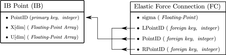
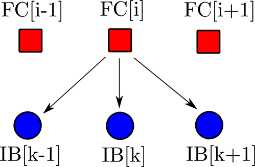
Figure 3: 3 Relationship between the data structures for the IB points (IB) and elastic force connections (FC). 3 References from a chosen force connection to the corresponding IB points.

We are now prepared to summarize the complete parallel procedure that is used to evolve the fluid and immersed boundary. Keep in mind that at the beginning of each time step, a processing node contains only those IB points and force connections that reside in the corresponding subdomain. The individual solution steps are:

• Velocity interpolation: Interpolate the fluid velocity onto the IB points and store the result in IB[$\bullet$].U. This step requires fluid velocity data from the ghost region.

• Immersed boundary evolution: Evolve the IB points in time by updating $\texttt{IB[\mbox{\raisebox{1.5pt}{\scriptsize$\bullet$}}].X}=\boldsymbol{X}^{n+1}_{\mbox{\raisebox{1.5pt}{\scriptsize$\bullet$}}}$. Note that the IB point position at the half time step ($\texttt{IB[\mbox{\raisebox{1.5pt}{\scriptsize$\bullet$}}].Xh}=\boldsymbol{X}^{n+1/2}_{\mbox{\raisebox{1.5pt}{\scriptsize$\bullet$}}}$) must also be stored for the force spreading step.

• Immersed boundary communication: Send the data from IB points lying within the ghost region to the neighbouring processing nodes. Figure 4 illustrates how the IB points residing in the ghost region corresponding to $\Omega_{\ell,m}$ are copied from $\Omega_{\ell+1,m}$ (for both the full time step $n+1$ and the half-step $n+1/2$). In this example, three IB points (corresponding to $\texttt{PointID}=k,k+1,k+2$) and two force connections (with $\texttt{FC[i].PointID}=k,k+1$) are communicated to $\Omega_{\ell,m}$. The additional IB point is required to calculate the force density for $\texttt{FC[i].PointID}=k+1$. Because the IB point $k-1$ already resides in $\Omega_{\ell,m}$, the force density can be computed for $\texttt{FC[i].PointID}=k$ without any additional communication.

• Force spreading: Calculate the force density for all IB points in $\Omega_{\ell,m}$ and the surrounding ghost region at the time step $n+1/2$. Then spread the force density onto the Eulerian grid points residing in $\Omega_{\ell,m}$.

• Immersed boundary cleanup: Remove all IB points and corresponding force connections that do not reside in $\Omega_{\ell,m}$ at time step $n+1$.

• Evolve fluid: Evolve the fluid variables in time using the parallel techniques discussed above. This requires communication with the neighbouring processing nodes to update the ghost cell region, and further communication is needed while solving the linear systems.

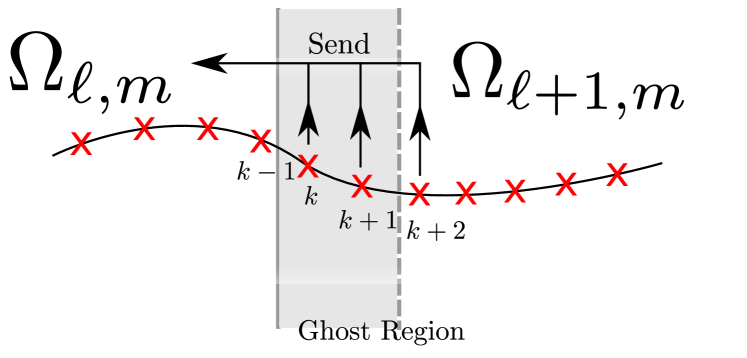
Figure 4: IB points inside the ghost region surrounding $\Omega_{\ell,m}$ are communicated from $\Omega_{\ell+1,m}$.

Using the approach outlined above, each processing node only needs to communicate with its neighbouring nodes, with the only exception being the linear solver which we address in the next section. Since communication often hinders the performance of a parallel algorithm, this is the property that allows our method to scale so well. For example, if the problem size and number of processing nodes are doubled, then we would ideally want the execution time per time step to remain unchanged.

4.2 Linear Solver

A key remaining component of the algorithm outlined in section 3.4 is the solution of the tridiagonal linear systems arising in the fluid solver. When solving the momentum equations the following linear systems arise:

$$\left(\mathbbmss{1}-\frac{\mu\Delta t}{2\rho}\mathbbmss{D}_{xx}\right)\boldsymbol{u}^{\text{E},\text{\large$\ast$}\text{\large$\ast$}}_{i,j}=\boldsymbol{u}^{\text{E},\text{\large$\ast$}}_{i,j}-\frac{\mu\Delta t}{2\rho}\mathbbmss{D}_{xx}\boldsymbol{u}^{\text{E},n}_{i,j},$$ (15)

$$\left(\mathbbmss{1}-\frac{\mu\Delta t}{2\rho}\mathbbmss{D}_{yy}\right)\boldsymbol{u}^{\text{E},n+1}_{i,j}=\boldsymbol{u}^{\text{E},\text{\large$\ast$}\text{\large$\ast$}}_{i,j}-\frac{\mu\Delta t}{2\rho}\mathbbmss{D}_{yy}\boldsymbol{u}^{\text{E},n}_{i,j},$$ (16)

while the pressure update step requires solving

$$\left(\mathbbmss{1}-\mathbbmss{D}_{xx}\right)\left(\mathbbmss{1}-\mathbbmss{D}_{yy}\right)\psi_{i,j}^{n+1/2}=-\frac{\rho}{\Delta t}\mathbbmss{D}^{\text{E}\to\text{C}}\cdot\boldsymbol{u}^{\text{E},n+1}_{i,j}.$$

This last equation can be split into two steps

$$\left(\mathbbmss{1}-\mathbbmss{D}_{xx}\right)\psi_{i,j}^{\text{\large$\ast$},n+1/2} =-\frac{\rho}{\Delta t}\mathbbmss{D}^{\text{E}\to\text{C}}\cdot\boldsymbol{u}^{\text{E},n+1}_{i,j},$$ (17)

$$\mbox{and}\qquad\left(\mathbbmss{1}-\mathbbmss{D}_{yy}\right)\psi_{i,j}^{n+1/2} =\psi_{i,j}^{\text{\large$\ast$},n+1/2},$$ (18)

where $\psi_{i,j}^{\text{\large$\ast$}}$ is an intermediate variable. Note that each linear system in (15)–(18) involves a difference operator that acts in one spatial dimension only and decouples into a set of one-dimensional periodic (or cyclic) tridiagonal systems. For example, equations (15) and (17) consist of $N$ tridiagonal systems of size $N\times N$ having the general form

$$\mathbbmss{A}^{(j)}\Psi_{i,j}=b_{i,j},$$ (19)

for each $j=0,1,\ldots,N-1$.

Because the processing node $(\ell,m)$ contains only fluid data residing in subdomain $\Omega_{\ell,m}$, these tridiagonal linear systems divide naturally between nodes. Each node solves those linear systems for which it has the corresponding data $b_{i,j}\in\Omega_{\ell,m}$ as illustrated in Figure 5. For example, when solving (19) along the $x$-direction, each processing node solves $N/P_{y}$ linear systems and the total work is spread over $P_{x}$ nodes. Similarly, when solving the corresponding systems along the $y$-direction, each processing node solves $N/P_{x}$ systems spread over $P_{y}$ nodes.

Figure 5: 5 Coupling direction for linear systems (15) and (18). 5 Coupling direction for linear systems (16) and (17). Each processing node participates in solving $N/P_{x,y}$ tridiagonal systems and requires communication in the direction of the arrows.

Each periodic tridiagonal system is solved directly using a Schur-complement technique [54, sec. 14.2.1]. This is achieved by rewriting the linear equations as a block-structured system where the interfaces between blocks correspond to those for the subdomains. To illustrate, let us consider an example with $P=2$ processors only, for which the periodic tridiagonal system

$$\left[\begin{array}[]{cccccccccc}a_{1}&b_{1}&&&&&&&&c_{1}\\ c_{2}&a_{2}&b_{2}&&&&&&&\\ &&\ddots&&&&&&&\\ &&&\ddots&&&&&&\\ &&&c_{M-1}&a_{M-1}&b_{M-1}&&&&\\ \hline\cr&&&&c_{M}&a_{M}&b_{M}&&&\\ &&&&&c_{M+1}&a_{M+1}&b_{M+1}&&\\ &&&&&&&\ddots&&\\ &&&&&&&&\ddots&\\ b_{N}&&&&&&&&c_{N}&a_{N}\end{array}\right]\left[\begin{array}[]{c}y_{1}\\ x_{2}\\ \vdots\\ \vdots\\ x_{M-1}\\ \hline\cr y_{2}\\ x_{M+1}\\ \vdots\\ \vdots\\ x_{N}\end{array}\right]=\left[\begin{array}[]{c}g_{1}\\ f_{2}\\ \vdots\\ \vdots\\ f_{M-1}\\ \hline\cr g_{2}\\ f_{M+1}\\ \vdots\\ \vdots\\ f_{N}\end{array}\right]$$

arises from a single row of unknowns in Figure 55 (or a single column in Figure 55). In this example, the indices $M-1$ and $M$ refer to the subdomain boundary points (denoted with a vertical line in the matrix above) so that the data ($y_{1}$, $x_{2}$, …, $x_{M-1}$, $g_{1}$, $f_{2}$, …, $f_{M-1}$) reside on processor 1 and ($y_{2}$, $x_{M+1}$, …, $x_{N}$, $g_{2}$, $f_{M+1}$, …, $f_{N}$) on processor 2. To isolate the coupling between subdomains, the rows in the matrix are reordered to shift the unknowns at periodic subdomain boundaries ($y_{1}$ and $y_{2}$) to the last two rows, and then the columns are reordered to keep the diagonal entries on the main diagonal. This yields the equivalent linear system

$$\left[\begin{array}[]{cccc!{\colorvline}cccc!{\colorvline}cc}a_{2}&b_{2}&&\hfil\lx@intercol\color[rgb]{.75,.75,.75}\vrule&&&&\hfil\lx@intercol\color[rgb]{.75,.75,.75}\vrule&c_{2}&\\ &\ddots&&\hfil\lx@intercol\color[rgb]{.75,.75,.75}\vrule&&&&\hfil\lx@intercol\color[rgb]{.75,.75,.75}\vrule&&\\ &&\ddots&\hfil\lx@intercol\color[rgb]{.75,.75,.75}\vrule&&&&\hfil\lx@intercol\color[rgb]{.75,.75,.75}\vrule&&\\ &&c_{M-1}&a_{M-1}\hfil\lx@intercol\color[rgb]{.75,.75,.75}\vrule&&&&\hfil\lx@intercol\color[rgb]{.75,.75,.75}\vrule&&b_{M-1}\\ \hline\cr&&&\hfil\lx@intercol\color[rgb]{.75,.75,.75}\vrule&a_{M+1}&b_{M+1}&&\hfil\lx@intercol\color[rgb]{.75,.75,.75}\vrule&&c_{M+1}\\ &&&\hfil\lx@intercol\color[rgb]{.75,.75,.75}\vrule&&\ddots&&\hfil\lx@intercol\color[rgb]{.75,.75,.75}\vrule&&\\ &&&\hfil\lx@intercol\color[rgb]{.75,.75,.75}\vrule&&&\ddots&\hfil\lx@intercol\color[rgb]{.75,.75,.75}\vrule&&\\ &&&\hfil\lx@intercol\color[rgb]{.75,.75,.75}\vrule&&&c_{N}&a_{N}\hfil\lx@intercol\color[rgb]{.75,.75,.75}\vrule&b_{N}&\\ \hline\cr b_{1}&&&\hfil\lx@intercol\color[rgb]{.75,.75,.75}\vrule&&&&c_{1}\hfil\lx@intercol\color[rgb]{.75,.75,.75}\vrule&a_{1}&\\ &&&c_{M}\hfil\lx@intercol\color[rgb]{.75,.75,.75}\vrule&b_{M}&&&\hfil\lx@intercol\color[rgb]{.75,.75,.75}\vrule&&a_{M}\end{array}\right]\left[\begin{array}[]{c}x_{2}\\ \vdots\\ \vdots\\ x_{M-1}\\ \hline\cr x_{M+1}\\ \vdots\\ \vdots\\ x_{N}\\ \hline\cr y_{1}\\ y_{2}\end{array}\right]=\left[\begin{array}[]{c}f_{2}\\ \vdots\\ \vdots\\ f_{M-1}\\ \hline\cr f_{M+1}\\ \vdots\\ \vdots\\ f_{N}\\ \hline\cr g_{1}\\ g_{2}\end{array}\right],$$

which has the block structure

$$\left[\begin{array}[]{ccc}\boldsymbol{B}_{1}&&\boldsymbol{E}_{1}\\ &\boldsymbol{B}_{2}&\boldsymbol{E}_{2}\\ \boldsymbol{F}_{1}&\boldsymbol{F}_{2}&\boldsymbol{C}\end{array}\right]\left[\begin{array}[]{c}\boldsymbol{x}_{1}\\ \boldsymbol{x}_{2}\\ \boldsymbol{y}\end{array}\right]=\left[\begin{array}[]{c}\boldsymbol{f}_{1}\\ \boldsymbol{f}_{2}\\ \boldsymbol{g}\end{array}\right].$$

In the more general situation with $P$ subdomains, the block structure becomes

$$\left[\begin{array}[]{ccccc}\boldsymbol{B}_{1}&&&&\boldsymbol{E}_{1}\\ &\boldsymbol{B}_{2}&&&\boldsymbol{E}_{2}\\ &&\ddots&&\vdots\\ &&&\boldsymbol{B}_{P}&\boldsymbol{E}_{P}\\ \boldsymbol{F}_{1}&\boldsymbol{F}_{2}&\cdots&\boldsymbol{F}_{P}&\boldsymbol{C}\end{array}\right]\left[\begin{array}[]{c}\boldsymbol{x}_{1}\\ \boldsymbol{x}_{2}\\ \vdots\\ \boldsymbol{x}_{P}\\ \boldsymbol{y}\end{array}\right]=\left[\begin{array}[]{c}\boldsymbol{f}_{1}\\ \boldsymbol{f}_{2}\\ \vdots\\ \boldsymbol{f}_{P}\\ \boldsymbol{g}\end{array}\right],$$

or more compactly

$$\left[\begin{array}[]{ccc}\boldsymbol{B}&\boldsymbol{E}\\ \boldsymbol{F}&\boldsymbol{C}\\ \end{array}\right]\left[\begin{array}[]{c}\boldsymbol{x}\\ \boldsymbol{y}\end{array}\right]=\left[\begin{array}[]{c}\boldsymbol{f}\\ \boldsymbol{g}\end{array}\right],$$ (26)

where $\boldsymbol{C}\in\mathbb{R}^{P\times P}$, $\boldsymbol{B}\in\mathbb{R}^{(N-P)\times(N-P)}$, $\boldsymbol{E}\in\mathbb{R}^{(N-P)\times P}$, and $\boldsymbol{F}\in\mathbb{R}^{P\times(N-P)}$. Here, $\boldsymbol{x}$ and $\boldsymbol{f}$ denote the data located in the interior of a subdomain while $\boldsymbol{y}$ and $\boldsymbol{g}$ denote the data residing on the interface between subdomains. Next, we use the LU factorization to rewrite the block matrix from (26) as

$$\left[\begin{array}[]{ccc}\boldsymbol{B}&\boldsymbol{E}\\ \boldsymbol{F}&\boldsymbol{C}\\ \end{array}\right]=\left[\begin{array}[]{ccc}\boldsymbol{I}&\boldsymbol{0}\\ \boldsymbol{F}\boldsymbol{B}^{-1}&\boldsymbol{I}\end{array}\right]\left[\begin{array}[]{ccc}\boldsymbol{B}&\boldsymbol{E}\\ \boldsymbol{0}&\boldsymbol{S}\end{array}\right],$$

where $\boldsymbol{S}=\boldsymbol{C}-\boldsymbol{F}\boldsymbol{B}^{-1}\boldsymbol{E}$ is the Schur complement. Using this factorized form, we can decompose the block system into the following three smaller problems:

$$\boldsymbol{B}\boldsymbol{f}^{\text{\large$\ast$}} =\boldsymbol{f},$$ (27)

$$\boldsymbol{S}\boldsymbol{y} =\boldsymbol{g}-\boldsymbol{F}\boldsymbol{f}^{\text{\large$\ast$}},$$ (28)

$$\boldsymbol{B}\boldsymbol{x} =\boldsymbol{B}\boldsymbol{f}^{\text{\large$\ast$}}-\boldsymbol{E}\boldsymbol{y}.$$ (29)

Based on this decomposition, we can now summarize the solution procedure as follows:

• Local tridiagonal solver: Each processor solves a local non-periodic tridiagonal system

  $$\boldsymbol{B}_{p}\boldsymbol{f}^{\text{\large$\ast$}}_{p}=\boldsymbol{f}_{p},$$

  which can be solved efficiently using Thomas’s algorithm. The matrices $\boldsymbol{B}_{p}$ are the non-periodic tridiagonal blocks in the block diagonal matrix $\boldsymbol{B}$.

• Gather data to master node: Each processor sends three scalar values to the master node corresponding to the first and last entries of the vector $\boldsymbol{f}^{\text{\large$\ast$}}_{p}$, as well as the scalar $g_{p}$. Because $\boldsymbol{F}_{p}$ is sparse, only a few values are required to construct the right hand side of the Schur complement system.

• Solve Schur complement system: On the master node, solve the reduced $P\times P$ Schur complement system (28). Based on the sparsity patterns of $\boldsymbol{F}$ and $\boldsymbol{E}$, the Schur complement matrix $\boldsymbol{S}$ is periodic and tridiagonal and therefore can be inverted efficiently using Thomas’s algorithm.

• Scatter data from master node: The master node scatters two scalar values from $\boldsymbol{y}$ to each processor. Because of the sparsity of $\boldsymbol{B}^{-1}\boldsymbol{E}$, only a few values of $\boldsymbol{y}$ are required in the next step. Therefore, the $p$th processor only requires the entries of $\boldsymbol{y}$ numbered $p$ and $\text{mod}(p+1,P)$.

• Correct local solution: Each processor corrects its local solution

  $$\boldsymbol{x}_{p}=\boldsymbol{f}^{\text{\large$\ast$}}_{p}-\boldsymbol{B}^{-1}_{p}\boldsymbol{E}_{p}\boldsymbol{y},$$

  using the local values $\boldsymbol{f}^{\text{\large$\ast$}}_{p}$ computed in the first step.

The tridiagonal systems above can be parallelized very efficiently. As already indicated earlier, this procedure only requires two collective communications – scatter and gather – and because global communication only occurs along one spatial direction the communication overhead increases only marginally with the number of processors. A further cost savings derives from the fact that the tridiagonal systems do not change from one time step to the next, and so the matrices $\boldsymbol{S}$ and $\boldsymbol{B}^{-1}\boldsymbol{E}$ can be precomputed.

The only potential bottleneck in this procedure is in solving the reduced Schur complement system (28). Since the reduced system is solved only on the master node, clock cycles on the remaining idle nodes are wasted at this time. Furthermore, this wasted time increases as the number of processors increase since the Schur complement system grows with $P$. Fortunately, the IB algorithm never solves just a single tridiagonal system. For example, when solving (19) in the $x$-direction, $P=P_{x}$ processing nodes work together to solve $N/P_{y}$ tridiagonal systems. Therefore, the $N/P_{y}$ systems when solved together require solving $N/P_{y}$ different Schur complement systems. This workload can be spread out evenly between the $P$ processors thereby keeping all processors occupied.

5 Numerical Results

To test the accuracy of our algorithm, we consider two model problems. The first is an idealized one-dimensional elliptical membrane with zero thickness that is immersed in a 2D fluid and undergoes a damped periodic motion. Here, the immersed boundary exerts a singular force on the fluid and results in a pressure jump across the membrane that reduces the method’s order of accuracy. The second model problem is a generalization of the first in which we consider a thick immersed boundary, made up of multiple fiber layers in which the elastic stiffness is reduced smoothly to a value of zero at the edges. By providing the immersed boundary in this example with a physical thickness, the external force is no longer singular, which then leads to higher-order convergence rates.

5.1 Thin Ellipse

For our first 2D model problem, the initial configuration is an elliptical membrane with semi-axes $r_{1}$ and $r_{2}$, parameterized by

$$\boldsymbol{X}(s,0)=\left(\frac{1}{2}+r_{1}\cos(2\pi s),~{}\frac{1}{2}+r_{2}\sin(2\pi s)\right),$$

with $s\in[0,1]$. The ellipse is placed in a unit square containing fluid that is initially stationary with $\boldsymbol{u}(\boldsymbol{x},0)=0$. We see from the solution snapshots in Figure 6 that the elastic membrane undergoes a damped periodic motion, oscillating back and forth between elliptical shapes having a semi-major axis aligned with the $x$- and $y$-directions. The amplitude of the oscillations decreases over time, and the membrane tends ultimately toward a circular equilibrium state with radius approximately equal to $\sqrt{r_{1}r_{2}}$ (which has the same area as the initial ellipse).

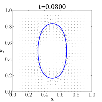
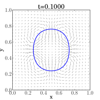
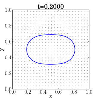
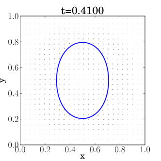
Figure 6: Snapshots of a thin oscillating ellipse using the GM-IB method, with parameters $\sigma=1$, $N=256$ and $\Delta t=0.04/512$.

For this problem, we actually computed results using two immersed boundary algorithms corresponding to different fluid solvers. The first algorithm, denoted GM-IB, is the same one described in section 3.4 that uses Guermond and Minev’s fluid solver. The second algorithm, denoted BCM-IB, is identical to the first except that the fluid solver is replaced with the second-order projection method described by Brown, Cortez, and Minion [7]. We take values of the parameters from Griffith [23], who used $\mu=0.01$, $\rho=1$, $r_{1}=\frac{5}{28}$, $r_{2}=\frac{7}{20}$ and $N_{s}=\frac{19}{4}N$. We then compare our numerical results for different choices of the membrane elastic stiffness ($\sigma$) and spatial discretization ($N$). Unless stated otherwise, the time step is chosen so that the simulation is stable on the finest spatial grid (with $N=512$). This is a conservative choice for the time step that attempts to avoid any unreasonable accumulation of errors in time, but it also provides limited information regarding the time step restrictions for the two methods. However, we observe in practice that there is little difference between the time step restrictions for the GM-IB and BCM-IB algorithms, although GM-IB does have a slightly stricter time step restriction than BCM-IB.

Because the fluid contained within the immersed boundary cannot escape, the area of the oscillating ellipse should remain constant in time. However, many other IB computations for this thin ellipse problem exhibit poor volume conservation which manifests itself as an apparent “leakage” of fluid out of the immersed boundary. The source of this volume conservation error is numerical error in the discrete divergence-free condition for the interpolated velocity field located on immersed boundary points, which can be non-zero even when the fluid solver guarantees that the velocity is discretely divergence-free on the Eulerian fluid grid [46, 51]. Griffith [23] observed that volume conservation can be improved by using a pressure-increment fluid solver instead of a pressure-free solver, and furthermore that fluid solvers based on a staggered grid tended to perform better than those using a collocated grid. We have employed both of these ideas in our proposed method and so we expect to see significant improvement in volume conservation relative to other IB methods.

We begin by plotting the maximum and mean radii of the ellipse versus time in Figure 77, from which it is clear that the immersed boundary converges to a circular steady state having radius $\sqrt{r_{1}r_{2}}=\frac{1}{4}$. The BCM-IB results are indistinguishable from those using GM-IB, and so only the latter are depicted in this figure. The low rate of volume loss observed in both algorithms is consistent with the numerical experiments of Griffith [23]. Owing to the relatively high Reynolds number for this flow ($\mbox{Re}\approx 150$) there exists a noticeable error in the oscillation frequency for coarser discretizations, although we note that this error is much smaller for lower Re flows. We suspect that this frequency error could be reduced significantly by employing higher-order approximations in the nonlinear advection term and the IB evolution equation (6), such as has been done by Griffith [24]. Finally, we note that Figure 77 shows that the GM-IB algorithm captures the discontinuity in pressure without any visible oscillations.

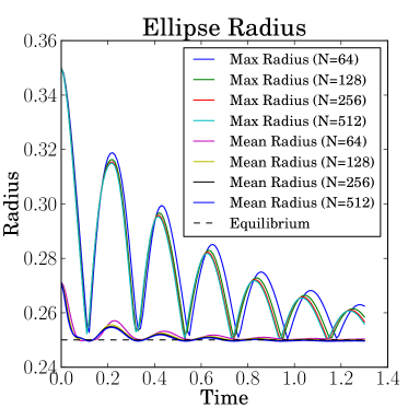
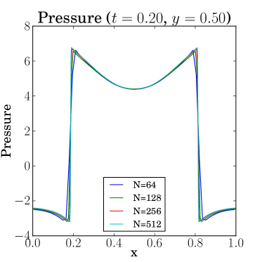
Figure 7: Results for the thin ellipse problem using the GM-IB method with $\sigma=1$ and $\Delta t=0.04/512$. 7 Maximum and mean radii. 7 Pressure slices across the $x$–axis with $y=0.5$ and $t=0.2$.

We next estimate the error and convergence rate for both algorithms. Because the thin ellipse problem is characterized by a singular IB force, there is a discontinuity in velocity derivatives and pressure and so our numerical scheme is limited to first order accuracy. We note that improvements in the convergence rate could be achieved by explicitly incorporating these discontinuities into the difference scheme, for example as is done in the immersed interface method [38, 39].

When reporting the error in a discrete variable $q_{N}$ that is approximated on a grid at refinement level $N$, we use the notation

$${\mathcal{E}}\left[q;N\right]=\|q_{N}-q_{\text{exact}}\|_{2}.$$ (30)

Because the exact solution for the thin ellipse problem is not known, we estimate $q_{\text{exact}}$ by using the approximate solution on the finest mesh corresponding to $N_{f}=512$ with the BCM-IB algorithm, and then take $q_{\text{exact}}=\mathcal{I}^{N_{f}\to N}q_{N_{f}}$, where $\mathcal{I}^{N_{f}\to N}$ is an operator that interpolates the finest mesh solution $q_{N_{f}}$ onto the current coarse mesh with $N$ points. We use the discrete $\ell^{2}$ norm to estimate errors, which is calculated for an Eulerian quantity such as the pressure using

$$\|p_{i,j}\|_{2}=\left(h^{2}\sum_{i,j}|p_{i,j}|^{2}\right)^{1/2},$$ (31)

and similarly for a Lagrangian quantity such as the IB position using

$$\|\boldsymbol{X}_{k}\|_{2}=\left(h_{s}\sum_{k}|\boldsymbol{X}_{k}|^{2}\right)^{1/2},$$ (32)

where $|\cdot|$ represents the absolute value in the first formula and the Euclidean distance in the second. The convergence rate can then be estimated using solutions $q_{N}$, $q_{2N}$ and $q_{4N}$ on successively finer grids as

$${\mathcal{R}}\left[q;N\right]=\log_{2}\left(\frac{\|q_{N}-\mathcal{I}^{2N\to N}q_{2N}\|_{2}}{\|q_{2N}-\mathcal{I}^{4N\to 2N}q_{4N}\|_{2}}\right).$$ (33)

A summary of convergence rates and errors is given in Tables 1 and 2 for both the GM-IB and BCM-IB algorithms, taking different values of the elastic stiffness parameter $\sigma$. The error in all cases is measured at a time three-quarters through the ellipse’s first oscillation, when the membrane is roughly circular in shape. Table 1 clearly shows that the two algorithms exhibit similar convergence rates for all state variables. First-order convergence is seen in both the fluid velocity and membrane position, while the pressure shows the expected reduction in accuracy to ${\mathcal{O}}\left(h^{1/2}\right)$ owing to the pressure discontinuity. The errors in Table 2 show that GM-IB and BCM-IB are virtually indistinguishable from each other except for the error in the divergence-free condition, ${\mathcal{E}}\left[\nabla\cdot\boldsymbol{u};N\right]$, where the BCM-IB algorithm appears to enforce the incompressibility constraint better than GM-IB. Because Guermond and Minev’s fluid solver does not project the velocity field onto the space of divergence-free velocity fields (even approximately), it is not surprising that BCM-IB performs better in this regard. We remark that the magnitude of the fluid variables increases with the stiffness $\sigma$, so that the error increases as well (since ${\cal E}$ is defined as an absolute error measure); however, the relative error and convergence rates remain comparable as $\sigma$ varies over several orders of magnitude.

Table 1: Estimated $\ell^{2}$ convergence rates for the thin ellipse problem with three different parameter sets: ($\sigma=0.1$, $t=1.06$, $\Delta t=0.08/512$), ($\sigma=1$, $t=0.31$, $\Delta t=0.04/512$), ($\sigma=10$, $t=0.0975$, $\Delta t=0.01/512$).

		${\mathcal{R}}\left[\boldsymbol{u};N\right]$		${\mathcal{R}}\left[p;N\right]$		${\mathcal{R}}\left[\boldsymbol{X};N\right]$
$\sigma$	$N$	GM	BCM	GM	BCM	GM	BCM
$0.1$	$64$	$1.02$	$1.02$	$0.55$	$0.55$	$1.46$	$1.46$
	$128$	$1.05$	$1.06$	$0.53$	$0.53$	$1.28$	$1.29$
$1$	$64$	$1.48$	$1.51$	$0.72$	$0.73$	$1.34$	$1.35$
	$128$	$0.96$	$1.03$	$0.57$	$0.58$	$1.31$	$1.37$
$10$	$64$	$1.27$	$1.33$	$0.88$	$0.84$	$1.35$	$1.33$
	$128$	$0.89$	$1.03$	$0.68$	$0.82$	$1.32$	$1.71$

Table 2: Estimated $\ell^{2}$ errors the thin ellipse problem with three different parameter sets: ($\sigma=0.1$, $t=1.06$, $\Delta t=0.08/512$), ($\sigma=1$, $t=0.31$, $\Delta t=0.04/512$), ($\sigma=10$, $t=0.0975$, $\Delta t=0.01/512$).

		${\mathcal{E}}\left[\boldsymbol{u};N\right]$		${\mathcal{E}}\left[p;N\right]$		${\mathcal{E}}\left[\boldsymbol{X};N\right]$		${\mathcal{E}}\left[\nabla\cdot\boldsymbol{u};N\right]$
$\sigma$	$N$	GM	BCM	GM	BCM	GM	BCM	GM	BCM
$0.1$	$64$	$7.41\text{e}{-3}$	$7.44\text{e}{-3}$	$4.13\text{e}{-2}$	$4.13\text{e}{-2}$	$2.81\text{e}{-4}$	$2.82\text{e}{-4}$	$4.77\text{e}{-3}$	$3.67\text{e}{-16}$
	$128$	$3.10\text{e}{-3}$	$3.16\text{e}{-3}$	$2.36\text{e}{-2}$	$2.36\text{e}{-2}$	$6.69\text{e}{-5}$	$6.75\text{e}{-5}$	$1.05\text{e}{-2}$	$7.22\text{e}{-16}$
	$256$	$9.64\text{e}{-4}$	$1.03\text{e}{-3}$	$1.03\text{e}{-2}$	$1.04\text{e}{-2}$	$1.36\text{e}{-5}$	$1.39\text{e}{-5}$	$1.86\text{e}{-2}$	$1.41\text{e}{-15}$
	$512$	$1.91\text{e}{-4}$	–	$8.84\text{e}{-4}$	–	$1.80\text{e}{-6}$	–	$2.91\text{e}{-2}$	$2.83\text{e}{-15}$
$1$	$64$	$5.61\text{e}{-2}$	$5.69\text{e}{-2}$	$4.56\text{e}{-1}$	$4.57\text{e}{-1}$	$4.32\text{e}{-4}$	$4.36\text{e}{-4}$	$1.04\text{e}{-1}$	$1.86\text{e}{-15}$
	$128$	$1.88\text{e}{-2}$	$1.98\text{e}{-2}$	$2.56\text{e}{-1}$	$2.57\text{e}{-1}$	$1.06\text{e}{-4}$	$1.09\text{e}{-4}$	$2.50\text{e}{-1}$	$3.60\text{e}{-15}$
	$256$	$6.32\text{e}{-3}$	$6.65\text{e}{-3}$	$1.13\text{e}{-1}$	$1.11\text{e}{-1}$	$2.08\text{e}{-5}$	$2.15\text{e}{-5}$	$4.55\text{e}{-1}$	$7.04\text{e}{-15}$
	$512$	$5.46\text{e}{-3}$	–	$4.77\text{e}{-2}$	–	$9.21\text{e}{-6}$	–	$7.23\text{e}{-1}$	$1.40\text{e}{-14}$
$10$	$64$	$3.37\text{e}{-1}$	$3.38\text{e}{-1}$	$5.88\text{e}{+0}$	$5.89\text{e}{+0}$	$6.33\text{e}{-4}$	$6.38\text{e}{-4}$	$6.12\text{e}{-1}$	$7.01\text{e}{-15}$
	$128$	$1.61\text{e}{-1}$	$1.62\text{e}{-1}$	$3.12\text{e}{+0}$	$3.04\text{e}{+0}$	$1.56\text{e}{-4}$	$1.57\text{e}{-4}$	$2.12\text{e}{+0}$	$1.40\text{e}{-14}$
	$256$	$7.06\text{e}{-2}$	$5.48\text{e}{-2}$	$1.42\text{e}{+0}$	$1.20\text{e}{+0}$	$3.08\text{e}{-5}$	$2.60\text{e}{-5}$	$3.94\text{e}{+0}$	$2.72\text{e}{-14}$
	$512$	$6.24\text{e}{-2}$	–	$1.12\text{e}{+0}$	–	$2.01\text{e}{-5}$	–	$6.34\text{e}{+0}$	$5.39\text{e}{-14}$

Lastly, we examine the issue of volume conservation by considering the volume (area) of the membrane for the GM-IB and BCM-IB methods as the solution approaches steady-state. Ideally, the membrane area should remain constant in time with a value of $\pi r_{1}r_{2}$ because the fluid contained inside the immersed boundary cannot escape. For a membrane with an elastic stiffness of $\sigma=1$, the volume conservation is illustrated in Table 3. For both numerical schemes, the loss of enclosed volume is less than one percent by the time the solution attains a quasi-steady state near $t=4$. The same is true of the corresponding simulations using $\sigma=10$ and $\sigma=0.1$, where the quasi-steady state is reached at $t=2$ and $t=4$ respectively.

When comparing methods, we observe that BCM-IB conserves volume better than GM-IB. However, as observed in Table 2 (see ${\mathcal{E}}\left[\boldsymbol{X};N\right]$), the difference in volume conservation has negligible impact on the solution’s accuracy. It is only when approaching the stability boundaries (in terms of the allowable time step) that the difference in volume conservation becomes noticeable. Lastly, when reducing the time step, the volume conservation in the GM-IB algorithm improves noticeably, which is not surprising since the GM fluid solver introduces an ${\mathcal{O}}\left(\Delta t\right)$ perturbation to the incompressibility constraint (8). Furthermore, from Table 4, we see that leakage rate of the membrane is not affected by the time step and is nearly identical to BCM-IB.

Table 3: The loss of enclosed volume (relative error) of the immersed boundary at time $t=4$ when $\sigma=1$.

	GM-IB				BCM-IB
N	$\Delta t=\frac{0.04}{512}$	$\Delta t=\frac{0.02}{512}$	$\Delta t=\frac{0.01}{512}$	$\Delta t=\frac{0.005}{512}$	$\Delta t=\frac{0.04}{512}$
$64$	$2.21\text{e}{-3}$	$1.63\text{e}{-3}$	$1.45\text{e}{-3}$	$1.38\text{e}{-3}$	$1.35\text{e}{-3}$
$128$	$2.74\text{e}{-3}$	$1.61\text{e}{-3}$	$1.21\text{e}{-3}$	$1.07\text{e}{-3}$	$6.42\text{e}{-4}$
$256$	$3.31\text{e}{-3}$	$1.55\text{e}{-3}$	$9.36\text{e}{-4}$	$7.12\text{e}{-4}$	$3.32\text{e}{-4}$
$512$	$4.25\text{e}{-3}$	$1.65\text{e}{-3}$	$7.89\text{e}{-4}$	$4.81\text{e}{-4}$	$1.57\text{e}{-4}$

Table 4: The temporal leakage rate of the membrane (relative error) over the time interval $t\in[2,4]$ when $\sigma=1$ which is obtained using linear least squares fit.

	GM-IB				BCM-IB
N	$\Delta t=\frac{0.04}{512}$	$\Delta t=\frac{0.02}{512}$	$\Delta t=\frac{0.01}{512}$	$\Delta t=\frac{0.005}{512}$	$\Delta t=\frac{0.04}{512}$
$64$	$1.03\text{e}{-3}$	$1.04\text{e}{-3}$	$1.05\text{e}{-3}$	$1.05\text{e}{-3}$	$1.05\text{e}{-3}$
$128$	$6.35\text{e}{-4}$	$6.39\text{e}{-4}$	$6.41\text{e}{-4}$	$6.41\text{e}{-4}$	$6.41\text{e}{-4}$
$256$	$3.29\text{e}{-4}$	$3.31\text{e}{-4}$	$3.32\text{e}{-4}$	$3.32\text{e}{-4}$	$3.32\text{e}{-4}$
$512$	$1.57\text{e}{-4}$	$1.57\text{e}{-4}$	$1.57\text{e}{-4}$	$1.57\text{e}{-4}$	$1.57\text{e}{-4}$

5.2 Thick Elliptical Shell

Our second test problem involves the thick elastic shell pictured in Figure 8 that has been studied before by Griffith and Peskin [27]. This is a natural generalization of the thin ellipse problem, wherein the shell is treated using a nested sequence of elliptical immersed fibers. The purpose of this example is not only to illustrate the application of our algorithm to more general solid elastic structures, but also to illustrate the genuine second-order accuracy of our numerical method for problems that are sufficiently smooth.

To this end, we take an elliptical elastic shell with thickness $\gamma$ using two independent Lagrangian parameters $s,r\in[0,1]$ and specify the initial configuration by

$$\boldsymbol{X}(s,r,0)=\left(\frac{1}{2}+(r_{1}+\gamma(r-1/2))\cos(2\pi s),~{}\frac{1}{2}+(r_{2}+\gamma(r-1/2))\sin(2\pi s)\right).$$

The shell is composed of circumferential fibers having an elastic stiffness that varies in the radial direction according to

$$\sigma(r)=1-\cos(2\pi r).$$

Because the elastic stiffness drops to zero at the inner and outer edges of the shell, the corresponding Eulerian force $\boldsymbol{f}$ is a continuous function of $\boldsymbol{x}$; this should be contrasted with the “thin ellipse” example in which the fluid force is singular, since it consists of a 1D delta distribution in the tangential direction along the membrane. As a result, we expect in this example to observe higher order convergence because the solution does not contain the discontinuities in pressure and velocity derivatives that were present in the thin ellipse problem. Unless otherwise indicated, we take the parameter values $\rho=1$, $r_{1}=0.2$, $r_{2}=0.25$, $\gamma=0.0625$, $N_{s}=(75/16)N$, $N_{r}=(3/8)N$ and $\Delta t=0.08/512$ that are consistent with the computations in [27].

The dynamics of the thick ellipse problem illustrated in Figure 8 are qualitatively similar to those in the previous section, in that the elastic shell undergoes a damped oscillation. In Table 5, we present the $\ell^{2}$ convergence rates in the solution for different values of fluid viscosity $\mu$. We also include the corresponding results computed by Griffith and Peskin [27] and observe that the GM-IB, BCM-IB, and Griffith-Peskin algorithms all exhibit remarkably similar convergence rates. The $\ell^{2}$ errors for the GM-IB and BCM-IB methods are almost identical to Griffith and Peskin’s, and so we have not reported them for this example.

It is only when the viscosity is taken very small ($\mu=0.0005$) that the Griffith-Peskin algorithm begins to demonstrate superior results. Because this improvement corresponds to a higher Reynolds number, we attribute it to differences in the treatment of the nonlinear advection term and the IB evolution equation. Indeed, Griffith and Peskin approximate the nonlinear advection term using a high-order Godunov method [11, 42] and integrate the IB equation (6) using a strong stability preserving Runge-Kutta method [20]. We have made no attempt to incorporate these modifications into our algorithm because the time integration they used for their Godunov method requires solution of a Poisson problem, whereas a Runge-Kutta time integration would require an additional velocity interpolation step that reduces computational efficiency. Recall that one of our primary aims is precisely to avoid the pressure Poisson solves required in so many other IB methods. With this in mind, we have restricted our attention in this paper to lower Reynolds number flows corresponding roughly to $\mbox{Re}\lessapprox 1000$.

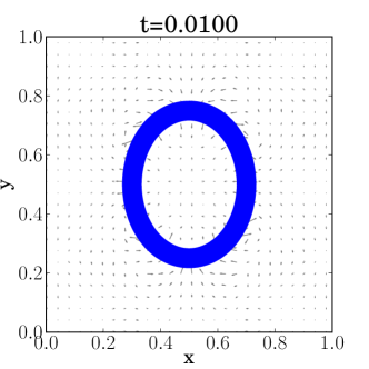
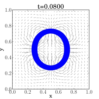
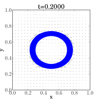
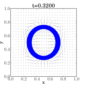
Figure 8: Snapshots of a thick oscillating ellipse using GM-IB method, with parameters $\mu=0.005$, $N=256$ and $\Delta t=0.08/512$.

Table 5: Estimated $\ell^{2}$ convergence rates ${\mathcal{R}}\left[q;128\right]$ for the thick ellipse problem at time $t=0.4$. For comparison, Griffith’s results [27] are reported in the final row. Since Griffith reports the component-wise convergence rate of the velocity field, we approximate ${\mathcal{R}}\left[\boldsymbol{u};128\right]\approx\max({\mathcal{R}}\left[u;128\right],~{}{\mathcal{R}}\left[v;128\right])$.

	$\mu=0.05$			$\mu=0.01$			$\mu=0.005$
	$\boldsymbol{u}$	$p$	$\boldsymbol{X}$	$\boldsymbol{u}$	$p$	$\boldsymbol{X}$	$\boldsymbol{u}$	$p$	$\boldsymbol{X}$
GM-IB	$2.10$	$1.88$	$1.69$	$2.12$	$1.88$	$1.76$	$2.11$	$1.88$	$1.99$
BCM-IB	$2.11$	$1.88$	$1.69$	$2.09$	$1.87$	$1.74$	$2.09$	$1.87$	$1.99$
Griffith [27]	$2.16^{*}$	$1.89$	$1.98$	–	–	–	$2.20^{*}$	$1.86$	$1.74$

Lastly, we investigate the accuracy with which our discrete solution satisfies the discrete divergence-free condition for a variety of time steps and spatial discretizations. Our aim in this instance is to determine how well the fluid solver of Guermond and Minev approximates the incompressibility constraint, which is related to the volume conservation issue discussed in the thin ellipse example. Table 6 lists values of the error in the discrete divergence of velocity, ${\mathcal{E}}\left[\nabla\cdot\boldsymbol{u};N\right]$, measured at time $t=0.4$ and estimated using equation (30). Observe that ${\mathcal{E}}\left[\nabla\cdot\boldsymbol{u};N\right]$ increases slightly as the spatial discretization is refined, but decreases when a smaller time step is used. This last result is to be expected because Guermond and Minev use a ${\mathcal{O}}\left(\Delta t\right)$ perturbation of the incompressibility constraint (8).

Table 6: Error in the divergence-free condition ${\mathcal{E}}\left[\nabla\cdot\boldsymbol{u};N\right]$ for the thick ellipse problem using the GM-IB method and $\mu=0.01$.

	$\Delta t=\frac{0.08}{512}$	$\Delta t=\frac{0.04}{512}$	$\Delta t=\frac{0.02}{512}$	$\Delta t=\frac{0.01}{512}$	$\Delta t=\frac{0.005}{512}$	$\Delta t=\frac{0.0025}{512}$
$N=64$	$6.34\text{e}{-3}$	$2.37\text{e}{-3}$	$8.93\text{e}{-4}$	$3.20\text{e}{-4}$	$1.08\text{e}{-4}$	$3.42\text{e}{-5}$
$N=128$	$8.94\text{e}{-3}$	$3.68\text{e}{-3}$	$1.49\text{e}{-3}$	$5.75\text{e}{-4}$	$2.11\text{e}{-4}$	$7.36\text{e}{-5}$
$N=256$	$1.00\text{e}{-2}$	$4.19\text{e}{-3}$	$1.73\text{e}{-3}$	$6.79\text{e}{-4}$	$2.55\text{e}{-4}$	$9.06\text{e}{-5}$
$N=512$	$1.04\text{e}{-2}$	$4.35\text{e}{-3}$	$1.80\text{e}{-3}$	$7.11\text{e}{-4}$	$2.68\text{e}{-4}$	$9.59\text{e}{-5}$

6 Parallel Performance Results

We now focus on comparing the parallel performance of our algorithm (GM-IB) with an analogous projection-based scheme (BCM-IB). We begin by comparing the performance difference between solving the pure Poisson problem that plays a central role in projection schemes, versus Guermond and Minev’s directional-split counterpart. This captures the major differences between the fluid solvers used in the corresponding IB algorithms. We then follow by performing weak and strong scalability tests for the full immersed boundary problem.

6.1 Comparison with Poisson Solvers

In this section, we compare the performance of several Poisson solvers with our tridiagonal solver described in section 4.2. Since any standard projection scheme requires solving a Poisson problem, this performance study encapsulates the major differences between Guermond and Minev’s fluid solver and other projection-based approaches (for example, that of Brown-Cortez-Minion). To illustrate the comparison, we consider the problem

$$\left\{\begin{array}[]{c l}\textbf{A}\psi=f(\boldsymbol{x})&\mbox{~{}in }\Omega=[0,1]^{d},\\ \psi\mbox{~{}is periodic }&\mbox{~{}on }\partial\Omega,\end{array}\right.$$ (36)

where

$$f(\boldsymbol{x})=\left\{\begin{array}[]{c l}\sin(2\pi x)\cos(2\pi y)&\mbox{~{}when }d=2,\\ \sin(2\pi x)\cos(2\pi y)\cos(2\pi z)&\mbox{~{}when }d=3,\\ \end{array}\right.$$

and A is either the Laplacian operator ($\textbf{A}=\nabla^{2}$) or the directional-split operator $\textbf{A}=(1-\partial_{xx})(1-\partial_{yy})$ (when $d=2$).

When solving the Poisson problem, we compare with two other solvers: one based on FFTs and the other on multigrid. For both of these solvers we discretize the problem using a second-order finite difference scheme. In the FFT-based solver, the difference scheme is rewritten in terms of the Fourier coefficients and solved using the real-to-complex and complex-to-real transformations found in FFTW [16]. For the multigrid solver, we use a highly scalable multigrid preconditioner (PFMG) implemented in Hypre [15] that is used with a conjugate gradient solver. When performing the comparison for the directional-split problem, the discrete system decouples into a set of one-dimensional tridiagonal systems that we solve using the techniques described in section 4.2. The major differences here occur in terms of the domain partitioning, which for the FFT-based solver involves a slab decomposition, whereas the multigrid and directional-split solvers use square-like subdomains.

Throughout our performance study, times are collected using MPI and the best result of multiple runs is reported. All simulations are performed using the Bugaboo cluster managed by WestGrid [63], a member of the high-performance computing consortium Compute Canada. This cluster consists of 12-core blades, each containing two Intel Xeon X5650 6-core processors (2.66 GHz) that are connected by Infiniband using a 288-port QLogic switch.

First, we evaluate the strong scaling property of each solver by running a sequence of simulations in which the problem size is held fixed as the number of processors increases. For the three-dimensional computations, the problems are solved on $N=128$ and $N=256$ grids, which are common resolutions used in 3D IB calculations. For the two-dimensional computations, the problems are solved on grids that are larger than usual ($N=2048$ and $4096$). The strong scaling results are given in Tables 7 and 8, which report the execution time $T_{P}$ and parallel efficiency

$$E_{P}=\frac{T_{1}}{PT_{P}},$$

for $P$ processors. The parallel efficiency quantifies how well the processors are utilized throughout a computation, where a value of $E_{P}=1$ corresponds to the ideal case and smaller values indicate a reduced parallel efficiency. Note that a reduction in efficiency is expected since the serial computation involves no Schur complement systems but instead computes the tridiagonal systems directly.

In all parallel computations, we observe that the directional-split solver is strongly scalable ($E_{P}>0.8$) and outperforms both Poisson solvers by a significant margin. Indeed, when comparing the directional-split solver to multigrid, there is an order of magnitude difference in execution time. For all multigrid computations, the conjugate gradient solver required $6$ iterations which makes the directional-split solver a factor of $2$ to $5$ times faster than a single multigrid iteration. When comparing the directional-split solver to the FFT-based solver, the difference in execution times is much smaller, particularly when using fewer processors. However, as the processor count increases, we still see a two-fold or greater performance improvement when using the directional-split solver.

Besides the performance improvements, the Guermond and Minev fluid solver has a few additional advantages over FFT-based fluid solvers. First of all, FFT-based solvers are restricted to periodic boundaries while the directional-split solver has no such restriction. For example, the Guermond-Minev fluid solver can inexpensively compute driven-cavity and (periodic) channel flows without the use of immersed boundaries [30]. Secondly, the slab decomposition used by many FFT libraries (such as FFTW) can lead to serious load-balancing issues in the immersed boundary context as indicated by Yau [64]. Note that this could be mitigated somewhat in 3D simulations by moving to a pencil decomposition that consequently allows for more processors to be used in the computation [52].

Table 7: Execution time $T_{P}$ and parallel efficiency $E_{P}$ for the 2D problem (36) on an $N^{2}$ grid with $P$ processors.

		Multigrid		FFT		Directional-Split
	$P$	$T_{P}$	$E_{P}$	$T_{P}$	$E_{P}$	$T_{P}$	$E_{P}$
$N=2048$	$1$	$4.26\text{e}{+0}$	$--$	$3.10\text{e}{-1}$	$--$	$2.77\text{e}{-1}$	$--$
	$8$	$6.66\text{e}{-1}$	$0.80$	$7.93\text{e}{-2}$	$0.49$	$3.77\text{e}{-2}$	$0.92$
	$16$	$3.07\text{e}{-1}$	$0.87$	$3.57\text{e}{-2}$	$0.54$	$1.82\text{e}{-2}$	$0.95$
	$32$	$1.72\text{e}{-1}$	$0.77$	$2.50\text{e}{-2}$	$0.39$	$8.78\text{e}{-3}$	$0.99$
	$64$	$8.30\text{e}{-2}$	$0.80$	$1.43\text{e}{-2}$	$0.34$	$4.40\text{e}{-3}$	$0.99$
	$128$	$4.33\text{e}{-2}$	$0.77$	$1.20\text{e}{-2}$	$0.20$	$2.45\text{e}{-3}$	$0.88$
$N=4096$	$1$	$1.38\text{e}{+1}$	$--$	$1.33\text{e}{+0}$	$--$	$1.09\text{e}{+0}$	$--$
	$8$	$3.18\text{e}{+0}$	$0.54$	$3.58\text{e}{-1}$	$0.47$	$1.54\text{e}{-1}$	$0.88$
	$16$	$1.83\text{e}{+0}$	$0.47$	$2.15\text{e}{-1}$	$0.39$	$7.86\text{e}{-2}$	$0.87$
	$32$	$8.92\text{e}{-1}$	$0.48$	$1.17\text{e}{-1}$	$0.36$	$4.06\text{e}{-2}$	$0.84$
	$64$	$4.84\text{e}{-1}$	$0.45$	$6.36\text{e}{-2}$	$0.33$	$2.03\text{e}{-2}$	$0.84$
	$128$	$2.23\text{e}{-1}$	$0.48$	$3.84\text{e}{-2}$	$0.27$	$9.62\text{e}{-3}$	$0.84$
	$256$	$1.05\text{e}{-1}$	$0.51$	$2.57\text{e}{-2}$	$0.20$	$5.22\text{e}{-3}$	$0.81$

Table 8: Execution time $T_{P}$ and parallel efficiency $E_{P}$ for the 3D problem (36) on an $N^{3}$ grid with $P$ processors.

		Multigrid		FFT		Directional-Split
	$P$	$T_{P}$	$E_{P}$	$T_{P}$	$E_{P}$	$T_{P}$	$E_{P}$
$N=128$	$1$	$2.77\text{e}{+0}$	$--$	$1.60\text{e}{-1}$	$--$	$2.05\text{e}{-1}$	$--$
	$8$	$4.68\text{e}{-1}$	$0.74$	$3.16\text{e}{-2}$	$0.63$	$2.65\text{e}{-2}$	$0.97$
	$16$	$2.38\text{e}{-1}$	$0.73$	$1.88\text{e}{-2}$	$0.53$	$1.35\text{e}{-2}$	$0.95$
	$32$	$1.40\text{e}{-1}$	$0.62$	$1.21\text{e}{-2}$	$0.42$	$6.75\text{e}{-3}$	$0.95$
	$64$	$7.48\text{e}{-2}$	$0.58$	$6.67\text{e}{-3}$	$0.38$	$3.50\text{e}{-3}$	$0.92$
	$128$	$5.67\text{e}{-2}$	$0.38$	$4.57\text{e}{-3}$	$0.27$	$1.88\text{e}{-3}$	$0.85$
$N=256$	$1$	$2.16\text{e}{+1}$	$--$	$1.43\text{e}{+0}$	$--$	$1.71\text{e}{+0}$	$--$
	$8$	$3.58\text{e}{+0}$	$0.75$	$2.68\text{e}{-1}$	$0.67$	$2.26\text{e}{-1}$	$0.95$
	$16$	$1.93\text{e}{+0}$	$0.70$	$1.53\text{e}{-1}$	$0.58$	$1.12\text{e}{-1}$	$0.95$
	$32$	$1.15\text{e}{+0}$	$0.59$	$8.63\text{e}{-2}$	$0.52$	$5.51\text{e}{-2}$	$0.97$
	$64$	$6.77\text{e}{-1}$	$0.50$	$5.48\text{e}{-2}$	$0.41$	$2.80\text{e}{-2}$	$0.95$
	$128$	$3.97\text{e}{-1}$	$0.42$	$3.43\text{e}{-2}$	$0.32$	$1.52\text{e}{-2}$	$0.88$
	$256$	$2.26\text{e}{-1}$	$0.37$	$2.35\text{e}{-2}$	$0.24$	$7.46\text{e}{-3}$	$0.90$

Next we report the weak scaling results for the multigrid solver and the directional-split solver as shown in Figure 9. In each set of computations, the local problem size $n^{d}$ (where $N=n\cdot P_{x}$) is held fixed as the number of processors is increased. In the ideal case, the execution time should stay constant so that the workload per processor does not change as the number of nodes increase. For 2D problems ($d=2$), the local grid resolution on each subdomain is either $n=128$ or 256, while for 3D problems ($d=3$) we use either $n=32$ or $64$.

As expected [4, 29], both solvers are weakly scalable since the execution time stays essentially constant as the problem size and number of processors increase. For the $n=128$ simulations, the execution time jumps suddenly at $P=25$, which is due to increased communication costs occurring between blades inside the same chassis. Since the blades in a chassis are connected through the same switch where multiple cores share the same connection, and since the work load per processor is so small, a noticeable jump appears as a result of resource contention.

When comparing the execution time between solvers, the directional-split solver is around $1.5$ to $5$ times faster than a single multigrid iteration. Since the multigrid solver requires $5$ to $6$ iterations of conjugate gradient, this results in an order of magnitude difference in the total execution time. Of course, this difference would be reduced by using a better initial guess in the multigrid solver which would in turn require fewer iterations.

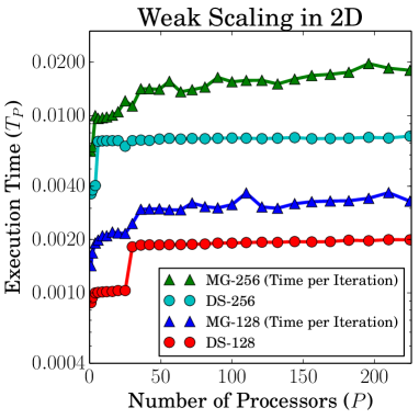
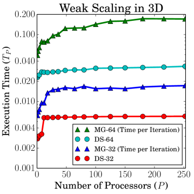
Figure 9: Weak scaling of the multigrid and directional-split solvers when approximating problem (36) in 2D and 3D. For the 2D computations, MG-128 and MG-256 denote the execution time of a single multigrid iterations using local $n=128$ and $256$ grids. Likewise, DS-128 and DS-256 denote the execution times for completely solving the directional-split problem. For 3D computations, we use a local $n=32$ and $n=64$ grids where the solver is specified using the same 2D naming convention.

As can be seen from this comparison, the directional-split solver outperformed the Poisson solvers in all non-serial computations. The precise difference depends on the problem size $N$, the number of processors $P$, and the hardware configuration of the cluster. Furthermore, when solving the Poisson problem, we used the two highly optimized libraries Hypre [15] and FFTW [16]. Therefore, we would expect to see even greater performance differences if we were to optimize the directional-split solver to the same degree as these other solvers.

6.2 Multiple Thin Ellipses in 2D

The next example is designed to explore in more detail the parallel performance of GM-IB and BCM-IB (with Hypre) by computing a variation of the thin ellipse problem from section 5.1. Because our 2D computations are performed on a doubly-periodic fluid domain, the thin ellipse geometry is actually equivalent to an infinite array of identical elliptical membranes. This periodicity in the solution provides a simple mechanism for increasing the computational complexity of a simulation by explicitly adding multiple periodic copies while technically solving a problem with a solution that is identical to that for a single membrane. Each copy of the original domain (see section 5.1) may then be handled by a different processing node, which allows us to explore the parallel performance in an idealized geometry.

Suppose that we would like to perform a parallel simulation using $P=P_{x}\cdot P_{y}$ processing nodes. On such a cluster, we can simulate a rectangular $P_{x}\times P_{y}$ array of identical ellipses, situated on the fluid domain $\Omega=[0,P_{x}]\times[0,P_{y}]$. We subdivide the domain into equal partitions so that each processor handles the unit-square subdomain $\Omega_{\ell,m}=[\ell-1,\ell]\times[m-1,m]$, for $\ell=1,2,\ldots,P_{x}$ and $m=1,2,\ldots P_{y}$. If we denote by $(x_{\ell,m},y_{\ell,m})$ the centroid of $\Omega_{\ell,m}$, then each such subdomain contains a single ellipse having the initial configuration

$$\boldsymbol{X}_{\ell,m}(s,0)=\left(x_{\ell,m}+r_{1}\cos(2\pi s),\;y_{\ell,m}+r_{2}\sin(2\pi s)\right),$$

where $s\in[0,1]$ is the same Lagrangian parameter as before. In order to make the flow slightly more interesting, and to test the ability of our parallel algorithm to handle immersed boundaries that move between processing nodes, we impose a constant background fluid velocity field $\boldsymbol{u}(\boldsymbol{x},0)=\frac{1}{2}\left(1,\sqrt{3}\right)$ instead of the zero initial velocity used in section 5.1. Snapshots of the solution for a $2\times 2$ array of ellipses are given in Figure 10.

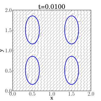
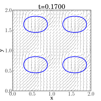
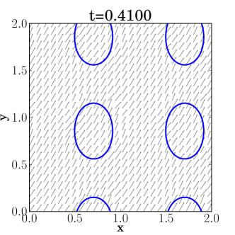
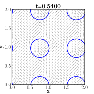
Figure 10: Simulation of a $2\times 2$ array of thin ellipses.

To investigate the parallel performance of the GM-IB and BCM-IB algorithms, we simulate different-sized arrays of thin ellipses corresponding to values of $P_{x}$ and $P_{y}$ in the range $[1,16]$. For each simulation, we use parameters $\mu=0.01$, $\rho=1$, $\sigma=1$, $r_{1}=\frac{5}{28}$, $r_{2}=\frac{7}{20}$, $h_{s}=\frac{4}{19}h$ and $\Delta t=0.01h$, and we compute up to time $t=1.00$ using two values of the fluid mesh width $h=\frac{1}{128}$ and $\frac{1}{256}$. In the case of perfect parallel scaling the execution time should remain constant between simulations, because of our problem constructon in which doubling the problem size also double the number of nodes $P$. Therefore, the problem represents a weak scalability test for our algorithm in which the workload per processor node remains constant as the number of nodes increase.

The execution times for various array sizes ($P_{x}$, $P_{y}$) are summarized in Figure 11 for both IB solvers. The execution time remains roughly constant in both cases, which indicates that the GM-IB and BCM-IB implementations are essentially weakly scalable. Notice that there is a slight degradation in performance as $P$ increases; for example, on the $h=\frac{1}{128}$ grid the GM-IB execution time increases by roughly $20\%$ between $P=64$ to $P=254$, which is minimal considering the large variation in problem size.

When comparing solvers, GM-IB outperforms BCM-IB by more than a factor of 5 in execution time. This difference in performance is largely due to the efficiency of the linear solvers. Here, the BCM-IB solver uses conjugate gradient with a multigrid preconditioner (PFMG) implemented within Hypre [15], where the initial guess is set to the solution from the previous time step. For this particular problem, the multigrid solver typically requires $2$ iterations to solve the momentum equations and $5$ iterations for the projection step. Naturally, if either iteration count could be reduced, the performance of the BCM-IB solver would improve significantly. However, since an iteration of multigrid is substantially slower than the directional-split solver (see section 6.1), GM-IB would continue to outperform BCM-IB.

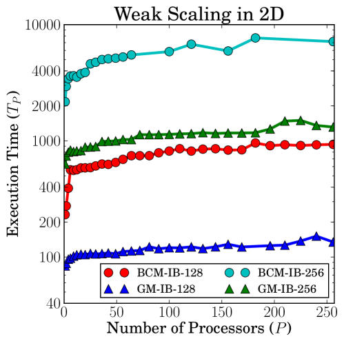
Figure 11: Execution time (in seconds) for the multiple thin ellipse problem using the BCM-IB and GM-IB algorithms ($P$ ellipses, $P$ processors, local grids with $n=128$ and $256$).

6.3 Cylindrical Shell in 3D

For our final test case, we consider a three-dimensional example in which the immersed boundary is a cylindrical elastic shell. The cylinder initially has an elliptical cross-section with semi-axes $r_{1}$ and $r_{2}$ that is parameterized by

$$\boldsymbol{X}(s,r,0)=\left(r,~{}\frac{1}{2}+r_{1}\cos(2\pi s),~{}\frac{1}{2}+r_{2}\sin(2\pi s)\right),$$

using the two Lagrangian parameters $s,r\in[0,1]$. The force density is

$$\boldsymbol{\mathcal{F}}[\boldsymbol{X}(s,r,t)]=\sigma_{s}\frac{\partial^{2}\boldsymbol{X}}{\partial s^{2}}+\sigma_{r}\frac{\partial}{\partial r}\left(\frac{\partial\boldsymbol{X}}{\partial r}\left(1-\frac{L}{\left|\frac{\partial\boldsymbol{X}}{\partial r}\right|}\right)\right),$$

which corresponds to an elastic shell made up of an interwoven mesh of one-dimensional elastic fibers. The $s$ parameterization identifies individual fibers running around the elliptical cross-section of the cylinder, each having zero resting length and elastic stiffness $\sigma_{s}$. On the other hand, the $r$ parameterization describes fibers running axially along the length of the cylinder, each having a non-zero resting-length $L$ and stiffness $\sigma_{r}$. Since the domain is periodic in all directions, the ends of the cylinder are connected to their periodic copies so that there are no “cuts” along the fibers. This problem is essentially equivalent to the two-dimensional thin ellipse problem considered in section 5.1, with the only difference being that the 2D problem does not have any fibers running along the non-existent third dimension. The 2D thin ellipse and 3D cylinder problems are only strictly equivalent when $\sigma_{r}=0$. However, we take $\sigma_{r}=\sigma_{s}=1$ and $L=1$ in order to maintain the integrity of the elastic shell and to avoid any drifting of elliptical cross-sections in the $x$-direction. The elastic shell is discretized using equally-spaced values of the Lagrangian parameters $s$ and $r$. In the simulations that follow, we use the parameter values $\mu=0.01$, $\rho=1$, $r_{1}=\frac{5}{28}$, $r_{2}=\frac{7}{20}$, $N_{s}=\frac{19}{4}N$, $N_{r}=3N$ and $\Delta t=0.04/N$ where $N=128$ and $N=256$.

The solution dynamics are illustrated by the snapshots pictured in Figure 12, and we observe that the 3D elastic shell oscillates at roughly the same frequency as the 2D ellipse shown in Figure 6. Although the geometry of this problem may seem somewhat of a special case because of the alignment of axial fibers along the $x$-coordinate direction, this feature has no noticeable impact on parallel performance measurements. Indeed, the reason that fiber alignment doesn’t affect communication cost is because all IB points and force connections residing in the ghost region are communicated regardless of whether or not they actually cross subdomain boundaries.

In Table 9, we present measurements of execution time and efficiency that illustrate the parallel scaling over the first $100$ time steps with the number of processors $P$ varying between 1 and 128. In all runs, the domain is partitioned evenly between the $P$ processing nodes using rectangular boxes. When the IB points are evenly distributed between all domain partitions, we observe good parallel efficiency. On average, we obtain a speedup factor of $1.85$ when doubling the number of processors for this particular problem.

For larger runs, the parallel efficiency does deteriorate as the local subdomain shrinks in size. For example, when subdividing a $N=128$ grid to a $(P_{x},P_{y},P_{z})=(32,2,2)$ array of processors, the local grid size is $4\times 64\times 64$. Therefore, every processor has to communicate all data within its subdomain to neighbouring processors, since the entire domain overlaps with ghost regions. For this reason, the GM-IB algorithm performs remarkably well, given the circumstances.

Lastly, in Table 9, we show the execution time for situations where the immersed boundary is not evenly distributed between processors. Since no load balancing strategy is incorporated in our implementation, the parallel efficiency drops as the computational work becomes more unevenly divided. Here, the total execution time becomes increasingly dominated by the IB portion of the calculation as the workload becomes more unbalanced. The parallel efficiency in this situation could be improved by partitioning the fluid domain in a dynamic manner, such as is done by IBAMR using SAMRAI in [25].

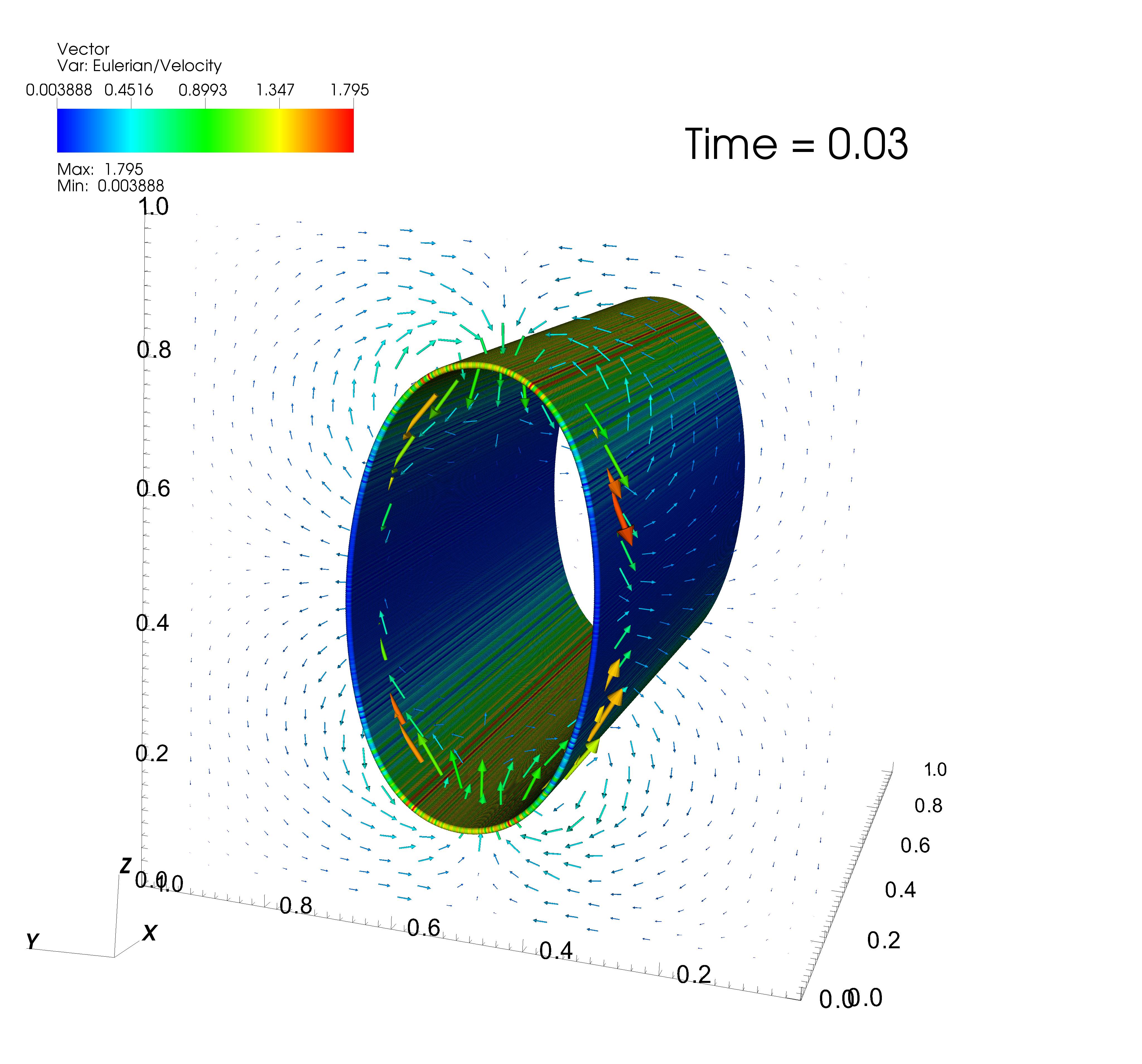
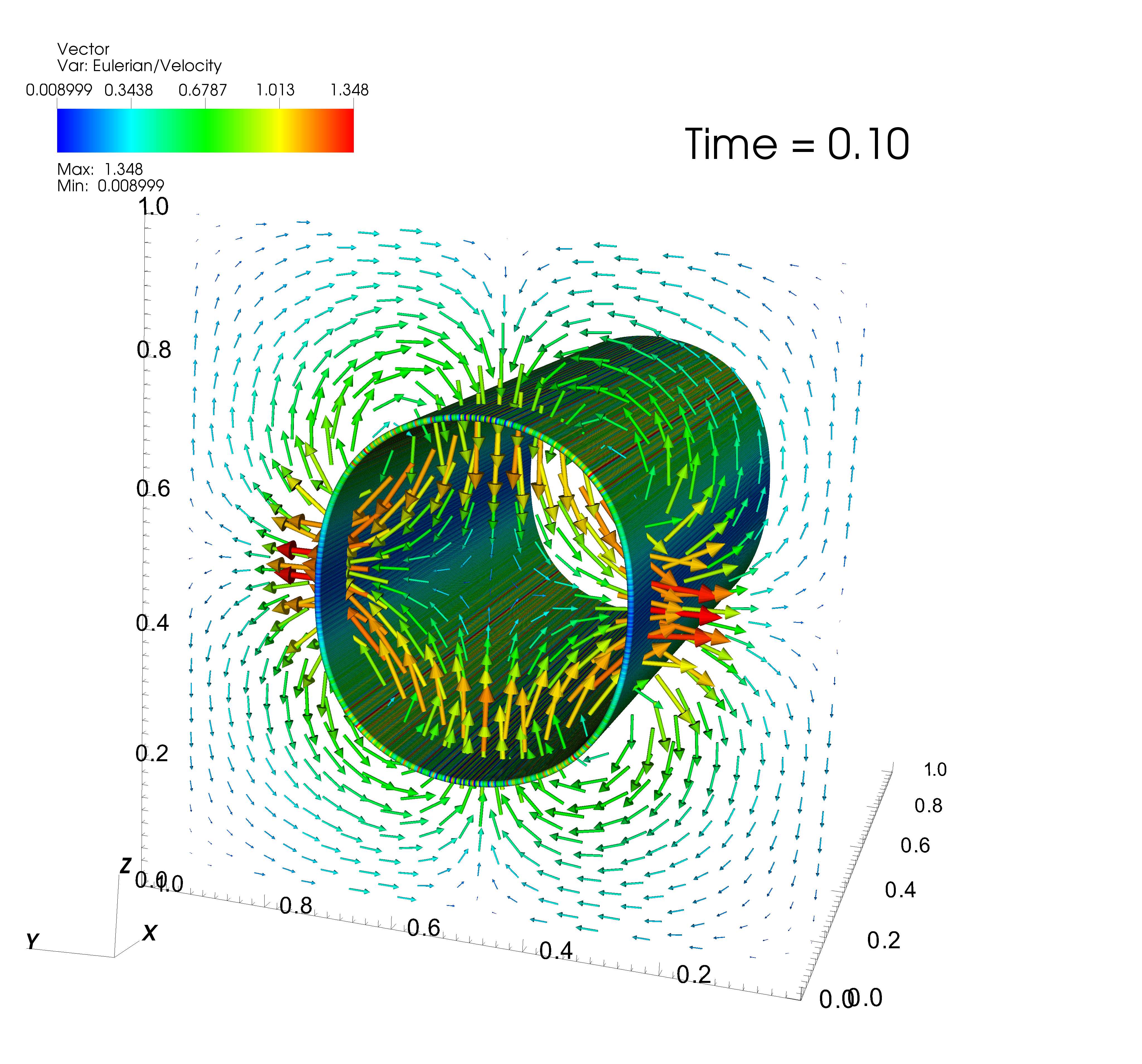
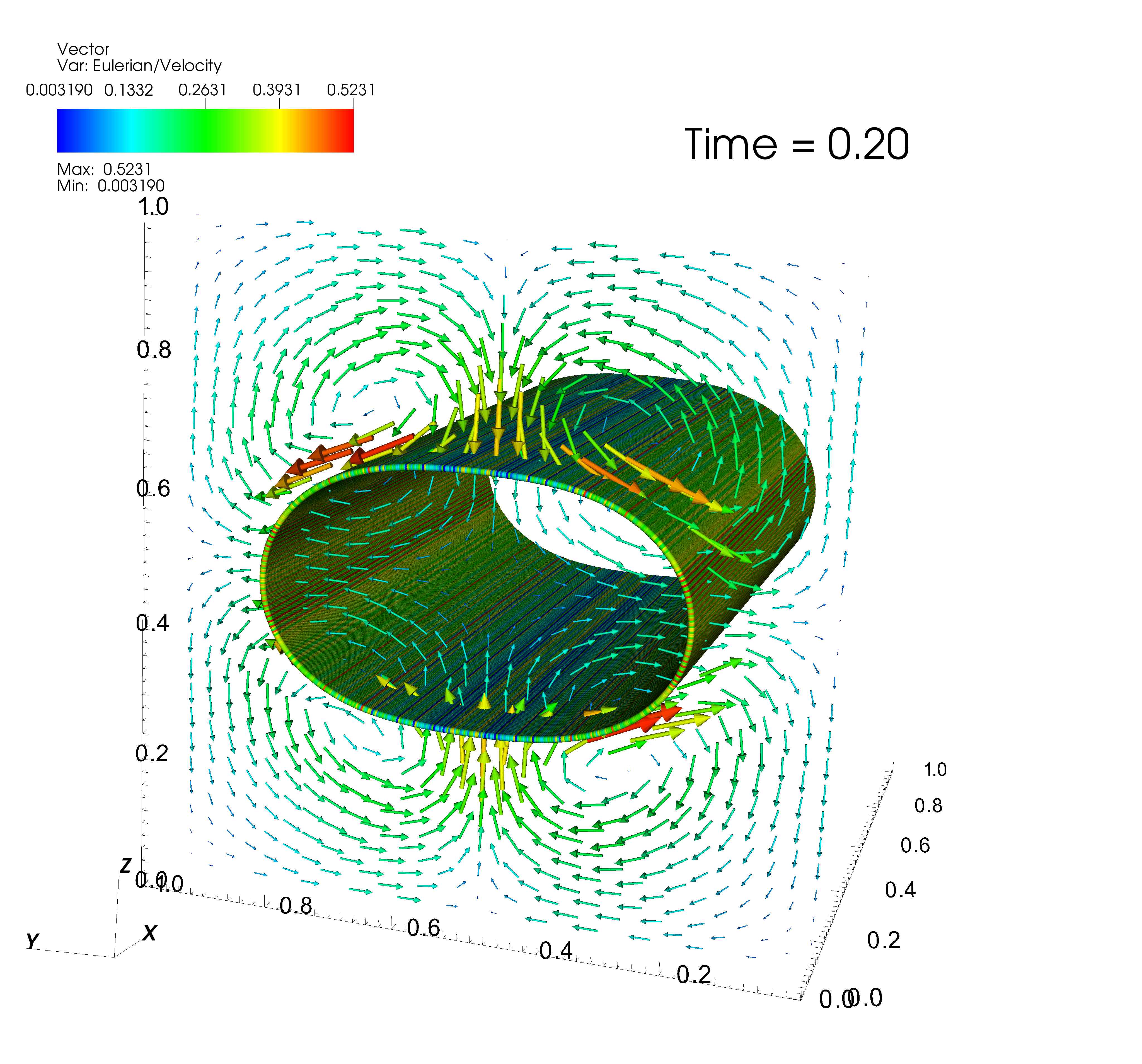
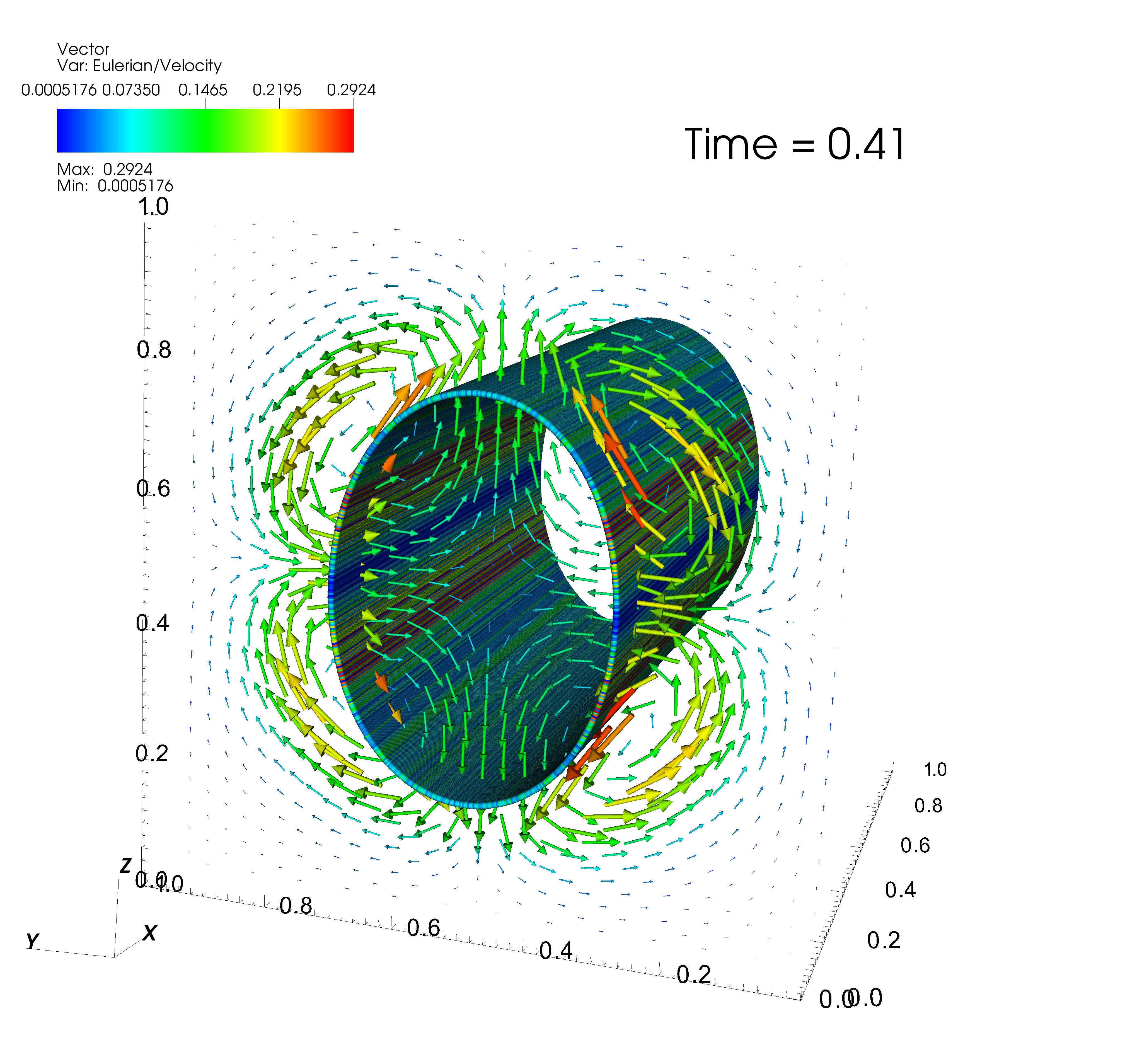
Figure 12: Snapshots of an oscillating 3D cylindrical shell ($N=128$) that is initially stretched outward along the $x$–direction.

Table 9: Execution time (in seconds) and efficiency for the 3D cylindrical shell problem for a fixed problem size while varying the number of processing nodes $P$.

		$N=128$		$N=256$
$P$	($P_{x},P_{y},P_{z}$)	Wall Time	Efficiency	Wall Time	Efficiency
$1$	($1,1,1$)	$4.01\text{e}{+2}$	$1.00$	$2.60\text{e}{+3}$	$1.00$
$2$	($2,1,1$)	$2.11\text{e}{+2}$	$0.93$	$1.43\text{e}{+3}$	$0.91$
$4$	($4,1,1$)	$1.18\text{e}{+2}$	$0.81$	$7.06\text{e}{+2}$	$0.92$
$8$	($2,2,2$)	$6.07\text{e}{+1}$	$0.82$	$3.52\text{e}{+2}$	$0.92$
$16$	($4,2,2$)	$3.18\text{e}{+1}$	$0.82$	$1.83\text{e}{+2}$	$0.89$
$32$	($8,2,2$)	$1.65\text{e}{+1}$	$0.79$	$9.64\text{e}{+1}$	$0.84$
$64$	($16,2,2$)	$9.42\text{e}{+0}$	$0.70$	$5.39\text{e}{+1}$	$0.75$
$128$	($32,2,2$)	$7.76\text{e}{+0}$	$0.55$	$3.02\text{e}{+1}$	$0.67$
$32$	($4,4,2$)	$2.53\text{e}{+1}$	$0.52$	$1.30\text{e}{+2}$	$0.62$
$64$	($4,4,4$)	$1.42\text{e}{+1}$	$0.46$	$7.13\text{e}{+1}$	$0.57$
$128$	($8,4,4$)	$7.76\text{e}{+0}$	$0.42$	$3.72\text{e}{+1}$	$0.55$

7 Conclusions

We have developed a new algorithm for the immersed boundary problem on distributed-memory parallel computers that is based on the pseudo-compressibility method of Guermond and Minev for solving the incompressible Navier-Stokes equations. The fundamental advantage of this fluid solver is the direction-splitting strategy applied to the incompressibility constraint, which reduces to solving a series of tridiagonal linear systems with an extremely efficient parallel implementation.

Numerical computations demonstrate the ability of our method to simulate a wide range of immersed boundary problems that includes not only 2D flows containing isolated fibers and thick membranes constructed of multiple nested fibers, but also 3D flows containing immersed elastic surfaces. The strong and weak scalability of our algorithm is demonstrated in tests with up to 256 distributed processors, where excellent speedups are observed. Furthermore, comparisons against FFT-based (FFTW [16]) and multigrid (Hypre [15]) solvers shows substantial performance improvements when using the Guermond and Minev solver. We observe that since our implementation does not apply any load balancing strategy, some degradation in the parallel efficiency is observed in immersed boundary portion of the computation when the elastic membrane is not equally divided between processors.

We believe that our computational approach is a promising one for solving fluid-structure interaction problems in which the solid elastic component takes up a large portion of the fluid domain, such as occurs with dense particle suspensions [60] or very complex elastic structures that are distributed throughout the fluid. These are problems where local adaptive mesh refinement is less likely to offer any advantage because of the need to use a nearly-uniform fine mesh over the entire domain in order to resolve the immersed boundary. It is for this class of problems that we expect our approach to offer significant advantages over methods such as that of Griffith et al. [24].

We plan in future to implement modifications to our algorithm that will improve the parallel scaling, and particularly on improving memory access patterns for the Lagrangian portion of the calculation related to force spreading and velocity interpolation. We will also investigate code optimizations that aim to reduce cache misses and exploit on-chip parallelism. Lastly, work has started on applying this algorithm to study spherical membrane dynamics, particle sedimentation, and fiber suspensions.

References

- [1] P. Angot, J. Keating, and P. D. Minev. A direction splitting algorithm for incompressible flow in complex geometries. Computer Methods in Applied Mechanics and Engineering, 217:111–120, 2012.
- [2] K. Asanovic, R. Bodik, B. C. Catanzaro, J. J. Gebis, P. Husbands, K. Keutzer, D. A. Patterson, W. L. Plishker, J. Shalf, and S. W. Williams. The landscape of parallel computing research: A view from Berkeley. Technical report, UCB/EECS-2006-183, EECS Department, University of California, Berkeley, 2006.
- [3] K. Asanovic, R. Bodik, J. Demmel, T. Keaveny, K. Keutzer, J. Kubiatowicz, N. Morgan, D. Patterson, K. Sen, and J. Wawrzynek. A view of the parallel computing landscape. Communications of the ACM, 52(10):56–67, 2009.
- [4] A. H. Baker, R. D. Falgout, T. V. Kolev, and U. M. Yang. Scaling hypre’s multigrid solvers to 100,000 cores. In High-Performance Scientific Computing, pages 261–279. Springer, 2012.
- [5] S. Balay, J. Brown, K. Buschelman, V. Eijkhout, W. Gropp, D. Kaushik, M. Knepley, L. C. McInnes, B. Smith, and H. Zhang. PETSc Users Manual, Revision 3.3. Report ANL-95/11, Mathematics and Computer Science Division, Argonne National Laboratory, Argonne, IL, June 2012. Retrieved April 28, 2013 from http://www.mcs.anl.gov/petsc/documentation/index.html.
- [6] T. T. Bringley and C. S. Peskin. Validation of a simple method for representing spheres and slender bodies in an immersed boundary method for Stokes flow on an unbounded domain. Journal of Computational Physics, 227:5397–5425, 2008.
- [7] D. L. Brown, R. Cortez, and M. L. Minion. Accurate projection methods for the incompressible Navier–Stokes equations. Journal of Computational Physics, 168(2):464–499, 2001.
- [8] H. D. Ceniceros, J. E. Fisher, and A. M. Roma. Efficient solutions to robust, semi-implicit discretizations of the immersed boundary method. Journal of Computational Physics, 228(19):7137–7158, 2009.
- [9] A. J. Chorin. A numerical method for solving incompressible viscous flow problems. Journal of Computational Physics, 2(1):12–26, 1967.
- [10] A. J. Chorin. Numerical solution of the Navier-Stokes equations. Mathematics of Computation, 22(104):745–762, 1968.
- [11] P. Colella. Multidimensional upwind methods for hyperbolic conservation laws. Journal of Computational Physics, 87(1):171–200, 1990.
- [12] R. H. Dillon, L. J. Fauci, C. Omoto, and X. Yang. Fluid dynamic models of flagellar and ciliary beating. Annals of the New York Academy of Sciences, 1101(1):494–505, 2007.
- [13] J. Douglas. Alternating direction methods for three space variables. Numerische Mathematik, 4:41–63, 1962.
- [14] C. Duncan, G. Zhai, and R. Scherer. Modeling coupled aerodynamics and vocal fold dynamics using immersed boundary methods. Acoustical Society of America Journal, 120(5):2859–2871, 2006.
- [15] R. D. Falgout, J. E. Jones, and U. M. Yang. The design and implementation of hypre, a library of parallel high performance preconditioners. In Numerical solution of partial differential equations on parallel computers, pages 267–294. Springer, 2006.
- [16] M. Frigo and S. G. Johnson. FFTW: An adaptive software architecture for the FFT. In Proceedings of the 1998 IEEE International Conference on Acoustics, Speech, and Signal Processing., volume 3, pages 1381–1384. IEEE, 1998.
- [17] E. Gabriel, G. E. Fagg, G. Bosilca, T. Angskun, J. J. Dongarra, J. M. Squyres, V. Sahay, P. Kambadur, B. Barrett, A. Lumsdaine, R. H. Castain, D. J. Daniel, R. L. Graham, and T. S. Woodall. Open MPI: Goals, concept, and design of a next generation MPI implementation. In Proceedings, 11th European PVM/MPI Users’ Group Meeting, pages 97–104, Budapest, Hungary, September 2004.
- [18] M. Ganzha, K. Georgiev, I. Lirkov, S. Margenov, and M. Paprzycki. Highly parallel alternating directions algorithm for time dependent problems. In Third Conference on Application of Mathematics in Technical and Natural Sciences, volume 1404 of AIP Conference Proceedings, pages 210–217, Albena, Bulgaria, June 20-25, 2011.
- [19] E. Givelberg and K. Yelick. Distributed immersed boundary simulation in Titanium. SIAM Journal on Scientific Computing, 28(4):1361–1378, 2006.
- [20] S. Gottlieb, C. W. Shu, and E. Tadmor. Strong stability-preserving high-order time discretization methods. SIAM Review, 43(1):89–112, 2001.
- [21] B. E. Griffith. Simulating the blood-muscle-valve mechanics of the heart by an adaptive and parallel version of the immersed boundary method. PhD thesis, New York University, 2005.
- [22] B. E. Griffith. An accurate and efficient method for the incompressible Navier-Stokes equations using the projection method as a preconditioner. Journal of Computational Physics, 228(20):7565–7595, 2009.
- [23] B. E. Griffith. On the volume conservation of the immersed boundary method. Communications in Computational Physics, 12:401–432, 2012.
- [24] B. E. Griffith, R. D. Hornung, D. M. McQueen, and C. S. Peskin. An adaptive, formally second order accurate version of the immersed boundary method. Journal of Computational Physics, 223(1):10–49, 2007.
- [25] B. E. Griffith, R. D. Hornung, D. M. McQueen, and C. S. Peskin. Parallel and adaptive simulation of cardiac fluid dynamics. In M. Parashar and X. Li, editors, Advanced computational infrastructures for parallel and distributed adaptive application, pages 105–130. John Wiley and Sons, 2009.
- [26] B. E. Griffith, X. Y. Luo, D. M. McQueen, and C. S. Peskin. Simulating the fluid dynamics of natural and prosthetic heart valves using the immersed boundary method. International Journal of Applied Mechanics, 1(1):137–177, 2009.
- [27] B. E. Griffith and C. S. Peskin. On the order of accuracy of the immersed boundary method: Higher order convergence rates for sufficiently smooth problems. Journal of Computational Physics, 208(1):75–105, 2005.
- [28] J. L. Guermond and P. D. Minev. A new class of fractional step techniques for the incompressible Navier-Stokes equations using direction splitting. Comptes Rendus Mathematique, 348:581–585, 2010.
- [29] J. L. Guermond and P. D. Minev. A new class of massively parallel direction splitting for the incompressible Navier-Stokes equations. Computer Methods in Applied Mechanics and Engineering, 200(23-24):2083–2093, 2011.
- [30] J. L. Guermond and P. D. Minev. Start-up flow in a three-dimensional lid-driven cavity by means of a massively parallel direction splitting algorithm. International Journal for Numerical Methods in Fluids, 68(7):856–871, 2011.
- [31] J. L. Guermond, P. D. Minev, and A. J. Salgado. Convergence analysis of a class of massively parallel direction splitting algorithms for the Navier-Stokes equations in simple domains. Mathematics of Computation, 81(280):1951, 2012.
- [32] C. Hamlet, A. Santhanakrishnan, and L. A. Miller. A numerical study of the effects of bell pulsation dynamics and oral arms on the exchange currents generated by the upside-down jellyfish Cassiopea xamachana. Journal of Experimental Biology, 214:1911–1921, 2011.
- [33] F. H. Harlow and J. E. Welch. Numerical calculation of time-dependent viscous incompressible flow of fluid with free surface. Physics of Fluids, 8(12):2182–2189, 1965.
- [34] T. Y. Hou and Z. Shi. An efficient semi-implicit immersed boundary method for the Navier-Stokes equations. Journal of Computational Physics, 227(20):8968–8991, 2008.
- [35] IBAMR: An adaptive and distributed-memory parallel implementation of the immersed boundary (IB) method. Retrieved April 28, 2013 from http://code.google.com/p/ibamr.
- [36] M. C. Lai and C. S. Peskin. An immersed boundary method with formal second-order accuracy and reduced numerical viscosity. Journal of Computational Physics, 160(2):705–719, 2000.
- [37] D. V. Le, J. White, J. Peraire, K. M. Lim, and B. C. Khoo. An implicit immersed boundary method for three-dimensional fluid-membrane interactions. Journal of Computational Physics, 228(22):8427–8445, 2009.
- [38] L. Lee and R. J. LeVeque. An immersed interface method for incompressible Navier–Stokes equations. SIAM Journal on Scientific Computing, 25(3):832–856, 2003.
- [39] R. J. LeVeque and Z. Li. Immersed interface methods for Stokes flow with elastic boundaries or surface tension. SIAM Journal on Scientific Computing, 18(3):709–735, 1997.
- [40] P. McCorquodale, P. Colella, and H. Johansen. A Cartesian grid embedded boundary method for the heat equation on irregular domains. Journal of Computational Physics, 173(2):620–635, 2001.
- [41] L. A. Miller and C. S. Peskin. Computational fluid dynamics of ‘clap and fling’ in the smallest insects. Journal of Experimental Biology, 208:195–212, 2005.
- [42] M. L. Minion. On the stability of Godunov-projection methods for incompressible flow. Journal of Computational Physics, 123(2):435–449, 1996.
- [43] R. Mittal and G. Iaccarino. Immersed boundary methods. Annual Review of Fluid Mechanics, 37:239–261, 2005.
- [44] Y. Mori and C. S. Peskin. Implicit second-order immersed boundary methods with boundary mass. Computer Methods in Applied Mechanics and Engineering, 197(25–28):2049–2067, 2008.
- [45] Y. Morinishi, T. Lund, O. Vasilyev, and P. Moin. Fully conservative higher order finite difference schemes for incompressible flow. Journal of Computational Physics, 143(1):90–124, 1998.
- [46] E. P. Newren. Enhancing the immersed boundary method: Stability, volume conservation, and implicit solvers. PhD thesis, Department of Mathematics, University of Utah, Salt Lake City, UT, May 2007.
- [47] E. P. Newren, A. L. Fogelson, R. D. Guy, and R. M. Kirby. Unconditionally stable discretizations of the immersed boundary equations. Journal of Computational Physics, 222(2):702–719, 2007.
- [48] E. P. Newren, A. L. Fogelson, R. D. Guy, and R. M. Kirby. A comparison of implicit solvers for the immersed boundary equations. Computer Methods in Applied Mechanics and Engineering, 197(25-28):2290–2304, 2008.
- [49] C. S. Peskin. Flow patterns around heart valves: A numerical method. Journal of Computational Physics, 10:252–271, 1972.
- [50] C. S. Peskin. The immersed boundary method. Acta Numerica, 11:479–517, 2002.
- [51] C. S. Peskin and B. F. Printz. Improved volume conservation in the computation of flows with immersed elastic boundaries. Journal of Computational Physics, 105:33–46, 1993.
- [52] M. Pippig. PFFT: An extension of FFTW to massively parallel architectures. SIAM Journal on Scientific Computing, 35(3):C213–C236, 2013.
- [53] R. Rannacher. On Chorin’s projection method for the incompressible Navier-Stokes equations. In J. Heywood, K. Masuda, R. Rautmann, and V. Solonnikov, editors, The Navier-Stokes Equations II – Theory and Numerical Methods, volume 1530 of Lecture Notes in Mathematics, pages 167–183. Springer, Berlin/Heidelberg, 1992.
- [54] Y. Saad. Iterative Methods for Sparse Linear Systems, volume 620. PWS Publishing Company, Boston, 1996.
- [55] J. Shen. On a new pseudo-compressibility method for the incompressible Navier-Stokes equations. Applied Numerical Mathematics, 21:71–90, 1996.
- [56] J. Shen. Pseudo-compressibility methods for the unsteady incompressible Navier-Stokes equations. In Proceedings of the 1994 Beijing Symposium on Nonlinear Evolution Equations and Infinite Dynamical Systems, pages 68–78, 1997.
- [57] J. M. Stockie. Analysis and Computation of Immersed Boundaries, with Application to Pulp Fibres. PhD thesis, Institute of Applied Mathematics, University of British Columbia, Vancouver, Canada, 1997. Available from https://circle.ubc.ca/handle/2429/7346.
- [58] J. M. Stockie and B. R. Wetton. Analysis of stiffness in the immersed boundary method and implications for time-stepping schemes. Journal of Computational Physics, 154(1):41–64, 1999.
- [59] R. Temam. Une méthode d’approximation de la solution des équations de Navier-Stokes. Bulletin de la Société Mathématique de France, 98(4):115–152, 1968.
- [60] A.-K. Tornberg and M. J. Shelley. Simulating the dynamics and interactions of flexible fibers in Stokes flows. Journal of Computational Physics, 196:8–40, 2004.
- [61] E. Twizell, A. Gumel, and M. Arigu. Second-order, L0-stable methods for the heat equation with time-dependent boundary conditions. Advances in Computational Mathematics, 6:333–352, 1996.
- [62] M. Uhlmann. Simulation of particulate flows on multi-processor machines with distributed memory. Technical Report 1039, CIEMAT, Madrid, Spain, May 2003.
- [63] WestGrid. QuickStart Guide to Bugaboo. Retrieved April 11, 2013 from http://www.westgrid.ca/support/quickstart/bugaboo.
- [64] S. M. Yau. Experiences in using titanium for simulation of immersed boundary biological systems. Master’s thesis, UC Berkeley, 2002.