Dynamically Disordered Quantum Walk as a Maximal Entanglement Generator

Abstract

We show that the entanglement between the internal (spin) and external (position) degrees of freedom of a qubit in a random (dynamically disordered) one-dimensional discrete time quantum random walk (QRW) achieves its maximal possible value asymptotically in the number of steps, outperforming the entanglement attained by using ordered QRW. The disorder is modeled by introducing an extra random aspect to QRW, a classical coin that randomly dictates which quantum coin drives the system’s time evolution. We also show that maximal entanglement is achieved independently of the initial state of the walker, study the number of steps the system must move to be within a small fixed neighborhood of its asymptotic limit, and propose two experiments where these ideas can be tested.

Introduction. Imagine we have a qubit, a quantum particle that in addition to its external degrees of freedom (position and momentum) has a spin-1/2-like internal one (two level system) mudanca1 . We assume it evolves in time as follows. We first apply a unitary operation $C$ (our “quantum coin”) acting only on the qubit’s internal degree of freedom, leaving it generally in a superposition of spin up and down. We then apply another unitary operation $S$ that correlates the displacement of the qubit to its internal degree of freedom. It moves right if the spin state at a given site is up and left otherwise. In this way we entangle the internal and external degrees of freedom of the system. Successive applications of the previous procedure lead to the discrete time evolution (displacement) of the qubit. This is what we call the one-dimensional discrete time quantum random walk (QRW) aha93 ; kem03 .

The key difference between the classical random walk (CRW) per05ray05 and QRW is the superposition principle of quantum mechanics, a feature that is obviously lacking in CRW. The application of $C$ followed by the displacement operator $S$ at each step generates a cat-like state among all possible positions of the particle, setting the stage for interference effects to take place. The interference among the probability amplitudes manifests itself producing a position probability distribution $P(j)$ drastically different from the classical one. Indeed, $P(j)$ for the unbiased CRW is always peaked about the initial position and drops off exponentially with the square of the distance (Gaussian distribution). Also, its variance $\sigma^{2}$ is proportional to the number $n$ of steps (coins flipped). This is the diffusive behavior. For the unbiased QRW, however, $P(j)$ is roughly uniform as we move away from the origin, having peaks far from it. Moreover, depending on the initial spin state we can have one peak at the left, or at the right, or two symmetrical peaks kem03 , and $\sigma^{2}\propto n^{2}$, a quadratic gain (ballistic behavior) in the propagation of the particle when compared to CRW. Furthermore, due to the $SU(2)$ structure of $C$, we have a coin with three independent parameters while classically there is only one.

Both CRW and QRW, in the one or higher dimensional versions, have many important applications application . And the majority of studies dealing with QRW assume that $C$ is the same during all steps of the walk or changes in a deterministic way kem03 ; she03 ; eng07 ; chi09 ; lov10 ; car05 ; bos09 . What would happen, though, if noise, disorder, or fluctuations change $C$ from one step to the other? What would happen if $C$ changes randomly between two possible coins? A naive guess would suggest that all features of QRW may be washed out by such a process. Indeed, it is known that some typical features of QRW, such as $P(j)$ and $\sigma^{2}$, change in such random processes and approach the classical case rib04 . However, so far no systematic numerical and/or analytical studies along this line were done for the entanglement content of the walker and for any initial condition. The only exception is Ref. cha12 , which came to our knowledge after finishing this work, and where for only one initial condition and a particular type of static and dynamical disorder the behavior of entanglement was numerically investigated for a 100-step walk.

Our main goal here is to investigate such extra random aspect on a quantum random walk (QRW) and analyze whether or not it is detrimental to its entanglement generation capacity. And our main finding is, surprisingly, that the opposite from the naive guess occurs when it comes to entanglement generation using a dynamically disordered QRW. We show that the entanglement, a genuine quantum feature, between the internal and external degrees of freedom of the walker is enhanced when $C$ changes from one step to the other in a truly random way. We also show that we achieve, asymptotically in the number of steps, a maximally entangled state. Moreover, we show that this effect is independent of the initial condition, contrary to standard entanglement generation schemes that rely critically on the initial state of the system and never achieve maximal entanglement car05 . It is worth mentioning that this initial state independence that we show here has important practical consequences and shows that the entanglement generation scheme here presented is robust against imperfections in the preparation of the initial state.

In order to explore these ideas we introduce a walker that combines the features of both the classical and quantum ones in a single formalism. It has two random ingredients, one of which is a classical coin similar to that of CRW. This coin dictates which quantum coin (the source of position randomness) will be used at each step of the walk. This is the essence of this walker and the presence of these two different random aspects, one classical and another quantum, leads us to call it a random quantum random walk (RQRW) process. We show in Appendix A that CRW and QRW are two particular cases of RQRW. Note that the quantum random aspect manifests itself only when we measure the position or spin of the walker (measurement postulate of quantum mechanics). The dynamics is unitary, however, leading some authors to call the ordered case simply QW instead of QRW.

Mathematical formalism. The Hilbert space of RQRW is $\mathcal{H}=\mathcal{H}_{C}\otimes\mathcal{H}_{P}$, where $\mathcal{H}_{C}$ is a two-dimensional complex vector space associated to the spin states $\{|\!\uparrow\rangle,|\!\downarrow\rangle\}$ and $\mathcal{H}_{P}$ is an infinite-dimensional but countable complex Hilbert space spanned by all integers. Its base is represented by the kets $|j\rangle$, $j\in\mathbb{Z}$, and they denote the position of the qubit on the lattice. With this notation we write an arbitrary initial state of the qubit (walker) as $|\Psi(0)\rangle=\sum_{j}(a(j,0)|\!\uparrow\rangle$ $\otimes|j\rangle+b(j,0)|\!\downarrow\rangle\otimes|j\rangle),$ with $\sum_{j}(|a(j,0)|^{2}+|b(j,0)|^{2})=1$ being the normalization condition and $j$ running over all integers. The time $t$ is discrete and it denotes the steps of the walker. In a $n$-step process the time changes from $t=0$ to $t=n$ in increments of one and the walker’s state is $|\Psi(n)\rangle=U(n)\cdots U(1)|\Psi(0)\rangle=\mathcal{T}\prod_{t=1}^{n}U(t)|\Psi(0)\rangle,$ where $\mathcal{T}$ denotes a time-ordered product, and

$$U(t)=S(C(t)\otimes\mathbb{1}_{P}).$$ (1)

Here $\mathbb{1}_{P}$ is the identity operator acting on the space $\mathcal{H}_{P}$, $C(t)$ the time-dependent quantum coin, and $S$ the conditional displacement operator. The operator $S$ moves the qubit at site $j$ to the site $j+1$ if its spin is up and to the site $j-1$ if its spin is down. Using the present notation $S=\sum_{j}(|\!\uparrow\rangle\langle\uparrow\!|\otimes|j+1\rangle\langle j|+|\!\downarrow\rangle\langle\downarrow\!|\otimes|j-1\rangle\langle j|).$

An arbitrary $C(t)$ is given by the most general way of writing an $SU(2)$ unitary transformation. Up to an irrelevant global phase we have $C(t)=c_{\uparrow\uparrow}(t)$ $|\uparrow\rangle\langle\uparrow|+c_{\uparrow\downarrow}(t)|\uparrow\rangle\langle\downarrow|+c_{\downarrow\uparrow}(t)|\downarrow\rangle\langle\uparrow|+c_{\downarrow\downarrow}(t)|\downarrow\rangle\langle\downarrow|,$ with $c_{\uparrow\uparrow}(t)=\sqrt{q(t)}$, $c_{\uparrow\downarrow}(t)=\sqrt{1-q(t)}e^{i\theta(t)}$, $c_{\downarrow\uparrow}(t)=\sqrt{1-q(t)}e^{i\varphi(t)}$, and $c_{\downarrow\downarrow}(t)=-\sqrt{q(t)}e^{i(\theta(t)+\varphi(t))}$. Here $0\leq q(t)\leq 1$ and $0\leq\theta(t),\varphi(t)\leq 2\pi$. The first parameter controls the bias of $C(t)$. For $q(t)=1/2$ the coin creates an equal superposition of the spin states when acting on either $|\!\uparrow\rangle$ or $|\!\downarrow\rangle$ and an unbalanced one for $q(t)\neq 1/2$. The last two parameters control the relative phase between the two states in the superposition. Note that we are exploring the full $SU(2)$ structure of $C(t)$ with its three independent parameters, which makes it more general than the ones in rib04 . Time-dependent walkers were also explored in bue04 , where instead of $C$, $S$ was made time-dependent, and in sha03 ; ahl11 .

The general time evolution can be obtained applying $U(t)$, Eq. (1), to an arbitrary state at time $t-1$. This leads to $|\Psi(t)\rangle$ $=$ $U(t)|\Psi(t-1)\rangle$ $=$ $\sum_{j}(a(j,t)|\!\uparrow\rangle|j\rangle$ $+$ $b(j,t)|\!\downarrow\rangle|j\rangle)$, where

$$a(j,t)\! \!=\! \!c_{\uparrow\uparrow}(t)a(j-1,t-1)+c_{\uparrow\downarrow}(t)b(j-1,t-1),$$

$$b(j,t)\! \!=\! \!c_{\downarrow\uparrow}(t)a(j+1,t-1)+c_{\downarrow\downarrow}(t)b(j+1,t-1).$$ (2)

We will focus here on two types of RQRW (see Fig. 1). The first one deals with only two quantum coins, $C_{1}$ and $C_{2}$. At each step of the walk the decision to use $C_{1}$ or $C_{2}$ is made by the result of a classical coin. If we get heads at step $t$ we use $C_{1}$ and if we get tails we use $C_{2}$. We call this process a $RQRW_{2}$, with the subindex denoting that our choices are made randomly between two quantum coins.

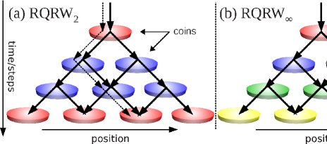
Figure 1: (color online) (a) The dashed line represents a possible realization of $CRW$, where no superposition occurs. The solid curves represent probability amplitudes for $RQRW_{2}$, where only two $C(t)$ are allowed (red and blue discs). (b) Schematic view for $RQRW_{\infty}$, where $C(t)$ are chosen randomly from uniform continuous distributions of quantum coins (at each step a different color/coin is used). Note that at each step all coins/colors are the same (dynamical disorder).

In the second RQRW we have an infinite number of $C(t)$ to choose at each step. The independent parameters of $C(t)$, namely, $q(t)$, $\theta(t)$, and $\varphi(t)$, are chosen from continuous uniform distributions spanning the range of their allowed values. Note that we can have a walk where either one, or two or all parameters change at each step. We call such walks $RQRW_{\infty}$.

Entanglement. Since $\rho(t)=|\Psi(t)\rangle\langle\Psi(t)|$ is pure we quantify the entanglement between the internal and external degrees of freedom by the von Neumann entropy of the partially reduced state $\rho_{C}(t)=Tr_{P}(\rho(t))$ ben96 , $S_{E}(\rho(t))=-Tr(\rho_{C}(t)\log_{2}\rho_{C}(t))$, with $Tr_{P}(\cdot)$ being the trace over the position degrees of freedom. $S_{E}$ is $0$ for separable states and $1$ for maximally entangled ones. Since $\rho_{C}(t)\!\!=\!\!\alpha(t)|\!\uparrow\rangle\langle\uparrow\!|\!+\!\beta(t)|\!\downarrow\rangle\langle\downarrow\!|\!+\!\gamma(t)$ $|\!\uparrow\rangle\langle\downarrow\!|\!+\!\gamma^{*}(t)|\!\downarrow\rangle\langle\uparrow\!|,$ where $\alpha(t)=\sum_{j}|a(j,t)|^{2},\beta(t)=\sum_{j}|b(j,t)|^{2},\gamma(t)=\sum_{j}a(j,t)b^{*}(j,t),$ and $z^{*}$ is the complex conjugate of $z$, we have $S_{E}(\rho(t))=-\lambda_{+}(t)log_{2}\lambda_{+}(t)-\lambda_{-}(t)log_{2}\lambda_{-}(t),$ with $\lambda_{\pm}=(1/2{\pm}\sqrt{1/4-\alpha(t)(1-\alpha(t))+|\gamma(t)|^{2}})$ being the eigenvalues of $\rho_{C}(t)$.

Results. We start studying two typical representatives of RQRW. The first one is $RQRW_{2}$ with $C_{1}$ being the Hadamard ($H$) coin ($q(t)=1/2$, $\theta(t)=\varphi(t)=0$) and $C_{2}$ the Fourier/Kempe ($F$) coin ($q(t)=1/2$, $\theta(t)=\varphi(t)=\pi/2$). Note that the latter coin introduces a $\pi/2$ relative phase between $|\!\uparrow\rangle$ and $|\!\downarrow\rangle$. The other walk is $RQRW_{\infty}$, where at each step the values of $q(t),\theta(t)$ and $\varphi(t)$ are chosen randomly from three distinct continuous uniform distributions.

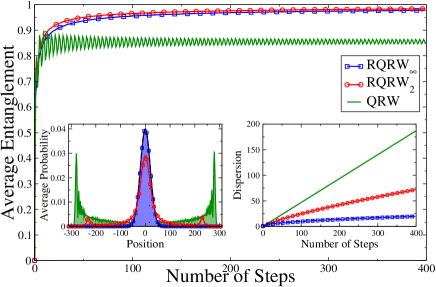
Figure 2: (color online) $\langle S_{E}\rangle$ was computed averaging over 16,384 initial conditions of the form, $|\Psi(0)\rangle=(\cos\alpha_{s}|\uparrow\rangle+e^{i\beta_{s}}\sin\alpha_{s}|\downarrow\rangle)\otimes(\cos\alpha_{p}|-1\rangle+e^{i\beta_{p}}\sin\alpha_{p}|1\rangle)$, with $\alpha_{s,p}\in[0,\pi]$ and $\beta_{s,p}\in[0,2\pi]$. The first realization used the initial condition $(\alpha_{s},\beta_{s},\alpha_{p},\beta_{p})=(0,0,0,0)$ and the subsequent ones all quadruples of points in independent increments of $0.4$ until $\alpha_{s,p}=\pi$ and $\beta_{s,p}=2\pi$. We worked with a $400$-step walk. The blue/square curve gives $RQRW_{\infty}$, the red/circle one $RQRW_{2}$, and the green/solid one the Hadamard $QRW$. The left inset shows the average position probability distributions ($\langle P(j)\rangle$) after $400$ steps and the right one the average dispersions ($\langle\sqrt{\sigma^{2}}\rangle$). The black/dashed curves represent the expected results for CRW starting at the origin, and they overlap with the curves for $RQRW_{\infty}$, which is more localized than $RQRW_{2}$. The two spikes on $\langle P(j)\rangle$ for $RQRW_{2}$ is due to the fact that it is built on the Hadamard and Fourier coins, where these spikes are a common trend.

In order to investigate the dependence of the asymptotic behavior of $S_{E}$ on initial conditions, we run several thousands numerical experiments, each of which with a different initial condition. Each realization of the walk gives at step $t$ a value for $S_{E}$ and in Fig. 2 we show the average values of $S_{E}$ over all realizations at each step $t$.

As can be seen from Fig. 2, the average entanglement $\langle S_{E}\rangle$ approaches the maximal value possible ($S_{E}=1$) for both RQRW cases after a few hundreds steps. For comparison, we show the usual QRW with a Hadamard coin, where clearly $\langle S_{E}\rangle\neq 1$ asymptotically. Indeed, for the ordered case the asymptotic value of $S_{E}$ is highly sensitive to the initial conditions and the set of initial states giving high values of $S_{E}$ is not dense. An important example is the Hadamard walk, where it can be shown car05 that the asymptotic values of $S_{E}$ continuously oscillate between $S_{E}=0.661$ and $S_{E}=0.979$ as we cover a set of initial conditions similar to the ones in Fig. 2.

To gain further insights into the asymptotic limit of $S_{E}$ we run another set of numerical experiments for the three walks described in Fig. 2, but now going up to 1000 steps and also counting the number of initial conditions leading to high values of $S_{E}$. Looking at Fig. 3 it is clear that $S_{E}\rightarrow 1$ for $RQRW_{\infty}$ and $RQRW_{2}$ while the Hadamard $QRW$ asymptotic entanglement is highly sensitive to the initial conditions.

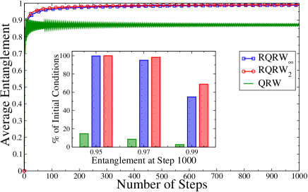
Figure 3: (color online) $\langle S_{E}\rangle$ was got averaging over 2,016 localized initial conditions given as $|\Psi(0)\rangle=(\cos\alpha_{s}|\uparrow\rangle+e^{i\beta_{s}}\sin\alpha_{s}|\downarrow\rangle)$ $\otimes|0\rangle$, where $\alpha_{s}\in[0,\pi]$ and $\beta_{s}\in[0,2\pi]$. The first realization used the initial condition $(\alpha_{s},\beta_{s})=(0,0)$ and the next ones all pairs of points in independent increments of $0.1$ until $\alpha_{s}=\pi$ and $\beta_{s}=2\pi$. We worked with a $1000$-step walk. The inset shows the rate of initial conditions leading to $S_{E}$ greater than $0.95$, $0.97$, and $0.99$ at step $1000$. Note that for RQRW (middle/blue and right/red bars) almost $100\%$ of the initial conditions lead to $S_{E}>0.97$ while for QRW (left/green bar) this occurs for less than $10\%$.

Now, since $S_{E}$ is bounded from above by one, $\langle S_{E}\rangle\rightarrow 1$ implies that for RQRW the set of initial states in which $S_{E}\rightarrow 1$ asymptotically is dense. In other words, this suggests that in the asymptotic limit $S_{E}\rightarrow 1$ for any initial condition. The justification of the last assertion is given by the following theorem.

Theorem. In the asymptotic limit and for any initial condition, $S_{E}\rightarrow 1$ if the quantum coin acting on the walker at each step is a random $SU(2)$ unitary operator.

Here we outline the main ideas leading to the proof and the details are given in Appendix B. In the long time regime $\rho_{C}(t+1)=\rho_{C}(t)+\mathcal{O}(t^{-1/4})$. Thus, $\rho_{C}(t+1)$ $=$ $\rho_{C}(t)$ for $t$ $\rightarrow$ $\infty$. In terms of its coefficients $\alpha(t+1)=\alpha(t)$ and $\gamma(t+1)=\gamma(t)$. This, plus the time evolution of $\alpha(t)$ and $\gamma(t)$, that can be computed with Eq. (2), leads to $\mathrm{Re}$ $[(c_{\uparrow\uparrow}(t+2)/c_{\uparrow\downarrow}(t+2)$ $-$ $c_{\uparrow\uparrow}(t+1)/c_{\uparrow\downarrow}(t+1))$ $\gamma(t)]$ $=$ $0$. Note that for constant coins, this equality is trivially satisfied. But for time dependent random ones, the term inside the parenthesis is a random complex number $z(t)=x(t)+iy(t)$, with $x(t)$ and $y(t)$ random reals. Hence $x(t)\mathrm{Re}[\gamma(t)]-y(t)\mathrm{Im}[\gamma(t)]=0.$ Repeating this argument for a subsequent time leads to $x(t+1)\mathrm{Re}[\gamma(t)]-y(t+1)\mathrm{Im}[\gamma(t)]=0.$ These expressions form a homogeneous system of linear equations on the variables $\mathrm{Re}[\gamma(t)]$ and $\mathrm{Im}[\gamma(t)]$. A non-trivial solution exists if the determinant of its coefficients is zero. But this will almost surely not happen since $x(t),y(t),x(t+1)$, and $y(t+1)$ are four independent random numbers. Thus $\gamma(t)=0$ and $\alpha(t)=1/2$, since the dynamics and the asymptotic condition give $\alpha(t)=1/2+\mathrm{Re}[\gamma(t)c_{\uparrow\uparrow}(t+1)/c_{\uparrow\downarrow}(t+1)]$. These values for $\gamma(t)$ and $\alpha(t)$ gives $S_{E}=1$, a maximally entangled state.

In Appendix C we investigate numerically other RQRW, some of them not covered by the theorem, and how much disorder we must have to achieve $S_{E}\rightarrow 1$ asymptotically. We show that weak disorder is sufficient to generate highly entangled states for arbitrary initial conditions in a variety of RQRW and give further details about the probability distribution of the walker and its dispersion properties. Finally, we also investigate how fast highly non-local initial conditions (Gaussian distributions) approach the asymptotic limit $S_{E}\rightarrow 1$.

Experimental implementation. Current technology allows one to implement in at least two ways the previous walks. The first one is based on passive optical elements, such as quarter (QWP) and half (HWP) wave plates and polarizing beam-splitters (PBS), plus a fast-switching electro-optical modulator (EOM) sch10 , where the internal degree of freedom of the walker is the polarization of a photon and the position/external one is mapped to different arrival times of the photon at the photodetector (time bins) experiment1 .

The second way also uses photons as walkers but it is based on integrated photonics, where a disordered walk is built on integrated waveguide circuits, providing perfect phase stability. By using state-of-the-art femtosecond laser writing techniques, the authors in cre13 were able to wrought an array of interferometers in a glass that reproduces the dynamics of RQRW experiment2 .

To test the ideas here presented we need to measure the entanglement of the walker, which is obtained if we know the coin state $\rho_{C}(t)$. But $\rho_{C}(t)$ is determined by slightly changing the two schemes outlined above. Indeed, since a general photon polarization state is written as $\rho_{C}(t)=\mathbb{1}_{C}+\sum_{j=1}^{3}r_{j}\sigma_{j}$, with $\sigma_{j}$ being Pauli matrices, we can determine $\rho_{C}(t)$ if we measure $r_{j}$. But this is achieved by measuring the average polarization of the photon in the vertical/horizontal axis ($r_{3}$), in the $\pm 45^{o}$ axis ($r_{1}$), and the average right/left circular polarization ($r_{2}$) per02 . These measurements can be easily implemented by properly arranging a HWP and QWP before the photon passes a PBS with photodetectors at each one of its arms. Note that the raw data are related to $\rho(t)$ and we need to trace out its position degrees of freedom (post-processing measurement) to get $\rho_{C}(t)$. In Appendix D we show that just a few steps are enough to have different predictions for the behavior of $S_{E}$ if we work with either $RQRW_{2}$ or QRW.

Summary. We defined the random quantum random walk (RQRW), a discrete time quantum random walk scheme whose unitary evolution at each step is chosen randomly using a two-sided (or infinitely-sided) classical coin. We showed that both the usual classical and quantum random walks are particular cases of RQRW. We then studied its entanglement generation capacity. We showed that RQRW creates maximally entangled sates in the asymptotic limit for several types of dynamical disorder (random time evolution), contrary to the ordered QRW. Furthermore, and surprisingly, we proved that RQRW entanglement creation capabilities are independent of the initial condition of the walker, another property in contrast to ordered QRW.

Finally, we would like to point out that our findings naturally lead to new important questions. For example, what is the interplay between order/disorder and entanglement creation for two- or three-dimensional walkers? What would happen to the entanglement for static disorder cha12 ; sch10 ; cre13 ? Can the previous results be adapted to the case of two or more bos09 walkers to improve the creation of bipartite and multipartite entanglement, respectively, only among the internal degrees of freedom? We believe investigations along these lines may bring other unexpected and intriguing results and foster the development of new entanglement generation protocols.

Appendix A Proof that QRW and CRW are particular cases of RQRW

Consider a one-dimensional lattice of regularly spaced points, where each point corresponds to the positions a classical particle can be found. Let us assume this particle moves right or left according to the result of a coin tossing game. The probability of obtaining heads (moves right) is $p$ and of getting tails (moves left) is $1-p$. This process is known as the one-dimensional discrete time classical random walk (CRW) and we call it unbiased or symmetric if we deal with a fair coin ($p=1/2$) and biased otherwise.

Looking at $C(t)$, Eq. (13), we see that it changes at each step by how $q(t)$, $\theta(t)$, and $\varphi(t)$ change with time. If they are constant in time we recover QRW. Moreover, assume the system’s initial state is $|\!\phi\rangle\otimes|0\rangle$, with $|\phi\rangle$ an arbitrary spin state and let the initial coin be such that $C(1)|\phi\rangle=|\!\uparrow\rangle$. This can always be achieved since $C(t)$ is an arbitrary $SU(2)$ rotation. Since $U(t)=S(C(t)\otimes\mathbb{1}_{P})$ we see that after the first step the particle moves right. Now, for $t\geq 2$ let $C(t)$ be chosen between two choices according to the result of a classical coin tossing in the following way. If one gets heads $C(t)$ is chosen such that the particle moves right and if one gets tails it is chosen such that the particle moves left. The first case is achieved by choosing $C(t)=\mathbb{1}_{C}$ ($\sigma_{1}$) if the spin state is $|\!\uparrow\rangle$ ($|\!\downarrow\rangle$) and the second one by choosing $C(t)=\sigma_{1}$ ($\mathbb{1}_{C}$) if the spin state is $|\!\uparrow\rangle$ ($|\!\downarrow\rangle$), where $\sigma_{1}$ is the spin flip operator ($q(t)=\theta(t)=\varphi(t)=0$). It is not difficult to see that this is an exact simulation of CRW and a proof that it is a particular case of RQRW.

Appendix B Proof of Theorem

B.1 The proof

We want to prove the following theorem:

Theorem. In the asymptotic limit and for any initial condition, $S_{E}\rightarrow 1$ if the quantum coin acting on the walker at each step is a random $SU(2)$ unitary operator.

Before we start, we must clarify what we mean by “the asymptotic limit”. First, the asymptotic limit is associated to the long time behavior of the reduced density matrix $\rho_{C}(t)=Tr_{P}(\rho(t))$ describing the internal degrees of freedom of the system. Here $\rho(t)=|\Psi(t)\rangle\langle\Psi(t)|$ and $|\Psi(t)\rangle$ $=$ $\sum_{j}(a(j,t)|\!\uparrow\rangle|j\rangle$ $+$ $b(j,t)|\!\downarrow\rangle|j\rangle)$. This asymptotic condition was analytically proved for QRW in the second reference of car05 and in Sec. B.2 we numerically show that this is also true for RQRW. More specifically, we show that in the long time regime $\rho_{C}(t+1)=\rho_{C}(t)+\mathcal{O}(t^{-1/4})$, where $\mathcal{O}(t^{-1/4})$ is at most of order $t^{-1/4}$. Therefore, when we invoke the asymptotic limit, it is implied that we are in the limit $t\rightarrow\infty$ and slightly abuse notation by writing $\rho_{C}(t+1)=\rho_{C}(t)$ from the start. Note that all steps in the proof could be carried out by using $\rho_{C}(t+1)=\rho_{C}(t)+\mathcal{O}(t^{-1/4})$ and taking the limit at the last step of the proof. This would introduce in all expressions below an $\mathcal{O}(t^{-1/4})$ term which would vanish when $t\rightarrow\infty$.

Let us start the proof by writing

$$\rho_{C}(t)=\left(\begin{array}[]{cc}\alpha(t)&\gamma(t)\\ \gamma^{*}(t)&\beta(t)\end{array}\right),$$

where $\alpha(t)=\sum_{j}|a(j,t)|^{2}$, $\beta(t)=\sum_{j}|b(j,t)|^{2}$, and $\gamma(t)=\sum_{j}a(j,t)b^{*}(j,t)$. With this notation, the asymptotic limit as discussed above implies $\alpha(t+1)=\alpha(t)$, $\beta(t+1)=\beta(t)$, and $\gamma(t+1)=\gamma(t)$.

For any initial condition, the time evolution of the system for a given RQRW is given by

$$a(j,t+1)\! \!=\! \!c_{\uparrow\uparrow}(t+1)a(j-1,t)+c_{\uparrow\downarrow}(t+1)b(j-1,t),$$

$$b(j,t+1)\! \!=\! \!c_{\downarrow\uparrow}(t+1)a(j+1,t)+c_{\downarrow\downarrow}(t+1)b(j+1,t),$$

where different RQRW’s are obtained changing the way $c_{jk}(t)$, $j,k=\uparrow,\downarrow$, evolves with time.

Using Eq. (LABEL:Arecurrence) we have

$$\alpha(t+1) = \sum_{j}a(j,t+1)a^{*}(j,t+1)$$ (4)

$$= |c_{\uparrow\uparrow}(t+1)|^{2}\alpha(t)+|c_{\uparrow\downarrow}(t+1)|^{2}\beta(t)$$

$$+2\mathrm{Re}[c_{\uparrow\uparrow}(t+1)c^{*}_{\uparrow\downarrow}(t+1)\gamma(t)],$$

where $\mathrm{Re}[z]$ is the real part of the number $z$. Now, employing the unitarity of the coin ($|c_{\uparrow\uparrow}(t+1)|^{2}+|c_{\uparrow\downarrow}(t+1)|^{2}$ $=$ $1$) and the normalization condition ($\alpha(t)+\beta(t)=1$) we have

$$\alpha(t+1) = |c_{\uparrow\downarrow}(t+1)|^{2}+(1-2|c_{\uparrow\downarrow}(t+1)|^{2})\alpha(t)$$ (5)

$$+2\mathrm{Re}[c_{\uparrow\uparrow}(t+1)c^{*}_{\uparrow\downarrow}(t+1)\gamma(t)].$$

Finally, using the assumption that we are in the asymptotic limit ($\alpha(t+1)=\alpha(t)$) we obtain

$$\alpha(t)=\frac{1}{2}+\mathrm{Re}\left[\frac{c_{\uparrow\uparrow}(t+1)}{c_{\uparrow\downarrow}(t+1)}\gamma(t)\right].$$ (6)

Similarly, starting with $\beta(t+1)$ in Eq. (4) we get

$$\beta(t)=\frac{1}{2}+\mathrm{Re}\left[\frac{c^{*}_{\downarrow\downarrow}(t+1)}{c^{*}_{\downarrow\uparrow}(t+1)}\gamma(t)\right].$$ (7)

Invoking again that we are in the asymptotic limit, $\alpha(t+1)=\alpha(t)$, we have after inserting Eq. (6) in the previous relation,

$$\mathrm{Re}\left[\left(\frac{c_{\uparrow\uparrow}(t+2)}{c_{\uparrow\downarrow}(t+2)}-\frac{c_{\uparrow\uparrow}(t+1)}{c_{\uparrow\downarrow}(t+1)}\right)\gamma(t)\right]=0,$$ (8)

where we have used that $\gamma(t+1)=\gamma(t)$ to arrive at the last equality. Since we are dealing with random $SU(2)$ unitary matrices, the term inside the parenthesis above is a random complex number $z(t)=x(t)+iy(t)$, with $x(t)$ and $y(t)$ random reals. Writing $\gamma(t)=\mathrm{Re}[\gamma(t)]+i\mathrm{Im}[\gamma(t)]$, Eq. (8) implies

$$x(t)\mathrm{Re}[\gamma(t)]-y(t)\mathrm{Im}[\gamma(t)]=0.$$ (9)

We can repeat the previous argument starting with $\alpha(t+2)=\alpha(t+1)$. Using the asymptotic assumption that $\gamma(t+2)=\gamma(t+1)=\gamma(t)$ leads to

$$x(t+1)\mathrm{Re}[\gamma(t)]-y(t+1)\mathrm{Im}[\gamma(t)]=0.$$ (10)

Now, Eqs. (9) and (10) constitute a homogeneous system of linear equations on the variables $\mathrm{Re}[\gamma(t)]$ and $\mathrm{Im}[\gamma(t)]$. We can only achieve a non-trivial solution if the determinant of its coefficients is zero, i.e., if $x(t)y(t+1)=y(t)x(t+1)$. But this will almost surely not happen since $x(t),y(t),x(t+1)$, and $y(t+1)$ are four independent random real numbers and we have $x(t)y(t+1)\neq y(t)x(t+1)$. Hence, Eqs. (9) and (10) imply

$$\mathrm{Re}[\gamma(t)]=\mathrm{Im}[\gamma(t)]=0\rightarrow\gamma(t)=0,$$ (11)

and consequently (see Eqs. (6) and (7))

$$\alpha(t)=\beta(t)=1/2.$$ (12)

Finally, inserting the asymptotic values of $\alpha(t)$, $\beta(t)$, and $\gamma(t)$ just computed into the expression for $\rho_{C}(t)$ we get

$$\rho_{C}(t)=\left(\begin{array}[]{cc}1/2&0\\ 0&1/2\end{array}\right),$$

which immediately leads to the maximal allowed value for the entanglement, $S_{E}=-Tr(\rho_{C}(t)\log_{2}\rho_{C}(t))=1.\square$

Remark 1: The previous proof also applies whenever we have a quantum coin $C(t)$ with at least $\theta(t)$ random; and also with only random $q(t)$ and with $\theta(t)$ not zero or a multiple of $\pi/2$. To see that, let us rewrite here the quantum coin,

$$C(t)=\left(\begin{array}[]{cc}c_{\uparrow\uparrow}(t)&c_{\uparrow\downarrow}(t)\\ c_{\downarrow\uparrow}(t)&c_{\downarrow\downarrow}(t)\end{array}\right),$$ (13)

with $c_{\uparrow\uparrow}(t)=\sqrt{q(t)}$, $c_{\uparrow\downarrow}(t)=\sqrt{1-q(t)}e^{i\theta(t)}$, $c_{\downarrow\uparrow}(t)=\sqrt{1-q(t)}e^{i\varphi(t)}$, and $c_{\downarrow\downarrow}(t)=-\sqrt{q(t)}e^{i(\theta(t)+\varphi(t))}$. Here $0\leq q(t)\leq 1$, $0\leq\theta(t)\leq 2\pi$, and $0\leq\varphi(t)\leq 2\pi$ footnote3 .

If we take the case where at least $\theta(t)$ changes randomly with time, with $\varphi(t)$ or $q(t)$ changing or not, we see that $c_{\uparrow\uparrow}(t)/c_{\uparrow\downarrow}(t)$ $=$ $\sqrt{q(t)/(1-q(t))}e^{-i\theta(t)}$ is a random complex number due to the randomness of $\theta(t)$. (Note that arguments based on the last equation is not valid whenever we have a fixed $q(t)=0$ or $q(t)=1$.) Therefore, Eq. (6) has the same properties as in the original proof and implies Eqs. (8), (9) and (10). The same argument holds for Eq. (7). In other words, the whole proof follows if we guarantee in Eq. (6) or in Eq. (7) that we have random complex numbers multiplying $\gamma(t)$ at each step. By this simple argument we have proved that in the asymptotic limit $S_{E}\rightarrow 1$ for four cases: all parameters randomly changing with time (the original proof), $\theta(t)$ and $\varphi(t)$ random with $q(t)$ fixed, $\theta(t)$ and $q(t)$ random with $\varphi(t)$ fixed, and $\theta(t)$ random with both $\varphi(t)$ and $q(t)$ fixed.

For $q(t)$ random and $\theta(t)$ fixed but not zero or a multiple of $\pi/2$ we have $c_{\uparrow\uparrow}(t)/c_{\uparrow\downarrow}(t)=\sqrt{q(t)/(1-q(t))}e^{-i\theta(t)}$, which due to the randomness of $q(t)$ is a random complex number and the proof follows. Note that if $\theta(t)=0$, $\theta(t)=\pi/2$, or $\theta(t)=\pi$, the proof cannot be carried out to its completion. In the first and third cases $c_{\uparrow\uparrow}(t)/c_{\uparrow\downarrow}(t)$ is a random real and following the steps of the proof leads only to $\mathrm{Re}[\gamma(t)]=0$; nothing can be said about the imaginary part of $\gamma(t)$. And in the second case $c_{\uparrow\uparrow}(t)/c_{\uparrow\downarrow}(t)$ is a random pure imaginary leading to $\mathrm{Im}[\gamma(t)]=0$, while nothing can be said about the real part.

Remark 2: The structure of the proof does not allow us to reach any conclusion when only $\varphi(t)$ changes. Noting that $c_{\uparrow\uparrow}(t)/c_{\uparrow\downarrow}(t)=\sqrt{q(t)/(1-q(t))}e^{-i\theta(t)}$ and $c_{\downarrow\downarrow}(t)/c_{\downarrow\uparrow}(t)=$ $-\sqrt{q(t)/(1-q(t))}e^{i\theta(t)}$, we see that they are both complex constants if only $\varphi(t)$ changes. Thus, since we do not have random complex numbers multiplying $\gamma(t)$ in either Eq. (6) or (7), the proof cannot follow.

Remark 3: Although the proof here cannot be extended to some particular cases that do not explore the full $SU(2)$ structure of the coin $C(t)$, numerical simulations (see the main text and Sec. C) suggest that if we have at least one of the three independent parameters of $C(t)$ random, we obtain $S_{E}\rightarrow 1$ asymptotically. Also, we found no analytical proof that the binary randomness of the balanced or unbalanced $RQRW_{2}$ leads to maximal entanglement asymptotically. However, extensive numerical analysis showed that this is true (see main text and Sec. C).

Remark 4: Finally, the proof does not tell us when the system will approach the asymptotic limit. It may happen for a few hundreds steps or we may need several thousands or more steps. As we show in Sec. C, the more delocalized in position the initial condition the more steps we need.

B.2 Numerical proof of the asymptotic assumption

The previous theorem has two assumptions that led to the proof of its thesis. The first one is related to the dynamical property of the walker we are dealing with: we have random $SU(2)$ unitary coins at each time step. Without this random feature, i.e., if we were dealing with a fixed coin, Eq. (8) is trivially satisfied and the proof does not follow. Indeed, for a fixed coin we have $c_{jk}(t)=c_{jk}(t+1)$, with $j,k=\uparrow,\downarrow$. This makes the term inside the parenthesis of Eq. (8) zero and nothing can be said about $\gamma(t)$.

The second ingredient is the asymptotic assumption, namely, $\lim_{t\rightarrow\infty}[\rho_{C}(t+1)-\rho_{C}(t)]=0$, a sufficient (but not necessary) condition for $S_{E}(\rho(t+1))=S_{E}(\rho(t))$. It is a sufficient condition for the asymptotic behavior of the entanglement since $S_{E}(\rho(t))$ is a function of the coefficients of $\rho_{C}(t)$ (see the main text).

For the Hadamard QRW it was analytically shown that the asymptotic assumption is a consequence of the dynamics of the walker (see second reference of car05 ). Our goal here is to provide a numerical proof that the same fact holds for RQRW. Moreover, we also investigate the rate at which the asymptotic limit is achieved for both QRW and RQRW. We find the interesting fact that the two rates obey a power law with different exponents.

In order to quantify the rate at which the asymptotic limit is approached we compute the trace distance nie2000 between two adjacent states in time,

$$D(t)=\frac{1}{2}\text{Tr}\left(\left|\rho_{C}(t)-\rho_{C}(t-1)\right|\right),$$ (14)

where $|A|=\sqrt{A^{\dagger}A}$. For a qubit it is not difficult to show that the trace distance $D(t)$ is equal to the Ky Fan 1-norm (largest singular value of $\rho_{C}(t)-\rho_{C}(t-1))$ and that the Frobenius norm of $\rho_{C}(t)-\rho_{C}(t-1)$ equals $\sqrt{2}D(t)$. In other words, the results we obtain in what follows are quite independent of the norm we choose to work with.

A direct computation gives

$$D(t)=\frac{1}{2}\sqrt{(\Delta r_{1}(t))^{2}+(\Delta r_{2}(t))^{2}+(\Delta r_{3}(t))^{2}},$$ (15)

where $\Delta r_{j}(t)=\text{Tr}(\rho_{C}(t)\sigma_{j})-\text{Tr}(\rho_{C}(t-1)\sigma_{j})$, with $\sigma_{j}$ being the Pauli matrices.

The first series of numerical experiments we implemented is shown in Fig. 4. We worked with the Hadamard QRW and $RQRW_{\infty}$ with random $q(t)$, $\theta(t)$, and $\varphi(t)$. We computed $D(t)$ for hundreds of random initial conditions and plotted the average trace distance. As can be seen from the fitted curves, both QRW and $RQRW_{\infty}$ approach the asymptotic limit ($\langle D(t)\rangle\rightarrow 0$) with a power law. For QRW a $95\%$ confidence level non-linear fitting gave $D(t)=(0.331217\pm 0.000006)t^{-1/2}$ and $D(t)=(0.4977\pm 0.0003)t^{-1/4}$ for $RQRW_{\infty}$.

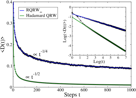
Figure 4: (color online) The curves were plotted averaging over 1000 random initial conditions of the following form, $|\Psi(0)\rangle=(\cos\alpha_{s}|\uparrow\rangle+e^{i\beta_{s}}\sin\alpha_{s}|\downarrow\rangle)\otimes(\cos\alpha_{p}|-1\rangle+e^{i\beta_{p}}\sin\alpha_{p}|1\rangle)$, where $\alpha_{s,p}\in[0,\pi]$ and $\beta_{s,p}\in[0,2\pi]$. We worked with a $1000$-step walk. The lower curve is the Hadamard QRW and the upper curve $RQRW_{\infty}$ with all its three parameters randomly chosen at each step from the following uniform distributions: $q(t)\in[0,1],\theta(t)\in[0,\pi]$, and $\varphi(t)\in[0,2\pi]$. The small circles are the simulated $\langle D(t)\rangle$ and the solid lines fitted curves to the data. The inset shows the log-log plot of the main graph. A $95\%$ confidence level linear fitting gives, as expected, $-0.2504\pm 0.0005$ for the slope of the $RQRW_{\infty}$ line and $-0.5102\pm 0.0007$ for the slope of the Hadamard QRW line. If we drop the initial points to implement the fitting and focus on the asymptotic ones, the slopes approach even more the respective values $-1/4$ and $-1/2$.

We have also studied the behavior of $\langle D(t)\rangle$ for the other $RQRW_{\infty}$ and for $RQRW_{2}$. As can be seen in Fig. 5, for all cases $D(t)\sim t^{-1/4}$.

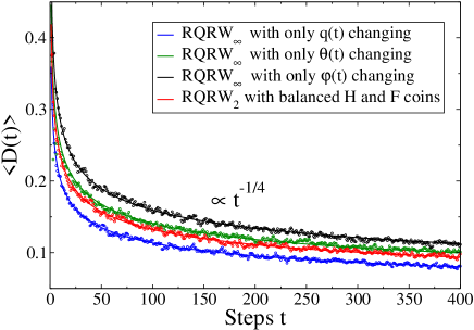
Figure 5: (color online) The curves were plotted averaging over 500 random initial conditions as given in Fig. 4. We worked with a $400$-step walk. The small circles are the simulated $\langle D(t)\rangle$ and the solid lines fitted curves to the data. We assumed that $q(t)\in[0,1],\theta(t)\in[0,\pi]$, and $\varphi(t)\in[0,2\pi]$.

Finally, we have extended the previous analysis to the matrix coefficients of $\rho_{C}(t)$, i.e., we have computed $\langle|\alpha(t)-\alpha(t-1)|\rangle$, $\langle|\mathrm{Re}[\gamma(t)]-\mathrm{Re}[\gamma(t-1)]|\rangle$, and $\langle|\mathrm{Im}[\gamma(t)]-\mathrm{Im}[\gamma(t-1)]|\rangle$ for several hundreds steps and initial conditions. For the Hadamard QRW the dominant quantities go to zero as $t^{-1/2}$ and for all RQRW as $t^{-1/4}$. These and the previous results are clear numerical indications that $\rho_{C}(t)$ has an asymptotic limit whose origin can be traced to the dynamics of those quantum random walks and that this limit is approached differently whether we have an ordered or disordered walk.

B.3 The importance of being random in time

One may ask whether the origin of the maximal entanglement generation capability of RQRW is in the randomness of the coin or in the fact that it is time dependent. As we show below, its origin can be traced back to both ingredients occurring at the same time.

First, one calculation in Ref. cha12 shows that static disorder may decrease the effectiveness of a quantum walk to generate entanglement, far below the entanglement generation capacity of the ordered case. In other words, the presence of random coins at each position/site of the walk, and fixed throughout the whole evolution (static disorder), does not help in the generation of entanglement. However, care should be taken in generalizing this interpretation since in cha12 only one initial condition for a particular type of static disorder was numerically investigated, and for just a 100-step walk.

Second, what about the time-dependence alone? That is, what will be the behavior of the entanglement generation capacity of QRW if non-random time dependent coins are employed? In what follows we investigate this matter for periodic time dependent coins.

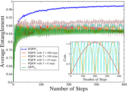
Figure 6: (color online) The curves were plotted averaging over 500 random initial conditions as given in Fig. 4. We worked with a $400$-step walk. The blue/square curve represents $RQRW_{\infty}$ with $q(t)=1/2$ and $\theta(t)=\varphi(t)$ randomly chosen from a uniform distribution ranging from $0$ to $2\pi$. The green curve represents the ordered QRW with the Hadamard coin. The other curves are PQRW’s evolving according to Eq. (16). The inset shows how the coin ($\theta(t)$) changes during the whole evolution for the PQRW’s with $T=400,100$, and $25$ steps.

In Fig. 6 we work with QRW’s such that the coin oscillates smoothly (in a time-discretized sense) between the Hadamard and Fourier coins. Therefore, for these coins $q(t)=1/2$ and $\varphi(t)=\theta(t)$, with

$$\theta(t)=\frac{\pi}{2}\left|\sin(\pi t/T)\right|.$$ (16)

Here $T$ is the period of oscillation and $t$ denotes the time-steps. We call these walks periodic quantum random walks (PQRW).

As can be seen from Fig. 6, only $RQRW_{\infty}$ approaches unity entanglement asymptotically. Also, the average entanglement for all PQRW oscillates with increasing amplitude as we decrease the period $T$. We can also note that the oscillation of the average entanglement of the ordered case diminishes much faster than those for PQRW. Actually, for small $T$, the amplitude of oscillation for the average entanglement decreases and then increases again with time for PQRW. This suggests that an asymptotic limit may not be achieved for such time-dependent coins. Or, if it occurs, it will happen at very long times when compared to the ordered case (see the brown/$T=8$ curve in Fig. 6 and also Fig. 7).

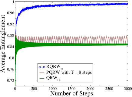
Figure 7: (color online) The curves were plotted averaging over 200 random initial conditions as given in Fig. 4. We worked with a $3000$-step walk. The blue/square curve represents the $RQRW_{\infty}$ as described in Fig. 6, the middle/brown curve $PQRW$ with $T=8$ steps and coin evolving according to Eq. (16), and the lower/green curve represents the ordered QRW with the Hadamard coin.

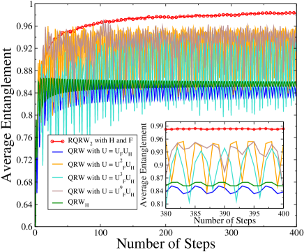
Figure 8: (color online) The curves were plotted averaging over 500 random initial conditions as given in Fig. 4. We worked with a $400$-step walk. The red/circle curve represents $RQRW_{2}$ with the Hadamard and Fourier coins. The green curve represents the ordered QRW with the Hadamard coin. The other curves are PQRW’s evolving according to Eq. (17). The inset shows the long time behavior of the curves given in the main graph.

We have also investigated a less smooth time dependence, such that one oscillates directly between the Hadamard and the Fourier coins. Noting that at each time-step the unitary evolution acting on the walker is $U(t)=S(C(t)\otimes\mathbb{1}_{P})$, we choose to work with the following time-dependent process

$$|\Psi(t+T)\rangle = U_{F}(t+T)\cdots U_{F}(t+2)U_{H}(t+1)|\Psi(t)\rangle$$ (17)

$$= U_{F}^{T-1}U_{H}|\Psi(t)\rangle,$$

where $U_{H}(t)=U_{H}=S(H\otimes\mathbb{1}_{P})$ and $U_{F}(t)=U_{F}=S(F\otimes\mathbb{1}_{P})$. Here $H$ and $F$ are the matrices representing, respectively, the Hadamard and Fourier coins and $T$ is the period, after which the whole sequence of unitaries repeats itself.

In Fig. 8 we show the behavior of the average entanglement for several periods $T$. We note that the average entanglement oscillates with greater amplitudes as compared to the smooth case. And as before, only the average entanglement for $RQRW_{2}$ clearly approaches the maximal value possible as we increase the number of steps.

Although more systematic studies are needed along these lines, in particular for static disorder, the results here presented suggest that neither time independent (static) disorder nor non-random time dependent coins are sufficient to generate maximally entangled states for any initial condition. Rather, random time dependent coins (dynamic disorder) appears to be essential to achieve such a feat.

Appendix C More numerical results

C.1 Several random initial conditions

Here we give more details about other RQRW’s. In addition to the average entanglement $\langle S_{E}\rangle$ we show the rate at which highly entangled states are generated, the average probability distribution for finding the qubit at a given position, and the dispersion for these RQRW’s.

The first thing worth mentioning is the robustness of these RQRW’s to generate highly entangled states, even if we have random coins very close to the Hadamard coin, i.e, even for not too big deviations from the values of $q(t)=1/2$ and $\theta(t)=\varphi(t)=0$ that characterize the H coin. Also, $RQRW_{\infty}$ with only $q(t)$ random (panel (b) of Fig. 9) has higher generation rates of highly entangled states than the other two $RQRW_{\infty}$, with either only $\theta(t)$ or $\varphi(t)$ changing (see panels (b) of Figs. 10 and 11). And if we look at Fig. 12.b, we see that $RQRW_{2}$ with H and F coins is the most efficient entanglement generator. It can produce highly entangled states for almost any initial condition within just a few hundreds steps, even for a very tiny deviation from the Fourier QRW ($p=0.05$).

We also note that the average probability distribution $\langle P(j)\rangle$ and the dispersion possess a wide range of behaviors. However, there is a common trend for all RQRW’s: the more we deviate from a fixed coin, the more it approaches the classical case. Also, among all $RQRW_{\infty}$ cases, the one in Fig. 9 gives the smallest peaks far from the origin (Fig. 9.c) while the other two cases exhibit the greatest symmetric peaks away from it. Furthermore, the weaker the disorder the greater the peaks. This is expected since for weaker disorder we are approaching the fixed coin case, where these peaks are a common trend.

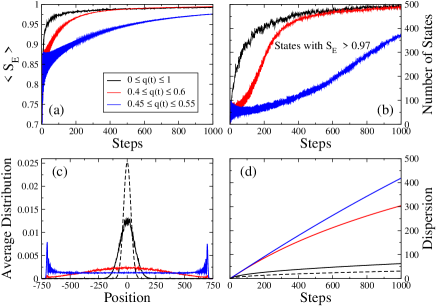
Figure 9: (color online) The following graphs were plotted averaging over 500 random initial conditions of the following form, $|\Psi(0)\rangle=(\cos\alpha_{s}|\uparrow\rangle+e^{i\beta_{s}}\sin\alpha_{s}|\downarrow\rangle)\otimes(\cos\alpha_{p}|-1\rangle+e^{i\beta_{p}}\sin\alpha_{p}|1\rangle)$, where $\alpha_{s,p}\in[0,\pi]$ and $\beta_{s,p}\in[0,2\pi]$. We worked with a $1000$-step walk and with $RQRW_{\infty}$ where $\theta(t)=\varphi(t)=0$ and at each step $q(t)$ was picked randomly from the three different uniform distributions given in (a), where the average entanglement $\langle S_{E}\rangle$ is shown for each case. The other graphs are: (b) The number of states with $S_{E}>0.97$ as a function of the discrete time steps. (c) The average probability distribution $\langle P(j)\rangle$ after $1000$ steps, with the dashed line showing the classical case. (d) The average dispersion $\langle\sqrt{\sigma^{2}}\rangle$ at each step, with the dashed line showing the classical dispersion curve. The classical case corresponds to a balanced CRW starting at the origin.

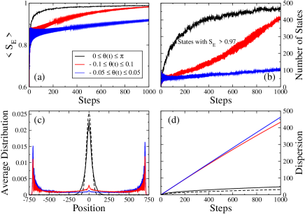
Figure 10: (color online) The following graphs were plotted averaging over 500 random initial conditions as given in Fig. 9 for a $1000$-step walk. Here $RQRW_{\infty}$ was such that $q(t)=1/2$, $\varphi(t)=0$ and at each step $\theta(t)$ was randomly chosen from the three different uniform distributions given in panel (a), where the average entanglement $\langle S_{E}\rangle$ is shown for each case. In panels (b), (c), and (d) we have the same as explained in Fig. 9.

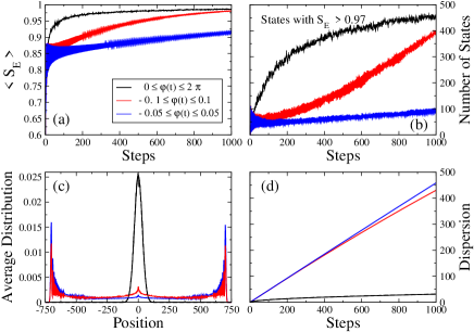
Figure 11: (color online) The following graphs were plotted averaging over 500 random initial conditions as given in Fig. 9 for a $1000$-step walk. Here $RQRW_{\infty}$ was such that $q(t)=1/2$, $\theta(t)=0$ and at each step $\varphi(t)$ was randomly chosen from the three different uniform distributions given in panel (a), where the average entanglement $\langle S_{E}\rangle$ is shown for each case. In panels (b), (c), and (d) we have the same quantities as given in Fig. 9. Note that here the classical case (dashed curves) overlap the solid/black ones.

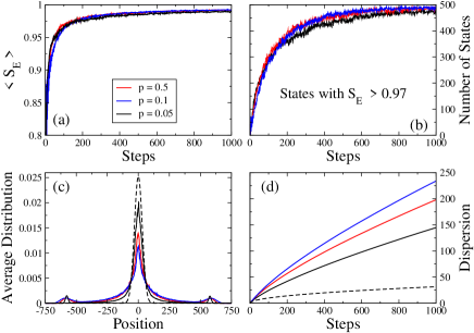
Figure 12: (color online) The following graphs were plotted averaging over 500 random initial conditions as given in Fig. 9 for a $1000$-step walk. Here we implement $RQRW_{2}$ with $p$ being the probability of using at step $t$ the Hadamard coin and $(1-p)$ the Fourier coin. In panel (a) we see the average entanglement $\langle S_{E}\rangle$ for each value of $p$. The other panels show the same quantities as explained in Fig. 9. Note that weak disorder is enough to guarantee $S_{E}\rightarrow 1$ asymptotically and it is remarkable that a mild deviation ($p=0.05$) from the Fourier/Kempe $QRW$ leads all initial conditions to almost perfectly entangled states after $1000$ steps. This illustrate the efficiency of this process to generate highly entangled states, even when weak disorder is present ($p=0.05$).

C.2 Delocalized Gaussian initial conditions

We now study the ability of RQRW’s against the standard QRW to entangle the external and internal degrees of freedoms of the walker for highly non-local/delocalized initial conditions in position. We will work with $RQRW_{\infty}$, with $q(t)$, $\theta(t)$, and $\varphi(t)$ completely random, and the Hadamard QRW.

The several initial positions of the qubit are given by Gaussian distributions centered about the origin,

$$\psi^{2}(x)=\frac{1}{\sqrt{2\pi\sigma^{2}}}e^{\frac{-x^{2}}{2\sigma^{2}}},$$

where $\sigma^{2}$ is the variance. The global initial state is therefore,

$$|\Psi(0)\rangle=|\xi\rangle\otimes\sum_{j=-\infty}^{\infty}\psi(j)|j\rangle,$$

where $\psi(j)\geq 0$ and we work with the discretized and normalized version of the Gaussian distribution. In what follows we will be working with two types of initial spin states, $|\xi_{1}\rangle=(|\uparrow\rangle$ $+i|\downarrow\rangle)/\sqrt{2}$ and $|\xi_{2}\rangle=(|\uparrow\rangle+|\downarrow\rangle)/\sqrt{2}$, and several Gaussians with dispersions ($\sigma$) as given in Fig. 13.

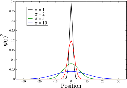
Figure 13: (color online) The wider the Gaussian curve the greater $\sigma$.

In Fig. 14 we plot the entanglement for both walks starting with the previous initial conditions. It is clear that the asymptotic entanglement of the Hadamard QRW is highly sensitive to initial conditions and many do not lead to maximal entanglement. For $RQRW_{\infty}$, we see the independence on the initial state for the asymptotic value of entanglement, although the rate at which it is approached depends on the broadness of the initial probability distribution for the position of the particle. Indeed, as we show in Fig. 15, for $\sigma=10$ the walker needs to travel about $6000$ steps to achieve $\langle S_{E}\rangle>0.9$. For just $1500$ steps, we have $\langle S_{E}\rangle\approx 0.8$.

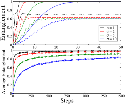
Figure 14: (color online) Upper panel: The solid curves represent the entanglement for Gaussian initial conditions with spin state $|\xi_{1}\rangle$ and the dashed ones with $|\xi_{2}\rangle$. We are working with the Hadamard QRW. Note that the asymptotic entanglement is extremely sensitive to initial conditions, where we can see it approaching a wide range of possible values. Lower panel: The same initial conditions as above but now we work with $RQRW_{\infty}$ where $q(t)\in[0,1],\theta(t)\in[0,\pi]$, and $\varphi(t)\in[0,2\pi]$. The solid and dashed curves are almost the same, so we employ up triangles to the cases starting with $|\xi_{1}\rangle$ and down triangles to those starting with $|\xi_{2}\rangle$. We now see that all cases approach the maximal entanglement value ($S_{E}\rightarrow 1$), although the greater the initial dispersion $\sigma$ the slower the rate at each the maximal value is approached. For $RQRW_{\infty}$ we implemented $500$ different realizations and plotted the average entanglement.

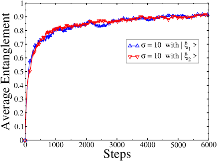
Figure 15: (color online) We implement $100$ realizations of $RQRW_{\infty}$ with $q(t)\in[0,1],\theta(t)\in[0,\pi]$, and $\varphi(t)\in[0,2\pi]$. We go up to $6000$ steps. Up triangles refer to $\langle S_{E}\rangle$ for the cases starting with $|\xi_{1}\rangle$ and down triangles to $|\xi_{2}\rangle$. Now we obtain $\langle S_{E}\rangle>0.9$ for a Gaussian with $\sigma=10$.

Finally, in Figs. 16 and 17 we show the probability distribution after $1500$ steps for walkers starting with the initial conditions given in Fig. 13 for the Hadamard QRW and $RQRW_{\infty}$, respectively.

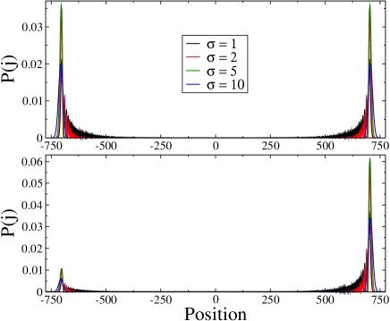
Figure 16: (color online) The upper panel shows the probability distributions $P(j)$ after $1500$ steps for initial conditions given by Gaussians with dispersion $\sigma$ and initial spin state $|\xi_{1}\rangle$ while the lower panel shows the cases with spin state $|\xi_{2}\rangle$. In both cases we have the Hadamard QRW. Note that $|\xi_{1}\rangle$ produces symmetrical peaks while $|\xi_{2}\rangle$ asymmetrical ones. The wider the initial conditions the wider the peaks.

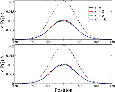
Figure 17: (color online) The upper panel shows the average probability distributions $\langle P(j)\rangle$ over $500$ realizations after $1500$ steps for initial conditions given by Gaussians with dispersion $\sigma$ and initial spin state $|\xi_{1}\rangle$. The lower panel shows the cases with spin state $|\xi_{2}\rangle$. In both cases we have $RQRW_{\infty}$ where $q(t)\in[0,1],\theta(t)\in[0,\pi]$, and $\varphi(t)\in[0,2\pi]$. Now all spin initial conditions give similar centralized peaks. The dashed line shows the expected classical $P(j)$ for a balanced CRW starting at the origin.

Appendix D Experimental predictions

The two experiments sch10 ; cre13 on which our experimental proposal is built achieve so far a few tens of steps. In particular, in sch10 RQRW’s with 28 steps were implemented. Our goal here is, therefore, to show that with just tens of steps we already have different predictions for the entanglement $S_{E}$ whether we implement the standard QRW or RQRW.

To build our experimental proposal, we started with the localized initial condition $|\Psi(0)\rangle=(\cos\alpha_{s}|\uparrow\rangle+e^{i\beta_{s}}\sin\alpha_{s}|\downarrow\rangle)$ $\otimes|0\rangle$ and searched in increments of $0.1$ for the pair of points $(\alpha_{s},\beta_{s})$ giving the lowest $S_{E}$ for the Hadamard QRW at step $28$. We found $(\alpha_{s},\beta_{s})=(2.7,\pi)$ with $S_{E}=0.645$. By keeping $\alpha_{s}=2.7$ and changing $\beta_{s}$ we get several different values for $S_{E}$ at step $28$ for the Hadamard QRW: $(\alpha_{s},\beta_{s})=(2.7,\pm\pi)\rightarrow S_{E}=0.645$, $(\alpha_{s},\beta_{s})=(2.7,0)\rightarrow S_{E}=0.983$, and $(\alpha_{s},\beta_{s})=(2.7,\pm\pi/2)\rightarrow S_{E}=0.869$. All these initial conditions can be easily prepared with half (HWP) and quarter wave plates (QWP).

Then, with the initial condition giving the lowest $S_{E}$ for the Hadamard QRW, we implemented $10,000$ numerical experiments using the balanced $RQRW_{2}$ with the Hadamard (H) and Fourier/Kempe (F) coins, searching for the sequence of random H’s and F’s giving the greatest entanglement. Using this sequence, we computed the entanglement for all initial conditions above: $(\alpha_{s},\beta_{s})=(2.7,\pm\pi)\rightarrow S_{E}=0.999$, $(\alpha_{s},\beta_{s})=(2.7,0)\rightarrow S_{E}=0.979$, $(\alpha_{s},\beta_{s})=(2.7,\pi/2)\rightarrow S_{E}=0.938$, and $(\alpha_{s},\beta_{s})=(2.7,-\pi/2)\rightarrow S_{E}=0.982$. As can be seen, with the $RQRW_{2}$ we already have after $28$ steps all these five initial conditions giving $S_{E}>0.93$, with four of them giving $S_{E}>0.97$. In contrast, the Hadamard QRW has only one initial condition giving $S_{E}>0.93$ and two of them giving $S_{E}<0.65$. This huge contrast can be experimentally detected with current day technology.

The sequence of H’s and F’s leading to such predictions is (with time flowing from left to right),

$$HHFHFFHFHFFHFHFHFFHFFHHFHFHH,$$

and it can be implemented in sch10 by adjusting the phase-shifter before the passage of the photon to the HWP that generates the standard coin and in cre13 by writing the integrated waveguide circuit with the correct optical path differences between successive directional couplers (the equivalent of polarizing beam splitters).

In Fig. 18 we show the entanglement time evolution for both the Hadamard $QRW$ and $RQRW_{2}$ for all the previous five initial conditions.

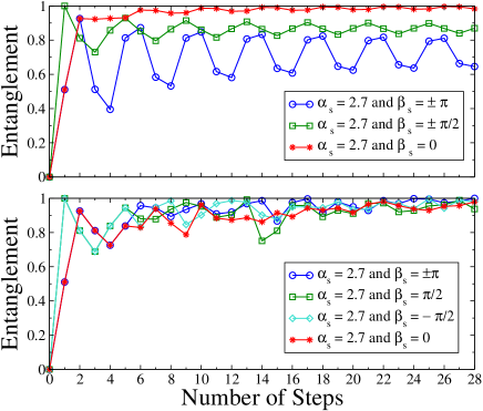
Figure 18: (color online) In the top panel we have the entanglement evolution for the Hadamard QRW and in the bottom panel its evolution for the $RQRW_{2}$ with a sequence of H and F coins as given in the text. Note that the entanglement at step $28$ for all initial conditions clusters around $0.9$ for $RQRW_{2}$ while it appreciably differs for different initial conditions for the Hadamard QRW. Also, note that for QRW the entanglement evolves oscillating periodically about its asymptotic value. For $RQRW_{2}$ this periodicity is lost.

The same analysis can be carried out to other RQRW’s in order to find a sequence of random coins that clearly gives different predictions for RQRW and QRW within just a few steps. In the asymptotic limit, of course, any random sequence will do.

References

- (1) This internal degree of freedom can be the spin of an electron, the polarization of photons or the ground and excited states of an atom.
- (2) Y. Aharonov, L. Davidovich, and N. Zagury, Phys. Rev. A 48, 1687 (1993).
- (3) J. Kempe, Contemp. Phys. 44, 307 (2003); S. E. Venegas-Andraca, Quantum Inf. Process. 11, 1015 (2012).
- (4) K. Pearson, Nature (London) 72, 294; 342 (1905); L. Rayleigh, ibid. 72, 318 (1905).
- (5) CRW is employed from the modeling of biological processes ber93 to polymer physics gen79 . QRW has proved to give important insights into the implementation of quantum search algorithms she03 , the understanding of the physics of photosynthesis eng07 , the construction of a universal quantum computer chi09 ; lov10 , and the generation of entangled states for systems with one car05 and more walkers bos09 .
- (6) H. C. Berg, Random Walks in Biology (Princeton University Press, New Jersey, 1993).
- (7) P.-G. de Gennes, Scaling Concepts in Polymer Physics (Cornell University Press, Ithaca, New York, 1979).
- (8) N. Shenvi, J. Kempe, and K. B. Whaley, Physical Review A 67, 052307 (2003).
- (9) G. S. Engel et al., Nature (London) 446, 782 (2007).
- (10) A. M. Childs, Phys. Rev. Lett. 102, 180501 (2009).
- (11) N. B. Lovett et al., Phys. Rev. A 81, 042330 (2010).
- (12) I. Carneiro et al., New J. Phys. 7, 156 (2005); G. Abal et al., Phys. Rev. A 73, 042302 (2006); S. Salimi and R. Yosefjani, Int. J. Mod. Phys. B 26, 1250112 (2012).
- (13) S. E. Venegas-Andraca and S. Bose, eprint arxiv: 0901.3946 [quant-ph]; S. K. Goyal and C. M. Chandrashekar, J. Phys. A: Math. Theor. 43, 235303 (2010); C. Di Franco, M. Mc Gettrick, and Th. Busch, Phys. Rev. Lett. 106, 080502 (2011); B. Allés, S. Gündüç, and Y. Gündüç, Quantum Inf. Process. 11, 211 (2012); E. Roldán et al., Phys. Rev. A 87, 022336 (2013); S. Moulieras, M. Lewenstein, and G. Puentes, eprint arXiv: 1211.1591 [quant-ph].
- (14) P. Ribeiro, P. Milman, and R. Mosseri, Phys. Rev. Lett. 93, 190503 (2004); M. C. Bañuls et al., Phys. Rev. A 73, 062304 (2006).
- (15) C. M. Chandrashekar, eprint arXiv:1212.5984 [quant-ph].
- (16) O. Buerschaper and K. Burnett, eprint arxiv: quant-ph/0406039; A. Wojcik et al., Phys. Rev. Lett. 93, 180601 (2004); A. Romanelli et al., Physica A 352, 409 (2005).
- (17) D. Shapira et al., Phys. Rev. A 68, 062315 (2003); A. Joye, Commun. Math. Phys. 307, 65 (2011).
- (18) A. Ahlbrecht et al., Quantum Inf. Process. 11, 1219 (2012); A. Ahlbrecht et al., J. Math. Phys. 52, 042201 (2011); A. Ahlbrecht, V. B. Scholz, and A. H. Werner, J. Math. Phys. 52, 102201 (2011).
- (19) C. H. Bennett et al., Phys. Rev. A 53, 2046 (1996).
- (20) A. Schreiber et al., Phys. Rev. Lett. 106, 180403 (2011); A. Schreiber et al., ibid. 104, 050502 (2010).
- (21) The random coin operator is implemented using HWP and EOM while the conditional displacement operator two PBS’s and a fiber delay line where one polarization follows a longer optical path. Also, arbitrary initial conditions are simply generated by QWP and HWP. An important feature of the scheme in sch10 is its scalability with the number of steps. Indeed, the techniques of optical feedback loop allow the implementation of a many-step walk using few optical elements. In sch10 the authors have already implemented -step walks with static and dynamical disorder.
- (22) A. Crespi et al., Nature Photon. 7, 322 (2013).
- (23) In integrated waveguide circuits PBS is a directional coupler and phase shifts are implemented writing circuits with different length/deformation.
- (24) A. Peres, Quantum Theory: Concepts and Methods (Kluwer Academic Publishers, New York, 2002).
- (25) The numerical results for the long time behavior in what follows are unchanged if we assume for example and . Also, the analytical proof of the theorem does not rely on specific choices for the ranges of and .
- (26) M. A. Nielsen and I. L. Chuang, Quantum Computation and Quantum Information (Cambridge University Press, Cambridge, 2000).