Deformation method for generalized Abelian Higgs-Chern-Simons models

Abstract

We present an extension of the deformation method applied to self-dual solutions of generalized Abelian Higgs-Chern-Simons models. Starting from a model defined by a potential $V(|\phi|)$ and a non-canonical kinetic term $\omega(|\phi|)|D_{\mu}\phi|^{2}$ whose analytical domain wall solutions are known, we show that this method allows to obtain an uncountable number of new analytical solutions of new models defined by other functions $\widetilde{V}$ and $\widetilde{\omega}$. We present some examples of deformation functions leading to new families of models and their associated analytic solutions.

1 Introduction

Topological defects play important role in several important areas such as high energy physics [1], cosmology [2] and condensed matter physics [3]. Such defects emerge as classical solutions of nonlinear field theories which possess degenerated vacua. Typical examples are domain walls described by kink solutions of the $\phi^{4}$ model, Ginzburg-Landau vortices and monopoles.

Usually, domain walls are solutions connecting two distinct vacua of scalar field theories in one-space dimension, or in their insertions in higher dimensions, while vortices emerge as solutions of models that couple charged matter fields with gauge fields living in a (at least) 3-dimensional space-time, and monopoles lie in a 4-D space-time.

In a (2+1)-dimensional space-time, minimal coupling between charged-matter and gauge fields can be implemented by the Chern-Simons (CS) action. Although the CS field can not be conceived as a free field, its coupling with matter fields imposes constraints in the dynamics which have very relevant consequences, in both, classical and quantum theories, with either relativistic or non-relativistic kinetics. In the non-relativistic (NR) framework, particles coupled through the CS field carry both electric charge and magnetic flux, and possess fractional statistics [4]. Additionally, the NR scalar CS model constitutes a seminal example of a Galilean-invariant gauge-field theory [5]. Also, for a critical strength of a quartic self-interaction of the scalar field, which restores the scale invariance [6], this model provides a field-theoretical description of the Aharonov-Bohm (AB) scattering [7]; considering the Lorentz covariant field theory, relativistic corrections to the AB scattering are obtained [8].

Self-dual soliton solutions have been found in the relativistic, ${\rm U}(1)$-invariant, Abelian, Higgs-Chern-Simons (HCS) gauge-theory where the symmetry-breaking potential of the Higgs field is $U(\varphi)\sim|\varphi|^{2}(|\varphi|^{2}-v^{2})^{2}$ [9]; vortex and domain-wall solutions have been obtained for this model [10]. This model was generalized by considering a non-canonical kinetic term for the complex scalar field, ${\cal W}(|\varphi|)|D_{\mu}\varphi|^{2}$, providing self-dual vortex [11] and domain-wall [12] solutions. Models with noncanonical kinetic terms (k-fields) find also applications in strong-interaction physics [13] and in cosmology [14].

Due to the nonlinearity, there is no general integration method to solve analytically the equations of motion of non-linear field theories; only for a small set of models, solutions of the equations of motion can be directly determined. However, for scalar fields in (1+1)-dimensions, starting from a nonlinear model with known solutions, infinitely many new models and their corresponding static solutions can be found using the deformation method [15]. This method works as follows. Choosing a deformation function $f(\phi)$, the model defined by the deformed potential $\widetilde{V}(\phi)=V[(f(\phi))]/[f^{\prime}(\phi)]^{2}$, where $f^{\prime}$ means the derivative of $f$, possesses static solutions given by $\widetilde{\phi}(x)=f^{-1}(\phi(x))$, where $\phi(x)$ is a solution of the static equation of motion of the original model with potential $V(\phi)$. This procedure has been applied to generate defect solutions of many models having polynomial interactions [16] and new families of sine-Gordon and multi-sine-Gordon models [17]. Also, an orbit-based extension of this method has been applied to models involving two interacting scalar fields [18].

The purpose of this Letter is to extend the deformation method to gauge-field models considering specifically the Abelian HCS theory, focusing particularly on the Jackiw-Lee-Weinberg (JLK) domain-wall solution [10]. In Section II, we present the generalized Abelian HCS models and write down the first-order equations obeyed by the Bogomol’nyi-Prasad-Sommerfeld (BPS) [19] domain-wall solutions. In Section III, the deformation method is extended to domain-wall solutions of generalized Abelian HCS models and some examples are given, illustrating the power of the procedure in generating new models with their static solutions. Finally, some remarks are made.

2 BPS domain walls in the generalized Abelian HCS model

We consider the generalized $(2+1)$-dimensional Abelian HCS model defined by the Lagrangian density [11]

$${\cal L_{S}}={\cal W}(|\varphi|)|D_{\mu}\varphi|^{2}-U(|\varphi|)+\frac{\kappa}{4}\epsilon^{\alpha\beta\gamma}{\cal A}_{\alpha}{\cal F}_{\beta\gamma},$$ (1)

where $\varphi$ is the complex Higgs field, $D_{\mu}=\partial_{\mu}+ie{\cal A}_{\mu}$ is the covariant derivative and ${\cal F}_{\mu\nu}=\partial_{\mu}{\cal A}_{\nu}-\partial_{\nu}{\cal A}_{\mu}$ is the field strength tensor of the gauge potential ${\cal A}_{\mu}$. The self-interaction potential, $U(|\varphi|)$, is assumed to implement a symmetry-breaking mechanism and the non-canonicity of the kinetic term is engendered by the function ${\cal W}(|\varphi|)$; taking ${\cal W}\equiv 1$, one recovers the standard Abelian HCS model. Note that, in the CS term, $\epsilon^{\alpha\beta\gamma}$ is the fully antisymmetric tensor and the electric and the magnetic CS fields are ${\cal E}^{i}={\cal F}^{i0}=-{\dot{\cal A}}^{i}-\nabla_{i}{\cal A}^{0}$ and ${{\cal B}}=\vec{\nabla}\times\vec{{\cal A}}=\partial_{2}{\cal A}_{1}-\partial_{1}{\cal A}_{2}$, respectively.

It is convenient to work with dimensionless quantities. In $(2+1)$ dimensions, the scalar field $\varphi$ has mass dimension equal to $1/2$, the same one we take for the gauge field; this choice ensures that the mass dimension of ${\cal A}_{\alpha}$ agrees with the one obtained if a Maxwell term were added to ${\cal L_{S}}$. It follows that the electric charge $e$ and the CS parameter $\kappa$ has mass dimensions equal to $1/2$ and $1$, respectively, so that $e^{2}/\kappa$ is dimensionless. We can get an additional simplification if we absorb the parameters $e$ and $\kappa$ by redefining space-time coordinates and fields. Thus, with $M$ being a mass scale of the model, we define ${\bar{x}}^{\mu}=M{e^{2}}x^{\mu}/\kappa$, $\phi={\sqrt{\kappa}}\varphi/{\sqrt{M}e}$, $A_{\mu}=\kappa{\cal A}_{\mu}/{Me}$, $V=\kappa^{2}U/{M^{3}e^{4}}$ and $\omega=e^{2}{\cal W}/\kappa$; the dimensionless Lagrangian density is then given by ${\cal L}=\kappa^{2}{\cal L_{S}}/{M^{3}e^{4}}$ and the action becomes ${\cal S}=\frac{\kappa}{e^{2}}\int d^{3}{\bar{x}}{\cal L}$. For a simpler notation, we suppress the bar over the space-time coordinates and use, from now on, only dimensionless quantities.

Variation of the action leads to the equations of motion

$$\omega D_{\mu}D^{\mu}\phi + \partial_{\mu}\omega D^{\mu}\phi-|D_{\mu}\phi|^{2}\frac{\partial\omega}{\partial\phi^{*}}+\frac{\partial V}{\partial\phi^{*}}=0\,,$$ (3)

$$\frac{1}{2}\epsilon^{\alpha\beta\gamma}F_{\beta\gamma}=-J^{\alpha}\,,$$

where the current density, $J^{\alpha}=(\rho,\vec{j})$, is given by

$$J^{\alpha}=i\omega\left[\phi(D^{\alpha}\phi)^{*}-\phi^{*}D^{\alpha}\phi\right]\,.$$ (4)

The time component of eq. (3) states that the magnetic field is equal to the planar electric-charge density, $B=\rho$, which is the CS Gauss law. Also, for static field configurations, we find

$${B}\,=\rho=2A_{0}|\phi|^{2}\omega(|\phi|)\,,\,\,\,\,\,\,\,{E}^{a}=\epsilon_{ab}j^{b}\,,$$ (5)

which shows that the electric-current density is perpendicular to the electric field.

The energy-momentum tensor is given by

$$T_{\mu\nu} = \omega\left[D_{\mu}\phi\,(D_{\nu}\phi)^{*}+D_{\nu}\phi\,(D_{\mu}\phi)^{*}\right]$$ (6)

$$-\,g_{\mu\nu}\left[\omega|D_{\alpha}\phi|^{2}-V(|\phi|)\right]$$

from which we obtain the energy density, $\varepsilon=T_{00}$, and the pressure components, ${\cal P}_{1}=T_{11}$ and ${\cal P}_{2}=T_{22}$.

We are interested in static domain-wall solutions. Firstly, note that the complex phase of the scalar field $\phi$ can be suppressed by a suitable gauge transformation. Then, fixing the Coulomb gauge, we can search for solutions of the form [10, 12]

$$\phi=h(x)\,,\,\,\,\,\,\,A_{\mu}=\big{(}A_{0}(x),A_{1}=0,A_{2}=A(x)\big{)}\,,$$ (7)

where $h(x)$ and $A(x)$ are real functions and $x$ denotes the $x^{1}$-coordinate. This ansatz corresponds to domain-walls (actually lines in the plane) parallel to the $x^{2}$-axis.

In this case, the static equations of motion reduces to

$$\left[2\omega h^{\prime}\right]^{\prime} = 2h\omega\left(A^{2}-A_{0}^{2}\right)+\frac{dV}{dh}\,,$$ (8)

$$A_{0}^{\prime} = -2\omega h^{2}A\,,$$ (9)

and the Gauss law

$$A^{\prime}=-2\omega h^{2}A_{0}\,,$$ (10)

where the prime denotes derivation with respect to $x$. From eqs. (9) and (10) we infer that $A_{0}A_{0}^{\prime}=AA^{\prime}$, so that time and space components of the gauge filed are constrained by

$$A_{0}^{2}=A^{2}-C\,,$$ (11)

where $C$ is a real constant. Also, consistency with eq. (8) imposes a relation between the function $\omega(h)$ and the potential $V(h)$ expressed as

$$\frac{d}{dh}\Bigg{[}\frac{\sqrt{V/\omega}}{h}\Bigg{]}=-2\omega h\,.$$ (12)

Now, the stability condition ${\cal P}_{1}={\cal P}_{2}=0$ leads to the first-order equations [20]

$$h^{\prime} = \pm hA$$ (13)

$$A^{\prime} = -2\omega h^{2}A_{0}$$ (14)

with

$$V=h^{2}\omega A_{0}^{2}\,.$$ (15)

For $h\geq 0$ and $A\geq 0$, the signal $+$ ($-$) in eq. (13) corresponds to the kink (anti-kink) like solution for the Higgs field, $h^{(+)}$ ($h^{(-)}$). Note that, the first-order equations (13) and (14) solve the equations of motions (3) and (3).

The static solutions are physically characterized by their charge and energy. Now, returning to eq. (6), for non-negative $V(h)$ and $\omega(h)$, the energy of static solutions can be rewritten in the form

$$E = \int_{-\infty}^{\infty}dx\,T_{00}$$ (16)

$$= \int_{-\infty}^{\infty}dx\,(V+\omega h^{\prime}+2\omega h^{2}A_{0}^{2}+C\omega h^{2})$$

$$= \int_{-\infty}^{\infty}dx\,\Big{[}\left(\sqrt{V}\pm\sqrt{\omega}hA_{0}^{2}\right)^{2}+\left(\sqrt{\omega}h^{\prime}\pm\sqrt{\omega}hA\right)^{2}$$

$$+\left(\sqrt{-A_{0}A^{\prime}}\pm\sqrt{2\omega}hA_{0}\right)^{2}\Big{]}$$

$$+\int_{-\infty}^{\infty}dx\,\Big{(}2\sqrt{\omega V}hA_{0}\pm 2\omega hh^{\prime}A$$

$$\pm 2\sqrt{-2\omega A_{0}A^{\prime}}hA_{0}+A_{0}A^{\prime}-2\omega h^{2}A_{0}^{2}\Big{)}\,,$$

which is minimized if eqs. (13), (14), and (15) are obeyed, resulting in

$$E=\int_{-\infty}^{\infty}dx\,(4V)=\left|\left(A^{2}(-\infty)-A^{2}(+\infty)\right)\right|\,,$$ (17)

for $C=0$. In this case $A_{0}^{2}=A^{2}$, so the system of first-order equations decouples and is solved simply by (13) with

$$A(h)=-2\int{\omega h}\,dh+c\,,$$ (18)

where $c$ is an integration constant suitable to the boundary conditions required for the gauge field. And, from (5) and (6), the electric charge, $Q$, and Noether charge, $P$, are given by

$$Q=\int^{\infty}_{-\infty}dx\rho(x)=A(-\infty)-A(+\infty)\,,$$ (19)

$$P=\int^{\infty}_{-\infty}dx\,T_{02}=\frac{1}{2}\left[A^{2}(-\infty)-A^{2}(+\infty)\right]\,,$$ (20)

which are both conserved due to the $U(1)$ symmetry and the translational invariance along $x^{2}$-direction, respectively.

This shows that, for $h$ in a range such that $\omega(h)\geq 0$ and $V(h)\geq 0$, the BPS solutions of the first-order eqs. (13) and (14), with (15), indeed correspond to solutions of minimum energy and their energy and charge can be calculated knowing only the asymptotic behavior of the gauge field. Correspondingly, the Higgs field, for both kink and anti-kink solutions, connects two consecutive vacua of the potential, while a lump-like solution starts and terminates on the same vacuum when $x\rightarrow\pm\infty$.

2.1 Standard self-dual domain walls

The simplest Abelian HCS model that supports self-dual domain wall solutions is the JLW model [10], which is defined by the Lagrangian 1 with canonical kinetic term ($\omega=1$) and the (dimensionless) potential

$$V(h)=h^{2}(1-h^{2})^{2},$$ (21)

plotted in fig. 1.

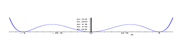
Figure 1: The potential (21) as function of the Higgs field.

In this case, the use of eq. (18) (with $c=1$) provides the result

$$A=1-h^{2},$$ (22)

which, substituting in (13), gives the solutions

$$h^{(+)}(x)=1/{\sqrt{1+e^{-2x}}}\,,\,A^{(-)}(x)=1/({1+e^{2x}}),$$ (23)

and

$$h^{(-)}(x)=1/{\sqrt{1+e^{2x}}}\,,\,A^{(+)}(x)=1/({1+e^{-2x}}),$$ (24)

which are displayed in fig. 2. We see that the scalar field, in both cases, interpolates between the symmetric and the asymmetric vacua.

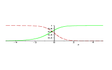
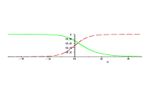
Figure 2: The Higgs field (solid line) and the gauge field (dashed line), $(h^{(+)}(x),A^{(-)}(x))$ from eq. (23) on the left, and $(h^{(-)}(x),A^{(+)}(x))$ from eq. (24) on the right.

fig. 3shows the energy and electric-charge densities for both wall solutions. We find that the spatial distribution of the electric charge is symmetric around the origin, while for the energy the axis of symmetry are displaced from the origin.

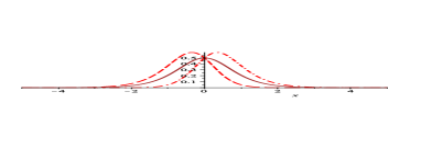
Figure 3: Energy density of the solutions $(h^{(+)}(x),A^{(-)}(x))$ (dashed line) and $(h^{(-)}(x),A^{(+)}(x))$ (dashed-dotted line), and module of electric-charge density for both solutions (solid line).

And, from eqs. (17), (19) and (20), for the solutions $(h^{(+)},A^{(-)})$ and $(h^{(-)},A^{(+)})$, we have the charges $Q=1$, $P=1/2$, and $Q=-1$, $P=-1/2$, respectively, and the same energy, $E=1$.

3 The deformation method

Let us now develop the deformation method for generalized Abelian HCS models following the spirit of the procedure introduced for scalar fields [15]. As we shall show, by deforming simultaneously the Higgs and the CS fields, we are able to construct many new generalized HCS models and their static domain-wall solutions. The original and the deformed models are mapped into each other through the deformation function.

Denote by $\tilde{\phi}(x)$ and $\widetilde{A}(x)$ new fields whose dynamics is governed by the (dimensionless) Lagrangian density

$$\widetilde{{\cal L}}=\widetilde{\omega}(|\tilde{\phi}|)|D_{\mu}\tilde{\phi}|^{2}-\widetilde{V}(|\tilde{\phi}|)+\frac{1}{4}\epsilon^{\alpha\beta\gamma}\widetilde{A}_{\alpha}\widetilde{F}_{\beta\gamma}\,,$$ (25)

where $\widetilde{V}(|\tilde{\phi}|)$ and $\widetilde{\omega}(|\tilde{\phi}|)$ are new functions specifying this model. As in sec. II, we assume that the self-dual BPS domain-wall solutions of this model take the form

$$\tilde{\phi}=\tilde{h}(x)\,,\,\,\,\,\,\,\widetilde{A}_{\mu}=\big{(}\widetilde{A}_{0}(x),\widetilde{A}_{1}=0,\widetilde{A}_{2}=\widetilde{A}(x)\big{)}\,,$$ (26)

and satisfy the first-order equations of motion

$$\tilde{h}^{\prime} = \pm\tilde{h}\widetilde{A}\,,$$ (27)

$$\widetilde{A}^{\prime} = -2\widetilde{\omega}\tilde{h}^{2}\widetilde{A}_{0}\,,$$ (28)

where $\tilde{h}^{\prime}\equiv{d\tilde{h}}/{dx}$ and $\widetilde{A}^{\prime}\equiv{d\widetilde{A}}/{dx}$, with the constraints $\widetilde{V}=h^{2}\widetilde{\omega}\widetilde{A}_{0}^{2}$ and $\widetilde{A}_{0}^{2}=\widetilde{A}^{2}$.

Now, introduce the deformation function $f$ such that the Higgs fields of the two models are mapped into each other, $h=f(\tilde{h})$, which is assumed to be invertible (in a prescribed domain of definition) and differentiable. Also, consider that the deformed CS-gauge field is obtained from $A$ by the prescription

$$\widetilde{A}(\tilde{h})=\frac{f(\tilde{h})\,A[h\rightarrow f(\tilde{h})]}{\tilde{h}f_{\widetilde{h}}}\,,$$ (29)

where $f_{\widetilde{h}}={df}/{d\widetilde{h}}$. Then, it follows from eqs. (27) and (28), using eq. (29), that the model defined by Lagrangian density (25), with the deformed function $\widetilde{\omega}$ and the deformed potential $\widetilde{V}$ given by

$$\widetilde{\omega}(\tilde{h})=\frac{1}{2}\frac{\widetilde{A}_{\tilde{h}}}{\tilde{h}}\,,\,\,\,\,\,\,\,\,\,\widetilde{V}(\tilde{h})=\tilde{h}^{2}\widetilde{A}^{2}\,\widetilde{\omega}(\tilde{h})\,,$$ (30)

where $\widetilde{A}_{\tilde{h}}=d\widetilde{A}/d\tilde{h}$, possesses static BPS solutions

$$\tilde{h}(x)=f^{-1}[h(x)]\,,\,\,\,\,\,\,\,\widetilde{A}(x)=\widetilde{A}\big{(}f^{-1}[h(x)]\big{)}\,,$$ (31)

where $h(x)$ is a static solution of the original model (1).

It should be noted that all the considerations and relations presented in sec. II, relative to energy and conserved charges, are held unchanged for the deformed system. In the following, taking as the starting point the JLW domain-wall solutions described in sec. II.A, we consider some illustrative examples of the method.

3.1 Example I

Firstly, we consider the couple of deformation function

$$f(\tilde{h})^{(\pm)}=(\pm)\frac{1-\tilde{h}^{2}}{1+\tilde{h}^{2}}\,,$$ (32)

which, using eqs. (22) and (29), gives $\widetilde{A}^{(\pm)}(\tilde{h})=f(\tilde{h})^{(\pm)}$; and, from eq. (30), it follows that

$$\tilde{\omega}=\frac{2}{(1+\tilde{h}^{2})^{2}}\,,\,\,\,\,\widetilde{V}=\frac{2\tilde{h}^{2}(1-\tilde{h}^{2})^{2}}{(1+\tilde{h}^{2})^{4}}\,.$$ (33)

These functions, which are plotted in fig. 4, define the generalized Abelian HCS model employed in Ref.[12]. Note that, the three vacua at $\tilde{h}=0,1,+\infty$ establish two walls, one between $\tilde{h}=0$ and $\tilde{h}=1$, and other between $\tilde{h}=1$ and $\tilde{h}=+\infty$.

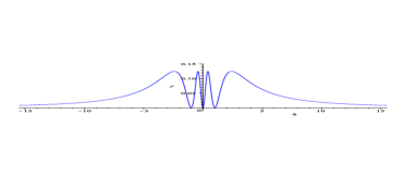
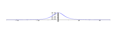
Figure 4: The potential (33) (top panel) and the corresponding function $w$ (bottom panel), as function of the Higgs field.

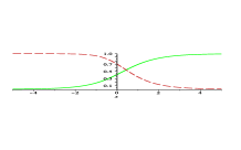
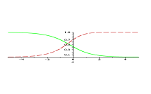
Figure 5: The Higgs field (solid line) and the gauge field (dashed line), $(\tilde{h}^{(+)}(x),\,\widetilde{A}^{(-)}(x))$ from eq. (LABEL:h1def1a) on the left, and $(\tilde{h}^{(-)}(x),\,\widetilde{A}^{(+)}(x))$ from eq. (35) on the right, for $0\leq\tilde{h}\leq 1$

From the inverse of the deformation function (32) and eqs. (23) and (24), for the range $0\leq\tilde{h}\leq 1$, we obtain the solutions

$$\tilde{h}^{(+)}(x) = \sqrt{1+e^{-2x}}-e^{-x}\,,\,\widetilde{A}^{(-)}(x)=1/{\sqrt{1+e^{2x}}}\,,$$

$$\tilde{h}^{(-)}(x) = 1/{\sqrt{1+2e^{2x}}}\,,\,\,\widetilde{A}^{(+)}(x)=1/{({1+e^{-2x}})},$$ (35)

while for $\tilde{h}\geq 1$ we have

$$\tilde{h}^{(+)}(x) = {\sqrt{1+2e^{2x}}}\,,\,\,\,\,\,\widetilde{A}^{(+)}(x)=1/({{1+e^{-2x}}})\,,$$ (36)

$$\tilde{h}^{(-)}(x) = \sqrt{1+e^{-2x}}+e^{-x}\,,\,\,\widetilde{A}^{(-)}(x)=1/({\sqrt{1+e^{2x}}}).$$

In figs. 5 and 6, we display these domain wall solutions. The walls for $0\leq\tilde{h}\leq 1$ and $\tilde{h}\geq 1$ have the same gauge fields, but with the asymptotic value for $x=\pm\infty$ changed. Then, for both ranges the walls have the same energy, $E=1$, and charges $Q=1$ and $P=1/2$, for $\widetilde{A}^{(-)}$, and $Q=-1$ and $P=-1/2$, for $\widetilde{A}^{(+)}$. This makes possible to have attractive or repulsive force between the two walls.

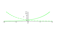
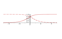
Figure 6: The fields $(\tilde{h}^{(+)}(x),\,\widetilde{A}^{(+)}(x))$, eq. (36) (solid line), and $(\tilde{h}^{(-)}(x),\,\widetilde{A}^{(-)}(x))$, eq. (LABEL:h2def1b) (dashed line), for $\tilde{h}\geq 1$.

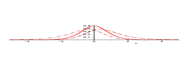
Figure 7: Module of electric charge for solutions $A^{(-)}(x)$ (dashed line) and $A^{(+)}(x)$ (dashed-dotted line), and energy density (solid line) for both walls.

In fig. 7, we display the energy and charge densities for the two walls. The comparison with the walls of the JLW model shows that, notwithstanding the walls have the same charges and energy, the JLW walls have symmetric spatial distributions of energy and charge, while here only the distribution of energy is symmetric and all the corresponding distributions are more spread out. The model defined by eqs. (33), which was obtained by deforming the JLW model, was studied in Ref. [12] but only the solution satisfying $0\leq\tilde{h}\leq 1$ was considered.

The deformation function (32) is a particular case of the deformation function $f(\tilde{h})=\cos[\alpha\arctan(\tilde{h})]$, corresponding to $\alpha=2$; from that new family of models can be generated for $\alpha$ integer.

3.2 Example II

As a second example, consider the set of deformation functions [16]

$$f_{\alpha}(\tilde{h})]=\cos[\alpha\,\arccos(\tilde{h})]=T_{\alpha}(\tilde{h})\,,$$ (38)

where the integer $\alpha>2$ and $T_{\alpha}$ is the Chebyshew polynomials of first kind. Using this deformation in eq. (29), with eq. (22), we have the gauge field

$$\widetilde{A}_{\alpha}(\tilde{h}) = ({1-\tilde{h}^{2}})^{1/2}\,\sin[2\alpha\,{\rm arccos}(\tilde{h})]\,/{2\alpha\tilde{h}}\,,$$ (39)

$$= {{(1-\tilde{h}^{2}})}\,U_{2\alpha-1}(\tilde{h})\,/{2\alpha\tilde{h}}\,,$$

where $U$ is the Chebyshew polynomials of second kind; which explicit results, for $\alpha=2,3$, are

$$\widetilde{A}_{2}(\tilde{h}) = (1-\tilde{h}^{2})(2\tilde{h}^{2}-1)\,,$$ (40)

$$\widetilde{A}_{3}(\tilde{h}) = \frac{1}{3}(1-\tilde{h}^{2})(1-2\tilde{h}^{2})(3-4\tilde{h}^{2})\,.$$ (41)

In this case, from eqs. (30) and (38), we have a family of models defined by the function $\widetilde{\omega}_{\alpha}(\tilde{h})$ and the potential $\widetilde{V}_{\alpha}(\tilde{h})$ written in polynomial form as

$$\widetilde{\omega}_{\alpha}(\tilde{h}) = |\,[2\alpha\tilde{h}\,T_{2\alpha}(\tilde{h})+U_{2\alpha-1}(\tilde{h})]/{4\alpha\tilde{h}^{3}}\,|\,,$$ (42)

$$\widetilde{V}_{\alpha}(\tilde{h}) = {(1-\tilde{h}^{2})^{2}}\,U^{2}_{2\alpha-1}(\tilde{h})\,\widetilde{\omega}_{\alpha}(\tilde{h})/{4\alpha^{2}}\,.$$ (43)

Then, each value of the parameter $\alpha$ specifies a model of this family. The explicit results for $\alpha=2,3$ are

$$\widetilde{\omega}_{2}(\tilde{h}) = 3-4\tilde{h}^{2}\,,$$ (44)

$$\widetilde{V}_{2}(\tilde{h}) = \tilde{h}^{2}(1-\tilde{h}^{2})^{2}(1-2\tilde{h}^{2})^{2}\,\widetilde{\omega}_{2}(\tilde{h})\,,$$ (45)

$$\widetilde{\omega}_{3}(\tilde{h}) = \frac{1}{3}(19-64\tilde{h}^{2}+48\tilde{h}^{4})\,,$$ (46)

$$\widetilde{V}_{3}(\tilde{h}) = \frac{1}{9}\tilde{h}^{2}(1-\tilde{h}^{2})^{2}(1-2\tilde{h}^{2})^{2}(3-4\tilde{h}^{2})^{2}\,\widetilde{\omega}_{3}(\tilde{h})\,.$$

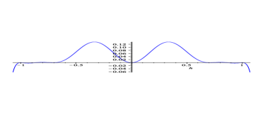
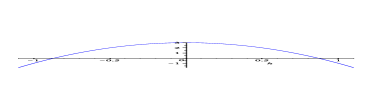
Figure 8: The potential (45) (top panel) and the function $w$ (44) (bottom panel), as function of $\tilde{h}$.

For these models, from the inverse of deformation function (38), we obtain the static Higgs field solutions in the form

$$\tilde{h}^{(\pm)}(x)=\cos\left[({\arccos(h^{(\pm)}(x))+(m-1)\pi})/{\alpha}\right]\,,$$ (48)

where $h^{(\pm)}(x)$ is given by eqs. (23) and (24), and $m$ is an integer, which generates distinct solutions only for $m=0,...,\alpha-1$ .

Firstly, we examine the model for $\alpha=2$, defined by eqs. (44) and (45) displayed in fig. 8. We see that, the potential is positive only for $\tilde{h}\leq\sqrt{3/2}$. Then, there are two kind of static solutions for the Higgs field, one pair kink/anti-kink like solution between $0\leq\tilde{h}\leq 1/\sqrt{2}$, and a lump-like solution between $1/\sqrt{2}\leq\tilde{h}\leq\sqrt{3/2}$. In Ref. [21] is considered a model that presents a charged lump-like solution. Here, the lump-like solution presents vanishing charges and energy, hence we examine only the wall for $0\leq\tilde{h}\leq 1/\sqrt{2}$. In fig. 9, we display the Higgs field (48) and the gauge field (39) solutions. These walls have the same total energy and charges of the walls of the standard JLW model, but with different spacial distribution of the energy and charge densities, as shown in fig. 10.

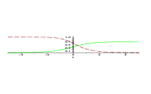
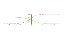
Figure 9: The Higgs field (48) for $m=0$ (solid line) and the matching gauge field (40) (dashed line), for $\tilde{h}^{(+)}(x)$ and $\widetilde{A}^{(-)}(x)$, on the left, and for $\tilde{h}^{(-)}(x)$ and $\widetilde{A}^{(+)}(x)$, on the right.

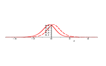
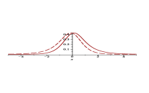
Figure 10: The energy density (on the left) and the module of charge density (on the right), for solution $A^{(-)}(x)$ (solid line), and for $A^{(+)}(x)$ (dashed-line).

4 Ending Comments

The examples presented above illustrate how the deformation method may be used to generate many new generalized Abelian HCS models and their defect solutions. This is achieved without requiring to directly solve the nonlinear equations of motion of the new models. The method also allows the construction of new defect solutions controlling important features such as their height, width or the topological character. Such results are of direct interest to applications of domain walls in several contexts, such as high-energy or condensed-matter physics.

- [1] \NameRajaraman R. \BookSolitons and Instantons \PublNorth Holland, Amsterdam \Year1982; \NameRebbi C. Soliani G. \BookSolitons and Particles \PublWorld Scientific, Singapore \Year1984.
- [2] \NameVilenkin A. Shellard E. P. S. \BookCosmic Strings, and Other Topological Defects \PublCambridge UP, Cambridge/UK \Year1994.
- [3] \NameEschenfelder A. H. \BookMagnetic Bubble Technology \PublSpringer, New York \Year1997.
- [4] \NameLerda A. \BookAnyons: Quantum Mechanics of Particles with Fractional Statistics \PublSpringer-Verlag, Berlin \Year1992.
- [5] \NameHagen C. R. \REVIEWPhys. Rev. D311985848.
- [6] \NameJackiw R. Pi S.-Y. \REVIEWPhys. Rev. D4219903500.
- [7] \NameBergman O. Lozano G. \REVIEWAnn. Phys. (NY)2291994416.
- [8] \NameGomes M., Malbouisson J. M. C. da Silva A. J. \REVIEWPhys. Lett. A2361997373; \NameGomes M., Malbouisson J. M. C., Rodrigues A. G. da Silva A. J. \REVIEWJ. Phys. A: Math. Gen.3320005521.
- [9] \NameHong J., Kim Y. Pac P. Y. \REVIEWPhys. Rev. Lett.6419902230; \NameJackiw R. Weinberg E. J. \REVIEWPhys. Rev. Lett.6419902234.
- [10] \NameJackiw R., Lee K. Weinberg E. J. \REVIEWPhys. Rev. D4219903488.
- [11] \NameBazeia D., da Hora E., dos Santos C. Menezes R. \REVIEWPhys. Rev. D812010125014.
- [12] \Namedos Santos C. da Hora E. \REVIEWEur. Phys. J. C7020101145.
- [13] \NameSkyrme T. H. R. \REVIEWProc. R. Soc. London, Ser. A2601961127; \NameAratyn H., Ferreira L. A. Zimerman A. H. \REVIEWPhys. Rev. Lett.8319991723; \NameBabichev E. \REVIEWPhys. Rev. D742006085004; \NameAdam C., Klimas P., Sanchez-Guillen J. Wereszczynski A. \REVIEWJ. Phys. A422009135401.
- [14] \NameArmendariz-Picon C., Damour T. Mukhanov V. F. \REVIEWPhys. Lett. B4581999209; \NameGarriga J. Mukhanov V. F. \REVIEWPhys. Lett. B4581999219; \NameChiba T., Okabe T. Yamaguchi M. \REVIEWPhys.Rev. D622000023511; \NameVerbin Y., Madsen S. Larsen A. L. \REVIEWPhys. Rev. D672003085019; \NameArmendariz-Picon C. Lim E. A. \REVIEWJCAP05082005007; \NameRendall A. D. \REVIEWClass. Quant. Grav.2320061557.
- [15] \NameBazeia D., Losano L. Malbouisson J. M. C. \REVIEWPhys.Rev. D662002101701(R); \NameAlmeida C. A., Bazeia D., Losano L. Malbouisson J. M. C. \REVIEWPhys. Rev. D692004067702; \NameBazeia D. Losano L. \REVIEWPhys. Rev. D732006025016.
- [16] \NameBazeia D., Gonzalez Leon M. A., Losano L. Mateos Guilarte J. \REVIEWPhys. Rev. D732006105008.
- [17] \NameBazeia D., Losano L., Malbouisson J. M. C. Menezes R. \REVIEWPhysica D2372008937; \NameBazeia D., Losano L., Menezes R. Souza M. A. M. \REVIEWEurophys. Lett.87200921001; \NameBazeia D., Losano L., Malbouisson J. M. C. Santos J. R. L. \REVIEWEur. Phys. J. C712011176.
- [18] \NameAfonso V. I., Bazeia D., Gonzalez Leon M. A., Losano L. Mateos Gilarte J. \REVIEWPhys. Rev. D762007025010.
- [19] \NameBogomol’nyi E. B. \REVIEWYad. Fiz.241976861 [\REVIEWSov. J. Nucl. Phys.241976449]; \NamePrasad M. Sommerfeld C. \REVIEWPhys. Rev. Lett.351975760.
- [20] \NameVega H. Schaposnik F. \REVIEWPhys. Rev. D1419761100.
- [21] \Namedos Santos C. da Hora E. \REVIEWEur. J. Phys. C7120111519.