Energy- and enstrophy-conserving schemes for the shallow-water equations, based on mimetic finite elements

Abstract

This paper presents a family of spatial discretisations of the nonlinear rotating shallow-water equations that conserve both energy and potential enstrophy. These are based on two-dimensional mixed finite element methods and hence, unlike some finite difference methods, do not require an orthogonal grid. Numerical verification of the aforementioned properties is also provided.

Keywords: mixed finite element; energy conservation; shallow-water equations

1 Introduction

The quest for scalable, massively parallel numerical weather prediction models has led to great interest in extensions of C-grid staggering to more general mesh structures, such as icosahedral and cubed meshes. There is also increasing interest in atmosphere and ocean models that allow arbitrary mesh refinement, in order to facilitate seamless regional modelling within a global model. C-grid staggering was proposed as a way of preventing spurious numerical wave propagation that appears on other grid staggerings (Sadourny, 1975; Arakawa and Lamb, 1977); these spurious waves interfere with geostrophic adjustment processes in the numerical solution and rapidly degrade predictive skill. It was known from the beginning that the C-grid staggering admits natural finite-difference differential operators (div, grad, curl) that satisfy discrete versions of vector calculus identities (div–curl = 0; curl–grad = 0). These identities allow a separation of the irrotational and solenoidal components of velocity, which play quite different roles in the low Rossby number regime.

It was also recognised, from experience with incompressible quasigeostrophic models (Arakawa, 1966), that conservation of energy and potential enstrophy are important for obtaining nonlinear stability of the model without excessive numerical diffusion. An energy-conserving formulation was provided in Sadourny (1975), and a formulation that conserves both energy and enstrophy was given in Arakawa and Lamb (1981). In the regime of quasigeostrophic turbulence, the shallow-water equations exhibit a cascade of energy to large scales. On the other hand, enstrophy cascades to small scales, and so it makes sense to attempt to dissipate enstrophy at small scales. The Anticipated Potential Vorticity Method (APVM) was introduced as a closure to represent the cascade to scales below the grid width (Sadourny and Basdevant, 1985); for an appropriate choice of parameters, the APVM is closely related to Lax–Wendroff advection schemes. The APVM was incorporated into an energy-conserving, enstrophy-dissipating shallow-water model in Arakawa and Hsu (1990); it remains useful to start with an enstrophy-conserving model and to then introduce an enstrophy-dissipating term, since one then has complete control over the enstrophy dynamics in the model. Arakawa and Hsu (1990) also demonstrated how to handle massless layers in this framework, which become the basis of many isopycnal ocean models (Hallberg and Rhines, 1996, for example).

On the sphere, the development of C-grid staggerings for grids other than the usual latitude-longitude grid was guided by the extension of the C-grid div, grad and curl operators to arbitrary grids by the mimetic finite difference community, and by the connection with finite volume methods (Hyman and Shashkov, 1997). One route towards energy- and enstrophy-conserving schemes was proposed using Nambu brackets (Salmon, 2005, 2007; Sommer and Névir, 2009; Gassmann and Herzog, 2008). In general, a key challenge was the design of reconstruction methods for the Coriolis term that allowed for steady linear geostrophic modes on the $f$-plane, without which nonlinear solutions near to geostrophic balance would spuriously couple with fast gravity waves. Such a reconstruction was apparent for triangular grids by making use of the Raviart-Thomas reconstruction (Bonaventura and Ringler, 2005), but unfortunately the triangular scheme suffers from spurious branches of inertia-gravity waves that render it problematic (Danilov, 2010; Gassmann, 2011).

A suitable reconstruction on hexagonal grids was then provided in Thuburn (2008) and extended to arbitrary orthogonal polygonal grids in Thuburn et al. (2009), and energy-conserving, enstrophy-dissipating schemes for the nonlinear shallow-water equations on arbitrary orthogonal grids were introduced in Ringler et al. (2010). As discussed in Staniforth and Thuburn (2012), the global degree-of-freedom ratio between velocity and pressure is altered by increasing or decreasing the number of cell edges. This may lead to spurious mode branches – spurious inertia-gravity wave branches are present for triangles and spurious Rossby mode branches, for hexagons – so quadrilaterals are preferred in order to minimise the possibility of spurious modes. This suggests the cube mesh for modelling on the sphere. Unfortunately, the orthogonality requirement in the construction of Thuburn et al. (2009) leads to meshes that cluster resolution around the cube vertices, which leads to non-uniform parallel communication requirements. This led Thuburn and Cotter (2012) to extend the framework of Thuburn et al. (2009) to non-orthogonal grids. It has since been discovered that the scheme of Thuburn et al. (2009) on the dual icosahedral grid and the scheme of Thuburn and Cotter (2012) on the cube grid both have inconsistent discretisations of the Coriolis term (Thuburn, personal communication), meaning that grid refinement does not improve the accuracy of this term. This, together with the additional flexibility to alter degree-of-freedom ratios and to increase the order of accuracy, has motivated the investigation of mixed finite element methods.

Mixed finite element methods are the analogue of staggered grids since they use different finite element spaces for velocity and pressure. Many different combinations of finite element spaces have been examined in the ocean modelling literature (Le Roux, 2005; Le Roux et al., 2007; Rostand and Le Roux, 2008; Le Roux and Pouliot, 2008; Le Roux et al., 2009; Danilov et al., 2008; Comblen et al., 2010; Cotter and Ham, 2011; Le Roux, 2012). Cotter and Shipton (2012) concentrated on combinations of spaces that have discrete versions of the div–curl and curl–grad identities, just like the C-grid. In the numerical analysis literature, this is referred to as “finite element exterior calculus” (Arnold et al., 2006). These combinations were shown to provide all the properties of the C-grid staggering, including steady linear geostrophic modes on the $f$-plane, and hence merited further investigation (Cotter and Shipton, 2012). Staniforth et al. (2012) examined wave propagation for one particular combination, namely the 2nd order Raviart–Thomas ($\mathrm{RT}_{1}$) space for velocity and the bilinear discontinuous ($\mathrm{Q}_{1}^{\mathrm{DG}}$) space for pressure, and observed a $2\Delta x$ mode with zero group velocity; this mode can be corrected by partially lumping the velocity mass matrix.

In this paper we provide a formulation that uses mixed finite elements of the type proposed in Cotter and Shipton (2012). The formulation closely follows the steps of Ringler et al. (2010): the prognostic variables are velocity and layer depth, but there is a diagnostic potential vorticity that satisfies a discrete conservation law. Using this potential vorticity in the vector-invariant form of the equations (as used in the classical C-grid development) naturally leads to an energy- and enstrophy-conserving form of the equations without further modification. The conservation properties arise from the mimetic properties combined with the integral formulation. We introduce a finite element version of the APVM that dissipates enstrophy at the gridscale. This formulation is illustrated through numerical experiments that demonstrate the energy and enstrophy properties, and demonstrate that the numerical scheme is convergent and stable. The analytic shallow-water equations and a selection of derived results are given in section 2. We give our proposed spatial discretisation in section 3. Numerical validation is presented in section 4, and further areas of research are discussed in the conclusion. We close by demonstrating that the conservation properties arise from an almost-Poisson structure of the spatially discretised equations; this is in Appendix A.

2 Analytic Formulation

In this section, we review conservation properties of the rotating shallow-water equations, since their proofs will be extended to the finite element discretisations in section 3.

The nonlinear shallow-water equations in a rotating frame of reference are commonly written as

$$\frac{\partial\mathbf{u}}{\partial t}+(\mathbf{u}\cdot\nabla)\mathbf{u}+f\mathbf{u}^{\perp} =-g\nabla h\ ,$$ (2.1)

$$\frac{\partial h}{\partial t}+\nabla\cdot(h\mathbf{u}) =0\ ,$$ (2.2)

where ${\mathbf{u}(x,y,t)}$ is the velocity, ${h(x,y,t)}$ is the layer depth, ${f(x,y)}$ is the Coriolis parameter, and $g$ is the gravitational acceleration. We introduce the ^⟂ notation for brevity: for a two-dimensional vector $\mathbf{w}$ in the ${x\text{-}y}$ plane, ${\mathbf{w}^{\perp}=\hat{\mathbf{z}}\times\mathbf{w}}$, a 90^∘ counterclockwise rotation. If $\mathbf{w}$ is a vector field, this is done pointwise. We will also use the notation ${\nabla^{\perp}}$ and ${\nabla^{\perp}\cdot}$: writing $\nabla$ in components as ${(\partial_{x},\partial_{y})}$, we have ${\nabla^{\perp}=(-\partial_{y},\partial_{x})}$. If $\gamma$ is a scalar field,

$$\nabla^{\perp}\gamma=\left(-\frac{\partial\gamma}{\partial y},\frac{\partial\gamma}{\partial x}\right)\ .$$ (2.3)

For a vector field $\mathbf{w}$, with ${\mathbf{w}\equiv(u,v)}$ in components,

$$\nabla^{\perp}\!\cdot\mathbf{w}=\frac{\partial v}{\partial x}-\frac{\partial u}{\partial y}\ ,$$ (2.4)

a two-dimensional form of $\nabla\times$.

When rewritten in terms of the relative vorticity ${\zeta=\nabla^{\perp}\!\cdot\mathbf{u}\equiv\hat{\mathbf{z}}\cdot\nabla\times\mathbf{u}}$, (2.1) and (2.2) become

$$\frac{\partial\mathbf{u}}{\partial t}+(\zeta+f)\mathbf{u}^{\perp}+\nabla\left(gh+\frac{1}{2}|\mathbf{u}|^{2}\right) =0\ ,$$ (2.5)

$$\frac{\partial h}{\partial t}+\nabla\cdot(h\mathbf{u}) =0\ .$$ (2.6)

This is the so-called ‘vector-invariant’ form of the equations, which is the starting point for energy- or enstrophy-conserving formulations using the C-grid staggering; we shall also use this form here.

We can derive a continuity equation for the absolute vorticity ${\zeta+f}$. Defining a potential vorticity ${q=\frac{\zeta+f}{h}}$, we rewrite (2.5):

$$\frac{\partial\mathbf{u}}{\partial t}+qh\mathbf{u}^{\perp}+\nabla\left(gh+\frac{1}{2}|\mathbf{u}|^{2}\right) =0\ .$$ (2.7)

We now apply the $${\nabla^{\perp}\cdot}$$ operator to (2.7), giving

$$\frac{\partial}{\partial t}(\nabla^{\perp}\!\cdot\mathbf{u})+\nabla^{\perp}\!\cdot(qh\mathbf{u}^{\perp}) =0\ ,$$ (2.8)

$$\implies\frac{\partial\zeta}{\partial t}+\nabla\cdot(qh\mathbf{u}) =0\ .$$ (2.9)

Assuming ${\frac{\partial f}{\partial t}=0}$, we then have

$$\frac{\partial}{\partial t}(qh)+\nabla\cdot(qh\mathbf{u})=0\ ,$$ (2.10)

which is the equation for $q$ written in local conservation form. From this, we can derive an advection equation for the potential vorticity $q$. Recall the continuity equation (2.6). Multiplying this by $q$, and comparing with (2.10), we obtain

$$h\left[\frac{\partial q}{\partial t}+(\mathbf{u}\cdot\nabla)q\right]=0\ ,$$ (2.11)

implying that $q$ remains constant in a Lagrangian frame moving with fluid particles. In particular, if $q$ is initially uniform, $q$ will remain uniform (and constant) for all time.

In a boundary-free domain, several quantities are conserved. Integrating (2.10) over the whole domain gives conservation of the total absolute vorticity ${\int_{A}\!qh\,\mathrm{d}A}$. Less trivially, the total enstrophy ${\int_{A}\!q^{2}h\,\mathrm{d}A}$ and the total energy ${\int_{A}\!\left[\frac{1}{2}h|\mathbf{u}|^{2}+\frac{1}{2}gh^{2}\right]\,\mathrm{d}A}$ are also constant.

The conservation of enstrophy follows from direct manipulation:

$$\frac{\mathrm{d}}{\mathrm{d}t}\int_{A}\!q^{2}h\,\mathrm{d}A =\int_{A}\!\left[2q\frac{\partial}{\partial t}(qh)-q^{2}\frac{\partial h}{\partial t}\right]\,\mathrm{d}A$$ (2.12)

$$=\int_{A}\!\left[2q\nabla\cdot(-qh\mathbf{u})-q^{2}\nabla\cdot(-h\mathbf{u})\right]\,\mathrm{d}A$$ (2.13)

$$=-\int_{A}\!\nabla\cdot(q^{2}h\mathbf{u})\,\mathrm{d}A$$ (2.14)

$$=0\ ,$$

where we have used (2.10) and (2.6) between the first and second line. A similar result for higher order moments of potential vorticity can be obtained by replacing $q^{2}$ with $q^{m}$.

Similarly, conservation of energy follows from

$$\frac{\mathrm{d}}{\mathrm{d}t}\int_{A}\!\left[\frac{1}{2}h|\mathbf{u}|^{2}+\frac{1}{2}gh^{2}\right]\,\mathrm{d}A$$

$$\qquad\qquad=\int_{A}\!\left[h\frac{\partial}{\partial t}\left(\frac{1}{2}|\mathbf{u}|^{2}\right)+\frac{1}{2}|\mathbf{u}|^{2}\frac{\partial h}{\partial t}+gh\frac{\partial h}{\partial t}\right]\,\mathrm{d}A$$ (2.15)

$$\qquad\qquad=\int_{A}\!\left[h\frac{\partial}{\partial t}\left(\frac{1}{2}|\mathbf{u}|^{2}\right)+\left(\frac{1}{2}|\mathbf{u}|^{2}+gh\right)\frac{\partial h}{\partial t}\right]\,\mathrm{d}A$$ (2.16)

$$\qquad\qquad=\int_{A}\!\left[-h\mathbf{u}\cdot\nabla\left(\frac{1}{2}|\mathbf{u}|^{2}+gh\right)-\left(\frac{1}{2}|\mathbf{u}|^{2}+gh\right)\nabla\cdot(h\mathbf{u})\right]\,\mathrm{d}A$$ (2.17)

$$\qquad\qquad=-\int_{A}\!\nabla\cdot\left[h\mathbf{u}\left(\frac{1}{2}|\mathbf{u}|^{2}+gh\right)\right]\,\mathrm{d}A$$ (2.18)

$$\qquad\qquad=0\ ,$$

where we have used $\mathbf{u}\cdot$(2.5) and (2.6) between the third and fourth line.

3 Finite Element Discretisation

In this section, we present a family of spatial discretisations, based on the Finite Element Method, for the nonlinear rotating shallow-water equations. These discretisations will mimic many properties of the continuous equations, including the conservation of enstrophy and energy. The prognostic variables will be the velocity field $\mathbf{u}$ and the layer depth $h$. Our method explicitly defines a potential vorticity field $q$ and a volume flux $\mathbf{F}$. However, these should be interpreted as diagnostic functions of $\mathbf{u}$ and $h$, rather than independent variables in their own right.

The critical step is the choice of function spaces in which our fields will reside. In the Finite Element Method, the domain is partitioned into a large number of non-overlapping subdomains (elements). The function space specification can be divided into two parts: the behaviour of a function within each element, and the continuity of a function at the element boundaries. Almost all function spaces are piecewise-polynomial (that is, a polynomial when restricted to a single element). For a scalar function space, the most common continuity constraints are:

• $C^{0}$ continuous - giving the Continuous Galerkin family ${\mathrm{P}}_{n}$, where $n$ is the polynomial degree, and

• discontinuous - giving the Discontinuous Galerkin family ${\mathrm{P}}_{n}^{\mathrm{DG}}$, where $n$ is the polynomial degree.

Other, less common, conditions include $C^{1}$ continuity between elements, and nonconforming ($C^{0}$ continuity at only the midpoint of edges). The Continuous and Discontinuous Galerkin families are somewhat natural function spaces for scalar fields; this can be stated more precisely in the context of finite element exterior calculus (Arnold et al., 2006). Commonly-used vector function spaces are often merely tensor products of these two types of scalar function spaces. However, a careless choice of function space can lead to genuinely incorrect results, such as spurious solutions arising in eigenvalue problems (Arnold et al., 2010).

We now introduce the function spaces that we will use, and the relations between them; further details can be found in Cotter and Shipton (2012). We make use of a family of partially discontinuous vector spaces which are contained in H(div), in other words they are ‘div-conforming’:

$$\int_{A}\!\mathbf{u}\cdot\mathbf{u}+(\nabla\cdot\mathbf{u})(\nabla\cdot\mathbf{u})\,\mathrm{d}A<\infty\ .$$ (3.1)

Since the functions will be piecewise-polynomial, this condition can only be violated due to behaviour at element boundaries. The normal component of the vector field must therefore be continuous across element boundaries, although the tangential component may be discontinuous (there is a related space H(curl) in which the opposite is true). Our velocity field $\mathbf{u}$ and volume flux $\mathbf{F}$ will live in this space, which we will denote $\mathrm{S}$. Examples include the Raviart–Thomas family $\mathrm{RT}_{n}$ (Raviart and Thomas, 1977), the Brezzi–Douglas–Marini family $\mathrm{BDM}_{n}$ (Brezzi et al., 1985), and the Brezzi–Douglas–Fortin–Marini family $\mathrm{BDFM}_{n}$ (Brezzi and Fortin, 1991).

For each choice of $\mathrm{S}$, we can define a scalar function space

$$\mathrm{V}=\left\{\nabla\cdot\mathbf{w}:\mathbf{w}\in\mathrm{S}\right\}\ .$$ (3.2)

This space is totally discontinuous at element boundaries. The layer depth $h$ will be in $\mathrm{V}$. Finally, following principles of Finite Element Exterior Calculus, we define a function space $\mathrm{E}$ such that

$$\nabla^{\perp}\mathrm{E}\equiv\{\nabla^{\perp}\gamma\colon\gamma\in\mathrm{E}\}\subset\mathrm{S}\ ,$$ (3.3)

and

$$\nabla^{\perp}\mathrm{E}=\left\{\ker(\nabla\cdot\colon\mathrm{S}\to\mathrm{V})\right\}\ ;$$ (3.4)

$\nabla^{\perp}$ maps bijectively from $\mathrm{E}$ to ${\{\ker(\nabla\cdot)\}\subset\mathrm{S}}$, modulo constant functions. This ensures that, for any ${\gamma\in\mathrm{E}}$, ${\nabla\cdot\nabla^{\perp}\gamma\equiv 0}$, the zero-function in $\mathrm{V}$, and is the analogue of the continuous identity ${\nabla\cdot\nabla\times\equiv 0}$. $\mathrm{E}$ is continuous at element boundaries, and will contain the potential vorticity field $q$.

We refer to the ${\nabla^{\perp}\colon\mathrm{E}\to\mathrm{S}}$ and ${\nabla\cdot\colon\mathrm{S}\to\mathrm{V}}$ operators as ‘strong’ derivatives, since they act in a pointwise sense and are identical to the ‘continuous’ $\nabla^{\perp}$ and $\nabla\cdot$ operators. There are corresponding ‘weak’ operators ${\widetilde{\nabla}^{\perp}\cdot\colon\mathrm{S}\to\mathrm{E}}$ and ${\widetilde{\nabla}\colon\mathrm{V}\to\mathrm{S}}$ which do not act pointwise, but are instead defined via integration by parts. Before we elaborate, we take the opportunity to introduce some notation. We will use angle brackets to denote the standard $L^{2}$ inner product:

$$\left\langle f,g\right\rangle=\int_{A}\!f(x^{\prime})g(x^{\prime})\,\mathrm{d}A\ ,\qquad\left\langle\mathbf{u},\mathbf{v}\right\rangle=\int_{A}\!\mathbf{u}(x^{\prime})\cdot\mathbf{v}(x^{\prime})\,\mathrm{d}A\ .$$ (3.5)

Then, in a domain without boundaries, we define $\widetilde{\nabla}^{\perp}\cdot$ and $\widetilde{\nabla}$ by

$$\left\langle\gamma,\widetilde{\nabla}^{\perp}\!\cdot\mathbf{u}\right\rangle=-\left\langle\nabla^{\perp}\gamma,\mathbf{u}\right\rangle\ ,\quad\forall\gamma\in\mathrm{E}\ ,$$ (3.6)

$$\left\langle\mathbf{w},\widetilde{\nabla}h\right\rangle=-\left\langle\nabla\cdot\mathbf{w},h\right\rangle\ ,\quad\forall\mathbf{w}\in\mathrm{S}\ .$$ (3.7)

This is a surprisingly natural definition: let $\Pi_{\mathrm{E}},\Pi_{\mathrm{S}},\Pi_{\mathrm{V}}$ be operators that $L^{2}$-project arbitrary functions into $\mathrm{E}$, $\mathrm{S}$ and $\mathrm{V}$ respectively, i.e.

$$\left\langle\gamma,\Pi_{\mathrm{E}}(f)\right\rangle=\left\langle\gamma,f\right\rangle\ ,\quad\forall\gamma\in\mathrm{E}\ ,$$ (3.8)

with $\Pi_{\mathrm{S}}$ and $\Pi_{\mathrm{V}}$ defined analogously. Then the following identities hold:

$$\widetilde{\nabla}^{\perp}\!\cdot(\Pi_{\mathrm{S}}(\mathbf{v}))\equiv\Pi_{\mathrm{E}}(\nabla^{\perp}\!\cdot\mathbf{v})\ ,$$ (3.9)

$$\widetilde{\nabla}(\Pi_{\mathrm{V}}(f))\equiv\Pi_{\mathrm{S}}(\nabla f)\ ,$$ (3.10)

where $\mathbf{v}$ and $f$ are arbitrary functions; the weak differential operators commute with $L^{2}$ projection into the function spaces. These identities underlie the proof of steady linear geostrophic modes in the $f$-plane outlined in Cotter and Shipton (2012).

We are now ready to present the discretisation. Recall that $\mathbf{u}$ is in $\mathrm{S}$ and $h$ is in $\mathrm{V}$. The continuous potential vorticity $q$ satisfied ${qh=\zeta+f}$, where ${\zeta=\nabla^{\perp}\!\cdot\mathbf{u}}$. However, this is invalid in our discrete framework: for ${\mathbf{u}\in\mathrm{S}}$, ${\nabla^{\perp}\!\cdot\mathbf{u}}$ is not generally defined, since the tangential component of $\mathbf{u}$ is not continuous across element boundaries. Instead, we must use the weak operator $\widetilde{\nabla}^{\perp}\cdot$ discussed previously. Our discrete potential vorticity ${q\in\mathrm{E}}$ is therefore defined to satisfy, in a boundary-free domain,

$$\left\langle\gamma,qh\right\rangle=\left\langle-\nabla^{\perp}\gamma,\mathbf{u}\right\rangle+\left\langle\gamma,f\right\rangle,\quad\forall\gamma\in\mathrm{E}\ .$$ (3.11)

In a domain with boundaries, we would pick up a non-vanishing surface integral when integrating by parts.

In the continuity equation (2.6), there was a term ${\nabla\cdot(h\mathbf{u})}$. Since ${h\in\mathrm{V}}$ is discontinuous, this expression is problematic. In order to write a discrete continuity equation, we define a discrete volume flux $\mathbf{F}$ to be the $L^{2}$ projection of $h\mathbf{u}$ into $\mathrm{S}$, i.e.

$$\left\langle\mathbf{w},\mathbf{F}\right\rangle=\left\langle\mathbf{w},h\mathbf{u}\right\rangle\ ,\quad\forall\mathbf{w}\in\mathrm{S}\ .$$ (3.12)

We can then replace ${\nabla\cdot(h\mathbf{u})}$ by ${\nabla\cdot\mathbf{F}}$.

Similarly, in the momentum equation (2.7), there was a term ${\nabla\left(gh+\frac{1}{2}|\mathbf{u}|^{2}\right)}$, which is again incompatible with our discrete framework. We replace $\nabla$ by the weak gradient $\widetilde{\nabla}$ discussed previously. The discrete forms of our evolution equations (2.5) and (2.6) are then

$$\left\langle\mathbf{w},\frac{\partial\mathbf{u}}{\partial t}\right\rangle+\left\langle\mathbf{w},q\mathbf{F}^{\perp}\right\rangle-\left\langle\nabla\cdot\mathbf{w},gh+\frac{1}{2}|\mathbf{u}|^{2}\right\rangle =0\ ,\quad\forall\mathbf{w}\in\mathrm{S}\ ,$$ (3.13)

$$\left\langle\phi,\frac{\partial h}{\partial t}\right\rangle+\left\langle\phi,\nabla\cdot\mathbf{F}\right\rangle =0\ ,\quad\forall\phi\in\mathrm{V}\ .$$ (3.14)

The equations (3.11) through (3.14) form our scheme. Note that (3.13) holds even in a domain with boundaries, as long as ${\mathbf{u}\cdot\mathbf{n}=0}$. More importantly, (3.14) implies that the equation

$$\frac{\partial h}{\partial t}+\nabla\cdot\mathbf{F}=0$$ (3.15)

is satisfied pointwise, as both $\frac{\partial h}{\partial t}$ and $\nabla\cdot\mathbf{F}$ are in $\mathrm{V}$.

In a boundary-free domain, these discrete equations reproduce the results given in the previous section for the continuous governing equations. Recalling that ${\nabla\cdot\nabla^{\perp}\gamma\equiv 0}$, we begin by inserting ${\mathbf{w}=-\nabla^{\perp}\gamma}$ into (3.13), for any ${\gamma\in\mathrm{E}}$:

$$\left\langle-\nabla^{\perp}\gamma,\frac{\partial\mathbf{u}}{\partial t}\right\rangle+\left\langle-\nabla^{\perp}\gamma,q\mathbf{F}^{\perp}\right\rangle=0\ ,\quad\forall\gamma\in\mathrm{E}\ .$$ (3.16)

Assuming that ${\frac{\partial f}{\partial t}=0}$, we can rewrite the first term using $\frac{\partial}{\partial t}$(3.11):

$$\left\langle\gamma,\frac{\partial}{\partial t}(qh)\right\rangle+\left\langle-\nabla^{\perp}\gamma,q\mathbf{F}^{\perp}\right\rangle =0\ ,\quad\forall\gamma\in\mathrm{E}$$ (3.17)

$$\implies\left\langle\gamma,\frac{\partial}{\partial t}(qh)\right\rangle+\left\langle-\nabla\gamma,q\mathbf{F}\right\rangle =0\ ,\quad\forall\gamma\in\mathrm{E}$$ (3.18)

$$\implies\left\langle\gamma,\frac{\partial}{\partial t}(qh)\right\rangle+\left\langle\gamma,\nabla\cdot(q\mathbf{F})\right\rangle =0\ ,\quad\forall\gamma\in\mathrm{E}\ ,$$ (3.19)

where the integration by parts in the final line is permitted, i.e. it is an exact identity, since $\gamma$ is continuous and $\mathbf{F}$ is div-conforming. (3.19) is a discrete approximation to the local conservation law for $q$ (2.10), which was previously combined with the continuity equation to form an advection equation or $q$ (2.11). A similar procedure can be carried out in the discrete case by expanding out the derivatives:

$$\left\langle\gamma,h\frac{\partial q}{\partial t}+q\frac{\partial h}{\partial t}\right\rangle+\left\langle\gamma,q\nabla\cdot\mathbf{F}+(\mathbf{F}\cdot\nabla)q\right\rangle=0,\quad\forall\gamma\in\mathrm{E}\ .$$ (3.20)

We now use our observation (3.15), which stated that the continuity equation holds pointwise, implying

$$\left\langle\gamma,h\frac{\partial q}{\partial t}\right\rangle+\left\langle\gamma,(\mathbf{F}\cdot\nabla)q\right\rangle=0,\quad\forall\gamma\in\mathrm{E}\ .$$ (3.21)

This is a discrete analogue of (2.11), and is enough to reproduce the result that if $q$ is initially constant, $q$ remains constant for all time.

To reproduce conservation laws, we will typically make a specific choice of the ‘test-function’ $\gamma$ (or $\mathbf{w}$, or $\phi$). For example, taking ${\gamma\equiv 1}$ in (3.17) or (3.18) gives conservation of absolute vorticity in a boundary-free domain.

Conservation of enstrophy follows from choosing ${\gamma=q}$ (which is permitted since ${q\in E}$):

$$\frac{\mathrm{d}}{\mathrm{d}t}\int_{A}\!q^{2}h\,\mathrm{d}A \equiv\frac{\mathrm{d}}{\mathrm{d}t}\left\langle q,qh\right\rangle$$ (3.22)

$$=2\left\langle q,\frac{\partial}{\partial t}(qh)\right\rangle-\left\langle q^{2},\frac{\partial h}{\partial t}\right\rangle\ .$$ (3.23)

Using our result from (3.15), that $${\frac{\partial h}{\partial t}+\nabla\cdot\mathbf{F}=0} {\gamma=q}$$ is satisfied pointwise, and taking in (3.18):

$$=2\left\langle\nabla q,q\mathbf{F}\right\rangle+\left\langle q^{2},\nabla\cdot\mathbf{F}\right\rangle$$ (3.24)

$$=\int_{A}\!\nabla\cdot(q^{2}\mathbf{F})\,\mathrm{d}A$$ (3.25)

$$=0\ .$$

Conservation of energy is again obtained by direct computation:

$$\frac{\mathrm{d}}{\mathrm{d}t}\int_{A}\!\left[\frac{1}{2}h|\mathbf{u}|^{2}+\frac{1}{2}gh^{2}\right]\,\mathrm{d}A\equiv\frac{\mathrm{d}}{\mathrm{d}t}\left(\frac{1}{2}\left\langle h\mathbf{u},\mathbf{u}\right\rangle+\frac{1}{2}\left\langle gh,h\right\rangle\right)$$ (3.26)

$$\qquad\qquad=\left\langle h\mathbf{u},\frac{\partial\mathbf{u}}{\partial t}\right\rangle+\left\langle\frac{\partial h}{\partial t},\frac{1}{2}|\mathbf{u}|^{2}\right\rangle+\left\langle\frac{\partial h}{\partial t},gh\right\rangle\ .$$ (3.27)

Using (3.12) with $${\mathbf{w}=\frac{\partial\mathbf{u}}{\partial t}} {\frac{\partial\mathbf{u}}{\partial t}\in S}$$ (permitted since ), we obtain

$$\qquad\qquad=\left\langle\mathbf{F},\frac{\partial\mathbf{u}}{\partial t}\right\rangle+\left\langle\frac{\partial h}{\partial t},gh+\frac{1}{2}|\mathbf{u}|^{2}\right\rangle.$$ (3.28)

Then, using (3.13) with $${\mathbf{w}=\mathbf{F}} {\mathbf{F}\in S}$$ (permitted since ), and (3.15), we obtain

$$\qquad\qquad=\left\langle\mathbf{F},-q\mathbf{F}^{\perp}\right\rangle+\left\langle\nabla\cdot\mathbf{F},gh+\frac{1}{2}|\mathbf{u}|^{2}\right\rangle+\left\langle-\nabla\cdot\mathbf{F},gh+\frac{1}{2}|\mathbf{u}|^{2}\right\rangle$$ (3.29)

$$\qquad\qquad=0\ ,$$

as required. An explanation of how these properties arise from a discrete almost-Poisson structure is provided in Appendix A.

Equations (3.11) through (3.14) imply a set of ODEs in the basis coefficients for $\mathbf{u}$ and $h$, which can then be integrated using any chosen time integration scheme. For explicit schemes, they will still require the solution of matrix-vector systems in order to obtain $\frac{\partial\mathbf{u}}{\partial t}$ and $\frac{\partial h}{\partial t}$; the matrices are, however, very well-conditioned (the condition number being independent of mesh resolution (Wathen, 1987)) and, in the case of $h$, block diagonal.

There is a problem, though: (3.21) is the usual Galerkin finite element discretisation of the advection equation, which, just like the centred finite difference discretisation, is known to be unstable when used with explicit time integration methods (Gresho and Sani, 1998). This means that the $L^{2}$ norm of $q$ will grow without bound, implying that $\mathbf{u}$ will become increasingly rough. Additionally, for low Rossby number solutions of the shallow-water equations near to geostrophic balance, enstrophy is known to cascade to small scales. This means that an enstrophy-conserving scheme will lead to a pile up of enstrophy at small scales, and it is necessary to dissipate enstrophy at such scales in order to obtain physical solutions. This is an identical situation to the energy- and enstrophy-conserving scheme of Arakawa and Lamb (1981), and indeed to any enstrophy-conserving scheme. To obtain a stable scheme, we must make modifications so that equation (3.18) takes the form

$$\left\langle\gamma,\frac{\partial}{\partial t}(qh)\right\rangle+\langle-\nabla\gamma,q\mathbf{F}+\mathbf{Q}^{*}\rangle=0,$$ (3.30)

where $\mathbf{Q}^{*}$ is an additional numerical flux that leads to stability – necessary for convergence of numerical solutions. This changes the evolution equation (3.13) to the following:

$$\begin{split}&\left\langle\mathbf{w},\frac{\partial\mathbf{u}}{\partial t}\right\rangle+\left\langle\mathbf{w},q\mathbf{F}^{\perp}+(\mathbf{Q}^{*})^{\perp}\right\rangle\\ &\qquad-\left\langle\nabla\cdot\mathbf{w},gh+\frac{1}{2}|\mathbf{u}|^{2}\right\rangle=0\ ,\quad\forall\mathbf{w}\in\mathrm{S}.\end{split}$$ (3.31)

If, in addition, the dissipative flux $\mathbf{Q}^{*}$ is proportional to $\mathbf{F}$, the energy is still conserved, since the corresponding term vanishes in equation (3.31) when $\mathbf{w}=\mathbf{F}$. The term $\mathbf{Q}^{*}$ is chosen so that the divergence-free component of $\mathbf{u}$ remains stable. In the low Rossby number limit near to geostrophic balance, the irrotational component of $\mathbf{u}$ is extremely weak and it is not necessary to introduce further stabilisation to control that component. Since $\mathbf{Q}^{*}$ is introduced to dissipate instabilities generated by the advection term in the PV equation, it evolves on the slow timescale and therefore does not create a strong source of inertia-gravity waves; it instead just modifies the “slow manifold” about which the fast waves oscillate.

There are a wide range of higher-order time integration schemes available for the advection equation using continuous finite element spaces, many of which can be written in the form of the addition of a dissipative flux $\mathbf{Q}^{*}$ to discrete counterparts of (3.31), including SUPG (Brooks and Hughes, 1982) and Taylor-Galerkin methods (Donea, 1984). To ease the exposition in this paper by avoiding complicated discussion of time-discretisation methods and to provide a link with the history of the development of C-grid grids, here, following Arakawa and Hsu (1990), we will introduce the Anticipated Potential Vorticity Method (Sadourny and Basdevant, 1985) to stabilise the scheme, by setting $\mathbf{Q}^{*}=-\tau(\mathbf{u}\cdot\nabla)q\mathbf{F}$ in the continuous time equations, where $\tau$ is a timescale. By design, this dissipates enstrophy at small scales by using an upwinded $q$ value in the advective term, while the conservation of energy is unchanged. The other equations remain unchanged. Since we are using the APVM purely for stabilisation, rather than as a subgrid parameterisation, we will simply take ${\tau=\frac{\Delta t}{2}}$. This means that when we discretise the equations in time, the resulting numerical scheme will be first-order accurate in time.

4 Numerical results

The above equations were integrated using the classical 4th order Runge-Kutta scheme, making use of tools from the FEniCS project: a collection of free software for automated and efficient solutions of differential equations (Logg et al., 2012). In particular we make use of the H(div) elements (in this case, $\mathrm{RT}_{0}$, $\mathrm{BDM}_{1}$, $\mathrm{BDM}_{2}$, and $\mathrm{BDFM}_{1}$) whose implementation in FEniCS is described in Rognes et al. (2009). The goal of the numerical experiments is to demonstrate: a) that they produce convergent discretisations of the equations, b) that the claimed energy and enstrophy conservation properties hold, and c) that they reproduce convincing vortex dynamics within balanced solutions. All the integrations were performed in planar geometries.

The analytic results derived in the previous section hold for any function spaces $\mathrm{E}$, $\mathrm{S}$ and $\mathrm{V}$ satisfying the stated relationships. In this section we will explicitly use the four triples ${\left({\mathrm{P}}_{1},\mathrm{RT}_{0},{\mathrm{P}}_{0}\right)}$, ${\left({\mathrm{P}}_{2},\mathrm{BDM}_{1},{\mathrm{P}}_{0}\right)}$, ${\left({\mathrm{P}}_{2}\oplus\mathcal{B}_{3},\mathrm{BDFM}_{1},{\mathrm{P}}_{1}^{\mathrm{DG}}\right)}$ and ${\left({\mathrm{P}}_{3},\mathrm{BDM}_{2},{\mathrm{P}}_{1}^{\mathrm{DG}}\right)}$, which adhere to the criteria.

The ${\mathrm{P}}_{n}$ and ${\mathrm{P}}_{n}^{\mathrm{DG}}$ spaces have been introduced already, in the previous section. $\mathrm{RT}_{n},\mathrm{BDM}_{n}$ and $\mathrm{BDFM}_{n}$ are the Raviart–Thomas, Brezzi–Douglas–Marini and Brezzi–Douglas–Fortin–Marini families respectively (Raviart and Thomas, 1977; Brezzi et al., 1985; Brezzi and Fortin, 1991), and the $n$ suffix indicates a spatial discretisation of order $n+1$. These somewhat-uncommon vector-valued function spaces are shown in Figure 1. ${{\mathrm{P}}_{2}\oplus\mathcal{B}_{3}}$ denotes a continuous, piecewise-quadratic function enriched with a cubic ‘bubble’ local to each element.

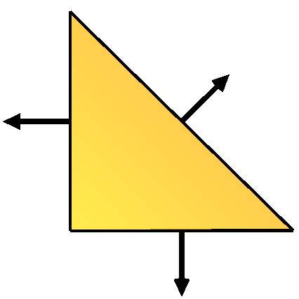
(a) $\mathrm{RT}_{0}$

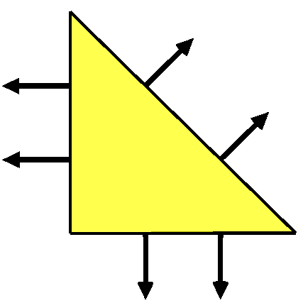
(b) $\mathrm{BDM}_{1}$

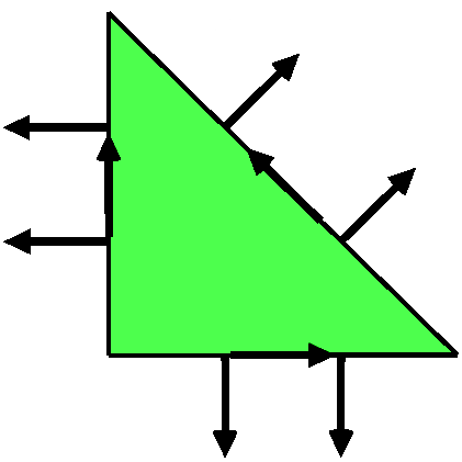
(c) $\mathrm{BDFM}_{1}$

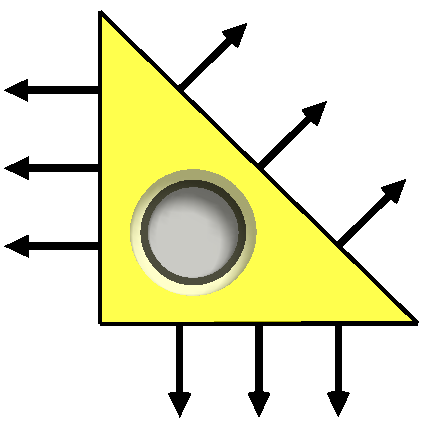
(d) $\mathrm{BDM}_{2}$

Figure 1: The degrees of freedom for the different velocity function spaces. $\mathrm{RT}_{0}$ requires the zeroth moment of the normal component on edges or, equivalently, point evaluation of the normal component at the midpoint of each edge. $\mathrm{BDM}_{1}$ requires zeroth and first moments on edges, or two point evaluations. $\mathrm{BDFM}_{1}$ additionally requires the zeroth moment of tangential velocity on each edge, local to each cell, since the tangential velocity can be discontinuous between neighbouring cells. Finally, $\mathrm{BDM}_{2}$ requires three pointwise evaluations of normal velocity on each edge, plus three additional interior moments.

It is known that $\mathrm{RT}$ spaces on triangles have a surplus of pressure degrees of freedom [DOFs] and consequently have spurious inertia-gravity modes. $\mathrm{BDM}$ spaces have a deficit of pressure DOFs and consequently have spurious Rossby modes. $\mathrm{BDFM}_{1}$ has an exact balance of velocity and pressure degrees of freedom, which is a necessary condition for the absence of spurious modes (Cotter and Shipton, 2012), hence its inclusion in our tests.

Although we will only present results for the four triples mentioned above, any member of the infinite families ${\left({\mathrm{P}}_{n},\mathrm{RT}_{n-1},{\mathrm{P}}_{n-1}^{\mathrm{DG}}\right)}$ and ${\left({\mathrm{P}}_{n+1},\mathrm{BDM}_{n},{\mathrm{P}}_{n-1}^{\mathrm{DG}}\right)}$ could be used, and three of our four triples are from said families (${\mathrm{P}}_{0}^{\mathrm{DG}}$ and ${\mathrm{P}}_{0}$ are synonymous). Also, as discussed in the previous section, the choice of the velocity space $\mathrm{S}$ determines $\mathrm{V}$ and $\mathrm{E}$. Therefore, from here onwards, we will only refer to the velocity space used – $\mathrm{RT}_{0}$, $\mathrm{BDM}_{1}$, $\mathrm{BDFM}_{1}$ or $\mathrm{BDM}_{2}$ – when presenting our results.

To emulate a boundary-free domain, we used $[0,1]^{2}$ equipped with periodic boundary conditions throughout. All lengths are therefore non-dimensional. We used both regular and unstructured meshes; examples are given in Figure 2. The regular meshes are available in FEniCS by default. The unstructured meshes were generated in gmsh (Geuzaine and Remacle, 2009) with ‘target element size’ $\frac{1}{8}$, $\frac{1}{12}$, $\frac{1}{16}$, $\frac{1}{24}$ and $\frac{1}{32}$. This gave grids with 160, 416, 736, 1488 and 2744 triangles respectively. For the unstructured grids, we have plotted errors against the total number of DOFs. For $\mathrm{RT}_{0}$, there are 1.5 global velocity DOFs and 1 height DOF per triangle. For $\mathrm{BDM}_{1}$, the corresponding numbers are 3 and 1. For $\mathrm{BDFM}_{1}$, 6 and 3; for $\mathrm{BDM}_{2}$, 7.5 and 3.

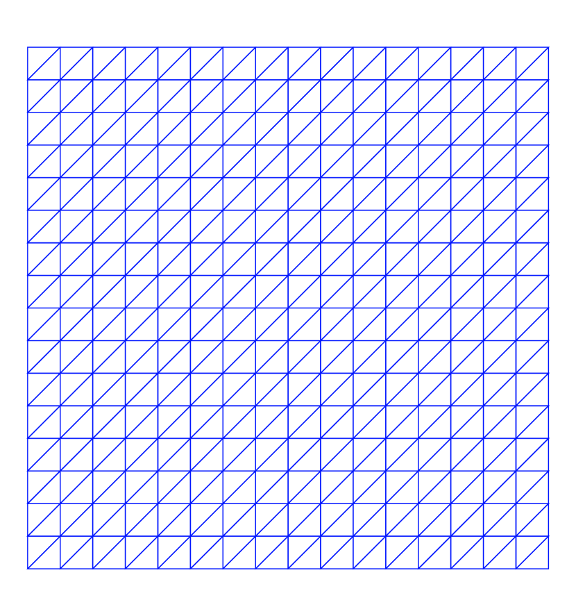
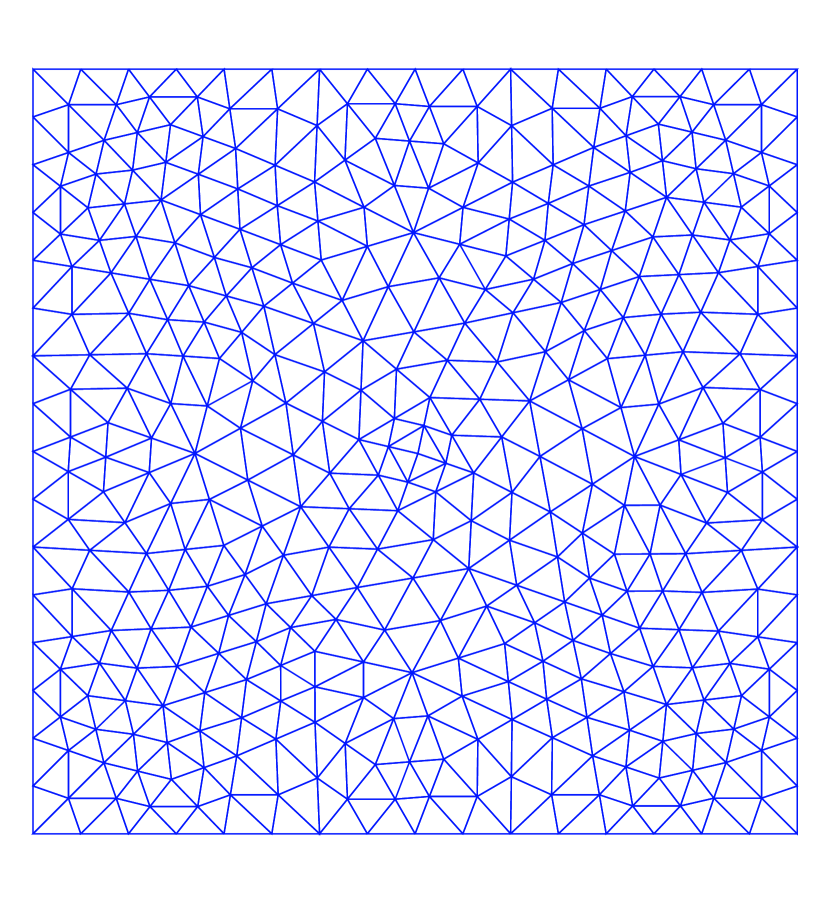
Figure 2: Examples of regular and unstructured meshes.

We will begin by examining the original, unstabilised scheme, and verifying that the discrete conservation results indeed hold. We will then look at the effects of the APVM stabilisation.

4.1 Balanced state

We performed a convergence test to verify that our implementation is correct. Here, we restricted ourselves to solutions of the form ${\mathbf{u}=(u(y),0)}$, ${h=h(y)}$, and $f$ constant. Then the shallow-water equations reduce to

$$\frac{\partial{u}}{\partial{t}}=0,\qquad fu=-g\frac{\partial{h}}{\partial{y}},\qquad\frac{\partial h}{\partial t}=0\ .$$ (4.1)

This is a simple example of geostrophic balance, in which the Coriolis force balances the pressure term exactly, and the advection terms vanish.

For our tests we made the particular choice

$$\begin{split}u&=\sin(4\pi y)\ ,\\ h&=10+\frac{1}{4\pi}\frac{f}{g}\cos(4\pi y)\ ,\end{split}$$ (4.2)

where we have nondimensionalised time accordingly (recall that the domain had non-dimensional width 1). We will take ${f=10.0}$ and ${g=10.0}$, with the appropriate nondimensionalisations, giving a Rossby number ${Ro\equiv\frac{UL}{f}\simeq 0.1}$ and a Burger number ${B\equiv\frac{gH}{f^{2}L^{2}}\simeq 1}$. We used RK4 timestepping with ${\Delta t=0.0005}$ until ${t=1}$, a regime in which timestepping error is far smaller than spatial discretisation error.

The $L^{2}$ norms of ${\mathbf{u}_{\textrm{final}}-\mathbf{u}_{\textrm{initial}}}$ and ${h_{\textrm{final}}-h_{\textrm{initial}}}$ are shown in figures 3 and 4 for a structured mesh, and figure 5 for an unstructured mesh. We see at least second-order convergence for all the schemes. This is an order more than we would naively expect for $\mathrm{RT}_{0}$. $\mathrm{BDFM}_{1}$ and $\mathrm{BDM}_{2}$ both have quadratic representations of $q$ which may explain the third order convergence, which is especially noticeable on the unstructured grid.

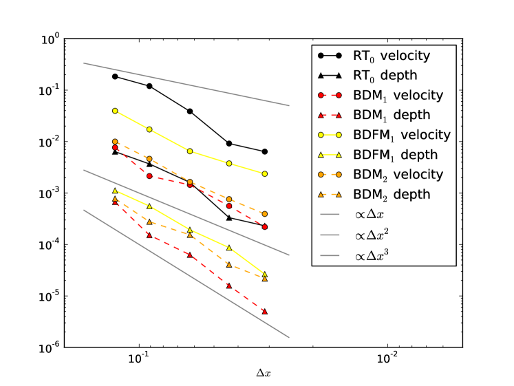
Figure 3: $L^{2}$ norms of relative velocity and height errors when simulating the balanced state described in section 4.1, with the unstabilised scheme, on a regular mesh. Error plotted against $\Delta x$.

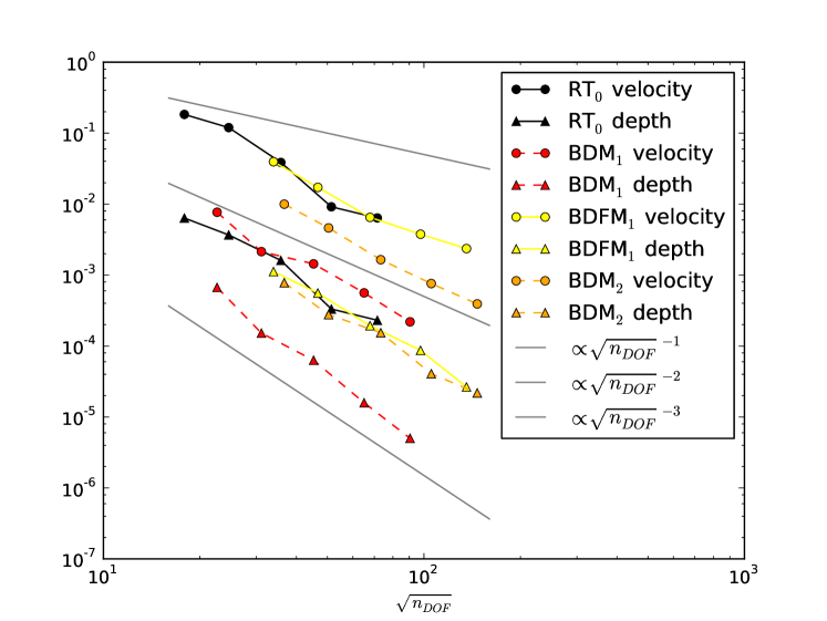
Figure 4: $L^{2}$ norms of relative velocity and height errors when simulating the balanced state described in section 4.1, with the unstabilised scheme, on a regular mesh. Error plotted against the square root of $n_{DOF}$.

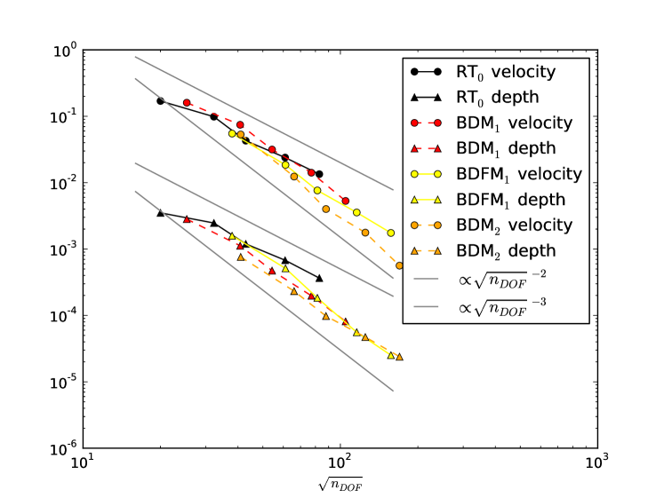
Figure 5: $L^{2}$ norms of relative velocity and height errors when simulating the balanced state described in section 4.1, with the unstabilised scheme, on an unstructured mesh.

4.2 Energy and Enstrophy conservation

To demonstrate energy and enstrophy conservation, we took an arbitrary initial condition and parameters ${f=5.0}$, ${g=5.0}$. The system was simulated with RK4 timestepping for a range of $\Delta t$ until ${t=1.001}$. Although the spatial discretisation conserves energy and enstrophy, the temporal discretisation does not. We expect to see at most fourth-order errors in the conservation of energy and enstrophy, with changing $\Delta t$, as the discrete-time numerical solutions approach the continuous-time, discrete-space solutions. We used the initial condition

$$\begin{split}\mathbf{u}&=(0,v(x))=(0,\sin(2\pi x))\\ h&=h(y)=1+\frac{1}{4\pi}\frac{f}{g}\sin(4\pi y)\end{split}$$ (4.3)

The relative changes in energy and enstrophy between the initial and final states are shown in figures 6 and 7. The former is for a regular mesh with ${\Delta x=\frac{1}{16}}$, the latter for an unstructured mesh with 736 triangles. In both cases, the enstrophy change is fourth-order in $\Delta t$. The energy change is fifth-order in $\Delta t$; we believe that this is due to additional cancellations in the equation for energy evolution.

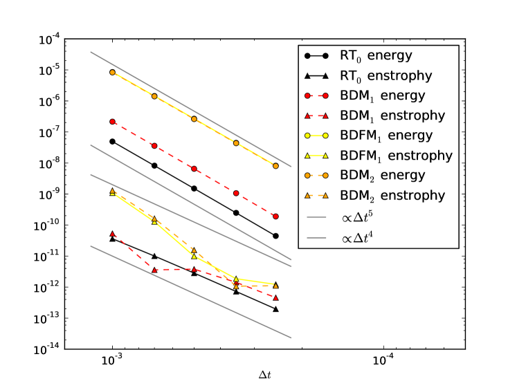
Figure 6: Relative energy and enstrophy errors when the initial condition given in section 4.2 is simulated, with the unstabilised scheme, on a regular mesh with ${\Delta x=\frac{1}{16}}$.

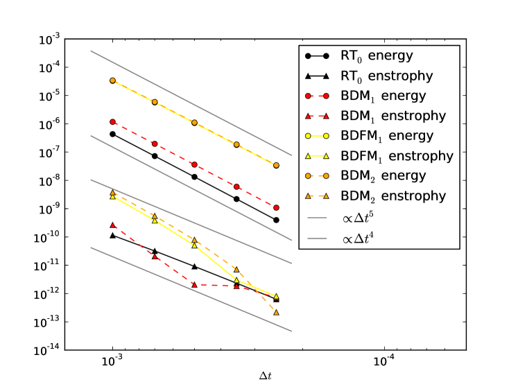
Figure 7: Relative energy and enstrophy errors when the initial condition given in section 4.2 is simulated, with the unstabilised scheme, on an unstructured mesh with 736 triangles.

4.3 Stabilised scheme

We repeated the balanced state convergence test for the scheme stabilised by the APVM. The $L^{2}$ norms of ${\mathbf{u}_{\textrm{final}}-\mathbf{u}_{\textrm{initial}}}$ and ${h_{\textrm{final}}-h_{\textrm{initial}}}$ are shown in figures 8 and 9 for a regular and unstructured grid, respectively. Note that the numerical values from the stabilised scheme are almost identical to the unstabilised scheme, to within a couple of percent.

Figure 8: $L^{2}$ norms of relative velocity and height errors when simulating the balanced state described in section 4.1, with the stabilised scheme, on a regular mesh.

Figure 9: $L^{2}$ norms of relative velocity and height errors when simulating the balanced state described in section 4.1, with the stabilised scheme, on an unstructured mesh.

We tested for energy conservation using the same initial conditions as were used in section 4.2, on the same unstructured grid, and examined the enstrophy loss. These are shown in figures 10 and 11 respectively. As before, the energy change appears to be at least fourth-order in $\Delta t$ while, as expected, enstrophy is now dissipated.

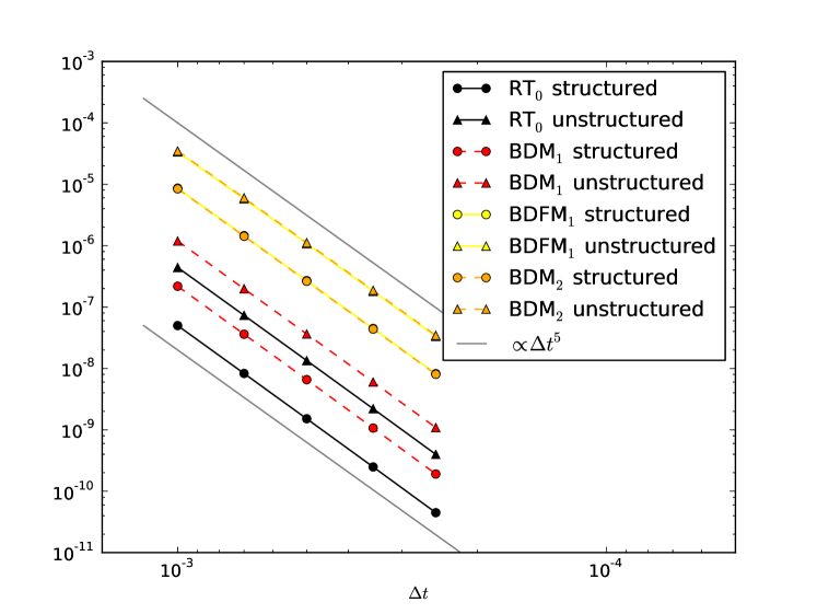
Figure 10: Relative energy error using the Anticipated Potential Vorticity Method to stabilise the proposed scheme. As before, it appears to be fifth-order in $\Delta t$, consistent with the use of RK4 timestepping.

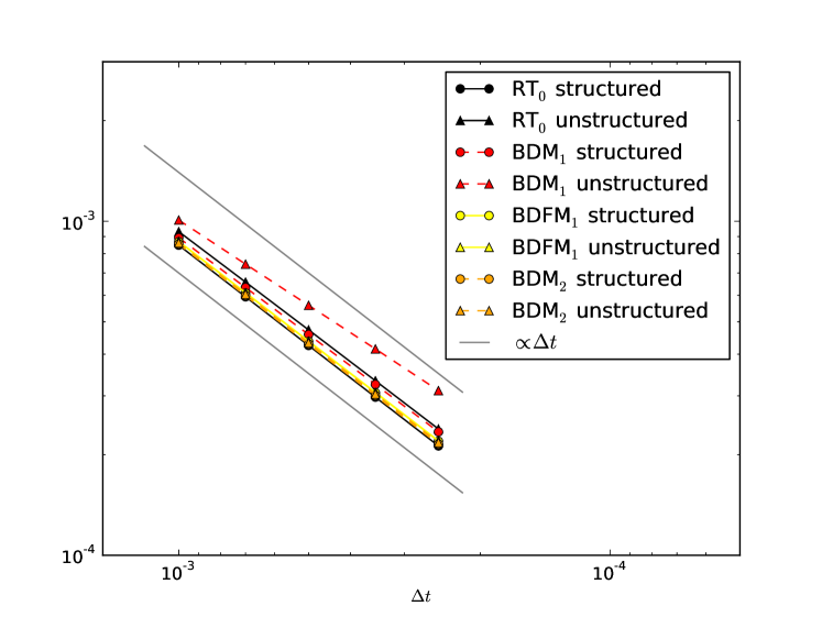
Figure 11: Relative enstrophy change using the Anticipated Potential Vorticity Method to stabilise the proposed scheme. As the APVM erodes enstrophy, we no longer see fourth-order convergence. First-order convergence is seen, since we took ${\tau=\frac{\Delta t}{2}}$

Finally, in figures 13 and 14, we show the evolution of a ‘merging vortex’ problem, in a quasi-geostrophic parameter regime, in order to visually compare the stabilised and unstabilised schemes. The initial condition for the velocity field is derived from a streamfunction: a superposition of two radially-symmetric Gaussians with different centrepoints. The initial condition for the depth field is chosen to satisfy linear geostrophic balance. The $\mathrm{BDM}_{1}$ function space was used for these examples. Enstrophy evolution is shown in figure 12. This example demonstrates the ability of the APVM to dissipate enstrophy on an unstructured mesh in this framework whilst preserving energy (up to timestepping error). The $L_{2}$ norm of the linear geostrophic imbalance $f\mathbf{u}^{\perp}+g\nabla h$ was calculated at each timestep, and the differences between with and without APVM were orders of magnitude smaller than the variation in the imbalance in either case, which in itself was very small, demonstrating that APVM does not generate fast inertia-gravity waves.

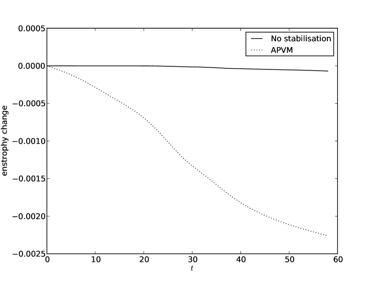
Figure 12: Evolution of total enstrophy in the ‘merging vortex’ problem. The stabilised scheme loses a macroscopic amount of enstrophy, while the unstabilised scheme only loses enstrophy due to numerical error.

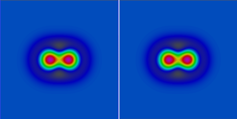
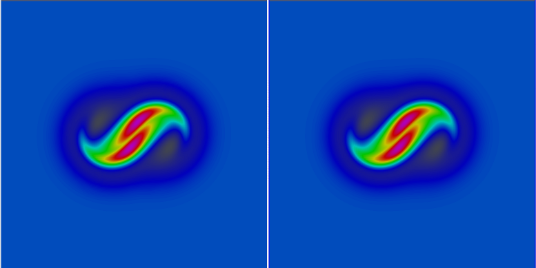
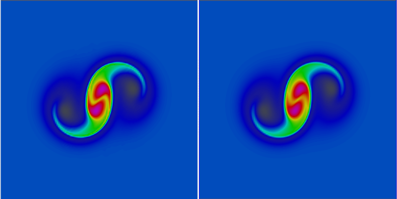
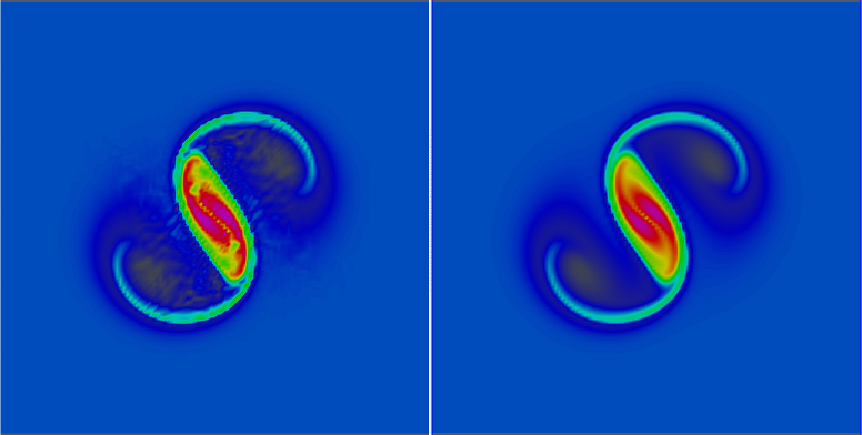
Figure 13: Evolution of merging vortices. The potential vorticity $q$ is shown, with the stabilised scheme on the right. By the fourth pair of images, spurious oscillations are visible when the unstabilised scheme is used. The plots above correspond to $t$ = 0, 8, 16, 24.

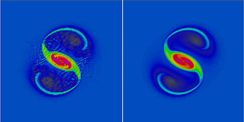
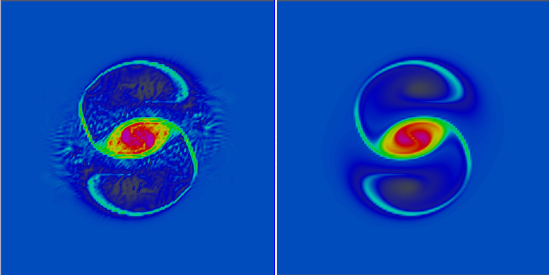
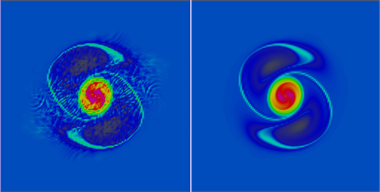
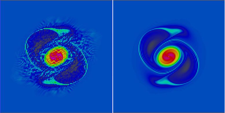
Figure 14: Evolution of merging vortices. The potential vorticity $q$ is shown, with the stabilised scheme on the right. Spurious oscillations are clearly visible when the unstabilised scheme is used. The plots above correspond to $t$ = 32, 40, 48, 56.

5 Conclusion

In this paper, we introduced a discretisation of the nonlinear shallow-water equations that extends the energy- and enstrophy-conserving formulation of Arakawa and Lamb (1981), and the energy-conserving, enstrophy-dissipating formulation of Arakawa and Hsu (1990), to the mixed finite element approach advocated in Cotter and Shipton (2012). The extension is obtained by replacing the discrete differential operators defined on the C-grid by div and curl operators that map between different finite element spaces. Given these operators, the steps are then identical to the C-grid approach: a discrete volume flux is obtained, a potential vorticity is diagnosed and the discrete volume flux is used to create a discrete potential vorticity flux. This flux is then used in the vector-invariant form of the equation for $\mathbf{u}$. The energy- and enstrophy-conservation arises from a discrete Poisson bracket structure, to be discussed in the Appendix. The convergence and energy/enstrophy properties of the scheme were demonstrated using numerical examples.

In ongoing work, we are developing semi-implicit versions of this discretisation approach, as well as extending it to curved elements for meshing the sphere, with the aim of prototyping horizontal discretisations for the UK GungHo Dynamical Core project. We are also exploring the replacement of (3.12) with an upwind discontinuous Galerkin scheme (which would dissipate potential energy at the gridscale) to avoid solution of a global mass matrix, and the use of explicit Taylor-Galerkin schemes to extend the time accuracy of the implied PV equation whilst maintaining stability. We are also investigating the extension of the finite element framework to three-dimensional flows.

Appendix A Almost-Poisson structure of the spatial discretisation

In this section, we briefly discuss the Poisson structure underlying our spatial discretisation, which will explain the origin of the conservation of energy and enstrophy. For any functional ${F(\mathbf{u},h)}$, ${F\colon\mathrm{S}\times\mathrm{V}\to\mathbb{R}}$, we calculate

$$\frac{\mathrm{d}F}{\mathrm{d}t} =\left\langle\frac{\delta F}{\delta\mathbf{u}},\mathbf{u}_{t}\right\rangle+\left\langle\frac{\delta F}{\delta h},h_{t}\right\rangle\ ,$$ (A.1)

where ${\frac{\delta F}{\delta\mathbf{u}}\in S}$ satisfies

$$\left\langle\frac{\delta F}{\delta\mathbf{u}},\mathbf{w}\right\rangle=\lim_{\varepsilon\to 0}\frac{1}{\varepsilon}\left(F(\mathbf{u}+\varepsilon\mathbf{w},h)-F(\mathbf{u},h)\right)\ ,\quad\forall\mathbf{w}\in\mathrm{S}\ ,$$ (A.2)

and similarly ${\frac{\delta F}{\delta h}\in V}$ satisfies

$$\left\langle\frac{\delta F}{\delta h},\phi\right\rangle=\lim_{\varepsilon\to 0}\frac{1}{\varepsilon}\left(F(\mathbf{u},h+\varepsilon\phi)-F(\mathbf{u},h)\right)\ ,\quad\forall\phi\in\mathrm{V}\ .$$ (A.3)

Proceeding with the calculation, we obtain

$$\frac{\mathrm{d}F}{\mathrm{d}t} =\left\langle\frac{\delta F}{\delta\mathbf{u}},-q\mathbf{F}^{\perp}\right\rangle+\left\langle\nabla\cdot\frac{\delta F}{\delta\mathbf{u}},gh+\frac{|\mathbf{u}|^{2}}{2}\right\rangle-\left\langle\frac{\delta F}{\delta h},\nabla\cdot\mathbf{F}\right\rangle$$

$$=\left\langle\frac{\delta F}{\delta\mathbf{u}},-q\frac{\delta H}{\delta\mathbf{u}}^{\perp}\right\rangle+\left\langle\nabla\cdot\frac{\delta F}{\delta\mathbf{u}},\frac{\delta H}{\delta h}\right\rangle-\left\langle\frac{\delta F}{\delta h},\nabla\cdot\frac{\delta H}{\delta\mathbf{u}}\right\rangle:=\left\{F,H\right\}\ ,$$ (A.4)

where $H$ is the Hamiltonian defined by

$$H=\frac{1}{2}\left\langle\mathbf{u},h\mathbf{u}\right\rangle+\frac{1}{2}\left\langle gh,h\right\rangle\ .$$ (A.5)

Equation (A.4) defines a bilinear bracket for functions ${\mathrm{S}\times\mathrm{V}\to\mathbb{R}}$, which is antisymmetric by inspection. This bracket is the restriction to finite elements of a standard Poisson bracket for shallow-water dynamics. Since we have not proven the Jacobi identity for the finite element bracket, we only know that it is an almost-Poisson bracket.

We obtain energy conservation immediately, since ${\dot{H}=\{H,H\}=0}$. It turns out that enstrophy ${C=\langle q,qh\rangle}$ is a Casimir for this bracket, since

$$\delta C =\left\langle 2\delta q,qh\right\rangle+\left\langle q^{2},\delta h\right\rangle$$

$$=\left\langle 2\nabla^{\perp}\delta q,\mathbf{u}\right\rangle+\left\langle 2\delta q,f\right\rangle+\left\langle q^{2},\delta h\right\rangle\ ,$$ (A.6)

and therefore ${\frac{\delta C}{\delta\mathbf{u}}=-2\nabla^{\perp}q}$ (since ${\nabla^{\perp}q\in\mathrm{S}}$), and

$$\left\langle\frac{\delta C}{\delta h},\delta h\right\rangle=\left\langle q^{2},\delta h\right\rangle\ .\quad\forall\delta h\in V.$$ (A.7)

Hence, for any functional $G$,

$$\{C,G\} =\left\langle 2q\nabla^{\perp}q,\frac{\delta G}{\delta\mathbf{u}}^{\perp}\right\rangle+\left\langle\underbrace{\nabla\cdot-2\nabla^{\perp}q}_{=0},\frac{\delta G}{\delta h}\right\rangle-\left\langle q^{2},\nabla\cdot\frac{\delta G}{\delta\mathbf{u}}\right\rangle$$ (A.8)

$$=\left\langle\nabla q^{2},\frac{\delta G}{\delta\mathbf{u}}\right\rangle-\left\langle q^{2},\nabla\cdot\frac{\delta G}{\delta\mathbf{u}}\right\rangle$$ (A.9)

$$=0\ ,$$

where we may integrate by parts in the last line since ${q\in\mathrm{E}}$ and ${\mathbf{u}\in\mathrm{S}}$. $C$ vanishes in the bracket with any other functional and therefore is a Casimir, i.e. a conserved quantity for any choice of $H$. Unfortunately, there are no known Poisson time integrators for this type of nonlinear bracket; in particular, the implicit midpoint rule is not a Poisson integrator for this bracket.

References

- Arakawa (1966) Akio Arakawa. Computational design for long-term numerical integration of the equations of fluid motion: Two-dimensional incompressible flow. Part I. Journal of Computational Physics, 1(1):119–143, 1966. doi: 10.1016/0021-9991(66)90015-5.
- Arakawa and Hsu (1990) Akio Arakawa and Yueh-Jiuan G. Hsu. Energy conserving and potential-enstrophy dissipating schemes for the shallow water equations. Monthly Weather Review, 118(10):1960–1969, 1990. doi: 10.1175/1520-0493(1990)1181960:ECAPED2.0.CO;2.
- Arakawa and Lamb (1977) Akio Arakawa and Vivian R. Lamb. Computational design of the basic dynamical processes of the UCLA general circulation model. In General Circulation Models of the Atmosphere, volume 17 of Methods in Computational Physics: Advances in Research and Applications, pages 173–265. Elsevier, 1977. doi: 10.1016/B978-0-12-460817-7.50009-4.
- Arakawa and Lamb (1981) Akio Arakawa and Vivian R. Lamb. A potential enstrophy and energy conserving scheme for the shallow water equations. Monthly Weather Review, 109(1):18–36, 1981. doi: 10.1175/1520-0493(1981)1090018:APEAEC2.0.CO;2.
- Arnold et al. (2006) Douglas N. Arnold, Richard S. Falk, and Ragnar Winther. Finite element exterior calculus, homological techniques, and applications. Acta Numerica, 15:1–155, 2006. doi: 10.1017/S0962492906210018.
- Arnold et al. (2010) Douglas N. Arnold, Richard S. Falk, and Ragnar Winther. Finite element exterior calculus: from Hodge theory to numerical stability. Bulletin (New Series) of the American Mathematical Society, 47(2):281–354, 2010. doi: 10.1090/S0273-0979-10-01278-4.
- Bonaventura and Ringler (2005) Luca Bonaventura and Todd Ringler. Analysis of discrete shallow-water models on geodesic Delaunay grids with C-type staggering. Monthly Weather Review, 133(8):2351–2373, 2005. doi: 10.1175/MWR2986.1.
- Brezzi and Fortin (1991) Franco Brezzi and Michel Fortin. Mixed and Hybrid Finite Element Methods. Springer Series in Computational Mathematics. Springer-Verlag, 1991. ISBN 0-387-97582-9.
- Brezzi et al. (1985) Franco Brezzi, Jim Douglas, Jr., and L. D. Marini. Two families of mixed finite elements for second order elliptic problems. Numerische Mathematik, 47(2):217–235, 1985. doi: 10.1007/BF01389710.
- Brooks and Hughes (1982) AN Brooks and Thomas JR Hughes. Streamline upwind/Petrov–Galerkin formulations for convection dominated flows with particular emphasis on the incompressible Navier–Stokes equations. Computer Methods in Applied Mechanics and Engineering, 32(1–3):199–259, 1982. doi: 10.1016/0045-7825(82)90071-8.
- Comblen et al. (2010) Richard Comblen, Jonathan Lambrechts, Jean-François Remacle, and Vincent Legat. Practical evaluation of five partly discontinuous finite element pairs for the non-conservative shallow water equations. International Journal for Numerical Methods in Fluids, 63(6):701–724, 2010. doi: 10.1002/fld.2094.
- Cotter and Ham (2011) C. J. Cotter and D. A. Ham. Numerical wave propagation for the triangular – finite element pair. Journal of Computational Physics, 230(8):2806–2820, 2011. doi: 10.1016/j.jcp.2010.12.024.
- Cotter and Shipton (2012) C. J. Cotter and J. Shipton. Mixed finite elements for numerical weather prediction. Journal of Computational Physics, 231:7076–7091, 2012. doi: 10.1016/j.jcp.2012.05.020.
- Danilov (2010) Sergey Danilov. On utility of triangular C-grid type discretization for numerical modeling of large-scale ocean flows. Ocean Dynamics, 60(6):1361–1369, 2010. doi: 10.1007/s10236-010-0339-6.
- Danilov et al. (2008) Sergey Danilov, Qiang Wang, Martin Losch, Dmitry Sidorenko, and Jens Schröter. Modeling ocean circulation on unstructured meshes: comparison of two horizontal discretizations. Ocean Dynamics, 58(5-6):365–374, 2008. doi: 10.1007/s10236-008-0138-5.
- Donea (1984) Jean Donea. A Taylor–Galerkin method for convective transport problems. International Journal for Numerical Methods in Engineering, 20(1):101–119, 1984. doi: 10.1002/nme.1620200108.
- Gassmann (2011) Almut Gassmann. Inspection of hexagonal and triangular c-grid discretizations of the shallow water equations. Journal of Computational Physics, 230(7):2706–2721, 2011. doi: 10.1016/j.jcp.2011.01.014.
- Gassmann and Herzog (2008) Almut Gassmann and Hans-Joachim Herzog. Towards a consistent numerical compressible non-hydrostatic model using generalized Hamiltonian tools. Quarterly Journal of the Royal Meteorological Society, 134(635):1597–1613, 2008. doi: 10.1002/qj.297.
- Geuzaine and Remacle (2009) Christophe Geuzaine and Jean-François Remacle. Gmsh: A 3-D finite element mesh generator with built-in pre-and post-processing facilities. International Journal for Numerical Methods in Engineering, 79(11):1309–1331, 2009. doi: 10.1002/nme.2579.
- Gresho and Sani (1998) Philip M Gresho and Robert L Sani. Incompressible flow and the finite element method. Volume 1: Advection-diffusion and isothermal laminar flow. John Wiley and Sons, 1998. ISBN 0-471-49249-3.
- Hallberg and Rhines (1996) Robert Hallberg and Peter Rhines. Buoyancy-driven circulation in an ocean basin with isopycnals intersecting the sloping boundary. Journal of Physical Oceanography, 26(6):913–940, 1996. doi: 10.1175/1520-0485(1996)0260913:BDCIAO2.0.CO;2.
- Hyman and Shashkov (1997) J. M. Hyman and M. Shashkov. Natural discretizations for the divergence, gradient, and curl on logically rectangular grids. Computers & Mathematics with Applications, 33(4):81–104, 1997. doi: 10.1016/S0898-1221(97)00009-6.
- Le Roux et al. (2009) D. Y. Le Roux, E. Hanert, V. Rostand, and B. Pouliot. Impact of mass lumping on gravity and rossby waves in 2D finite-element shallow-water models. International Journal for Numerical Methods in Fluids, 59(7):767–790, 2009. doi: 10.1002/fld.1837.
- Le Roux (2005) Daniel Y. Le Roux. Dispersion relation analysis of the finite-element pair in shallow-water models. SIAM Journal on Scientific Computing, 27(2):394–414, 2005. doi: 10.1137/030602435.
- Le Roux (2012) Daniel Y Le Roux. Spurious inertial oscillations in shallow-water models. Journal of Computational Physics, 231(6):7959–7987, 2012. doi: 10.1016/j.jcp.2012.04.052.
- Le Roux and Pouliot (2008) Daniel Y. Le Roux and Benoit Pouliot. Analysis of numerically induced oscillations in two-dimensional finite-element shallow-water models part II: Free planetary waves. SIAM Journal on Scientific Computing, 30(4):1971–1991, 2008. doi: 10.1137/070697872.
- Le Roux et al. (2007) Daniel Y. Le Roux, Virgile Rostand, and Benoit Pouliot. Analysis of numerically induced oscillations in 2D finite-element shallow-water models part I: Inertia-gravity waves. SIAM Journal on Scientific Computing, 29(1):331–360, 2007. doi: 10.1137/060650106.
- Logg et al. (2012) Anders Logg, Kent-Andre Mardal, and Garth N. Wells. Automated Solution of Differential Equations by the Finite Element Method. Springer, 2012. ISBN 978-3-642-23098-1. doi: 10.1007/978-3-642-23099-8.
- Raviart and Thomas (1977) P. A. Raviart and J. M. Thomas. A mixed finite element method for 2-nd order elliptic problems. In Mathematical aspects of finite element methods, pages 292–315. Springer, 1977. doi: 10.1007/BFb0064470.
- Ringler et al. (2010) T. D. Ringler, J. Thuburn, J. B. Klemp, and W. C. Skamarock. A unified approach to energy conservation and potential vorticity dynamics for arbitrarily-structured C-grids. Journal of Computational Physics, 229(9):3065–3090, 2010. doi: 10.1016/j.jcp.2009.12.007.
- Rognes et al. (2009) Marie E Rognes, Robert C Kirby, and Anders Logg. Efficient assembly of H(div) and H(curl) conforming finite elements. SIAM Journal on Scientific Computing, 31(6):4130–4151, 2009. doi: 10.1137/08073901X.
- Rostand and Le Roux (2008) V Rostand and DY Le Roux. Raviart–Thomas and Brezzi–Douglas–Marini finite-element approximations of the shallow-water equations. International Journal for Numerical Methods in Fluids, 57(8):951–976, 2008. doi: 10.1002/fld.1668.
- Sadourny (1975) Robert Sadourny. The dynamics of finite-difference models of the shallow-water equations. Journal of the Atmospheric Sciences, 32(4):680–689, 1975. doi: 10.1175/1520-0469(1975)0320680:TDOFDM2.0.CO;2.
- Sadourny and Basdevant (1985) Robert Sadourny and Claude Basdevant. Parameterization of subgrid scale barotropic and baroclinic eddies in quasi-geostrophic models: Anticipated potential vorticity method. Journal of the Atmospheric Sciences, 42(13):1353–1363, 1985. doi: 10.1175/1520-0469(1985)0421353:POSSBA2.0.CO;2.
- Salmon (2005) Rick Salmon. A general method for conserving quantities related to potential vorticity in numerical models. Nonlinearity, 18(5):R1, 2005.
- Salmon (2007) Rick Salmon. A general method for conserving energy and potential enstrophy in shallow-water models. Journal of the Atmospheric Sciences, 64(2):515–531, 2007. doi: 10.1175/JAS3837.1.
- Sommer and Névir (2009) Matthias Sommer and Peter Névir. A conservative scheme for the shallow-water system on a staggered geodesic grid based on a Nambu representation. Quarterly Journal of the Royal Meteorological Society, 135(639):485–494, 2009. doi: 10.1002/qj.368.
- Staniforth and Thuburn (2012) Andrew Staniforth and John Thuburn. Horizontal grids for global weather and climate prediction models: a review. Quarterly Journal of the Royal Meteorological Society, 138(662):1–26, 2012. doi: 10.1002/qj.958.
- Staniforth et al. (2012) Andrew Staniforth, Thomas Melvin, and Colin Cotter. Analysis of a mixed finite-element pair proposed for an atmospheric dynamical core. Quarterly Journal of the Royal Meteorological Society, 2012. doi: 10.1002/qj.2028.
- Thuburn (2008) J. Thuburn. Numerical wave propagation on the hexagonal C-grid. Journal of Computational Physics, 227(11):5836–5858, 2008. doi: 10.1016/j.jcp.2008.02.010.
- Thuburn and Cotter (2012) J. Thuburn and C. J. Cotter. A framework for mimetic discretization of the rotating shallow-water equations on arbitrary polygonal grids. SIAM Journal on Scientific Computing, 34(3):B203–B225, 2012. doi: 10.1137/110850293.
- Thuburn et al. (2009) J. Thuburn, T. D. Ringler, W. C. Skamarock, and J. B. Klemp. Numerical representation of geostrophic modes on arbitrarily structured C-grids. Journal of Computational Physics, 228(22):8321–8335, 2009. doi: 10.1016/j.jcp.2009.08.006.
- Wathen (1987) A. J. Wathen. Realistic eigenvalue bounds for the Galerkin mass matrix. IMA Journal of Numerical Analysis, 7(4):449–457, 1987. doi: 10.1093/imanum/7.4.449.