Evolution of Thermally Pulsing Asymptotic Giant Branch Stars I. The COLIBRI Code

Abstract

We present the COLIBRI code for computing the evolution of stars along the TP-AGB phase. Compared to purely synthetic TP-AGB codes, COLIBRI relaxes a significant part of their analytic formalism in favour of a detailed physics applied to a complete envelope model, in which the stellar structure equations are integrated from the atmosphere down to the bottom of the hydrogen-burning shell. This allows to predict self-consistently: (i) the effective temperature, and more generally the convective envelope and atmosphere structures, correctly coupled to the changes in the surface chemical abundances and gas opacities; (ii) the conditions under which sphericity effects may significantly affect the atmospheres of giant stars; (iii) the core mass-luminosity relation and its possible break-down due to the occurrence of hot bottom burning (HBB) in the most massive AGB stars, by taking properly into account the nuclear energy generation in the H-burning shell and in the deepest layers of the convective envelope; (iv) the HBB nucleosynthesis via the solution of a complete nuclear network (including the pp chains, and the CNO, NeNa, MgAl cycles) coupled to a diffusive description of mixing, suitable to follow also the synthesis of ⁷Li via the Cameron-Fowler beryllium transport mechanism; (v) the intershell abundances left by each thermal pulse via the solution of a complete nuclear network applied to a simple model of the pulse-driven convective zone; (vi) the onset and quenching of the third dredge-up, with a temperature criterion that is applied, at each thermal pulse, to the result of envelope integrations at the stage of the post-flash luminosity peak.

At the same time COLIBRI pioneers new techniques in the treatment of the physics of stellar interiors, not yet adopted in full TP-AGB models. It is the first evolutionary code ever to use accurate on-the-fly computation of the equation of state for roughly 800 atoms, ions, molecules, and of the Rosseland mean opacities throughout the atmosphere and the deep envelope. This ensures a complete consistency, step by step, of both EoS and opacity with the evolution of the chemical abundances caused by the third dredge-up and HBB. Another distinguishing aspect of COLIBRI is its high computational speed, that allows to generate complete grids of TP-AGB models in just a few hours. This feature is absolutely necessary for calibrating the many uncertain parameters and processes that characterize the TP-AGB phase.

We illustrate the many unique features of COLIBRI by means of detailed evolutionary tracks computed for several choices of model parameters, including initial star masses, chemical abundances, nuclear reaction rates, efficiency of the third dredge-up, overshooting at the base of the pulse-driven convection zone, etc. Future papers in this series will deal with the calibration of all these and other parameters using observational data of AGB stars in the Galaxy and in nearby systems, a step that is of paramount importance for producing reliable stellar population synthesis models of galaxies up to high redshift.

1 Context and motivation

The modelling of the Thermally Pulsing Asymptotic Giant Branch (TP-AGB) stellar evolutionary phase plays a critical role in many astrophysical issues, from the chemical composition of meteorites belonging to the pre-solar nebula (e.g. Zinner et al., 2005), up to the cosmological context of galaxy evolution in the high-redshift Universe (e.g. Maraston et al., 2006). Indeed, luminous TP-AGB stars are potentially the dominant contribution to a galaxy’s flux, particularly at the red wavelengths and high redshifts that are much of the focus of modern extragalactic astronomy. In spite of its importance, the TP-AGB phase is still affected by large uncertainties which uncomfortably propagate into the field of current population synthesis models of galaxies that, for this reason, are strongly debated (e.g. Conroy, Gunn & White, 2009; Kriek et al., 2010; Zibetti et al., 2013).

As a matter of fact, the evolution along TP-AGB phase is determined in a crucial way by processes which are challenging to model from first principles: turbulent convection, stellar winds, and long-period variability. Also, these processes do not take place in a steady and smooth way during the TP-AGB evolution, but greatly vary in both character and efficiency over the single thermal pulse cycles (TPC) – the $10^{2}$ to $10^{5}$-yr long periods that go from one He-shell flash, through quiescent H-shell burning, up to the next He-flash. Moreover, the rich nucleosynthesis in the intershell convective region followed by recurrent dredge-up episodes, and the nuclear burning at the base of the convective envelope (hot-bottom burning, HBB) of the most massive TP-AGB stars ($M\ga 4\,M_{\odot}$), can dramatically change the surface abundances, and hence the envelope structure, over a timescale much shorter than a single TPC.

The result is that the modelling of the TP-AGB phase is quite difficult, time consuming, and affected by large uncertainties. Efforts to follow this phase with “full models”, which solve the time-dependent equations of stellar structure with the aid of classical 1D stellar evolution codes, are becoming increasingly successful thanks to the speeding-up of modern processors, and to the particular care devoted to the nucleosynthesis (e.g. Ventura, D’Antona & Mazzitelli, 2002; Cristallo et al., 2009; Karakas, 2010). However, full TP-AGB models still meet three fundamental difficulties.
(1) They are affected by quite subtle and nasty numerical uncertainties, that can greatly affect the predicted efficiency of convective dredge-up episodes even within the same set of models (Frost & Lattanzio, 1996; Mowlavi, 1999a).
(2) Full TP-AGB models need to resort to parametrized descriptions of crucial processes (mass loss, convection, overshoot), with theoretical formulations and “efficiency parameters” that may largely vary from study to study, so that to date no universally accepted set of prescriptions exists. This intrigued situation is well exemplified by fact that, for instance, the so-called carbon-star mystery, pointed out by Iben (1981) in the far past, is now claimed to have been solved by full TP-AGB models (Stancliffe, Izzard & Tout, 2005; Weiss & Ferguson, 2009; Cristallo et al., 2011). However, it is somewhat disturbing to recognize that the same observable, i.e. the carbon star luminosity function of carbon stars in the Large Magellanic Cloud, seems to be recovered by different full TP-AGB models in which the third dredge-up takes place with very different characteristics (in this respect, see Sect. 4.1 and Fig. 4).
(3) The range of parameters to be covered, and prescriptions to be tested, in order to obtain grids of TP-AGB models that reproduce the wide variety of observational data for AGB stars in resolved galaxies, is simply too large.

In this tricky context, a valuable contribution may be provided by the so-called “synthetic models”, in which the evolution from one thermal pulse to the next is described with analytical relations that synthesize the results of full models. Being very agile and hence suitable to explore wide ranges of parameters and prescriptions, synthetic models can help to constrain the physical domain towards which full models should converge in order to reproduce observations of TP-AGB stars (e.g. carbon star luminosity functions (CSLF), C/M ratios, H-R diagrams, etc.). For instance, following the work of Groenewegen & de Jong (1993), based on synthetic models and focussed on the CSLF in the Large Magellanic Cloud, it became clear that the third dredge-up should not only be much more efficient, but also start earlier, at fainter luminosities, than usually predicted by full TP-AGB models up to that time.

On the other hand, synthetic models are often criticised because they lack the accurate physics involved in the evolution of these stars. Moreover, they are completely subordinate to the relations fitting the results of full AGB model calculations, which severely limits their capability of exploring new evolutionary effects. A notable example is the effective temperature, for which various formulas have been proposed in the past in the usual form $T_{\rm eff}={\rm func}(L,M,Z)$, involving luminosity, stellar mass and metallicity. Unfortunately, their validity is extremely narrow as they can apply only to oxygen-rich stars (with surface C/O$<1$), hence being unable to account for the Hayashi limits of carbon stars. Moreover, these relations reflect the specific set of input physics adopted in the underlying full models, e.g. mixing-length parameter, gas opacities, equation of state, etc.

If this criticism reasonably applies to the purely analytic TP-AGB models that rely on a mere compilation of fitting formulas (e.g. Hurley, Pols & Tout, 2000; Izzard et al., 2004, 2006; Cordier et al., 2007), it is not as well suited to the class of hybrid models (e.g. Marigo, Bressan & Chiosi, 1996, 1998; Marigo et al., 1999; Marigo, 2007; Marigo & Girardi, 2007), in which the analytic formalism is complemented with numerical integrations of the stellar structure equations, carried out from the atmosphere down to the bottom of the convective envelope. In the latter case both the HBB nucleosynthesis and the basic changes in envelope structure – including effective temperature and radius – can be followed with the same richness of detail as in full models, but still in a much quicker and more versatile way.

It is not by accident that the crucial role of the surface C/O ratio and C-rich opacities in determining the evolution of TP-AGB stars was established just with the aid of these “envelope-based models” (Marigo, 2002, 2007; Marigo, Girardi & Chiosi, 2003; Marigo & Girardi, 2007). Although the same effect could have been assessed with the aid of full models, the latter were fighting with so many numerical and physical difficulties related to the occurrence of the third dredge-up, that the key aspect of the C-rich opacities was ignored, and likely forgotten, for long time in the field of AGB stellar evolution. Since Marigo (2002), molecular opacities for C-rich mixtures have been progressively adopted in full TP-AGB models (e.g. Kamath, Karakas & Wood, 2012; Ventura & Marigo, 2010, 2009; Weiss & Ferguson, 2009; Cristallo et al., 2007).

This example tells clearly that progresses in the description of the TP-AGB phase do not rely only on full models, but they can come also from other complementary approaches.

With this work we go a few steps ahead in the development of our “envelope-based TP-AGB models”. We describe a code, called COLIBRI, that implements a number of improvements which, effectively, make our models to perform much more like ”almost-full” models than ”improved synthetic” ones. Among the most relevant points we mention: i) a spherically-symmetric deep envelope model extending from the atmosphere down to the bottom of the quiescent H-burning shell, so that the classical core-mass luminosity relation (CMLR) is naturally predicted and not taken as an input prescription; ii) the first ever on-the-fly accurate calculation of molecular chemistry and Rosseland mean opacities, fully consistent with the changing surface abundances, iii) a detailed HBB nucleosynthesis coupled with a diffusive description of convection, iv) a model for the pulse-driven convection zone to predict the chemical composition of the dredged-up material, and v) improved prescriptions to determine the onset and quenching of the third dredge-up.

Of course, in the development of the COLIBRI code full TP-AGB models still play a paramount role: they are taken as a reference to check the accuracy of some basic predictions, and they are used to derive quantitative information, via fitting relations, on those aspects that the COLIBRI code cannot, by construction, address by itself like, for example, the evolution of the intershell convection zone during thermal pulses.

In any case, all these aspects are treated fulfilling two extremely important conditions: a robust numerical stability which allows to follow the TP-AGB evolution until the complete ejection of the envelope, and a high computational speed which is kept comparable to the levels that made the success of the very first synthetic TP-AGB models. In this way the COLIBRI code is a tool perfectly suitable to perform a multi-parametric, but still accurate, calibration of the TP-AGB phase, our final goal.

The plan of the paper is as follows. Section 2 presents an outline of the COLIBRI code. Section 3 describes in detail all input physics and the solution methods adopted to integrate the deep envelope model, and to predict the nucleosynthesis in the pulse-driven convective zone and during HBB. Section 4 summarises the analytic ingredients of COLIBRI. Accuracy tests of COLIBRI predictions against full stellar models are discussed in Sect. 5. The present sets of TP-AGB evolutionary tracks are introduced in Sect. 6, while the whole Sect. 7 is dedicated to illustrate several examples of possible COLIBRI calculations. Finally, Sect. 8 closes the paper giving a résumé of COLIBRI’s features, and briefly mentioning current and planned applications.

2 Overview of the COLIBRI code

The COLIBRI code computes the TP-AGB evolution from the first thermal pulse up to the complete ejection of the stellar mantle by stellar winds. While maintaining a few basic features of our original TP-AGB model developed and revised over the years (Marigo, Bressan & Chiosi, 1996, 1998; Marigo, 1998; Marigo et al., 1999; Marigo & Girardi, 2007), we have introduced substantial improvements that notably enhance the predictive power of our TP-AGB calculations. The main variables of the TP-AGB model, which are also frequently cited in the text, are operatively defined in Table 2.

COLIBRI consists of three main components, that we conveniently refer to as 1) the physics module, 2) the synthetic module, and 3) the parameter box.

The physics module involves all detailed input physics (equation of state, opacities, nuclear reactions rates) and differential equations necessary to numerically integrate a stationary deep envelope model, extending from the atmosphere down to the bottom of the H-burning shell (see Sect. 3). At each time step, the run of mass $M_{r}$, temperature $T_{r}$, pressure $P_{r}$, and luminosity $L_{r}$ is determined across the deep envelope during the quiescent interpulse periods. By adopting proper boundary conditions at the bottom of the convective envelope, we obtain the effective temperature, and the luminosity provided by the hydrogen burning shell. In this way we are able to follow consistently the occurrence of HBB in the most massive AGB stars, being responsible for the break-down of the CMLR (see Sect. 5.2), as well as a significant nucleosynthesis (see Sect. 3.5.2).

The synthetic module contains the analytic formalism of the code, which includes both fitting formulas that synthesize the results of full AGB models (e.g. the core mass-interpulse period relation, the core mass-intershell mass relation, the efficiency of the third dredge-up as a function of stellar mass and metallicity, etc.), and other auxiliary relations (e.g. mass-loss prescription, period-mass-radius relations for variable AGB stars, etc.). It is outlined in Sect. 4.

The parameters box collects all free parameters that we think need to be calibrated (e.g. minimum base temperature for the occurrence of the third dredge-up, efficiency of mass loss, dependence on mass and metallicity, overshoot at the base of the convective envelope) in order to reproduce basic observables. Since a fine calibration of the TP-AGB phase is not the primary purpose of this paper, the results presented here are obtained with a particular set of parameters, as specified in Sect. 6.2.

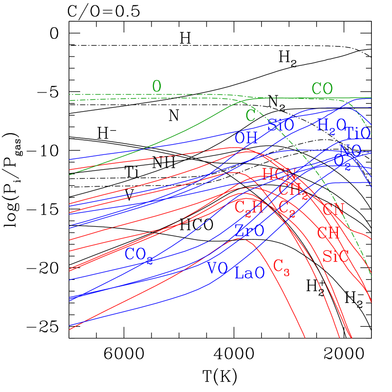
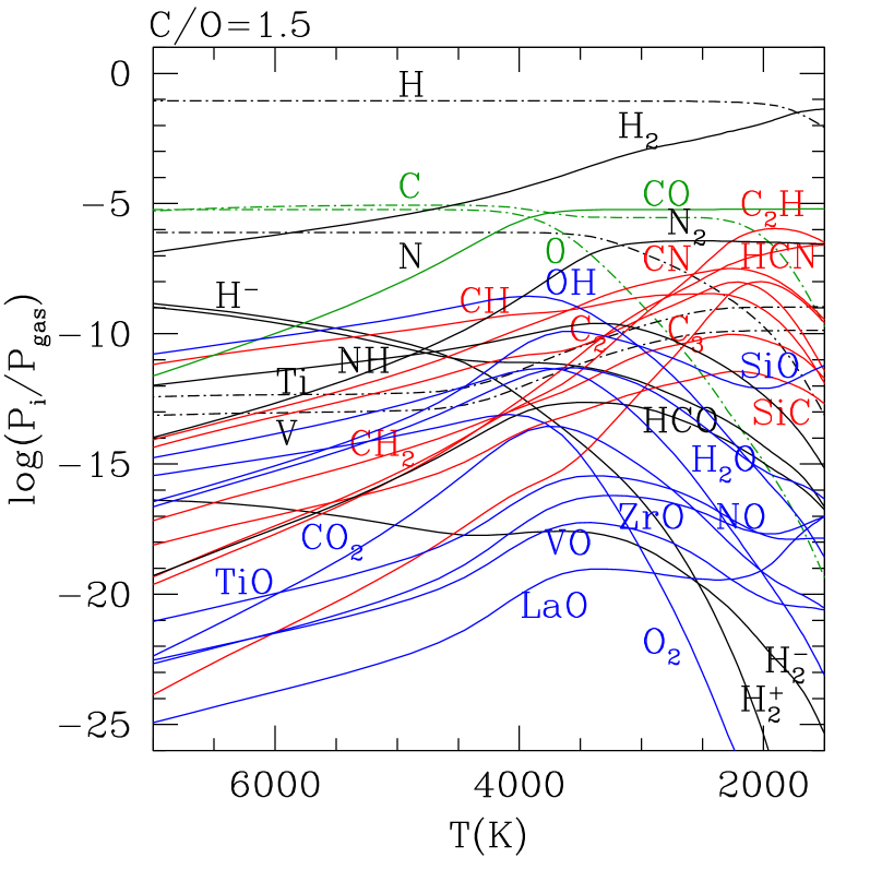
Figure 1: Partial pressures of a subset of atomic and molecular species computed with the ÆSOPUS code (Marigo & Aringer, 2009) according to the temperature-pressure stratification of a complete envelope-atmosphere model with $\log(T_{\rm eff})=3.45$, $\log(L/L_{\odot})=3.7$, $M_{\rm i}=2M_{\odot}$, and solar metallicity $Z_{\rm i}=Z_{\odot}\!\simeq\!0.0152$ following the revision by Caffau et al. (2011). Two values of the C/O ratio have been considered, i.e. C/O$=0.5$ (left-hand side panel) and C/O$=1.5$ (left-hand side panel). Note the abrupt change in the molecular equilibria of the O-bearing (blue) and C-bearing (red) molecules between the two cases, as well as the almost invariance of the abundance of the highly stable CO molecule.

These three components clearly represent a sequence of decreasing accuracy, and increasing uncertainty. While for most ingredients of the physics module we rely on detailed and well-established prescriptions, in the synthetic module we have to resort to the results of various sets of full TP-AGB models in the literature that share a general agreement, but present also unavodaible differences due to specific model details. The parameter box, instead, hides a big deal of our ignorance about basic physical processes in AGB stars. The coupling of these components, with very different degrees of accuracy, is inescapable at this point. The situation resembles the one that persists in practically all full stellar evolutionary codes to date, in which rough descriptions for convective processes – such as the mixing length theory and overshooting – are routinely adopted, and anyhow being able to produce very useful results. Although we all know that “fake physics” is being used to some extent in all these codes, it is also a matter of fact that, at some stages, these approximations have opened the way for advancing the theory of stellar evolution on other fronts. Our wish is that the same strategy can turn out to be useful also for the TP-AGB phase.

3 The physics module

3.1 Equation of state

The equation of state (EoS) for temperatures in the interval from $5\times 10^{4}$ K to $10^{8}$ K is that of a fully-ionized gas, in the way described by Girardi et al. (2000).

For temperatures in the range from $5\times 10^{4}$ K to $10^{3}$ K all relevant thermodynamic quantities and their partial derivatives (mass density, electron density, mean molecular weight, entropy, specific heats, etc.) are computed on-the-fly with the ÆSOPUS code (Marigo & Aringer, 2009). We briefly recall that ÆSOPUS solves the EoS for atoms and molecules in the gas phase, under the assumption of an ideal gas in both thermodynamic equilibrium and instantaneous chemical equilibrium. We consider the ionisation stages from I to V for all elements from C to Ni (up to VI for O and Ne), and from I to III for heavier atoms from Cu to U. Saha equations for ionisation and dissociation are solved for $\approx 800$ species, including $\approx 300$ atoms (neutral and ionised) from H to U, and $\approx 500$ molecules.

An example of the EoS calculations across the outermost layers of a TP-AGB model is given in Fig. 1, that also illustrates the dramatic change in the equilibrium molecular chemistry as the surface C/O ratio passes from ${\rm C/O}<1$, typical of M stars, to ${\rm C/O}>1$, characteristic of C stars.

3.2 Gas opacities

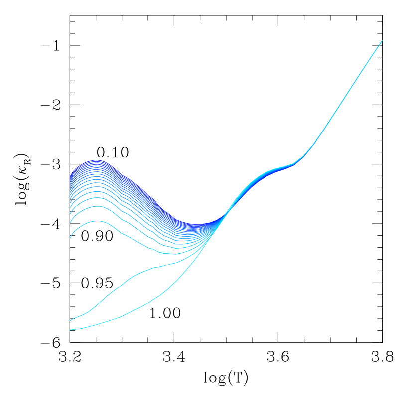
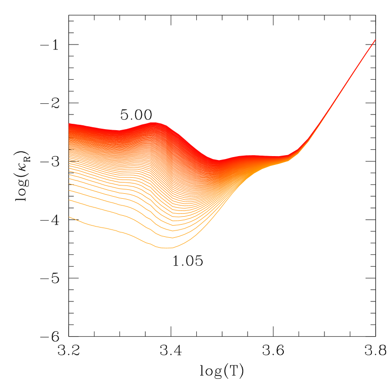
Figure 2: Rosseland mean opacities, computed with the ÆSOPUS code (Marigo & Aringer, 2009), according to the temperature-pressure stratification of a complete envelope-atmosphere model with $\log(T_{\rm eff})=3.45$, $\log(L/L_{\odot})=3.7$, $M_{\rm i}=2M_{\odot}$, and solar metallicity $Z_{\rm i}=Z_{\odot}\!\simeq\!0.0152$ according to Caffau et al. (2011). The C/O ratio is made to increase from 0.10 to 1.00 (left-hand side panel), and from 1.05 to 5.00 (right-hand side panel) in steps of 0.05.

Rosseland mean gas opacities, in the whole temperature range $8.0\leq\log T\leq 3.2$, are computed on-the-fly, i.e. contemporary with the atmospheric and envelope integrations that constitute the kernel of our TP-AGB code.

We remark that this is the first time ever that accurate opacities are computed on-the-fly, just starting from the monochromatic absorption coefficients of the opacity sources, without interpolation in pre-exiting tables of Rosseland mean opacities.

This choice is motivated by the demand of accurately describing the tight coupling of the opacity sources (mainly in the molecular regime) with the frequent and significant changes in the envelope chemical composition that characterise the TP-AGB phase. In this way we avoid the loss in accuracy that one must otherwise pay when performing multi-dimensional interpolation.

To this aim we have constructed a routine which, for any given set of chemical abundances of $92$ elements from H to U, and a specified pair of state variables (e.g. gas pressure $P_{\rm g}$ and temperature $T$), makes direct calls to one of two opacity codes, depending on the temperature:

• The Opacity Project (OP) (OP; Seaton, 2005; Badnell et al., 2005) for $4.2<\log T\leq 8.0$;

• The ÆSOPUS code (Marigo & Aringer, 2009) for $3.2\leq\log T\leq 4.2$.

The OP data provides the monochromatic opacities for several atoms (H, He, C, N, O, Na, Mg, Al, Si, S, Ar, Ca, Cr, Mn, Fe, Ni) over a wide range of values of temperature $T$ and electron density $N_{\rm e}$. We have employed the routines mixv.f and opfit.f to calculate the Rosseland mean opacities on a pre-determined grid of OP$(T,\,N_{\rm e})$ meshes and then to interpolate to any specified values of $T$ and $\rho$. Since the original OP version assumes a fixed mixture of elements (i.e. scaled-solar chemical composition), we have suitably modified the OP routines to compute the Rosseland mean for any chemical composition involving the $16$ species for which the OP monochromatic opacities are available. This is an important improvement compared to the common practice in which the chemical parameters (besides the H or He abundances) are limited to few metal abundances. For instance, the widely-used OPAL web tool (Rogers, Swenson & Iglesias, 1996) allows the on-line computation and provides the interpolating routines of Rosseland mean opacity tables with a fixed partition of metals, but for the abundances of two species (e.g. C and O), which are enhanced according to a specified grid of values. We notice that in this case, the possible depletion of a metal, due for instance to nuclear burning, cannot be considered. At variance, the OP utility gives us an important flexibility in this respect.

Suitably converted into an internal routine of our COLIBRI code, for each pair of $P_{\rm g}$ and $T$, ÆSOPUS calculates the monochromatic true absorption and scattering cross sections due to a number of continuum and discrete processes, i.e. bound-free absorption due to photoionisation, free-free absorption, Rayleigh and Thomson scattering, collision-induced absorption, atomic bound-bound absorption and molecular absorption. We note that the monochromatic cross sections for atoms (C, N, O, Na, Mg, Al, Si, S, Ar, Ca, Cr, Mn, Fe, Ni) are taken from the OP database, thus assuring a complete consistency with the high-temperature opacities. Then, after summing up all contributions, the Rosseland mean (RM) opacity is computed.

The incorporation of ÆSOPUS in the COLIBRI code allows us to follow accurately the changes in molecular opacities driven by any variation of the envelope composition, especially by the C/O ratio which plays the key role in determining the molecular chemistry (see e.g. Marigo & Aringer, 2009). The complex behaviour of the RM opacities as a function of the C/O ratio is exemplified with the aid of Fig. 2. It turns out that while the C/O ratio increases from $0.1$ to $0.9$ the opacity bump peaking at ($\log(T)\simeq 3.25-3.35$) – mostly due to H₂O – becomes more and more depressed because of the smaller availability of O atoms. Then, passing from C/O $=0.9$ up to C/O $=0.95$ the H₂O feature actually disappears and $\kappa_{\rm R}$ drastically drops by more almost two orders of magnitude. In fact, at this C/O value the chemistry enters in a transition region where most of both O and C atoms are trapped in the very stable CO molecule at the expense of the other molecular species, belonging to both the O- and C-bearing groups. At C/O $=1$ the RM opacity reaches its minimum throughout the temperature range, $3.2\la\log(T)\la 3.4$, while a sudden upturn is expected as soon as C/O slightly exceeds unity, as displayed by the curve for C/O $=1.05$ of Fig. 2 (right panel). This fact reflects the drastic change in the molecular equilibria from the O- to the C-dominated regime. Then, at increasing C/O the opacity curves move upward following a more gradual trend, which is related to the strengthening of the C-bearing molecular absorption bands.

Note, however, that the C-rich opacity does not rise linearly with C/O, but less and less steeply as the C/O ratio increases. This is mainly due to the underlying equilibrium chemistry of the most efficient absorbers, in particular of the CN and HCN molecules, whose abundances are conditioned not only by the carbon excess (C-O), but also by the availability of the N atoms (having a fixed abundance in the case under consideration). As we will see in Sect. 7.3, the non-linear dependence of the opacity on the C/O ratio impacts on the maximum extension of the Hayashi lines for C stars towards lower effective temperatures.

3.3 Nuclear reactions

Our nuclear network consists of the p-p chains, the CNO tri-cycle, and the Ne-Na, Mg-Al chains, and the most important $\alpha$-capture reactions, including explicitly $N_{\rm el}=25$ chemical species: ¹H, ²H, ³He, ⁴He, ⁷Li, ⁷Be, ¹²C, ¹³C, ¹⁴N, ¹⁵N, ¹⁶O, ¹⁷O, ¹⁸O, ¹⁹F, ²⁰Ne, ²¹Ne, ²²Ne, ²³Na, ²⁴Mg, ²⁵Mg, ²⁶Mg, ²⁶Al^m, ²⁶Al^g, ²⁷Al, ²⁸Si. The latter nucleus acts as the “exit element”, which terminates the network. In total we consider $42$ reaction rates, listed in Tab. 1. For all of them we adopt analytic relations, with fitting coefficients taken from the JINA reaclib database (Cyburt et al., 2010). The alternative of using detailed tables of reaction rates as a function of the temperature can be easily implemented in COLIBRI, and may be done in future studies dedicated to nucleosynthesis calculations.

Table 1: Nuclear reaction rates adopted in this work.

Reaction	Source
$\rm\,\kern-0.8pt{p}\,({p}\,,{\beta^{+}\,\nu})\,\kern-0.8pt{D}\,$	Cyburt et al. (2010)
$\rm\,\kern-0.8pt{p}\,({D}\,,{\gamma})\,{}^{3}\kern-0.8pt{He}\,$	Descouvemont et al. (2004)
$\rm\,{}^{3}\kern-0.8pt{He}\,({{}^{3}He}\,,{\gamma})\,\kern-0.8pt{2\,p+^{4}\kern-0.8pt{He}}\,$	Angulo (1999)
$\rm\,{}^{4}\kern-0.8pt{He}\,({{}^{3}He}\,,{\gamma})\,{}^{7}\kern-0.8pt{Be}\,$	Descouvemont et al. (2004)
$\rm\,{}^{7}\kern-0.8pt{Be}\,({e^{-}}\,,{\gamma})\,{}^{7}\kern-0.8pt{Li}\,$	Caughlan & Fowler (1988)
$\rm\,{}^{7}\kern-0.8pt{Li}\,({p}\,,{\gamma})\,\kern-0.8pt{{}^{4}\kern-2.0pt{He}+^{4}\kern-2.0pt{He}}\,$	Descouvemont et al. (2004)
$\rm\,{}^{7}\kern-0.8pt{Be}\,({p}\,,{\gamma})\,{}^{8}\kern-0.8pt{B}\,$	Angulo (1999)
$\rm\,{}^{12}\kern-0.8pt{C}\,({p}\,,{\gamma})\,{}^{13}\kern-0.8pt{N}\,$	Angulo (1999)
$\rm\,{}^{13}\kern-0.8pt{C}\,({p}\,,{\gamma})\,{}^{14}\kern-0.8pt{N}\,$	Angulo (1999)
$\rm\,{}^{14}\kern-0.8pt{N}\,({p}\,,{\gamma})\,{}^{15}\kern-0.8pt{O}\,$	Imbriani et al. (2005)
$\rm\,{}^{15}\kern-0.8pt{N}\,({p}\,,{\gamma})\,\kern-0.8pt{{}^{4}He+^{12}\kern-2.0pt{C}}\,$	Angulo (1999)
$\rm\,{}^{15}\kern-0.8pt{N}\,({p}\,,{\gamma})\,{}^{16}\kern-0.8pt{O}\,$	Angulo (1999)
$\rm\,{}^{16}\kern-0.8pt{O}\,({p}\,,{\gamma})\,{}^{17}\kern-0.8pt{F}\,$	Angulo (1999)
$\rm\,{}^{17}\kern-0.8pt{O}\,({p}\,,{\gamma})\,\kern-0.8pt{\,{}^{4}He+^{14}\kern-2.0pt{N}}\,$	Chafa et al. (2007)
$\rm\,{}^{17}\kern-0.8pt{O}\,({p}\,,{\gamma})\,{}^{18}\kern-0.8pt{F}\,$	Chafa et al. (2007)
$\rm\,{}^{18}\kern-0.8pt{O}\,({p}\,,{\gamma})\,\kern-0.8pt{\,{}^{4}He+^{15}\kern-2.0pt{N}}\,$	Angulo (1999)
$\rm\,{}^{18}\kern-0.8pt{O}\,({p}\,,{\gamma})\,{}^{19}\kern-0.8pt{F}\,$	Angulo (1999)
$\rm\,{}^{19}\kern-0.8pt{F}\,({p}\,,{\gamma})\,\kern-0.8pt{\,{}^{4}He+^{16}\kern-2.0pt{O}}\,$	Angulo (1999)
$\rm\,{}^{19}\kern-0.8pt{F}\,({p}\,,{\gamma})\,{}^{20}\kern-0.8pt{Ne}\,$	Angulo (1999)
$\rm\,{}^{20}\kern-0.8pt{Ne}\,({p}\,,{\gamma})\,{}^{21}\kern-0.8pt{Na}\,$	Angulo (1999)
$\rm\,{}^{21}\kern-0.8pt{Ne}\,({p}\,,{\gamma})\,{}^{22}\kern-0.8pt{Na}\,$	Iliadis et al. (2001)
$\rm\,{}^{22}\kern-0.8pt{Ne}\,({p}\,,{\gamma})\,{}^{23}\kern-0.8pt{Na}\,$	Hale et al. (2002)
$\rm\,{}^{23}\kern-0.8pt{Na}\,({p}\,,{\gamma})\,\kern-0.8pt{\,{}^{4}He+^{20}\kern-2.0pt{Ne}}\,$	Hale et al. (2004)
$\rm\,{}^{23}\kern-0.8pt{Na}\,({p}\,,{\gamma})\,{}^{24}\kern-0.8pt{Mg}\,$	Hale et al. (2004)
$\rm\,{}^{24}\kern-0.8pt{Mg}\,({p}\,,{\gamma})\,{}^{25}\kern-0.8pt{Al}\,$	Iliadis et al. (2001)
$\rm\,{}^{25}\kern-0.8pt{Mg}\,({p}\,,{\gamma})\,{}^{26}\kern-0.8pt{Al^{g}}\,$	Iliadis et al. (2001)
$\rm\,{}^{25}\kern-0.8pt{Mg}\,({p}\,,{\gamma})\,{}^{26}\kern-0.8pt{Al^{m}}\,$	Iliadis et al. (2001)
$\rm\,{}^{26}\kern-0.8pt{Mg}\,({p}\,,{\gamma})\,{}^{27}\kern-0.8pt{Al}\,$	Iliadis et al. (2001)
$\rm\,{}^{26}\kern-0.8pt{Al^{g}}\,({p}\,,{\gamma})\,{}^{27}\kern-0.8pt{Si}\,$	Iliadis et al. (2001)
$\rm\,{}^{27}\kern-0.8pt{Al}\,({p}\,,{\gamma})\,\kern-0.8pt{\,{}^{4}He+^{24}\kern-2.0pt{Mg}}\,$	Iliadis et al. (2001)
$\rm\,{}^{27}\kern-0.8pt{Al}\,({p}\,,{\gamma})\,{}^{28}\kern-0.8pt{Si}\,$	Iliadis et al. (2001)
$\rm\,{}^{4}\kern-0.8pt{He}\,({2\,^{4}He}\,,{\gamma})\,{}^{12}\kern-0.8pt{C}\,$	Fynbo et al. (2005)
$\rm\,{}^{12}\kern-0.8pt{C}\,({{}^{4}He}\,,{\gamma})\,{}^{16}\kern-0.8pt{O}\,$	Buchmann (1996)
$\rm\,{}^{14}\kern-0.8pt{N}\,({{}^{4}He}\,,{\gamma})\,{}^{18}\kern-0.8pt{F}\,$	Görres et al. (2000)
$\rm\,{}^{15}\kern-0.8pt{N}\,({{}^{4}He}\,,{\gamma})\,{}^{19}\kern-0.8pt{F}\,$	Wilmes et al. (2002)
$\rm\,{}^{16}\kern-0.8pt{O}\,({{}^{4}He}\,,{\gamma})\,{}^{20}\kern-0.8pt{Ne}\,$	Angulo (1999)
$\rm\,{}^{18}\kern-0.8pt{O}\,({{}^{4}He}\,,{\gamma})\,{}^{22}\kern-0.8pt{Ne}\,$	Dababneh et al. (2003)
$\rm\,{}^{20}\kern-0.8pt{Ne}\,({{}^{4}He}\,,{\gamma})\,{}^{24}\kern-0.8pt{Mg}\,$	Angulo (1999)
$\rm\,{}^{22}\kern-0.8pt{Ne}\,({{}^{4}He}\,,{\gamma})\,{}^{26}\kern-0.8pt{Mg}\,$	Angulo (1999)
$\rm\,{}^{24}\kern-0.8pt{Mg}\,({{}^{4}He}\,,{\gamma})\,{}^{28}\kern-0.8pt{Si}\,$	Caughlan & Fowler (1988)
$\rm\,{}^{13}\kern-0.8pt{C}\,({{}^{4}He}\,,{n})\,{}^{16}\kern-0.8pt{O}\,$	Angulo (1999)
$\rm\,{}^{17}\kern-0.8pt{O}\,({{}^{4}He}\,,{n})\,{}^{20}\kern-0.8pt{Ne}\,$	Angulo (1999)
$\rm\,{}^{18}\kern-0.8pt{O}\,({{}^{4}He}\,,{n})\,{}^{21}\kern-0.8pt{Ne}\,$	Angulo (1999)
$\rm\,{}^{21}\kern-0.8pt{Ne}\,({{}^{4}He}\,,{n})\,{}^{24}\kern-0.8pt{Mg}\,$	Angulo (1999)
$\rm\,{}^{22}\kern-0.8pt{Ne}\,({{}^{4}He}\,,{n})\,{}^{25}\kern-0.8pt{Mg}\,$	Angulo (1999)
$\rm\,{}^{25}\kern-0.8pt{Mg}\,({{}^{4}He}\,,{n})\,{}^{28}\kern-0.8pt{Si}\,$	Angulo (1999)

3.4 The atmosphere model

For given chemical composition of the gas, an atmosphere model is generally specified by three stellar parameters, e.g: total mass $M$, luminosity $L$, and radius $R$. The effective temperature derives from the Stefan-Boltzmann law $L=4\pi R^{2}\sigma T_{\rm eff}^{4}$. In our TP-AGB code the atmospheric structure can be obtained by choosing among two different options, namely: i) static plane-parallel atmosphere, and ii) static spherically symmetric atmosphere.

3.4.1 Plane-parallel atmospheres

The plane-parallel grey atmosphere model is described by a temperature stratification given by a modified Eddington approximation for radiative transport:

$$T^{4}=\frac{3}{4}T_{\rm eff}^{4}\left[\tau+q\left(\tau\right)\right]$$ (1)

where $\tau(r)$ is the optical depth defined by the differential equation

$$d\tau=-\kappa\rho dr$$ (2)

with the boundary condition $\tau(+\infty)=0$. Here $\kappa$ is the opacity which is usually described by the Rosseland mean, and $\rho$ is the mass density. The quantity $q(\tau)$ in the right-hand side of Eq. (1) is the Hopf function.

Under the plane-parallel assumption the variations across the atmospheres of mass, radius, and luminosity can be neglected so that we have

$$M_{r}\approx M,\;\;\;\;\;\;r\approx R,\;\;\;\;\;\;L_{r}\approx L.$$

Let us denote with $\tilde{\tau}$ the optical depth of the photosphere (approximately $2/3$), and $r_{\tilde{\tau}}$ its radial coordinate. In the plane-parallel approximation, it defines the radius of the star, i.e. $R=r_{\tilde{\tau}}$, and the corresponding temperature $T_{\tilde{\tau}}$ coincides with the effective temperature $T_{\rm eff}$, defined by the Stefan-Boltzmann law $T_{\textup{eff}}=\left(L/4\pi\sigma R^{2}\right)^{1/4}$.

Combining the equations of mass continuity, hydrostatic equilibrium and Eq. (2), we obtain the atmospheric equation for the total pressure

$$\frac{d\tau}{dP}=\frac{\kappa R^{2}}{GM}$$ (3)

where $P=P_{\rm gas}+P_{\rm rad}$ includes the contributions from gas and radiation and obeys the boundary condition that $P_{\rm gas}=0$ for $\tau=0$. The integration of Eq. (3) is accomplished by a standard extrapolation-interpolation procedure, from $\tau=0$ to $\tau=\tilde{\tau}$. The solution is obtained through iteration on the total pressure $P$. Starting from the top of the atmosphere, with $P=P_{\rm rad}$ and $\tau=0$, we integrate Eq. (3) inward with a sequence of extrapolation-interpolation steps. The adopted scheme is a combination of a third-order Adams-Bashforth predictor followed by a fourth-order Adams-Moulton corrector (chapter XVI of “Numerical Recipes”; Press et al., 1988). In brief, for a given increment $\Delta P$, to proceed from the mesh-point $j$ to mesh-point $j+1$, we first extrapolate the optical depth $\tau_{j+1}^{\rm extr}$ with the predictor part, using the known value $\tau_{j}$. Then, we use the corrector to interpolate the derivative at $j+1$, and hence to obtain the value $\tau_{j+1}^{\rm int}$. The integration step is considered successful if the extrapolated $\tau_{j+1}^{\rm extr}$ and interpolated $\tau_{j+1}^{\rm int}$ values agree to within a given tolerance, normally set to $10^{-4}$ for the logarithmic optical depth. Otherwise, the integration step is repeated halving the pressure step-width $\Delta P$.

3.4.2 Spherically-symmetric atmospheres

We have implemented the spherical-symmetry geometry following the formalism described in Lucy (1976), but with the addition that the mass above the atmosphere is not neglected compared to that of the entire star. Introducing the variable $z=r/R$, the temperature stratification accounts for the geometrical dilution of the radiation field and is given by:

$$T^{4}=\frac{3}{4}T_{\rm eff}^{4}\left[\tilde{\tau}+\frac{4}{3}W\right]\,,$$ (4)

where

$$W=\frac{1}{2}\left(1-\frac{\sqrt{z^{2}-1}}{z}\right)$$ (5)

is the dilution factor; $\tilde{\tau}$ is the optical depth defined by the differential equation:

$$\frac{d\tilde{\tau}}{dz}=-\frac{\kappa\rho R}{z^{2}}\,.$$ (6)

In this case, the radial extension of the atmosphere is not neglected, and $r=R_{0}$ refers to the maximum outer radius of the atmosphere, where by definition $\tau(R_{0})=0$ and $P_{\rm gas}(R_{0})=0$. Since in principle these two boundary conditions are met for $r\rightarrow+\infty$, we define the outer boundary $R_{0}$ of the atmosphere the radial coordinate of the point at which $P_{\rm gas}=10^{-4}$ dyne cm^-2. The parameter

$$\delta R=\frac{R_{0}-R}{R}$$ (7)

quantifies the geometrical extension of the atmosphere.

In an extended atmosphere an effective temperature cannot be uniquely defined; therefore we refer to it as the photospheric temperature obeying the relation

$$T_{\textup{eff}}=T(\tilde{\tau})=\left(\frac{L}{4\pi\sigma R^{2}}\right)^{1/4}\,\,\,\,\,\,\,{\rm and}\,\,\,\,\,\,\,\tilde{\tau}=2/3$$ (8)

which is formally analogous to that of a compact atmosphere star.

In summary, together with the auxiliary relation Eq. (4), our extended atmosphere model requires the integration of three differential equations for the unknowns optical depth $\tau$, non-dimensional radial coordinate $z=r/R$, and mass coordinate $m$, which are conveniently expressed in the form $d\tau/d\log P$, $dz/d\log P$, and $d\log m/d\log P$, where the total pressure $P$ is the independent variable.

For any given atmosphere model specified by a choice of $L$, $M$, $T_{\rm eff}$ (hence with $R$ known from Eq. 8), and chemical composition, we proceed as follows. We make an initial guess of the ratio $R_{0}/R$. Then the differential equations, reduced to a finite-difference form, are solved starting from the provisional outermost point at $r=R_{0}$, with the boundary conditions

$$\tau(R_{0})=0,\;\;\;\;m(R_{0})=M,\;\;\;\;P(R_{0})=P_{\rm rad},$$ (9)

and proceeding inward by using the same extrapolation-interpolation method already described in Sect. 3.4.1, but this time extended to the three differential equations in the unknowns $\tau$, $r$, and $m$. Integration is stopped when the photosphere at $\tau=\tilde{\tau}$ is reached. In general the temperature at the photospheric layer, $T_{\tilde{\tau}}$, will differ from $T_{\rm eff}$ given by Eq. (8), so we adopt a new value for $R_{0}/R$ and integrate another atmospheric structure. The procedure is repeated until the $\left|\log(T_{\tilde{\tau}})-\log(T_{\textup{eff}})\right|<\varepsilon$, where the tolerance $\varepsilon$ is normally set to $10^{-4}$.

3.5 The quiescent interpulse phases

3.5.1 The deep envelope model

In synthetic AGB models $L$, $T_{\rm eff}$, and the temperature at the base of the convective envelope, $T_{\rm bce}$, are usually obtained with the aid of formulas that fit the results of full models calculations (e.g. Hurley, Pols & Tout, 2000; Izzard et al., 2004, 2006; Cordier et al., 2007). In COLIBRI the approach is completely different: during the quiescent interpulse periods the four stellar structure equations (i.e. mass continuity, hydrostatic equilibrium, energy transport, and energy balance) are integrated from the photosphere down to the bottom of the quiescent H-burning shell, a region which we globally refer to as deep envelope.

The energy balance equation reads

$$\frac{\partial l}{\partial m}=\varepsilon_{\rm nuc}+\varepsilon_{\rm g}-\varepsilon_{\rm\nu}\,,$$ (10)

where the right-hand side member accounts for the energy contributions/losses from nuclear, gravitational, and neutrino sources, with rates (per unit time and unit mass) $\varepsilon_{\rm nuc}$, $\varepsilon_{\rm g}$, and $\varepsilon_{\rm\nu}$, respectively.

The efficiency of nuclear energy generation is computed as $\varepsilon_{\rm nuc}=\varepsilon_{\rm pp}+\varepsilon_{\rm CNO}$, that is including the contributions of the p-p chains and CNO cycles. The corresponding nuclear reaction rates are listed in Table 1.

In our deep envelope model we assume $\varepsilon_{\rm\nu}=0$, which is a safe approximation since thermal neutrinos mainly come from the degenerate core.

The gravitational energy generation, given by

$$\varepsilon_{\textup{g}}=-T\,\frac{\partial S}{\partial t}\,,$$ (11)

where $S$ is the gas entropy and $t$ denotes the time variable, is computed in the stationary wave approximation (Weigert, 1966; Iben, 1977):

$$\frac{\partial S}{\partial t}=\frac{\mathrm{d}M_{\textup{c}}}{\mathrm{d}t}\>\frac{\partial S}{\partial m}$$ (12)

where $T$ is the local temperature, $\partial S/\partial m$ is the local derivative of entropy with respect to mass, and $\mathrm{d}M_{\textup{c}}/{\mathrm{d}t}$ denotes the rate at which the mass coordinate of the centre of the hydrogen-burning shell advances outward.

The rate of displacement of the H-burning shell actually measures the growth rate of the core mass and it is computed with

$$\frac{\mathrm{d}M_{\textup{c}}}{\mathrm{d}t}=\frac{q}{X_{\textup{env}}}L_{\textup{H}}$$ (13)

where $L_{\textup{H}}$ is the total luminosity produced by the radiative portion of the hydrogen burning shell, $X_{\textup{env}}$ corresponds to the hydrogen abundance (in mass fraction) in the convective envelope, and $q=1.05\times 10^{-11}+0.017\times 10^{-11}\,\log(Z)\;[M_{\odot}\,L_{\odot}^{-1}\,{\rm yr}^{-1}]$ (Wagenhuber, 1996).

Method of solution.

Since we deal with a set of four stellar structure equations, we need to set up four boundary conditions to close the system.

The first pair of boundary conditions applies to the surface, and corresponds to the photospheric values of radius and temperature, $r(\tilde{\tau})$, and $T(\tilde{\tau})$, provided by the atmosphere model (either in the plane-parallel or spherically-symmetric assumption as described in Sect. 3.4):

$$T(\tilde{\tau})=T_{\rm eff}\,,$$ (14)

$$r(\tilde{\tau})=R\,.$$ (15)

The second pair of boundary conditions applies to the interior. Moving inward across the deep envelope, the bottom of the H-burning shell corresponds to the radiative layer where the hydrogen abundance first goes to zero ($X=0$). We choose the mass coordinate of the corresponding mesh, $m(X=0)$, to identify a key parameter of the AGB evolution, the core mass $M_{\rm c}$.

The third boundary condition is therefore:

$$m({X=0})=M_{\rm c}\,.$$ (16)

The fourth inner boundary condition is given by the temperature $T_{\rm c}$ at the bottom of the H-burning shell:

$$T({X=0})=T_{\rm c}\,.$$ (17)

Full stellar AGB models calculated with PARSEC show that $T_{\rm c}=T(M_{\rm c},Z_{\rm i})$ is a well-behaving, increasing function of the core mass, with some moderate dependence on metallicity. After the first sub-luminous thermal pulses, in the full-amplitude regime $T_{\rm c}$ is found to vary within a narrow range (i.e. $\log(T_{\rm c})\approx 7.9-8.0$), reflecting the thermostatic property of the shell-hydrogen burning (mainly via the CNO cycle), occurring at a well-defined temperature. This fact makes the boundary condition Eq. (17) a robust choice, only little dependent on technical and model details.

In summary, Eqs. (14), (15), (16), and (17) provide the four boundary constraints necessary to determine the entire structure of the deep envelope. The total pressure $P$ is chosen as the independent variable, and the four differential equations of the stellar structure are suitably expressed in the form $d\log m/d\log P$, $d\log r/d\log P$, $d\log l/d\log P$, and $d\log T/d\log P$. Inward numerical integrations are carried out using an Adams-Bashforth-Moulton extrapolation-interpolation scheme, that combines a third-order predictor with a fourth-order corrector. The procedure is formally the same as that described in Sect. 3.4.1, but applied to the four equations in the unknowns $m$, $r$, $l$, $T$. The integration accuracy is usually set to $10^{-4}$ for all logarithmic variables.

We adopt a very fine mass resolution, the width of the innermost shells (where the structural gradients become extremely steep) typically amounting to $10^{-7}-10^{-8}M_{\odot}$. The chemical composition is assumed homogeneous throughout the convective envelope (possible deviations for specific elements are discussed in Sect. 3.5.2). Once in the deep interior the radiative temperature gradient falls below the adiabatic one and the energy transport becomes radiative, a chemical profile is built with abundances that change with mass in direct proportion to the rate of energy generation by the hydrogen-burning reactions, until hydrogen vanishes The procedure is the same as that described by Iben (1977).

The integration method just illustrated is adopted to obtain the atmosphere-envelope structure at the quiescent stage just preceding each thermal pulse. In particular, this yields the quiescent pre-flash luminosity maximum, $L_{\rm Q}$. To follow the subsequent structural variations, driven by the occurrence of thermal pulses, we proceed as follows. Let us denote with

$$\phi\equiv t/\tau_{\rm ip}$$ (18)

the pulse-cycle phase, where $\tau_{\rm ip}$ is the interpulse period and $t$ is the current time, counted from the stage of quiescent pre-flash luminosity maximum, such that $\phi=0$ at $t=0$, and $\phi=1$ at $t=\tau_{\rm ip}$ (and $L=L_{\rm Q}$). According to Wood & Zarro (1981) and Wagenhuber & Groenewegen (1998) the star luminosity as a function of the pulse-cycle phase, $L(\phi)$, when normalized to $L_{\rm Q}$, has a very well-known and almost universal form (${\rm f}(\phi)=L(\phi)/L_{\rm Q}$), independent of $Z_{\rm i}$ (Wagenhuber & Groenewegen, 1998, see their equation 15). Therefore, once we determine $L_{\rm Q}$ at $\phi=1$ by solving the complete set of stellar equations, then the structure of the envelope over the next thermal TPC (for each value of the phase $0\leq\phi<1$) is obtained iteratively in a similar fashion, but this time adopting $L=L(\phi)={\rm f}(\phi)\>L_{\rm Q}$, and fulfilling three out of four boundary conditions. While the first pair, Eqs. (14) and (15), is the same for any value of $\phi$, the third boundary condition depends on phase of the pulse cycle.

Following the thorough analysis by Wagenhuber & Groenewegen (1998), in the initial phases of a TPC, for $0\leq\phi\la 0.1$, (that include the so-called “‘rapid dip”, “rapid peak” and part of the “slow dip”, i.e. from A to D in their figure 1), the H-shell is extinguished, while the He-shell is on. During these very short-lived stages, immediately after the onset of a TP, we adopt $M(R_{\rm c})=M_{\rm c}$ (Eq. 23) as the third boundary condition for the envelope integrations. More details can be found in Sect. 3.6. At later stages, for $0.1<\phi\leq 1$ (i.e. from D to A’), when the helium burning drops and the quiescent H-shell recovers becoming the dominant energy source, the third boundary condition is again given by $m({X=0})=M_{\rm c}$ (Eq. 16).

It is worth remarking that the integration of the deep envelope allows us to predict the integrated luminosity provided by the quiescent H-burning shell, both in the relatively simple case of low-mass TP-AGB stars (in which the H-burning shell is completely radiative and thermally decoupled from the convective envelope), and in the more complex case of intermediate-mass TP-AGB stars experiencing HBB (in which the bottom of the convective envelope lies inside the H-burning shell, providing an extra-luminosity $\Delta L_{\rm HBB}$ contribution above the classical CMLR). Section 5 is devoted to compare and test our results against those from various sets of full AGB models in the literature.

Another important implication is that our method assures a correct treatment of HBB, i.e. a full consistency between energetics and associated nucleosynthesis. In other words, the rates of variation of the surface chemical abundances caused by HBB (i.e via the CNO, NeNa, and MgAl cycles) are precisely those that correspond to the luminosity contribution $\Delta L_{\rm HBB}$. Despite being a basic requirement (Marigo & Girardi, 2001), the strict coupling between the consumption of the nuclear fuel and the chemical composition changes, are in general not fulfilled by analytical approximations of HBB, often adopted in synthetic TP-AGB models.

3.5.2 Nucleosynthesis in convective envelope layers

Besides being an important energy source for AGB stars with $M_{\rm i}>3-4\,M_{\odot}$, HBB significantly alters the chemical composition of their envelopes through the nuclear reactions (pp chains, and CNO, NeNa, MgAl cycles) taking place in the innermost convective layers (e.g. Boothroyd, Sackmann & Wasserburg, 1995; Forestini & Charbonnel, 1997; Marigo, 2001; Karakas, 2010; Ventura, Carini & D’Antona, 2011).

In COLIBRI the HBB nucleosynthesis is treated in detail. Once the structure of the convective envelope is determined, as explained in Sect. 3.5.1, nucleosynthesis occurring in the convective envelope is treated in detail, by coupling nuclear burning to a diffusive description of convection. In a one-dimensional, spherically-symmetric system the conservation equation for an arbitrary chemical species $i$, locally defined at the Lagrangian coordinate $m_{r}$, reads

$$\frac{\partial Y_{i}}{\partial t}\Bigl{\lvert}_{m_{r}} = \frac{1}{\rho r^{2}}\frac{\partial}{\partial r}\left(r^{2}\rho D\frac{\partial Y_{i}}{\partial r}\right)$$

$$\pm\sum_{j}Y_{j}\lambda_{k}(j)\pm\sum_{j\geq k}Y_{j}Y_{k}r_{jk}\,,$$

where $Y_{i}=X_{i}/A_{i}$ (in units of mole/mass) is the ratio between the abundance (in mass fraction) of the nucleus $i$ and its atomic weight $A_{i}$. The term on the left-hand side gives the local rate of change of abundance of element $i$ at the coordinate $m_{r}$, which is due to two different processes, namely: mixing and nucleosynthesis.

On the right-hand side of Eq. (3.5.2) the first term is the mixing contribution, that is the local abundance variation produced by the convective motions in the gas. In our approach convection is treated as a diffusion process, with the diffusive coefficient approximated as

$$D=\frac{1}{3}v_{\rm conv}l_{\rm conv}\,,$$ (20)

where $v_{\rm conv}$ and $l_{\rm conv}$ denote the velocity and the mean-free path of the convective eddies, respectively. Both quantities are computed in the framework of the standard mixing length theory (Böhm-Vitense, 1958). The mixing length $l_{\rm conv}$ is assumed linearly proportional to the pressure scale height, $H_{\rm p}$, with the proportionality coefficient $\alpha_{\rm MLT}=1.74$, as derived from a recent calibration of the solar model (Bressan et al., 2012). The convective velocity is obtained from the only real root of the “cubic equation” (equation $14.82$, Vol. I of “Principles of Stellar Structure”; Cox & Giuli, 1968), under the condition that the total energy flux is specified.

The second and third terms on the right-hand side of Eq. (3.5.2) describe the abundance change due to nuclear reactions involving the species $i$, being related to single-body decays (with rates $\lambda$) and two-body reactions (with rate $r$), respectively. As usual, the negative (positive) sign is used to denote destruction (production) of the species $i$.

Method of solution.

The convective envelope is divided into a number $N_{\rm mesh}$ of concentric shells, so as to ensure smooth enough variations of the physical variables (radius, temperature, density, etc.) between consecutive mesh points. For instance, in the deepest zones, where nuclear burning takes place the temperature difference of consecutive shells is chosen $\delta\log(T)=0.01-0.02$ dex.

We deal with a system of coupled, non-linear, partial differential equations, given by Eq. (3.5.2), for each chemical species at all mesh points. The equations are first converted to finite central-difference equations and the quadratic terms, $Y_{j}Y_{k}$, are linearized according to Arnett & Truran (1969). To estimate the diffusion coefficient between two shells, $D_{k\pm 1/2}$, we adopt the prescription proposed by Meynet, Maeder & Mowlavi (2004):

$$D_{k\pm 1/2}=\frac{D_{k\pm 1}D_{k}}{fD_{k\pm 1}+(1-f)D_{k}}$$ (21)

with $f=0.5$, which appears to be more physically sound than adopting a simple arithmetic mean.

Following the scheme proposed by Sackmann, Smith & Despain (1974), we set up a matrix equation $A=Y\,b$ in the unknown abundances $Y_{i,k}^{n+1}$ at the time $n+1$, where $i=1,\dots,N_{\rm el}$ denotes the element, and $k=1,\dots,N_{\rm mesh}$ refers to the mesh-point. $A$ is the $(N,N)$ matrix of the coefficients with $N=N_{\rm el}\times N_{\rm mesh}$. Since we assume that each species is coupled to all others at the same mesh point and to its own abundance at adjacent mesh-points, the matrix $A$ has a band-diagonal structure with $k_{l}=N_{\rm el}$ sub-diagonals and $k_{u}=N_{\rm el}$ super-diagonals (hence the band width is $k_{l}+k_{u}+1$). This property is taken into consideration to reduce the computing-time requirement of the adopted numerical algorithm. The $(N,1)$ matrix $b$ contains the known terms, which depend on the chemical abundances across the envelope, $Y_{i,k}^{n}$, at the previous time $n$.

Finally, the system is solved by means of a fully implicit method that, when applied to diffusion problems, proves to yield robust results in terms of numerical stability and accuracy (see the thorough analysis in Meynet, Maeder & Mowlavi, 2004). Compared to explicit and “Crank-Nicholson” methods the great advantages of the implicit technique are that i) we are not forced to stick to the “Courant condition”, that imposes short integration time steps to assure stability, ii) in most cases it does not yield unphysical solution (e.g. negative abundances), and iii) the conservation of the mass, i.e. the normalization condition of the abundances, at each mesh-point is reasonably fulfilled, typically not exceeding $\simeq 10^{-5}$.

Fortran routines taken from the LAPACK software package are employed to get the numerical solution of the matrix equation, which is accomplished through three main steps, namely: 1) LU decomposition of the matrix $A$, which is conveniently stored in a compact form so as to get rid of most of the useless null terms outside the main diagonal band; 2) solution of the system of linear equations by partial pivoting, and 3) iterative improvement of the solution. The latter step attempts to refine the solution by reducing the backward errors (mainly due to round-off and truncation errors) as much as possible.

3.5.3 Time integration

To follow the time evolution along the TP-AGB phase we proceed as follows. Each interpulse period is divided into a suitable number, $N_{\phi}$, of phase intervals, $\Delta\phi_{j}=(t_{\rm j+1}-t_{j}))/\tau_{\rm ip}=\Delta t_{j}/\tau_{\rm ip}$, so as to assure a good sampling of the complex luminosity variations driven by the pulse (see Eq. (18) and Sect. 3.5.1). This defines a first guess of the time step. A subsequent adjustment may be done by imposing the condition that the time step does not exceed a given limit, i.e. $\zeta(M-M_{\rm c})/\dot{M}$, where $(M-M_{\rm c})/\dot{M}$ is a measure of the time-scale required to expel the envelope at the current mass loss rate $\dot{M}$. The coefficient $\zeta$ is normally set to $10^{-3}$. This condition determines a sizable reduction of the time step in the last evolutionary stages, when the super-wind regime of mass loss is attained.

Once $\Delta t_{j}$ is fixed, the increment of the core mass and the decrease of the total mass are predicted with the explicit Eulerian method:

$$M_{\rm c,j+1} = M_{\rm c,j}+(qL_{\textup{H}}/X_{\textup{env}})_{j}\,\Delta t_{j}$$

$$M_{j+1} = M_{j}-\dot{M}_{j}\,\Delta t_{j}$$

At this point all other variables (e.g. $T_{\rm eff}$, $L$, $T_{\rm bce}$, and chemical abundances in case of HBB, etc.) at the time $t_{\rm j+1}$ are obtained from envelope integrations with the new values $M_{\rm c,j+1}$ and $M_{j+1}$.

With the current set of prescriptions, typical values of $N_{\phi}$ over one TPC range from few to several hundreds, depending on stellar parameters and evolutionary status.

3.6 The thermal-pulse phases

In addition to the quiescent interpulse phases (see Sect. 3.5.1), we carry out envelope integrations to test whether appropriate thermodynamic conditions exist for the occurrence of the third dredge-up. This approach replaces the use of the parameter $M_{\rm c}^{\rm min}$, i.e. the minimum core mass for the third dredge-up (see Sect. 3.6.1), used in previous models (Marigo, Bressan & Chiosi, 1996, 1998; Marigo & Girardi, 2007). Also, we set up a nuclear network to follow the synthesis of C, O, Ne, Na, and Mg in the flash-driven convective zone, which determines the chemical composition of the dredged-up material. All details are given in Sect. 3.6.2.

3.6.1 Onset and quenching of the third dredge-up

We follow the method first proposed by Wood (1981) and later adopted by Marigo et al. (1999) to predict if and when the third dredge-up may take place during the TP-AGB evolution of a star of given current mass and chemical composition. We refer to the quoted papers for all details, and recall here the basic scheme.

The technique makes use of suitable envelope integrations at the stage of post-flash luminosity maximum, $L_{\rm P}$, when the envelope is close to hydrostatic and thermal equilibrium (Wood, 1981). TP-AGB models show that $L_{\rm P}$ is essentially controlled by the core mass of the star, in analogy with the existence of the CMLR relation during the quiescent interpulse periods for low-mass AGB stars. Following Wood (1981) and Boothroyd & Sackmann (1988b), at the post-flash luminosity peak the nuclearly processed material involved in the He-shell flash is pushed out and cooled down to its minimum temperature over the flash-cycle, $T_{\rm N}^{\rm min}$, approaching a limiting characteristic value, as the thermal pulses reach the full-amplitude regime. This latter typically lies in the range $\log(T_{\rm N}^{\rm min})\approx 6.5-6.7$ (Boothroyd & Sackmann, 1988b; Karakas, Lattanzio & Pols, 2002), being little dependent on chemical composition and core mass. At the same time the envelope convection reaches its maximum inward penetration (in mass fraction) and the maximum base temperature, $T_{\rm bce}^{\rm max}$.

Hence it is reasonable to assume that the third dredge-up takes place if, at the stage of post-flash luminosity maximum, the condition $T_{\rm bce}^{\rm max}\geq T_{\rm N}^{\rm min}$ is satisfied.

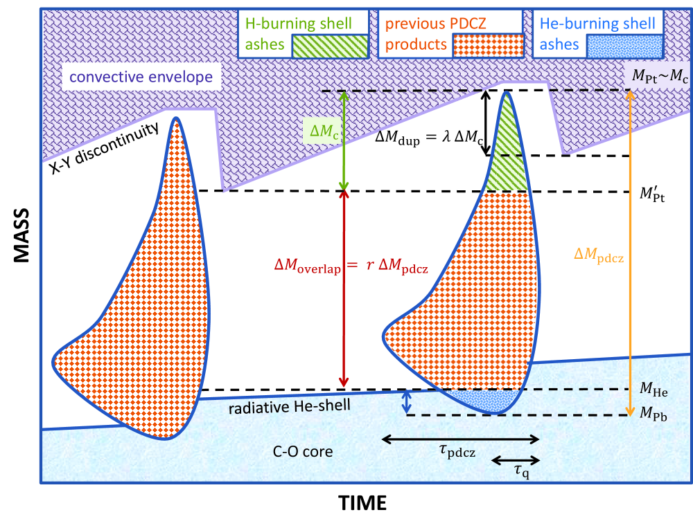
Figure 3: Sketch of the Kippenhahn diagram showing the evolution of the inner layers of a TP-AGB star during and between two consecutive thermal pulses. Mass boundaries and relevant quantities (e.g. the degree of overlap $r$ and the efficiency of the third dredge-up $\lambda$) are indicated. We refer to Table 2 for operative definitions. Note that mass and time coordinates are not on real scales, for graphical clarity. The hatched areas over the later PDCZ correspond to the three-zone stratification of the material just before the development of the convective pulse, containing from top to bottom: the ashes left by the H-burning shell, the products of the previous PDCZ, and the hashes left by the He-burning shell. On the abscissa we show the lifetime of the convective pulse $\tau_{\rm PDCZ}$, and the quenching time $\tau_{\rm q}$ counted from the maximum extension of the PDCZ.

Operatively, let us denote with $T_{\rm dup}$ the parameter representing the minimum temperature that the envelope base must exceed to activate the third dredge-up, that is:

$$T_{\rm bce}^{\rm max}\geq T_{\rm dup}\,.$$ (22)

In order to check it, at each thermal pulse, we integrate our envelope model described in Sect. 3.5.1. These numerical integrations are computed under particular conditions, namely: i) we set $\varepsilon_{\rm nuc}=\varepsilon_{\rm pp}+\varepsilon_{\rm CNO}=0$, since at this stage the H-burning shell is extinguished; ii) the two inner boundary conditions Eqs. (16) and (17) are replaced with

$$M(R_{\rm c})=M_{\rm c}\,.$$ (23)

This condition means that the mass of the degenerate core is equal to the mass contained inside the radius of a warm white dwarf, $R_{\rm c}=\delta\times R_{\rm WD}$. In the latter expression $R_{\rm WD}$ is the radius of a zero-temperature white dwarf (WD) with mass $M=M_{\rm c}$, while the coefficient $\delta>1$ accounts for the fact that the nearly isothermal degenerate core is warm, i.e. it has a non-zero temperature. To compute $R_{\rm c}$ we follow the same prescriptions as in Marigo et al. (1999), and adopt the $M_{\rm c}-L_{\rm P}$ relation of Wagenhuber & Groenewegen (1998).

Then, for given stellar mass, core mass, surface chemical composition, and peak-luminosity $L_{\rm P}$, envelope integrations are performed iterating on the effective temperature, $T_{\rm eff}$, until when $M(R_{\rm c})=M_{\rm c}$. At this point, the structure of the envelope is entirely and uniquely determined.

Since the typical values of $T_{\rm N}^{\rm min}$ may vary between different sets of models (reflecting its dependence on the adopted input physics and on the description of convection), we take $T_{\rm dup}$ as a free parameter. An advantage is that with the condition given by Eq. (22) we can also test the eventual quenching of the third dredge-up due, for instance, to a drastic reduction of the envelope mass, without the need for another external assumption (see Sect. 4.1). For the present set of TP-AGB models we have adopted the temperature parameter $\log(T_{\rm dup})=6.40$.

3.6.2 Pulse-driven nucleosynthesis

We have developed a simplified model to predict the intershell chemical composition produced by the flash-driven nucleosynthesis, using an approach similar in some aspects to those proposed by Iben & Truran (1978), Mowlavi (1999a, b), and Denissenkov & Herwig (2003).

The assumed scheme for the pulse-driven convection zone (PDCZ) is sketched with the aid of a Kippenhahn diagram in Fig. 3, showing the time evolution of the PDCZ borders from its appearance to its final quenching. Several relevant variables are defined in Table 2.

Table 2: Characteristic quantities of the TP-AGB model

$Z_{\rm i}$	initial (zero-age-main-sequence) metallicity (mass fraction)
$Y_{\rm i}$	initial (zero-age-main-sequence) helium abundance (mass fraction)
$X_{\rm i}$	initial (zero-age-main-sequence) hydrogen abundance (mass fraction)
$Z$	current metallicity (mass fraction)
$M_{\rm c}$	current core mass $\equiv$ mass of the H-exhausted core
$M_{\rm c,1}$	core mass at the first thermal pulse
$M_{\rm c,nodup}=M_{\rm c,1}+\displaystyle{\int_{0}^{t}\frac{dM_{\rm c}}{dt^{\prime}}dt^{\prime}}$	core mass in absence of the third dredge-up, where $t=0$ is the time of the first TP.
$M_{\rm i}$	initial stellar mass at the zero-age main sequence
$M_{1}$	stellar mass at the first thermal pulse
$M$	current stellar mass
$T_{\rm bce}$	temperature at the base of the convective envelope
$\tau_{\rm ip}$	interpulse period
$\phi\equiv t/\tau_{\rm ip}$ $(0\leq\phi\leq 1)$	pulse-cycle phase; the time $t=0$ refers to the quiescent pre-flash luminosity maximum.
Quiescent interpulse evolution
$\Delta M_{\rm c,tpc}$	core mass growth over one interpulse period
$\Delta M_{\rm c}=M_{\rm c}-M_{\rm c,1}$	cumulative core mass growth since the $1^{\rm st}$ TP
$\Delta M_{\rm c,nodup}=M_{\rm c,nodup}-M_{\rm c,1}$	cumulative core mass growth in absence of the third dredge-up
Pulse-driven convective zone
$M_{\rm Pt}$	mass coordinate of the top of the current PDCZ at its maximum extension
$M_{\rm Pt}^{\prime}$	mass coordinate of the top of the previous PDCZ at its maximum extension
$M_{\rm He}$	mass coordinate of the He-exhausted core
$M_{\rm Pb}$	mass coordinate of the bottom of the current PDCZ at its maximum extension
$f_{\rm ov}$	parameter to mimic overshoot applied to the bottom of the PDCZ
$\Delta M_{\rm pdcz}$	PDCZ mass at its maximum extension
$\tau_{\rm pdcz}$	total duration of the PDCZ
$\tau_{\rm q}$	quenching time since maximum extension
$T_{\rm pdcz}^{\rm max}$	maximum temperature reached in a TP at the inner border of the PDCZ
$\rho_{\rm pdcz}^{\rm max}$	maximum density reached in a TP at the inner border of the PDCZ
The third dredge-up
$M_{\rm c}^{\rm min}$	minimum core mass for the occurrence of the third dredge-up
$M_{\rm c}^{\rm 3dup}$	actual core mass at the first episode of the third dredge-up
$T_{\rm N}^{\rm min}$	minimum temperature reached by the pulse at the stage of post-flash luminosity maximum
$T_{\rm dup}$	minimum temperature at the base of the convective envelope for the occurrence of the third dredge-up
$\Delta M_{\rm dup}$	dredged-up mass at a given thermal pulse
$\Delta M_{\rm overlap}=M_{\rm Pt}^{\prime}-M_{\rm He}$	overlap mass between two consecutive PDCZs
$\lambda=\displaystyle{\frac{\Delta M_{\rm dup}}{\Delta M_{\rm c,tpc}}}$	efficiency of the third dredge-up
$r=\displaystyle{\frac{\Delta M_{\rm overlap}}{\Delta M_{\rm pdcz}}}$	degree of overlap between two consecutive PDCZ

At the onset of each TP the quantities $\Delta M_{\rm pdcz}$, $\tau_{\rm pdcz}$, $\tau_{\rm q}$, $T_{\rm pdcz}^{\rm max}$, $\rho_{\rm pdcz}^{\rm max}$ are preliminarily computed with the aid of analytic relations as a function of the core mass and metallicity, that can be obtained as fits to full AGB models (see Sect. 4 for more details). For the present work we use mainly the results by Iben & Truran (1978), Wagenhuber (1996), Karakas, Lattanzio & Pols (2002), Straniero et al. (2003).

A nuclear network is set up which includes the triple-$\alpha$ reaction and the most important $\alpha$-captures listed in Table 1. Among them we consider the main reactions which may be important as neutron sources: $\rm\,{}^{13}\kern-0.8pt{C}\,({{}^{4}He}\,,{n})\,{}^{16}\kern-0.8pt{O}\,$, $\rm\,{}^{17}\kern-0.8pt{O}\,({{}^{4}He}\,,{n})\,{}^{20}\kern-0.8pt{Ne}\,$, $\rm\,{}^{18}\kern-0.8pt{O}\,({{}^{4}He}\,,{n})\,{}^{21}\kern-0.8pt{Ne}\,$, $\rm\,{}^{21}\kern-0.8pt{Ne}\,({{}^{4}He}\,,{n})\,{}^{24}\kern-0.8pt{Mg}\,$, $\rm\,{}^{22}\kern-0.8pt{Ne}\,({{}^{4}He}\,,{n})\,{}^{25}\kern-0.8pt{Mg}\,$, and $\rm\,{}^{25}\kern-0.8pt{Mg}\,({{}^{4}He}\,,{n})\,{}^{28}\kern-0.8pt{Si}\,$.

At time $t=0$, just before the development of a TP, the chemical composition of the region over which the flash-driven convection will extend, is assumed to be stratified over three zones:

1. $M_{\rm Pt}-M_{\rm Pt}^{\prime}$ containing the ashes, with abundances $\{X_{\rm Hb}\}$, left by the quiescent radiative H-shell over the previous interpulse period;

2. $M_{\rm Pt}^{\prime}-M_{\rm He}$ containing the nuclear products of the PDCZ developed during the previous TP;

3. $M_{\rm He}-M_{\rm Pb}$ containing the products of radiative He burning.

For simplicity each of the three zones is assigned an average chemical composition, though a chemical profile exists in the a) and c) regions where nuclear burning has occurred in radiative conditions.

Denoting with $X^{\rm s}$ the homogeneous surface abundances, the composition of the hydrogen free layer left by the H-burning shell is estimated following the indications by Mowlavi (1999a, b), which can be summarised as follows:

• all hydrogen is burnt into helium: $X_{\rm Hb}({\rm H})=0$;

• all available CNO isotopes are converted into ¹⁴N: $X_{\rm Hb}(^{14}{\rm N})=14\times\sum_{i=12}^{i=18}X_{i}^{\rm s}/A_{i}$ (where $A_{i}$ is the mass number);

• all ²²Ne is burnt into ²³Na by the NeNa chain: $X_{\rm Hb}(^{22}{\rm Ne})=0$;

• the abundance of ${}^{23}{\rm Na}$ is computed with:
  $X_{\rm Hb}(^{23}{\rm Na})=f_{\rm Na}[23/22\times X^{\rm s}(^{22}{\rm Ne})+X^{\rm s}(^{23}{\rm Na})]$.

The factor $f_{\rm Na}$ accounts for the possible destruction of ²³Na by proton captures at $T>6\times 10^{7}$ K. Its value typically ranges from $f_{\rm Na}=1$ (no destruction) down to $f_{\rm Na}=0.2$ (see figure A.3 in Mowlavi, 1999a). For the present set of calculations we have adopted $f_{\rm Na}=1$. The effects of the Mg-Al chain on the resulting $X_{\rm Hb}$ abundances is not considered in this work, and it will be implemented in a future study.

During each TP we follow the progressive development of pulse convection and related nucleosynthesis, over the duration $\tau_{\rm pdcz}$. The process is divided into two consecutive phases:

1. from the onset of the PDCZ at time $t=0$ up to maximum extension at time $t=\tau_{\rm pdcz}-\tau_{\rm q}$;

2. from maximum PDCZ extension to final pulse quenching at time $t=\tau_{\rm pdcz}$, with duration $\tau_{\rm q}$.

The PDCZ is resolved both in time and in space. The entire duration $\tau_{\rm pdcz}$ is subdivided in typically $\simeq 100$ time steps, while at each time a suitable grid of mass meshes is set up across the current PDCZ, with a maximum mass resolution of $\simeq 10^{-4}\,M_{\odot}$. The evolution of $T_{\rm pdcz}^{\rm max}$ and $T_{\rm rho}^{\rm max}$ over $\tau_{\rm pdcz}$, and the temperature and density stratifications across the PDCZ mass are described on the basis of detailed calculations of thermal pulses (Wagenhuber, 1996; Wagenhuber & Groenewegen, 1998, and private communications). Illustrative examples are discussed later, in Sect. 7.5.

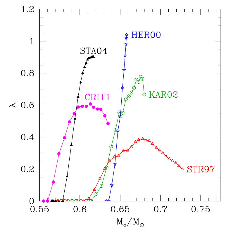
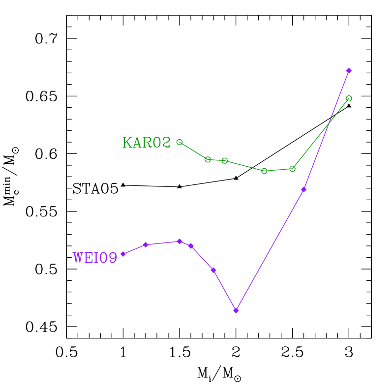
Figure 4: Left panel: Efficiency $\lambda$ of the third dredge-up as a function of the current core mass during the TP-AGB evolution of a stellar model with initial mass $M_{\rm i}=3.0\,M_{\odot}$ and metallicity $Z_{\rm i}=0.02$. Right panel: Minimum core mass $M_{\rm c}^{min}$ for the third dredge-up as a function of the stellar mass for TP-AGB models with initial metallicity $Z_{\rm i}=0.008$. Predictions from full AGB calculations of various authors are compared, namely: CRI11 (Cristallo et al., 2011); WEI09 (Weiss & Ferguson, 2009); STA05 (Stancliffe, Izzard & Tout, 2005); STA04 (Stancliffe, Tout & Pols, 2004); KAR02 (Karakas, Lattanzio & Pols, 2002); HER00 (Herwig, 2000); STR97 (Straniero et al., 1997). Note the large differences from author to author both in $\lambda$ and in $M_{\rm c}^{\rm min}$.

During the phase I the evolution of the PDCZ is followed by cycling over the sequence of steps: nucleosynthesis $\rightarrow$ homogenization $\rightarrow$ expansion/recession$\rightarrow$ homogenization. At each time step, starting from the current PDCZ bottom (with mass coordinate $m_{\rm Pb}$) up to the current PDCZ top border (with mass coordinate $m_{\rm Pt}$) the nuclear network is solved locally in each mesh point.

A homogeneous chemical composition is assigned to the PDCZ by mass-averaging the mesh abundances. Then, the PDCZ is made expand i.e. inner/upper borders of the PDCZ are shifted inward/outward, and elements of new material, stratified according to the initial composition, are engulfed. Eventually, a new PDCZ composition is obtained by averaging the abundances with weights proportional to the masses of the corresponding meshes.

The entire process, i.e. convective burning followed by expansion and homogenization, is iterated until the maximum extension is reached, i.e. $m_{\rm Pb}=M_{\rm Pb}$ and $m_{\rm Pt}=M_{\rm Pt}$, and the mass contained in the PDCZ is equal to $\Delta M_{\rm pdcz}$. At this point $t=\tau_{\rm pdcz}-\tau_{\rm q}$.

The quenching phase II is described by a similar scheme, except that now the PDCZ convection retreats and the inner/upper borders are shifted outward/inward until $t=\tau_{\rm pdcz}$. The nuclear network is integrated over the pulse quenching phase and a final homogeneous chemical composition is obtained. This sets the chemical mixture of the material that may be brought up to the surface by the subsequent third dredge-up phase.

Despite its simplicity the PDCZ model yields results that nicely agree with those of full TP-AGB computations. A detailed discussion of the predictions and their main dependencies is given in Sect. 7.5.

4 The synthetic module

Most analytical ingredients of the COLIBRI code are formulas accurately fitting the results of full AGB models covering wide ranges of initial stellar mass and metallicity. The formulas are taken either from the extensive compilations by Wagenhuber (1996); Wagenhuber & Groenewegen (1998); Karakas, Lattanzio & Pols (2002); Izzard et al. (2004, 2006), and other sources (Straniero et al., 2003), or they are directly derived from AGB model data sets by using standard $\chi^{2}$-minimization techniques. New fits can be found in Appendix A.

Importantly, all these analytic relations include a metallicity dependence, and take into account the peculiar behaviour of the first sub-luminous pulses while approaching the full-amplitude regime.

Among the most important prescriptions we mention the flash-driven luminosity variations as a function of the pulse-cycle phase (Wagenhuber & Groenewegen, 1998), the core mass-interpulse period relation (Wagenhuber & Groenewegen, 1998), the maximum mass of the PDCZ and its duration, the maximum temperature attained at the bottom of the PDCZ during a TP (Karakas & Lattanzio, 2007), the efficiency $\lambda$ of the third dredge-up (Karakas, Lattanzio & Pols, 2002).

Due to their particular relevance, below we will discuss in more detail a few analytic relations adopted in the present version of COLIBRI.

4.1 The third dredge-up: the need for a parametric description

It is common practice describing the third dredge-up by means of two characteristic quantities, namely:

• $M_{\rm c}^{\rm min}$: the minimum core mass for the onset of the third dredge-up;

• $\lambda=\displaystyle\frac{\Delta M_{\rm dup}}{\Delta M_{{\rm c,tpc}}}$: the efficiency of the third dredge-up, defined as the fraction of the core-mass growth over the interpulse period that is dredged-up to the surface at the next TP.

Compared to earlier computations, recent full TP-AGB evolutionary models have allowed a wide exploration of the third dredge-up characteristics as a function of stellar mass and metallicity (e.g. Karakas, Lattanzio & Pols, 2002; Herwig, 2000, 2004a, 2004b; Weiss & Ferguson, 2009; Cristallo et al., 2011). A few general trends can be extracted from these calculations.

The efficiency $\lambda$ is expected to increase with stellar mass $M$, such that TP-AGB stars with initial masses $M>3\,M_{\odot}$ are predicted to reach $\lambda\simeq 1$, which implies no, or very little, core mass growth. Lower metallicities favour an earlier onset of the third dredge-up and a larger efficiency, resulting in an easier formation of low-mass carbon stars. Full TP-AGB models exist which are found to reproduce, or at least to be reasonably consistent with, basic observables, such as the luminosity functions of carbon stars in the Magellanic Clouds (e.g. Stancliffe, Izzard & Tout, 2005; Weiss & Ferguson, 2009; Cristallo et al., 2011).

Together with these improvements, present TP-AGB models also document that the third dredge-up is plagued by severe theoretical uncertainties. They are due mainly to our still deficient knowledge of convection and mixing, as well to a nasty sensitivity of the depth of the third dredge-up to technical and numerical details (see Frost & Lattanzio 1996, and Mowlavi 1999b for thorough analyses).

As a consequence we still lack a robust assessment for $M_{\rm c}^{\rm min}$ and $\lambda$, and these parameters are found to vary considerably from author to author even for the same combination ($M_{\rm i}$, $Z_{\rm i}$) of initial stellar mass and metallicity. The theoretical dispersion is exemplified in Fig. 4. The dynamical ranges of the parameters covered by the various sets of computations are large, amounting to almost a factor of 3 for the maximum $\lambda$ attained in a ($M_{\rm i}=3.0\,M_{\odot}$, $Z_{\rm i}=0.02$) model, and more than $\simeq 0.1\,M_{\odot}$ for $M_{\rm c}^{\rm min}$ for the ($M_{\rm i}=2.0\,M_{\odot}$, $Z_{\rm i}=0.008$) case. It is clear that these variations propagate dramatically in terms of the predicted stellar properties: significant differences are expected in the luminosities spanned during the C star phase, the final masses, the chemical yields, etc. The situation appears even more unclear considering, for instance, that two independent sets of calculations, i.e. Stancliffe, Izzard & Tout (2005) and Weiss & Ferguson (2009), with largely different predictions for $M_{\rm c}^{\rm min}$ (see the right-hand side panel of Fig. 4) are found by the authors to recover the same observable, i.e. the carbon star luminosity function in the LMC. This uncomfortable convergence of the results is likely due to the combination of other critical parameters (e.g. efficiency $\lambda$, and mass loss). In fact, it is differences in details of the chosen input physics, such as the treatment of convective boundaries and the inclusion or not of overshoot, that produces most of the variations seen in full models, such as those shown in Fig. 4.

All these reasons amply justify the approach of taking $\lambda$ and $M_{\rm c}^{\rm min}$ (or, in alternative, $\lambda$ and the temperature parameter $T_{\rm dup}$; see Sect. 3.6.1), as free parameters, and to calibrate them with the largest possible set of observations to reduce the likely degeneracy between different factors.

4.2 Properties of the pulse-driven convection zone

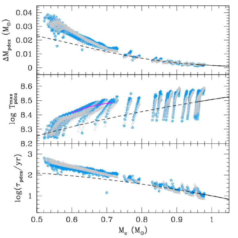
Figure 5: Characteristic quantities of the pulse-driven convection zone, i.e. maximum mass, maximum bottom temperature, and duration, as a function of the core mass. A large set of $1658$ models from Karakas & Lattanzio (2007), corresponding to various choices of stellar mass and metallicity, is plotted (blue stars), together with our synthetic predictions (grey triangles) for the same stellar parameters. Other fitting relations are shown for comparison. The Straniero et al. (2003) relation (magenta solid line) for $T_{\rm pdcz}^{\rm max}$ corresponds to a model with $M_{\rm i}=2.0\,M_{\odot},\,Z_{\rm i}=0.02$ and the core mass increasing from $0.60\,M_{\odot}$ to $0.72\,M_{\odot}$. The Iben & Truran (1978) relations (black line) are strictly valid for high core masses $(0.96\la M_{\rm c}/M_{\odot}\la 1.33)$ (solid line portion), but they have been extrapolated to lower $M_{\rm c}$ (dashed line portion) for illustrative purpose only.

In Fig. 5 we show three key quantities of the PDCZ as a function of the core mass (starred symbols), as predicted by Karakas, Lattanzio & Pols (2002); Karakas & Lattanzio (2007) for five values of the initial metallicity $(Z_{\rm i}=0.0001,\,Z_{\rm i}=0.004,\,Z_{\rm i}=0.008,\,Z_{\rm i}=0.012,\,{\rm and}\,Z_{\rm i}=0.02)$. Superimposed we plot the results obtained with the analytic relations (grey triangles) for the same stellar parameters ($M_{\rm i}$, $M_{\rm c}$, and $Z_{\rm i}$) as in the original full computations, The fitting relations behave well all over the core-mass range covered by the full models. The formulas and their coefficients are given in Appendix A.

For comparison we draw two more relations taken from literature, namely Iben & Truran (1978, black line) and Straniero et al. (2003, magenta solid line). We have extrapolated the Iben & Truran (1978) relations over the whole $M_{\rm c}$ range, but one should consider that they were originally derived from the high core mass $(0.96\la M_{\rm c}/M_{\odot}\la 1.33)$ AGB models of Iben (1977). We see that for $M_{\rm c}\ga 0.85\,M_{\odot}$ the Iben & Truran (1978) relations for $\Delta M_{\rm pdcz}$ and $\tau_{\rm pdcz}$ are in general agreement with the average trend predicted by the recent AGB computations of Karakas & Lattanzio (2007). The earlier results of Iben (1977) for $T_{\rm pdcz}^{\rm max}$ are systematically lower by up to $0.6-0.8$ dex.

The other relation proposed by Straniero et al. (2003), on the basis of their full AGB calculations, appears to be consistent with the Karakas & Lattanzio (2007) results inside its validity range, (i.e. $0.6\la M_{\rm c}/M_{\odot}\la 0.7$). However, we notice that it does not allow to describe the initial rise of the temperature typical of the first pulses.

5 Tests: COLIBRI vs full stellar models

5.1 Effective temperature and convective-base temperature

As a first test we compare the effective temperatures obtained with COLIBRI from envelope integrations (the method is outlined in Sect. 3.5.1), against the predictions of full stellar models computed with PARSEC (Bressan et al., 2012). A detailed discussion is given in Appendix B.

Figure 6 quantifies the comparison in relation to the quiescent stage just preceding the occurrence of the $1^{\rm st}$ thermal pulse for several values of stellar masses and metallicities. We see that the differences are in most cases quite low, amounting to few tens of degrees, well below the typical observational errors for $T_{\rm eff}$ of AGB stars, about equal to $\pm(100-200)$ K.

The results shown in the two panels of Fig. 6 differ in the chemical distributions of metals assumed in COLIBRI. They are usually expressed in terms of the ratios $X_{i}/Z$, where $X_{i}$ denotes the fractional mass of a given metal $i$. While in one case (top panel) both EoS and opacities are computed with the ÆSOPUS and Opacity Project codes adopting, for each model, the actual set of surface abundances predicted by PARSEC at the $1^{\rm st}$ TP, in the other case (bottom panel) the mixtures are assumed to be all scaled-solar for any metallicity, i.e. $X_{i}/Z=X_{i,\odot}/Z_{\odot}$ for each metal $i$.

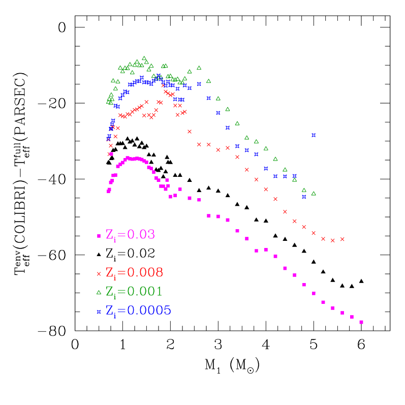
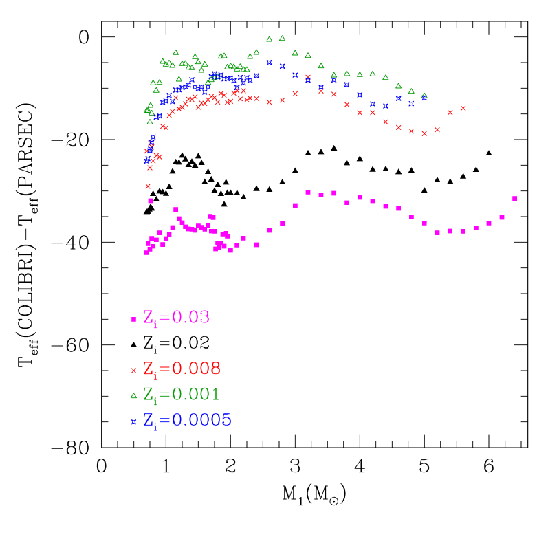
Figure 6: Differences in the predicted effective temperature between the envelope-integration method adopted in the COLIBRI code and the PARSEC full evolutionary calculations. All models refer to the pre-flash luminosity maximum just before the $1^{\rm st}$ TP for several choices of the initial stellar mass and metallicity. Top panel: The COLIBRI results are obtained with on-the-fly ÆSOPUS and Opacity Project computations for the EoS and opacities, consistently coupled to the actual chemical abundances across the “deep” envelope. Bottom panel: The COLIBRI predictions are derived adopting a distributions of metals frozen to the scaled-solar ratios for all metallicities, i.e. $X_{i}/Z=X_{i,\odot}/Z_{\odot}$, as assumed in PARSEC.

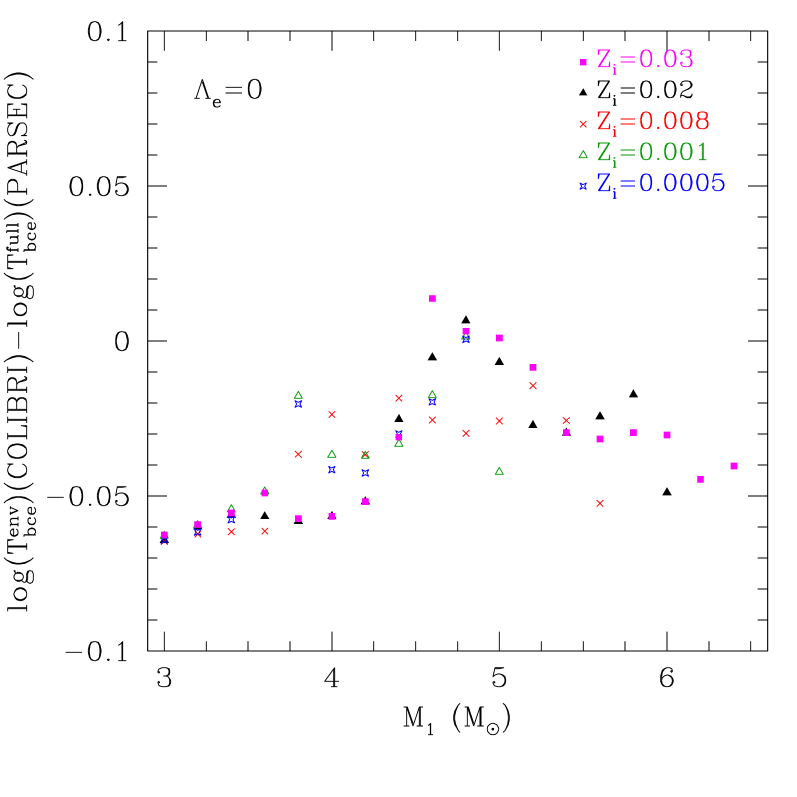
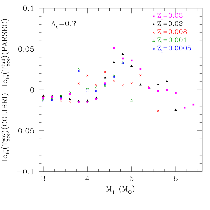
Figure 7: Differences in the predicted temperature at the base of the convective envelope between the envelope-integration method adopted in the COLIBRI code and the PARSEC full evolutionary calculations. All models refer to the pre-flash luminosity maximum just before the $1^{\rm st}$ TP for several choices of the initial stellar mass and metallicity. Top panel: COLIBRI models are computed adopting the classical Schwarzschild criterion to define the inner border of the convective envelope. Bottom panel: The COLIBRI predictions are derived with convective overshoot at the base of the envelope, extending over a distance $l_{\rm ov}=\Lambda_{\rm e}\times H_{P}$ (where $H_{P}$ is the pressure-scale height), with $\Lambda_{\rm e}=0.7$ as assumed in PARSEC.

In principle, the former case is the correct one as it couples consistently EoS and opacities with the current metal abundances, that may have varied with respect to the values at the zero-age main sequence, following the $1^{\rm st}$ and second dredge-up processes. On the other hand, the latter case, which is also adopted in the PARSEC models and, more generally, by most full stellar codes, neglects the variation of the elemental ratios, e.g. the lowering of the C/O, due to mixing episodes prior to the TP-AGB phase.

It follows the accuracy degree of COLIBRI against PARSEC is best represented by the temperature differences in the bottom panel of Fig. 6, since the same metal ratios, $X_{i}/Z=X_{i,\odot}/Z_{\odot}$, are assumed in both sets of computations. In fact, passing from the top to the bottom panel of Fig. 6 it is evident that the agreement between the COLIBRI and PARSEC predictions improves, particularly for models of larger masses which are most affected by the second dredge-up. A more detailed discussion of this aspect and other related effects can be found in Appendix B.1.

The temperature at the base of the convective envelope, $T_{\rm bce}$, provides an additional test for our envelope-integration method, and it is particularly relevant for massive AGB models ($M>4\,M_{\odot}$) as it measures the efficiency of HBB. As analysed in Appendix B.2, the results are affected by several technical details not dealing with the envelope integration method, such as differences in the operative definition of the convective border, inclusion or not of convective overshooting, assumed metal partitions, adopted equation of state, high-temperature opacities, etc. All these aspects, together with the fact that the base of the convective envelope may fall inside a region characterized by an extremely steep temperature gradient, concur to somewhat amplify the differences in $T_{\rm bce}$.

Figure 8 shows the temperature differences between COLIBRI and PARSEC predictions for initial masses $M_{\rm i}\geq 2.6\,M_{\odot}$ and various metallicities. Two cases are considered in the COLIBRI definition of the innermost stable mesh-point of the convective envelope, namely: the strict application of the Schwarzschild criterion (top panel), and the inclusion of convective overshoot by the same amount as adopted in PARSEC (bottom panel). In both cases the differences remain fairly small, i.e. $|\log(T_{\rm bce}^{\rm full})-\log(T_{\rm eff}^{\rm env})|<0.05$ dex.

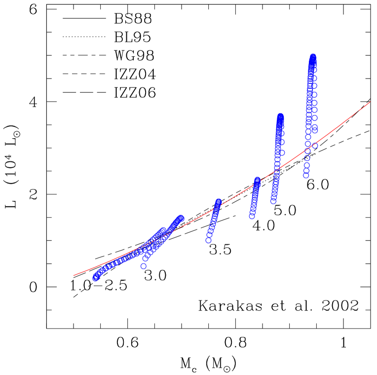
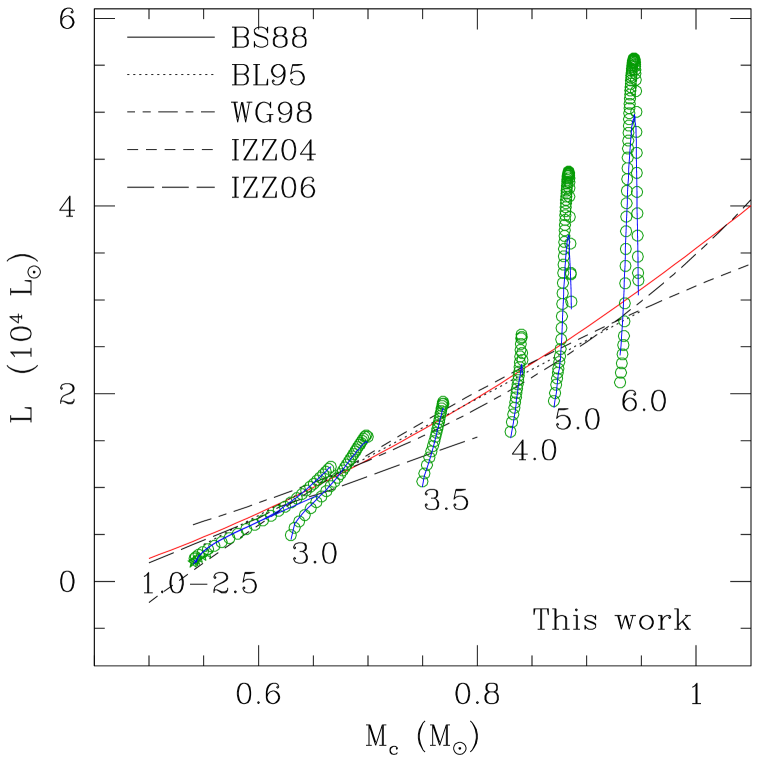
Figure 8: Stellar luminosity as a function of the core mass at the quiescent pre-flash stage preceding each thermal pulse, for two sets of TP-AGB models with initial metallicity $Z_{\rm i}=0.008$. Left-hand side panel: full TP-AGB models by Karakas, Lattanzio & Pols (2002) (empty blue circles). Right-hand side panel: predictions of our deep envelope integrations that include the H-burning shell (empty green circles). To facilitate comparison we overplot the Karakas, Lattanzio & Pols (2002) predictions (solid blue lines). The initial stellar masses (in $M_{\odot}$) are quoted nearby the corresponding sequences. A few CMLRs from various authors are also plotted, namely: Boothroyd & Sackmann (1988a, BS88), Blöcker (1995, BL95), Wagenhuber & Groenewegen (1998, WG98), Izzard et al. (2004, IZZ04), Izzard et al. (2006, IZZ06). Note the effect of HBB which makes more massive TP-AGB models to deviate significantly from the CMLRs towards higher luminosities. See text for more details.

In conclusion our tests indicate that:

• the agreement in effective temperatures between our envelope integrations and full stellar modelling is extremely good, with differences $|T_{\rm eff}^{\rm env}-T_{\rm eff}^{\rm full}|<40$ K and in many cases practically negligible;

• the differences $T_{\rm eff}^{\rm env}-T_{\rm eff}^{\rm full}$ are always negative and tend to systematically decrease at lower metallicity, suggesting that they are likely related to the elemental abundances and the way they are treated in the EoS and opacity computations. Indeed cooler $T_{\rm eff}^{\rm env}$ compared to $T_{\rm eff}^{\rm full}$ are partly explained by the differences in the assumed $X_{i}/Z$ used in the EoS and opacities, i.e. actual chemical abundances in COLIBRI against frozen scaled-solar ratios adopted by PARSEC.

• A very good agreement is found also for $T_{\rm bce}$ (within $0.05$ dex), which strongly supports the ability of our envelope-integration method to account correctly for the occurrence of HBB in more massive AGB models.

5.2 Quiescent luminosity on the TP-AGB

Thanks to the extension of the deep envelope model to include the H-burning shell, we can predict the luminosity during the quiescent stages without adopting any auxiliary CMLR, as usually done in synthetic TP-AGB models (e.g. Hurley, Pols & Tout, 2000; Izzard et al., 2004, 2006; Cordier et al., 2007; Marigo & Girardi, 2007).

Figure  8 shows the pre-flash luminosity as a function of the core mass for two sets of TP-AGB models with initial metallicity $Z_{\rm i}=0.008$ and a few values of the initial stellar mass, computed by Karakas, Lattanzio & Pols (2002), and with the COLIBRI envelope-integration technique adopting the same stellar parameters (e.g. total mass, core mass, dredged-up mass, mixing-length parameter, and initial metallicity). Considering that the two sets of calculations differ both in technical details (e.g. solution method of the stellar structure equations, zone-meshing, etc.) and in the input physics (e.g. EoS, opacities, nuclear reaction rates, etc.) the overall agreement is quite striking. We derive two main implications: i) in absence of HBB, i.e. for TP-AGB models with smaller cores ($M_{\rm c}\la 0.75\,M_{\odot}$) and less massive envelopes ($M_{\rm env}\la 2.5\,M_{\odot}$), the CMLR is a robust prediction of the theory (essentially reflecting the thermostatic character of the H-burning shell), ii) in our deep envelope integrations the treatment of the H-burning energetics is reliable.

In fact, in the range $0.5\,M_{\odot}\la M_{\rm c}\la 0.7\,M_{\odot}$ our predictions for the pre-flash luminosity maximum recover the Karakas, Lattanzio & Pols (2002) results remarkably well, and more generally the classical CMLRs (e.g. Boothroyd & Sackmann, 1988a, red line). The brightening of the tracks beyond the CMLR, as shown by Karakas, Lattanzio & Pols (2002) models with $M_{\rm c}\la 0.75\,M_{\odot}$ and $M\la 3.5\,M_{\odot}$, is driven by the occurrence of a deep third dredge-up. This effect is discussed in Sect. 5.2.1.

At larger core masses, $M_{\rm c}\ga 0.75\,M_{\odot}$ (see the models with initial masses $M_{\rm i}=4,\,5,\,6\,M_{\odot}$ in Fig. 8), HBB is expected to produce the break-down of the CMLR: similarly to the tracks by Karakas, Lattanzio & Pols (2002), the COLIBRI sequences with $M\geq 4\,M_{\odot}$ exhibit a steep luminosity increase at almost constant core mass ($\lambda\simeq 1$ in these models). After reaching a maximum, the luminosity starts to decline quickly from pulse to pulse until the CMLR is recovered again. The luminosity peak and the subsequent decrease are controlled by the onset of the super-wind phase, which determines a rapid reduction of the envelope mass, hence the weakening and eventual extinction of HBB. We note that the COLIBRI tracks with HBB reach higher luminosity maxima than the Karakas, Lattanzio & Pols (2002) models with the same initial masses, a circumstance that confirms the sensitivity of the HBB process on the adopted input physics and details of the convection treatment (Ventura & D’Antona, 2005).

5.2.1 The effect of deep third dredge-up

Full AGB calculation indicate that the occurrence of deep dredge-up events make the models brighter than expected by the CMLR (Herwig, Schoenberner & Bloecker, 1998; Mowlavi, 1999b; Karakas, Lattanzio & Pols, 2002), due to the intervening non-linear relation between the core mass and the core radius.

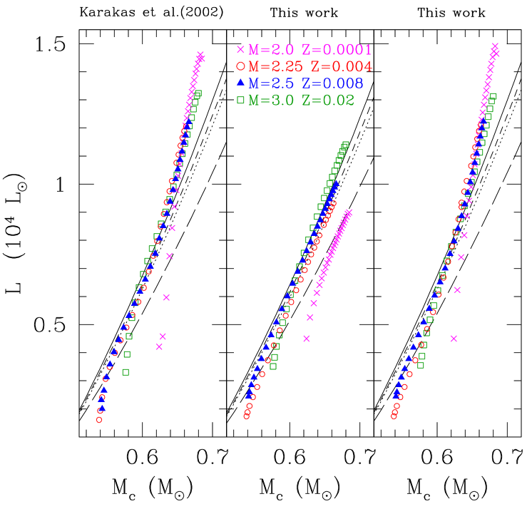
Figure 9: Quiescent pre-flash luminosity maximum as a function of the core mass for a few combinations of initial masses (in $M_{\odot}$) and metallicities $Z_{\rm i}$, as indicated in the middle panel. Left panel: Results from full TP-AGB models taken from Karakas, Lattanzio & Pols (2002); Karakas & Lattanzio (2007) Note the steep increase of the luminosities beyond the CMLRs, which is interpreted as an effect driven by the third dredge-up. Middle panel: Results from deep envelope integrations described in Sect. 3.5.1. The boundary condition Eq. (17) is used with the temperature corresponding to the true core mass, $M_{\rm c}$. Right panel: Results from deep envelope integrations described in Sect. 3.5.1, but with the boundary condition Eq. (17) evaluated using a fictitious core mass given by Eq. (24). For comparison, the analytic CMLR of Boothroyd & Sackmann (1988a) is plotted for metallicities $Z_{\rm i}=0.02$ (solid line), $Z_{\rm i}=0.008$ (short-dashed line), $Z_{\rm i}=0.004$ (dotted line), and $Z_{\rm i}=0.0005$ (long-dashed line).

To account for this effect we have analysed a large number of full TP-AGB models from Karakas, Lattanzio & Pols (2002). These models are characterised by a large range of dredge-up efficiencies, from $\lambda\approx 0$ to $\lambda\approx 1$, depending on stellar mass and metallicity.

We find that, in presence of dredge-up, the quiescent pre-flash luminosity $L_{\rm Q}$ of a TP-AGB model with a core mass $M_{\rm c}$ is well recovered with our envelope-integration method by applying the boundary condition for the core temperature (Eq. 17) in the form $T_{\rm c}=T(M_{\rm c}^{\rm fict})$, where we introduce a fictitious core mass

$$M_{\rm c}^{\rm fict}=M_{\rm c}+\xi\,(M_{\rm c,nodup}-M_{\rm c,1})\,,$$ (24)

with the multiplicative factor $\xi\simeq 0.3-0.4$.

The variable $M_{\rm c,nodup}$ has been already used in past synthetic TP-AGB models (e.g. Hurley, Pols & Tout, 2000; Izzard et al., 2004, 2006). It was introduced to account for effects due to an increase in core degeneracy during the quiescent interpulse growth, so that stars with the same core mass, but different dredge-up histories, may have different quiescent luminosities. Since in COLIBRI the integrations of stellar structure are performed down to the bottom of the H-burning shell, for the electron-degenerate core beneath it we need to resort to a parametrized description. The variable $M_{\rm c,nodup}$ is a suitable choice for the case under consideration.

The results are illustrated in Fig. 9, where the COLIBRI tracks computed with Eq. (24) setting $\xi=0.3$ (right-hand side panel) are compared to the original sequences Karakas, Lattanzio & Pols (2002) (left-hand side panel). Despite the simple formulation of the corrective term in Eq. (24), the agreement is quite satisfactory.

It is also instructive to look at the middle panel of Fig. 9 showing the COLIBRI predictions for $\xi=0$, i.e. without the effect of the third dredge-up. In this case all the tracks comply with the classical CMLR by Boothroyd & Sackmann (1988a), and reproduce quite well the dimming of the quiescent luminosity at decreasing metallicity. As a matter of fact, the TP-AGB models from which Boothroyd & Sackmann (1988a) derived their analytic CMLR were characterised by rather shallow, in most cases absent, convective dredge-up events, and were mostly limited to the first few thermal pulses. This fact explains why the over-luminosity effect due to the third dredge-up does not show up in the Boothroyd & Sackmann (1988a) models.

It follows that the very nice accordance between the CMLR of Boothroyd & Sackmann (1988a) and the COLIBRI predictions for $\xi=0$ adds a further confirmation on the validity of our envelope-integration method in terms of the H-burning energetics (see also Sect. 5.2).

5.3 Computational agility

A key feature of the COLIBRI code is the computational agility, that is kept to competitive levels despite the several numerical operations performed at each time step, i.e. iterative solution of the atmosphere and envelope structures, integration of nuclear networks, on-the-fly computation of the EoS and Rosseland mean opacities across all meshes.

Figure 10 compares the performance of the COLIBRI and the PARSEC codes, in terms of the typical CPU time required to compute one thermal pulse cycle, i.e. the time interval between two consecutive pre-flash luminosity maxima. The two histograms correspond to the distributions of $N^{\rm tot}_{\rm tpc}=507$ thermal pulse cycles followed over a wide range of initial stellar masses $(0.6M_{\odot}\,\la M_{\rm i}\la 6M_{\odot})$, and metallicities $(0.0005\leq Z_{\rm i}\leq 0.07)$.

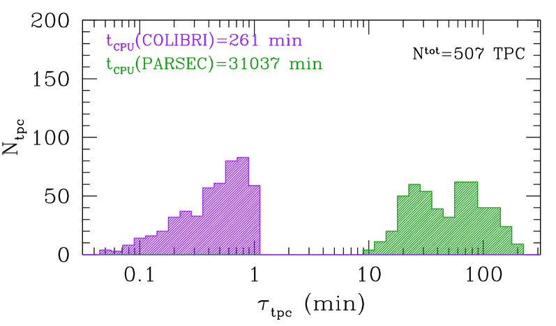
Figure 10: Distributions of CPU times relative to one thermal pulse cycle, either with the COLIBRI code (purple histogram), or with the PARSEC stellar evolution code (green histogram). In both cases the sample consists of $N=507$ complete pulse cycles.

The difference in CPU time requirements is noticeable. The COLIBRI distribution shows a broad peak at $\tau_{\rm tpc}\sim 30-40$ s, and a low tail extending down to $3-4$ s. The median of the distribution is $\tilde{\tau}_{\rm tpc}\simeq 14$ s. Bins at longer $\tau_{\rm tpc}$ are populated by TP cycles referring to i) the last TP-AGB stages in which the high mass-loss rates impose the reduction of the evolutionary time steps, and ii) more massive AGB stars experiencing both the third dredge-up and HBB, with consequent intensive computing of EoS and opacities to follow the continuous changes in the envelope chemical abundances.

The PARSEC distribution is located over much longer time scales, with $\tau_{\rm tpc}$ ranging from $\approx 10$ min to $\approx 200$ min. The median of the PARSEC distribution is $\tilde{\tau}_{\rm tpc}\simeq 29$ min.

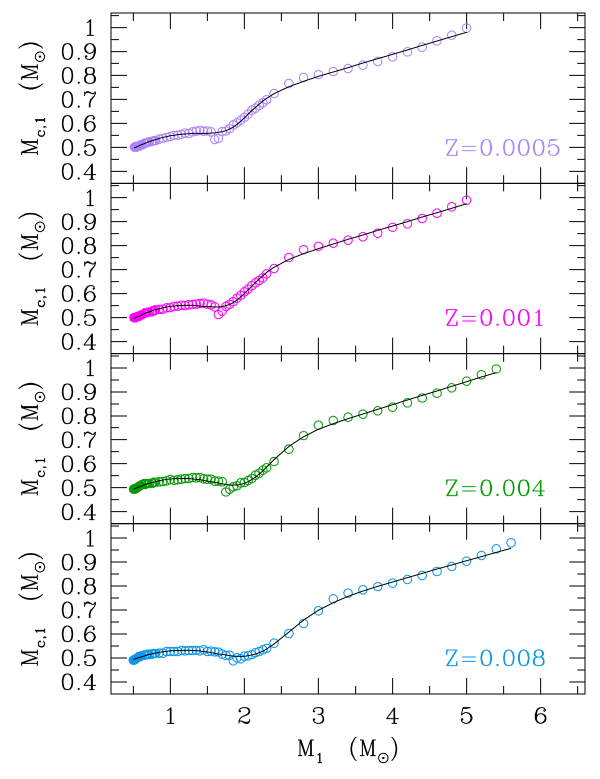
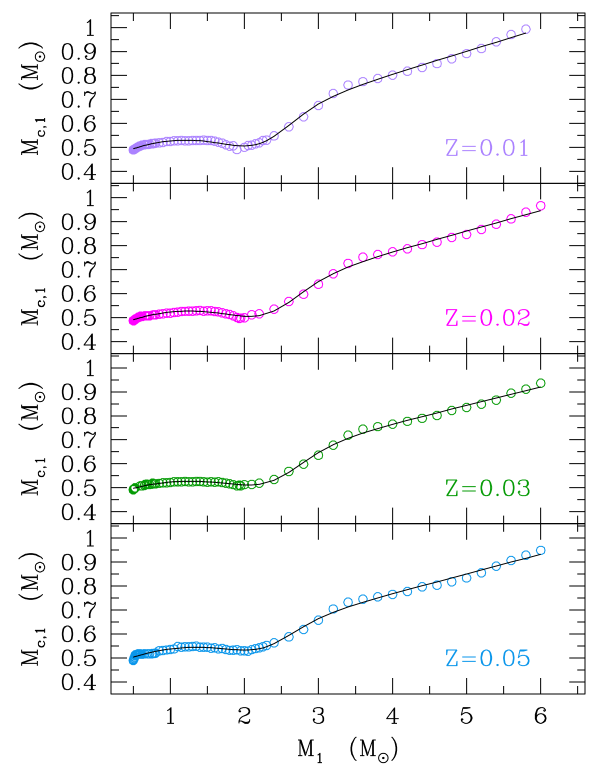
Figure 11: Core mass as a function of the stellar mass at the stage of the pre-flash luminosity maximum, just preceding the occurrence of the $1^{\rm st}$ thermal pulse. The data, extracted from the PARSEC database of stellar models (Bressan et al., 2012), are shown for eight choices of the initial metallicities, as indicated. In each panel the solid line is the fit obtained with Eq. (A.2), and the coefficients given in Table 4.

In any case, the gain in terms of CPU time with COLIBRI is sizable: the integrated CPU time to compute $N^{\rm tot}_{\rm tpc}=507$ thermal pulse cycles is roughly $4$ hours for COLIBRI and $\simeq 21$ days for PARSEC.

While we acknowledge that the continuing increase in computing speed of modern computers enables present-day full evolution codes to compute extended grids of TP-AGB tracks, we should also realize that performing a multi-parametric fine calibration of the uncertain processes/assumptions is extremely more demanding in terms of computational agility and numerical stability, characteristics that do not ordinarily apply to the full approach.

Processes and assumptions that are known to dramatically affect the TP-AGB evolutionary phase are, for instance, mass loss, third dredge-up, nucleosynthesis, convection efficiency, overshooting, initial chemical abundances, etc. For each of them, we could single out more than one characteristic parameter, depending on the theoretical picture one aims investigating at. A dozen parameters may represent a reasonable estimate of the number of factors one should take into consideration for an extensive analysis.

To get an order of magnitude of the time requirements, let us consider our specific working case. At present we are dealing with $14$ metallicity sets (limited to the scaled-solar compositions, other sets are planned), from very low to super-solar $Z$. From the PARSEC database of models, we extract the initial conditions at the first TP for $65-70$ values of the initial stellar mass (on average), from $\simeq 0.5\,M_{\odot}$ to $\simeq 5-6\,M_{\odot}$. The fine grid in mass is important to allow for the construction of accurate and detailed stellar isochrones.

The total number of TP-AGB tracks to be calculated is $951$. With the set of parameters adopted in this exploratory work, all the TP-AGB tracks followed by COLIBRI cover $14293$ thermal pulse cycles, for a true CPU time of $7854\,{\rm s}\simeq 5.2$ days.

With the conservative assumption that the PARSEC code takes a computing time $\approx 100$ longer (probably more), the whole TP-AGB tracks would be ready after $\simeq 520$ days, that is $\approx 1.5$ yr. These are likely optimistic estimates, considering that the current PARSEC distribution of CPU times is biased towards shorter values since, in general, each evolutionary track includes the first few TPs, that usually involve a lighter computational effort compared to the later, well-developed TPs. Moreover, the PARSEC tracks are calculated at constant mass, while the inclusion of a mass-loss prescription would certainly impose a further reduction of the time steps, hence an increase of the CPU time.

It is also worth noting that the computing time request is expected to increase with the stellar mass, given that the pace at which TPs take place correlates with the core mass, while HBB gets stronger. In a recent study Siess (2010) reported that $\approx 6$ months of CPU time were required by his full evolution code to follow the whole Super-AGB phase of just one model with strong HBB. Of course, this may not be the same for other full codes, but a trend of increasing computational cost with the stellar mass is of general validity.

In any case, we emphasize here that what makes the computational effort particularly challenging for full models is the calibration process. In fact, promptly producing extended and dense (in mass and metallicity) sets of TP-AGB tracks is a necessary requisite to build accurate stellar isochrones spanning the whole relevant ranges of ages and metallicities. In turn, the stellar isochrones are the building blocks of population synthesis simulations of galaxies including AGB stars, which can be readily put in direct comparison with observations. Possible discrepancies between predictions and observed data will bring the work-flow back to the theoretical side, and new sets of TP-AGB tracks with a different set of input assumptions should be put in execution. This calibration cycle may be repeated several times before a satisfactory match between models and observations is attained.

Even before starting the calibration loop, in this preliminary and exploratory phase, we have already computed ten complete grids, for a total of $9510$ TP-AGB tracks, each time changing a technical/physical parameter (e.g. an efficiency mass-loss parameter, the mass meshing, the time-step regulation, or a subset of nuclear reaction rates). It seems realistic that many more iterations, maybe hundreds, are necessary for an adequate global calibration. As a consequence, numerical stability and computational agility are essential conditions, both fully met by our COLIBRI code.

6 Evolutionary tracks

We consider $14$ sets of stellar tracks covering a wide range of the initial metallicity, namely for $Z_{\rm i}=$0.0001, 0.0005, 0.001, 0.004, 0.006, 0.008, 0.01, 0.014, 0.017, 0.02, 0.03, 0.04, 0.05, and 0.06 with initial scaled-solar abundances of metals. The reference solar mixture is that recently revised by Caffau et al. (2011), corresponding to a Sun’s metallicity $Z\!\simeq\!0.0152$.

6.1 Up to the onset of the TP-AGB

The evolution prior to the TP-AGB phase, from the pre-main sequence to the occurrence of the first TPs, is computed at constant mass with the PARSEC code, as described in the paper by Bressan et al. (2012) to which we refer for all details. We recall here only a few relevant points. For each value of $Z_{\rm i}$, the initial helium abundance is determined by the $Y_{\rm i}=0.2845+1.78\,Z_{\rm i}$ enrichment law. The energy transport in the convective regions is described according to the mixing-length theory of Böhm-Vitense (1958). The mixing length parameter $\alpha_{\rm MLT}$ is fixed by means of the solar model calibration, and turns out to be $\alpha_{\rm MLT}=1.74$. The PARSEC tracks include overshoot applied to the borders of both convective cores and envelopes, with overshooting scales that vary with the stellar mass as described in Bressan et al. (2012). Envelope overshoot is discussed also in Sects. 5.1 and B.2, in relation to the accuracy checks performed on COLIBRI results.

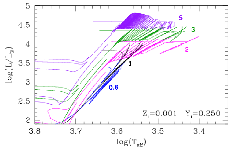
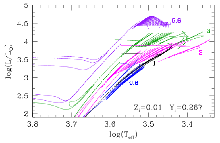
Figure 12: Selected evolutionary tracks of low- and intermediate-mass stars, zooming in their coolest and brighter parts in the H-R diagram, for different values of the stellar mass at the onset of the TP-AGB phase (indicated in $M_{\odot}$ nearby the corresponding track), and for two choices of the initial chemical composition. The plots include the entire TP-AGB tracks calculated with COLIBRI, and a portion of the previous evolution computed with PARSEC. Note the smooth transition from PARSEC to COLIBRI.

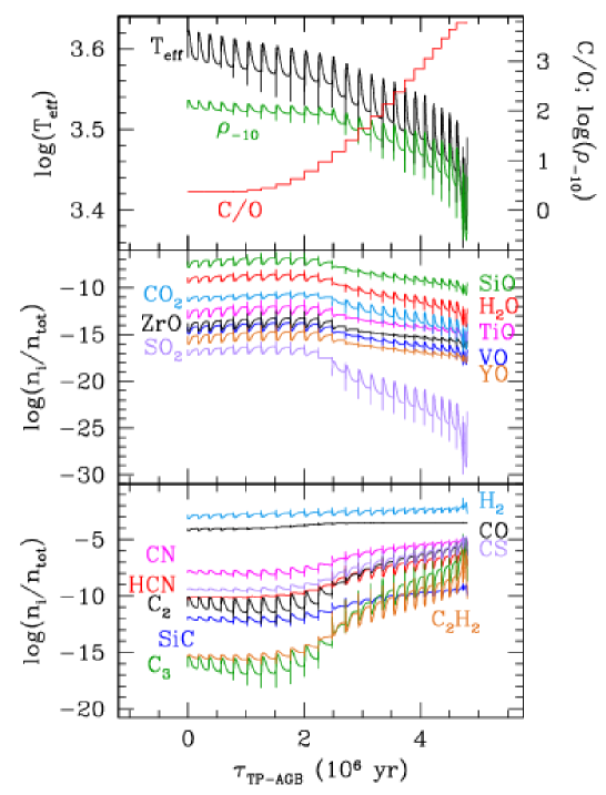
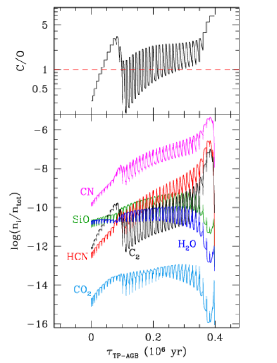
Figure 13: Left-hand side panel: Evolution of temperature, density, C/O ratio, and concentrations of the most abundant molecular species in the gas phase at the photosphere during the TP-AGB phase of a model with initial parameters $M_{\rm i}=2\,M_{\odot}$, $Z_{\rm i}=0.008$. The star experiences several third dredge-up events so that it is expected to become a carbon star. Note the huge dynamical range of the molecular concentrations, up to $\simeq 25$ orders of magnitude! Right-hand side panel: Evolution of the photospheric C/O ratio and concentrations of six selected molecular species, among the most abundant ones, during the whole TP-AGB phase of a model with initial parameters $M_{\rm i}=4\,M_{\odot}$, $Z_{\rm i}=0.0005$, experiencing both very deep third dredge-up and efficient HBB. Note the key role of the C/O ratio in governing the trends of the different molecules, as well as the several crossings at C/O$=1$.

For each PARSEC set of stellar tracks of given ($Z_{\rm i},Y_{\rm i}$) combination, we extract the initial conditions at the $1^{\rm st}$ TP for all the values of the initial stellar mass in the grid, ranging from $\simeq 0.5\,M_{\odot}$ to $M_{\rm up}$, the latter being the maximum mass for a star to develop an electron-degenerate C-O core. We deal typically with $60-70$ low- and intermediate-mass tracks for each initial chemical composition.

The core mass at $1^{\rm st}$ thermal pulse, $M_{\rm c,1}$, fixes a lower limit to the mass of the remnant white dwarf, and it is closely connected to the initial-final mass relation.

Figure 11 shows the PARSEC predictions for $M_{\rm c,1}$, as a function of the stellar mass for several choices of the initial metallicity. The stellar mass, $M_{1}$, is the value at the onset of the TP-AGB phase, so that, in principle, one should correct for the amount of mass lost by low-mass stars $(M_{\rm i}\la 2\,M_{\odot})$ during the red giant branch (RGB) phase in order to translate the $M_{\rm c,1}$ relation as a function of the initial stellar mass.

Two are the main features common to all the curves, namely: i) the almost constancy of $M_{\rm c,1}$ for stellar masses lower than $1.6-2.0\,M_{\odot}$ (depending on $Z_{\rm i}$), which simply reflects the fact that these stars develop He-cores of very similar mass due to the electron degeneracy after the main sequence; ii) the change of slope at stellar masses in the range $2.5-3.5\,M_{\odot}$ (depending on $Z_{\rm i}$) and the subsequent flattening of the $M_{\rm c,1}$ relations. This is the fingerprint of the occurrence of the second dredge-up during the Early-AGB of intermediate-mass stars, that causes a significant reduction of their core masses.

In Table 4 of Appendix A we present the fitting coefficients that we derive following the parametrization proposed by Wagenhuber & Groenewegen (1998), for several metallicities. In each panel of Fig. 11 the fitting curves are over-imposed to the PARSEC data for $M_{\rm c,1}$. We note, however, that our TP-AGB calculations use the true $M_{\rm c,1}$ values, and not those derived from the formulas.

6.2 TP-AGB evolution

For each stellar model with initial parameters $(M_{\rm i},Z_{\rm i})$ the characteristic quantities at the $1^{\rm st}$ thermal pulse (core mass, luminosity, effective temperature, envelope chemical composition), obtained from the PARSEC database, are fed as initial conditions to the COLIBRI code, which computes the TP-AGB evolution until when almost the entire envelope is lost by stellar winds. Operatively the COLIBRI calculations are stopped when the mass of the residual envelope falls below a limit of $0.002M_{\odot}-0.005M_{\odot}$. At this stage all evolutionary tracks are already evolving off the AGB towards higher effective temperatures, with a luminosity that depends mainly on the mass of the C-O core, and the phase of the pulse cycle at which the last event of mass ejection took place (see Fig 12).

For the present work we adopt a specific set of prescriptions for the mass loss and the third dredge-up, which we briefly outline below. These models will serve as a reference case for our ongoing TP-AGB calibration, and therefore the current parameters may be somewhat changed in future calculations. Anyhow, from various preliminary tests made with the present models, we expect that they already yield a fairly good description of the TP-AGB phase.

Mass loss.

It has been included under the hypothesis that it is driven by two main mechanisms, dominating at different stages. Initially, before radiation pressure on dust grains becomes the main agent of stellar winds, mass loss is described with the semi-empirical relation by Schröder & Cuntz (2005), which essentially assumes that the stellar wind originates from magneto-acoustic waves operating below the stellar chromosphere. The corresponding mass-loss rates are indicated with $\dot{M}_{\rm pre-dust}$.

Later on the AGB the star enters the dust-driven wind regime, which is treated with an approach similar to that developed by Bedijn (1988), and recently adopted by Girardi et al. (2010), to which the reader is referred for all details. Briefly, assuming that the wind mechanism is the combined effect of two processes, i.e., radial pulsation and radiation pressure on the dust grains in the outermost atmospheric layers, we adopt a formalism for the mass-loss rate as a function of basic stellar parameters, mass $M$ and radius $R$, expressed in the form $\dot{M}\propto e^{M^{a}R^{b}}$. The free parameters $a$ and $b$ have been calibrated on a sample of Galactic long-period variables with measured mass-loss rates, pulsation periods, stellar masses, radii, and effective temperatures. More details about the fit procedure will be given elsewhere. We denote the corresponding mass-loss rates with $\dot{M}_{\rm dust}$.

The key feature of this formalism is that it predicts an exponential increase of the mass-loss rates as the evolution proceeds along the TP-AGB, until typical super-wind values, around $10^{-5}-10^{-4}\,M_{\odot}{\rm yr}^{-1}$, are eventually reached. The super-wind mass loss is described in the same fashion as in Vassiliadis & Wood (1993), and corresponds to a radiation-driven wind, $\dot{M}_{\rm sw}=L/c\,v_{\rm exp}$, where $c$ is the speed of light and $v_{\rm exp}$ is the terminal velocity of the wind.

At any time during the TP-AGB calculations the actual mass-loss rate is taken as

$$\dot{M}={\rm max}[\dot{M}_{\rm pre-dust},{\rm min}(\dot{M}_{\rm dust},\dot{M}_{\rm sw})].$$ (25)

The third dredge-up.

The onset of the third dredge-up is predicted according to the scheme described in Sect. 3.6.1. The minimum temperature parameter is set to $\log(T_{\rm dup})=6.4$. This rather low value favours an early occurrence of the third dredge-up episodes. The efficiency $\lambda$ of the third dredge-up is computed with the analytic fits provided by Karakas, Lattanzio & Pols (2002), as a function of current stellar mass and metallicity.

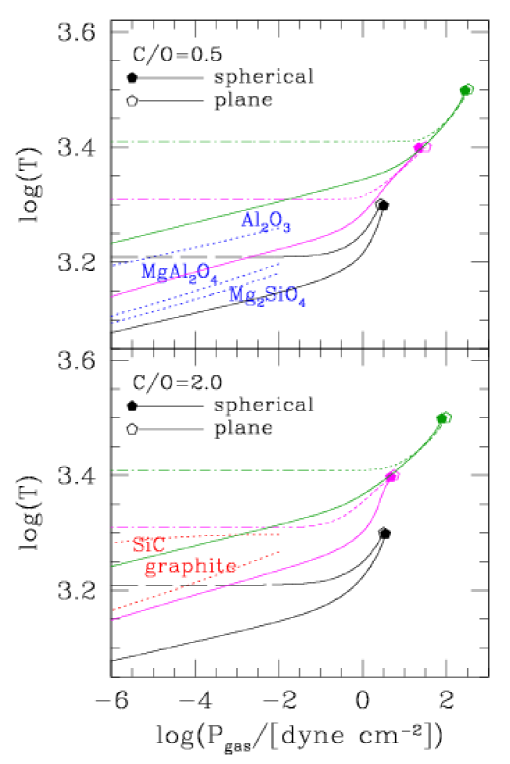
Figure 14: $P_{\rm gas}-T$ structure of static atmospheres corresponding to stellar model with $M=M_{\rm i}=1\,M_{\odot}$, $Z=Z_{\rm i}=0.008$, $X_{\rm i}=0.70$, $L=10^{4}\,L_{\odot}$, and three choices of the effective temperature, i.e. $\log(T_{\rm eff})=3.5,\,3.4,\,3.3$. The thermodynamic stratification is shown for both plane-parallel (dot-dashed line) and spherically symmetric (solid line) geometries, and assuming either C/O$=0.5$ (top panel), or C/O$=2.0$ (bottom panel). The photospheres are indicated by pentagons. The dotted lines correspond to the condensation temperatures at varying gas pressure for a few relevant species, namely: corundum (Al₂O₃), spinel (MgAl₂O₄), and forsterite (Mg₂SiO₄) as predicted by Lodders & Fegley (1999) for C/O$=0.5$ (top panel); graphite (C) and silicon carbide (SiC) from Lodders & Fegley (1995) for C/O$=2.0$.

Figure 12 illustrates a few selected evolutionary tracks of low- and intermediate-mass stars, zooming in their brightest portions in the H-R diagram, that include the whole TP-AGB computed with COLIBRI and some earlier evolution calculated with PARSEC. The transition from PARSEC to COLIBRI is not even distinguishable in most cases, except for the higher mass models with HBB ($M_{\rm i}=5.0M_{\odot},\,Z_{\rm i}=0.001$ and $M_{\rm i}=5.8M_{\odot},\,Z_{\rm i}=0.01$) for which COLIBRI predicts somewhat cooler effective temperature at the $1^{\rm st}$ TP compared to PARSEC. This difference has been discussed in Sect. 5.1, and can be partly explained in terms of the small differences in molecular opacities adopted by the two codes (see Fig. 6).

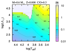
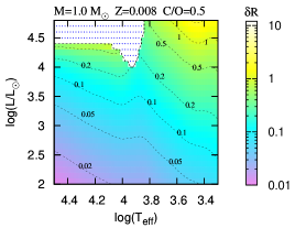
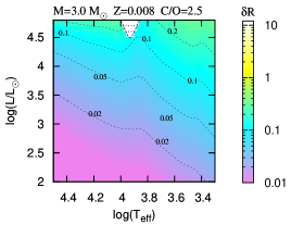
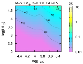
Figure 15: Maps of geometrical thickness $\Delta R$ of static stellar atmospheres in the H-R diagram, for four choices of the stellar mass and metallicity $Z_{\rm i}=0.008$, as indicated. The radial extension, defined by Eq. (7), is referred to the outermost radius at which $P_{\rm gas}$ has decreased to $10^{-4}$ dyne cm^-2. Contour lines of constant $\delta R$ (as indicated) are superimposed. The dotted regions correspond to unbound atmospheres, i.e. in which the radiative acceleration exceeds the gravitational acceleration somewhere between $R$ and $R_{0}$, so that the Eddington factor $\Gamma$ (Eq. 26) becomes larger than unity.

We also note in Fig. 12 that low-mass models ($M_{\rm i}=0.6M_{\odot},\,1.0M_{\odot}$) are characterised by quite narrow TP-AGB tracks since at given metallicity, as long as the surface C/O$<1$, the effective temperature is mostly determined by stellar mass and luminosity. Differently, models with larger masses ($M_{\rm i}=2.0M_{\odot},\,3.0M_{\odot}$), which are expected to undergo the transition to carbon stars, exhibit a pronounced displacement towards lower effective temperatures, mainly driven by the increase in molecular opacities. Finally, models with the highest masses ($M_{\rm i}=5.0M_{\odot},\,5.8M_{\odot}$) present TP-AGB tracks with the typical bell-shape modulated by the occurrence of HBB, and with the peak in luminosity reached when the envelope mass starts being drastically reduced by stellar winds. These considerations apply in general to both metallicity cases here considered ($Z_{\rm i}=0.001$ and $Z_{\rm i}=0.01$), with some systematic differences, i.e. lower effective temperatures are expected at higher metallicities, again due to surface opacity effects. A more detailed analysis of this aspect is given in Sect. 7.3.

Finally, we note that in our TP-AGB calculations no particular convergence problem was met all the way to the complete ejection of the envelope, whereas other studies, based on full TP-AGB calculations, report the divergence of the models in the late stages of evolution (e.g., Wood & Faulkner, 1986; Wagenhuber & Weiss, 1994; Lau et al., 2012). In the latter paper the authors suggest that the cause of the instability in the most massive TP-AGB models may be related to a local opacity maximum of Fe at the base of the convective envelope. At present we cannot identify the reason for the different behaviour of COLIBRI, this delicate point will deserve a closer look in follow-up studies.

7 Overview and analysis of the COLIBRI predictions

In the following we will discuss some relevant predictions of the COLIBRI code, with the aim of understanding a few key dependencies of the various physical processes at work and their complex interplay, as well as giving a general overview of the COLIBRI predictive capability.

7.1 Molecular concentrations at the photosphere

The on-the-fly use of the ÆSOPUS code during the TP-AGB calculations enables us to predict, for the first time, the evolution of the abundances of $\simeq 500$ molecular species in the outermost layers of the envelope. In Fig. 13 (left-hand side panel) we show the results at the photosphere of a $M_{\rm i}=2\,M_{\odot}$, $Z_{\rm i}=0.008$ model. We see clearly how the occurrence of thermal pulses produces large variations of the photospheric temperature and density (top panel), which in turn cause similar “pulses” in the concentrations of the molecules.

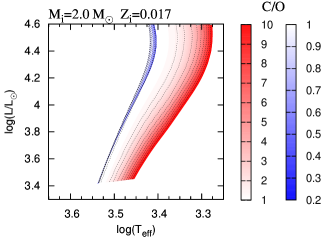
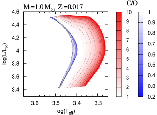
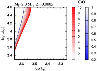
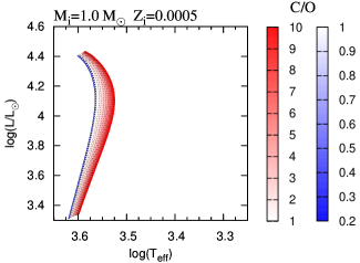
Figure 16: Hayashi lines on the AGB at increasing surface C/O ratio, color-coded according to the scales at the right-hand side of each plot, i.e. shades of blue for C/O$\leq 1$, shades of red for C/O$>1$. Results are shown for constant stellar mass, $M=1.0\,M_{\odot}$ and $M=2.0\,M_{\odot}$, and two choices of the initial metallicity $Z_{\rm i}=0.017$, and $Z_{\rm i}=0.0005$. Contour lines from C/O$=0.2$ to C/O$=10$, with an incremental step $\Delta$(C/O)$=0.2$, are superimposed to guide the eye. See the text for more details.

As amply discussed in Sects. 3.1 and 3.2 the other critical factor determining the molecular chemistry is the surface C/O ratio. The model under consideration experiences several third dredge-up episodes, that make the C/O ratio increase above unity (top panel). At the stage C/O$\approx 1$ we note an abrupt change in the molecular equilibria: while the abundances of the O-bearing molecules drop (middle panel), the C-bearing molecules suddenly start dominating the atmospheric chemistry (bottom panel). The abundance variations due to the increase of the C/O ratio are indeed remarkable, and they may span many orders of magnitudes! In this respect we also acknowledge the numerical stability of ÆSOPUS code, which is able to handle molecular species down to trace concentrations (e.g. SO₂ drops down to $\simeq 10^{-30}$ in the last TPs). At variance with the other molecules, the concentration of the carbon monoxide (CO) remains almost unperturbed by the evolution of the C/O ratio (except for a modest increment following the increase of C), due to its extremely large bond energy.

To better appreciate the role of the C/O ratio as the main driving factor of molecular chemistry, Fig. 13 (right-hand side panel) zooms in the evolution of just six molecules, among the most abundant ones, during the TP-AGB phase of a $M_{\rm i}=5\,M_{\odot}$, $Z_{\rm i}=0.001$ star. This model is predicted to suffer significant changes in its envelope chemical composition due to both the third dredge-up and HBB, which produce a complex evolution of the C/O ratio. We expect that the surface C/O follows a sawtooth trend crossing the critical region around unity several times, even during the single TPs. This may happen under particular conditions such that one dredge-up episodes brings the C/O$>1$ and later, during the interpulse period, HBB is able to burn C into N, hence lowering C/O below unity again.

In particular we note that the during the last TPs HBB is extinguished while the third dredge-up keeps on taking place, so that a significant increase of the C/O ratio is predicted in the last stages, as already noted by Frost et al. (1998). Correspondingly, the molecular species exhibit quite drastic variations: the C-bearing molecules (CN, HCN, C₂) follow the steep increase of the C/O ratio, whereas those of the O-bearing molecules (SiO, H₂O, CO₂) show a specular behaviour. Eventually the abundances of all molecules drop when the atmosphere starts warming up as the star evolves off the AGB.

7.2 Extended atmospheres in the H-R diagram

Figure 14 displays the gas pressure – temperature stratifications of a few static atmosphere models (with the same stellar mass and luminosity), under the assumption of either plane parallel or spherically-symmetric geometry (see Sect. 3.4). Computations were carried out for three values of the effective temperature and two choices of the C/O ratio.

It is interesting to note that, at least for the models under consideration, at given $T_{\rm eff}$ and C/O, the photospheric pressure is almost insensitive to the geometry, while the separation between the thin and the extended atmospheres grows wider and wider at lower pressures. On the contrary a major effect is produced by the C/O ratio: at fixed $T_{\rm eff}$, the photospheric pressure is lower for C-rich than for O-rich models. This will have a sizable impact on the inner envelope structure of AGB stars with different C/O ratios, since the photosphere sets two of the four boundary conditions for the envelope integrations described in Sect. 3.5.1.

By comparing the atmospheric structures for the two geometry options in Fig. 14, it is clear the relevance of the dilution of the radiation field in the extended atmospheres of AGB stars. For instance, for C/O$=2.0$ the plane-parallel model with $T_{\rm eff}\geq 3.4$ remains too cool and does not enter the condensation region of SiC and graphite, while the corresponding spherical model does it successfully. On the other hand, almost all models with C/O$=0.5$ stay outside the condensation area even at the lowest $T_{\rm eff}=3.3$. Indeed, a detailed analysis on the nucleation and growth of dust grains in the outer envelopes of AGB stars requires abandoning the static approximation in favour of an expanding envelope model. This important issue is beyond the scope of the present work, and is addressed in a forthcoming paper (Nanni et al., 2013).

Figure 15 illustrates the areas in the H-R diagram where AGB and post-AGB stars (cooler than $\sim 3\times 10^{4}$ K) are expected to have extended atmospheres, i.e. the radial extension of the atmosphere being a non-negligible fraction of the photospheric radius. The geometrical thickness $\delta R$ is defined according to Eq. (7).

First of all we note that, at given stellar mass, $\delta R$ increases at higher $L$ and lower $T_{\rm eff}$. Giants with lower masses have thicker atmospheres (higher $\Delta R$), since smaller $M/L$ values tend to reduce the effective gravitational acceleration, $g_{\rm eff}=(1-\Gamma)g$, by increasing the Eddington factor

$$\Gamma=\frac{\kappa}{4\pi Gc}\frac{L}{M}$$ (26)

where $g=GM/R^{2}$ is the gravitational acceleration, $\kappa$ is the flux-averaged opacity, while the other constants have their usual meanings. As shown in the top panels of Fig. 15, these conditions are preferably met by evolved M-type stars of low mass, a circumstance already discussed by e.g. Schmid-Burgk, Scholz & Wehrse (1981), and Laskarides & Nikolaidis (1990).

At higher $L$ and increasing $T_{\rm eff}$ atmospheres may even become gravitationally unbound, as the Eddington factor rises above unity due to the increasing opacity $\kappa$ in the outermost layers. In fact, for temperatures $\log(T)\ga 3.8$ K, the Rosseland mean opacity is expected to grow steeply due to the increasing contributions of the hydrogen bound-free and free-free absorptions (see e.g. Marigo & Aringer, 2009). It follows that this condition may apply, for instance, to post-AGB stars with high mass ($\ga\!1M_{\odot}$) (evolved from more massive AGB stars with HBB) on their way towards the hotter regions of the H-R diagram (see the dotted area top-right panel of Fig. 15).

7.3 Hayashi lines on the TP-AGB

Figure 16 displays several sequences of AGB Hayashi lines, with the aim of illustrating their basic dependencies on stellar mass, envelope mass, metallicity and C/O ratio. To this aim we consider two choices of the stellar mass, $1.0\,M_{\odot}$ and $2.0\,M_{\odot}$, and two values of the initial metallicity $Z_{\rm i}=0.0005,\,{\rm and}\,0.017$.

The surface C/O ratio is made vary from $0.1$ to $10$ in steps of $\Delta($C/O$)=0.2$, by increasing the C abundance, while keeping O constant (to mimic the effect of the third dredge-up). Therefore the actual metallicity $Z$ increases as C/O increases.

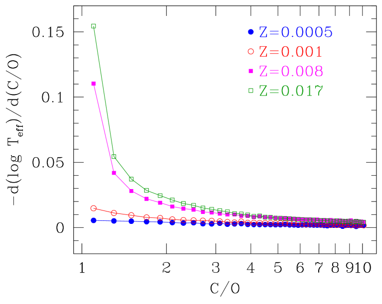
Figure 17: Cooling rate, measured by the derivative $|d(\log T_{\rm eff})/d({\rm C/O})|$, as a function of increasing C/O ratio (in the regime $>1$) as predicted by envelope integrations referring to a model with a mass of $2\,M_{\odot}$ and luminosity $\log(L/L_{\odot})=4$. Note the pronounced sensitivity to the initial metallicity.

For each value of C/O, the core mass $M_{\rm c}$ is made increase from $0.5\,M_{\odot}$ in steps of $\Delta M_{\rm c}=0.1\,M_{\odot}$, until either the luminosity reaches $\log(L/L_{\odot})=4.6$, or the envelope mass falls below $10\%$ of the total stellar mass, i.e. $(M-M_{\rm c})/M<0.1$. While the former condition is first met by the $2.0\,M_{\odot}$ sequences, the latter applies to the $1.0\,M_{\odot}$ tracks, that are terminated when $M_{\rm c}=0.94\,M_{\odot}$.

The effective temperature and the luminosity are determined by complete integrations of envelope models (see Sect. 3.5.1), with gas opacities calculated on-the-fly consistently with the current chemical composition (and C/O ratio).

We remark that these calculations are simply grids of envelope integrations and are meant to yield an overall picture of the Hayashi lines of C stars and their critical dependencies, but they cannot, by construction, be strictly representative of the TP-AGB evolution. For instance, the over-luminosity effect due to a deep third dredge-up is not taken into account and the Hayashi lines in Fig. 16 are those corresponding to a standard CMLR (for $\lambda=0$). As a consequence, at a given stellar mass, luminosity, and C/O ratio the “actual” effective temperature of an evolving C star model should be somewhat lower than that predicted in Fig. 16. This said, the following discussion is nevertheless instructive since the general trends remain valid.

Examining Fig. 16 several features can be noticed. As long as C/O$<1$ the Hayashi lines have a steep slope and span a limited $T_{\rm eff}$ range, which becomes narrower at decreasing metallicity. This interval defines the expected location of M and S stars. The value C/O$=1$ corresponds to the warmest Hayashi line, due to a deep minimum in the molecular opacities (nearly all C and O atoms are locked in the CO molecule; see Marigo & Aringer, 2009).

As soon as C/O overcomes unity we expect a sudden jump of the Hayashi lines to lower effective temperatures, the amplitude of the temperature jump being more pronounced at increasing metallicity. The cooling rate, expressed by the derivative $|d(\log T_{\rm eff})/d({\rm C/O})|$, progressively decreases at increasing C/O ratio, so that larger and larger C/O ratios are required to reach lower effective temperatures. This is evident by looking at the thickening of the iso-C/O curves in Fig. 16 (dashed lines), which become gradually closer one to the next.

It means that, above some critical C/O ratio, the atmospheric structure becomes less and less sensitive to a further increase of the carbon abundance. This kind of “saturation” effect shows up at lower C/O ratio for decreasing metallicity, as can be better appreciated in Fig. 17. We notice that at higher $Z_{\rm i}$ the cooling rate is large for C/O values slightly above $1$, then it decreases until it flattens out to a nearly constant, small value. This trend is found also at lower $Z_{\rm i}$, but with smoother features: the initial drop of $T_{\rm eff}$ becomes less pronounced and $|d(logT_{\rm eff})/d({\rm C/O})|$ levels off at lower C/O ratios. Note, for instance, the extremely low cooling rate at $Z_{\rm i}=0.0005$ all over the C/O ratio under consideration ($1\leq{\rm C/O}\leq 10$).

7.4 The core mass at the onset of the third dredge-up

As already mentioned in Sect. 3.6.1, we can determine the minimum core mass for the occurrence of the third dredge-up $M_{\rm c}^{\rm min}$, checking if and when the $T_{\rm bce}$ exceeds a critical value $T_{\rm dup}$ at the stage of post-flash luminosity peak. The quantity $T_{\rm dup}$ is assumed as a free parameter.

In Figure 18 the left-hand side panels display the $M_{\rm c}^{\rm min}$ predictions for $\log(T_{\rm dup})=6.2,6.4,6.5,6.6,6.7,6.8$ and three values of the initial metallicity, $Z_{\rm i}=0.02,\,Z_{\rm i}=0.008,\,{\rm and}\,Z_{\rm i}=0.004$. The numerical method described in Sect. 3.6.1 has been applied for stellar masses ranging from $1\,M_{\odot}$ to $3\,M_{\odot}$ in steps of $0.05\,M_{\odot}$. In practice, once set the minimum temperature $T_{\rm dup}$, for each initial stellar mass and chemical composition, $M_{\rm c}^{\rm min}$ is the value of the core mass for which $T_{\rm bce}=T_{\rm dup}$ is satisfied. The solution is found iteratively with envelope integrations adopting the Brent root-finding algorithm (chapter IX of “Numerical Recipes”; Press et al., 1988). In each case $M_{\rm c}^{\rm min}$ is taken as the maximum between the value obtained by the envelope-integration method and the core mass at the first thermal pulse, $M_{\rm c,1}$. We do not show the results for $M>3M_{\odot}$, since for the higher masses the temperature criterion is always satisfied since the onset of the TP-AGB, regardless of the value $T_{\rm dup}$. We see that all the curves share the same trend. Starting from lower masses towards the higher ones, $M_{\rm c}^{\rm min}$ slightly decreases, reaches a minimum and then steeply increases. It is interesting to note that the minimum in $M_{\rm c}^{\rm min}$ corresponds exactly to the critical maximum mass, $M_{\rm HeF}$, for a star to develop a degenerate He-core and experience the He-flash at the tip of the RGB. This reflects the same correspondence between $M_{\rm HeF}$ and the minimum of $M_{\rm c,1}$ (see Fig. 11), already pointed out long ago by Lattanzio (e.g. 1986).

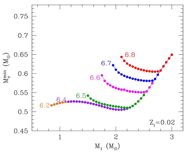
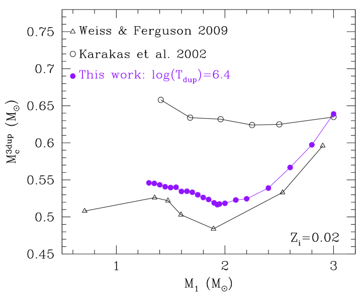
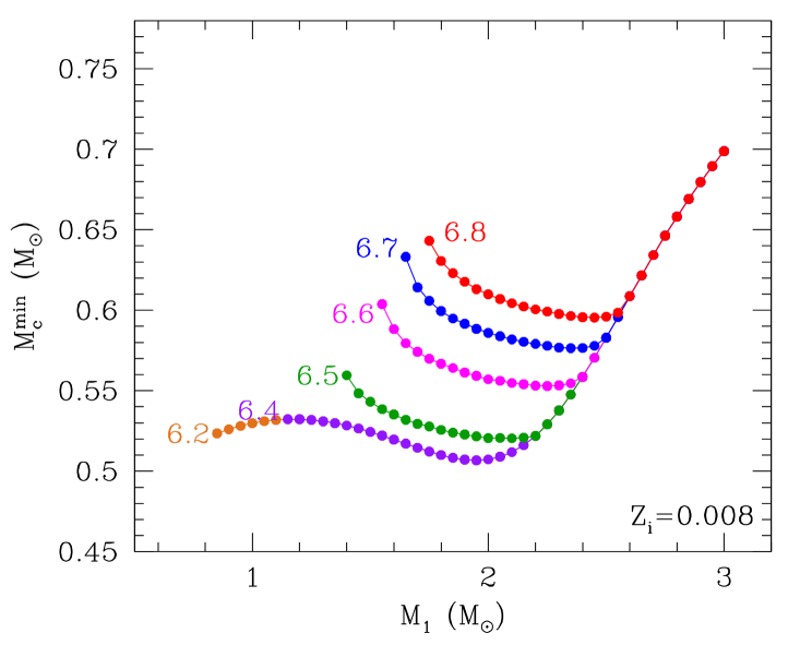
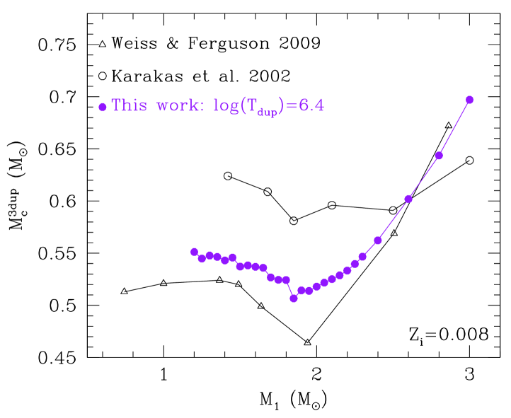
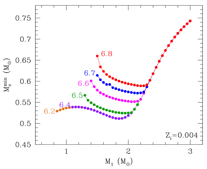
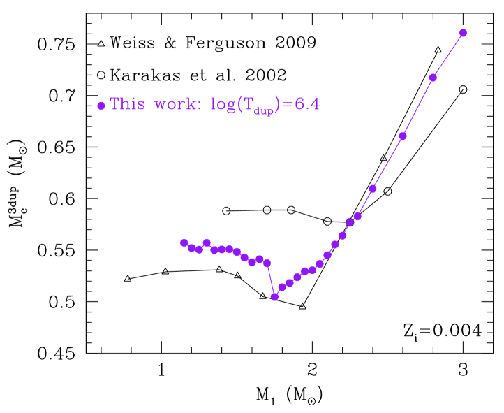
Figure 18: The minimum core mass for the third dredge-up as a function of the stellar mass at the onset of the TP-AGB phase, and three values of the initial metallicity as indicated. Left-hand side panels: Predictions for $M_{\rm c}^{\rm min}$ are obtained from envelope integrations, as detailed in Sect. 3.6.1, adopting six values of the minimum temperature for the base of the convective envelope, namely: $\log(T_{\rm dup})=6.2,6.3,6.4,6.5,6.6,6.7,6.8$. Right-hand side panels: The core mass at the first occurrence of the third dredge-up, $M_{\rm c}^{\rm 3dup}$, during the TP-AGB evolution of models of different masses and metallicities, as indicated. We compare the results from two sets of full TP-AGB calculations (Weiss & Ferguson, 2009; Karakas, Lattanzio & Pols, 2002), with the COLIBRI predictions assuming $\log(T_{\rm dup})=6.4$.

For a given initial metallicity, at decreasing $T_{\rm dup}$, the sequences move downward and reach lower stellar masses, that is $M_{\rm c}^{\rm min}$ decreases and the third dredge-up is expected to take place in stars of lower and lower masses. We note that for $T_{\rm dup}\leq 6.4$ the minimum core mass $M_{\rm c}^{\rm min}$ coincides with $M_{\rm c,1}$.

The values of the core mass, $M_{\rm c}^{\rm 3dup}$, when the third dredge-up effectively occurs for the first time during the TP-AGB evolution, are shown in the right-hand side panels of Figure 18. We note that, in general, $M_{\rm c}^{\rm 3dup}\geq M_{\rm c}^{\rm min}$, as expected. The COLIBRI results for $M_{\rm c}^{\rm 3dup}$, corresponding to $\log(T_{\rm dup})=6.4$, show a similar trend with the stellar mass compared to full TP-AGB models calculations. At the same initial metallicity and stellar mass our predictions for $\log(T_{\rm dup})=6.4$ are lower than Karakas, Lattanzio & Pols (2002), but somewhat larger than Weiss & Ferguson (2009).

Clearly significant differences exist between the two sets of full calculations, which supports the need to accurately calibrate $M_{\rm c}^{\rm min}$ with the aid of observations of M and C giants of different ages and metallicities. This calibration is presently underway and will be presented in subsequent papers.

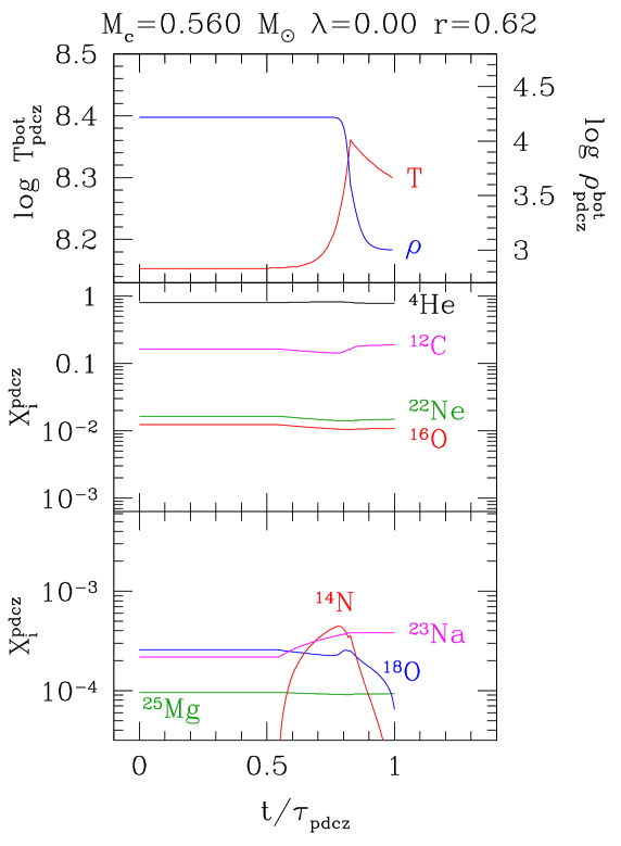
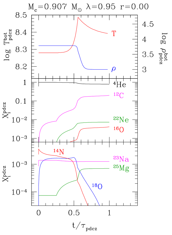
Figure 19: Structural characteristics of the pulse-driven convective zone, corresponding to the $10^{\rm th}$ and $18^{\rm th}$ thermal pulse of the $M_{1}=1.2\,M_{\odot},\,Z_{\rm i}=0.017$ (left panel) and $M_{1}=5.4\,M_{\odot},\,Z_{\rm i}=0.017$ (right panel) models, respectively. The corresponding values of the core mass ($M_{\rm c}$), efficiency of the third dredge-up ($\lambda$), and degree of overlap ($r$) are indicated on top of each plot. Quantities are presented as a function of the phase $\phi=t/\tau_{\rm pdcz}$, from the onset of pulse convection ($\phi=0$) to its disappearance ($\phi=1$). For each stellar model, the panels show the evolution of temperature and density at the current PDCZ base (top panel); the evolution of the PDCZ abundances (in mass fractions), homogenized over the current PDCZ mass (middle and bottom panels).

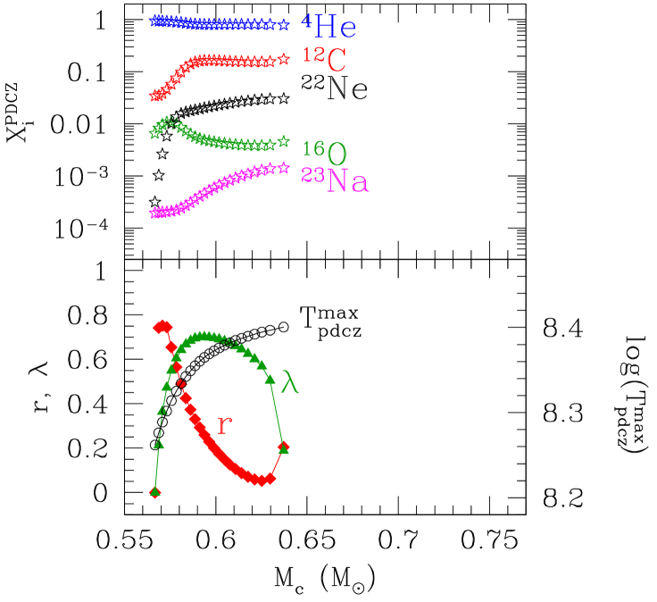
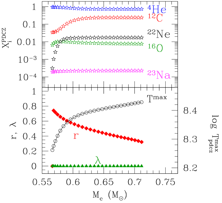
Figure 20: Top panels: predicted intershell abundances as a function of the core mass during the entire TP-AGB phase of a ($M_{\rm i}=2.6,\,Z_{\rm i}=0.017$) model. Bottom panels: Evolution of the maximum temperature $T^{\rm max}$ reached at the bottom of the PDCZ at each TP, efficiency $\lambda$ of the third dredge-up, and degree of overlap $r$ between two consecutive PDCZs. The results in the right-hand side panels are obtained under the assumption that the third dredge-up does not occur ($\lambda=0$). Note that in this case the ²³Na abundance in the PDCZ is lower than in models with dredge-up (left-hand side panel).

7.5 Intershell abundances

The standard chemical composition of the intershell region, left after the development of a thermal pulse, amounts to roughly $20\%-25\%$ of ¹²C, $1\%-2\%$ of ¹⁶O, $1\%-2\%$ of ²²Ne, with ⁴He essentially comprising all the rest (Schönberner, 1979; Boothroyd & Sackmann, 1988b; Mowlavi, 1999a), almost regardless of metallicity and core mass.

These standard values are presently debated. Izzard et al. (2004) find a lower value for ¹⁶O, typically amounting to $\approx\,0.5\%$, while the inclusion of convective diffusive overshooting applied to all convective boundaries of the PDCZ determines a substantial increase of the ¹²C and ¹⁶O abundances at the expense of ⁴He (Herwig et al., 1997). Herwig (2000) shows that with his calibrated parametric scheme for overshoot, the ¹²C and ¹⁶O intershell abundances reach typical values of $0.45$, and $0.25$, respectively.

We will now discuss our predictions obtained from the semi-analytic scheme detailed in Sect. 3.6.2. Figure 19 exemplifies the evolution of the main characteristics of the PDCZ during a thermal pulse, in two models with different core masses. Let us first analyse the results for the model with $M_{\rm c}=0.576\,M_{\odot}$ (left-hand side panels).

We see that while the density at the bottom of the PDCZ is continuously dropping, the corresponding temperature first rises up to the maximum value, $T_{\rm pdcz}^{\rm max}$, and then decreases (top panels).

Before reaching the maximum temperature, the chemical composition of the PDCZ may vary mainly due to its growth in mass, as the ashes of the H-burning shell are reached by the expanding convection. As a consequence the abundances of ⁴He, ¹⁴N, and ²³Na are expected to increase. The sharp rise of ¹⁴N is evident in the bottom left-hand side panel of Fig. 19. The increase of ¹⁴N is only temporary: as soon as the PDCZ heats up nitrogen is completely destroyed by the chain ${}^{14}{\rm N}(^{4}{\rm He},\gamma)^{18}{\rm F}(\beta^{+}\nu)^{18}{\rm O}$.

In the short phase around the temperature maximum the PDCZ reaches its widest mass extension. At this point the main $\alpha$-capture reactions are turned on, leading to the production of primary carbon via the $\rm\,{}^{4}\kern-0.8pt{He}\,({2\,^{4}He}\,,{\gamma})\,{}^{12}\kern-0.8pt{C}\,$ reaction, together with some synthesis of ¹⁶O from $\rm\,{}^{12}\kern-0.8pt{C}\,({{}^{4}He}\,,{\gamma})\,{}^{16}\kern-0.8pt{O}\,$, and ²²Ne from $\rm\,{}^{18}\kern-0.8pt{O}\,({{}^{4}He}\,,{\gamma})\,{}^{22}\kern-0.8pt{Ne}\,$. Correspondingly the ⁴He abundance decreases.

Finally, when the PDCZ cools and the convection recedes the chemical composition barely changes, so that the entire intershell with mass $\Delta M_{\rm pdcz}$ is assigned the final mixture at $\phi=1$.

Basically the same analysis holds for the model with the higher core mass (right-hand side panels), but for a few differences that are explained mainly by the higher $T_{\rm pdcz}^{\rm max}$, the shorter duration $\tau_{\rm PDCZ}$ of the PDCZ, and by the previous dredge-up history. As we discuss later, the intershell abundances do depend on the indirect interaction of one pulse with the preceding one, which can be quantified by the so-called “degree of overlap”, denoted with $r$. We also note that in the model with higher $M_{\rm c}$ a higher $T_{\rm pdcz}^{\rm max}$ is attained so that $\rm\,{}^{22}\kern-0.8pt{Ne}\,({{}^{4}He}\,,{n})\,{}^{25}\kern-0.8pt{Mg}\,$ is also activated. This reaction is recognized as a source of neutrons for the s-process nucleosynthesis in more massive AGB stars (e.g. Busso, Gallino & Wasserburg, 1999; Pumo et al., 2009).

Figure 20 shows the evolution of the final PDCZ abundances left after each thermal pulse (bottom panels), during the entire TP-AGB evolution of the ($M_{\rm i}=2.6,\,Z_{\rm i}=0.017$) model. The left- and right-hand side panels compare the results in the cases the third dredge-up takes place (left-hand side panel; $\lambda>0$) or does not (left-hand side panel; $\lambda=0$). In the $\lambda>0$ case, the efficiency of the third dredge-up is described following the analytic relations presented by Karakas, Lattanzio & Pols (2002) which fit the results of their full AGB models (see also Sect. 6.2), the $\lambda=0$ case is simply treated setting the efficiency to zero at each thermal pulse. This is equivalent to assume a high value for $T_{\rm dup}$. Several remarks can be made.

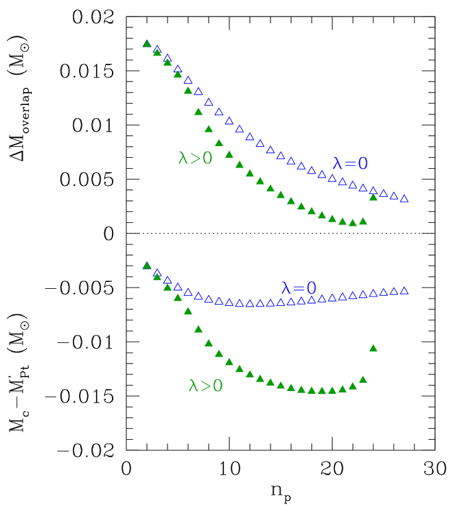
Figure 21: Mass of overlap, $\Delta M_{\rm overlap}$, between two consecutive PDCZs, and mass difference $(M_{\rm Pt}^{\prime}-M_{\rm c})$ between the top of the previous PDCZ, $M_{\rm Pt}^{\prime}$, and the current core mass, $M_{\rm c}$. Predictions are shown as a function of the pulse number, for the same evolutionary sequences of Fig. 20, computed with two different assumptions for the efficiency third dredge-up: $\lambda=0$ (empty blue triangles), or $\lambda>0$ (filled green triangles; according to the relations of Karakas, Lattanzio & Pols (2002)). Note the effect of the third dredge-up that pushes $M_{\rm Pt}^{\prime}$ inward.

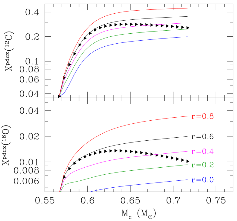
Figure 22: Dependence of the intershell abundances of ¹²C (top panel) and ¹⁶O (bottom panel) on the degree of overlap $r$ between consecutive PDCZs. The bunch of lines show the predictions for a constant value of $r$ (indicated in the bottom panel) between consecutive PDCZs. The sequences of triangles show the PDCZ abundances as a function of the core mass during the evolution of a TP-AGB star with ($M_{\rm i}=2.6M_{\odot},\,Z_{\rm i}=0.017$) in which we assume the third does not occur. In this test case the TP-AGB phase is computed without mass loss to extend the calculations up to $M_{\rm c}=0.7\,M_{\odot}$.

The “standard” intershell abundances.

Our intershell abundances of ⁴He, ¹²C, and ¹⁶O recover nicely the “standard” values obtained by the class of full AGB models (e.g. Schönberner, 1979; Boothroyd & Sackmann, 1988b; Izzard et al., 2004; Karakas & Lattanzio, 2007) in which the borders of the PDCZ are determined by the classical Schwarzschild criterion applied to the temperature gradients. We find typical values of $\approx 20\,\%$ for ¹²C and $\approx 0.5\%-1\,\%$ for ¹⁶O (Figs. 20, 22, 24, 25). More specifically, our predictions for ¹⁶O are in closer agreement with the lower abundances reported by Izzard et al. (2004), than the higher values of $1\%-2\%$ defining the “standard” intershell composition (Boothroyd & Sackmann, 1988b). This difference will be discussed below, being likely related to the efficiency of the third dredge-up.

Dependence on the degree of overlap.

The degree of overlap $r$ is defined as the fraction of the matter contained in a given PDCZ that is incorporated into the PDCZ produced at the next thermal pulse. The reader may refer to Table 2 for the operative definition of $r$ in terms of mass coordinates, and to Fig. 3 for a graphical representation. The parameter $r$ was originally introduced and discussed in early studies (e.g. Ulrich, 1973; Iben, 1975; Truran & Iben, 1977; Iben, 1977) to highlight the importance of the overlap between successive pulses to the slow-neutron capture nucleosynthesis of heavy elements, especially in relation to the synthesis of ²²Ne and its role in the release of neutrons via the $\rm\,{}^{22}\kern-0.8pt{Ne}\,({{}^{4}He}\,,{n})\,{}^{25}\kern-0.8pt{Mg}\,$ reaction.

We also find a significant dependence of the intershell abundances on the degree of overlap $r$ between consecutive PDCZs. This can be better appreciated by looking at the bottom panels of Fig. 20. We see that the degree of overlap tends in general to decrease from pulse to pulse, but the occurrence of the third dredge-up ($\lambda>0$) makes $r$ to drop more steeply, eventually reaching zero in the last TPs. The smooth decline of $r$, expected for $\lambda=0$, is mostly due to the inverse correlation between $\Delta M_{\rm pdcz}$ and $M_{\rm c}$ (see top panel of Fig. 5), so that less massive PDCZs are produced in later TPs. On the other hand, every time a dredge-up event takes place the upper border, $M_{\rm Pt}$, of the PDCZ is shifted inward in mass coordinate, by an amount which is larger at increasing $\lambda$. This circumstance causes a further reduction of $r$. We find that for $\lambda\ga 0.7$ the overlap $r\simeq 0$, implying that the PDCZs are almost decoupled one from the next.

This effect is clearly shown in Fig. 21, where the mass difference, $M_{\rm Pt}-M_{\rm c}$, becomes more and more negative when the third dredge-up is active ($\lambda>0$), at variance with the nearly constancy, or even small increase, expected if the process does not take place ($\lambda=0$). Consequently, the decrease of the overlap mass between two consecutive PDCZs, $\Delta M_{\rm overlap}$, is steeper at increasing $\lambda$. We note that in the TP-AGB model with $\lambda>0$ the overlap mass gradually reduces to almost zero, and then it grows again in the very last thermal pulses when the third dredge-up does not take place anymore.

The consequences on the PDCZ nucleosynthesis are exemplified in Fig. 20. While in absence of dredge-up events $(\lambda=0)$ all intershell abundances tend to flatten out at nearly constant values, when the third dredge-up takes place this pattern is modified. In particular, as the third dredge-up starts to occur we expect that the intershell abundance of ¹⁶O somewhat declines levelling off in the last TPs, while those of ²²Ne and ²³Na increase, steadily. These findings for ²²Ne and ²³Na are in full agreement with Mowlavi (1999a, b), to which the reader should also refer for a very detailed analysis.

The increase of ²²Ne, that reaches up to $\simeq 2\%-3\%$ in the cases under consideration, is directly related to the increase of primary ¹²C in the envelope composition caused by the third dredge-up. The more abundant the surface ¹²C is, the larger amount of ¹⁴N is synthesized during the interpulse period by the CNO-cycle operating in the radiative H-burning shell. In turn, the more abundant ¹⁴N is, the more ²²Ne will be produced by the chain of reactions ${}^{14}{\rm N}(^{4}{\rm He},\gamma)^{18}{\rm F}(\beta^{+}\nu)^{18}{\rm O}(^{4}{\rm He},\gamma)^{22}{\rm Ne}$ occurring inside the PDCZ.

The increase of ²³Na is related to the larger envelope abundance of ²²Ne, that we expect as a consequence of the third dredge-up. We recall that the ²³Na in the PDCZ is not synthesized in situ during the pulse, but is it inherited as part of the material processed by the radiative H-burning shell, where the conversion ${}^{22}{\rm Ne}(p,\gamma)^{23}{\rm Na}$ took place.

The trends of the ¹²C and ¹⁶O intershell abundances, mainly synthesized as primary products during the TPs, are also affected by the third dredge-up, hence by the degree of overlap between consecutive PDCZs.

To better investigate this aspect, we have performed a few test calculations, assuming each time a different value of the overlap parameter $r$, which is kept constant along a pre-determined sequence of thermal pulses. Given a selected value of $\widehat{r}$, at each thermal pulse the mass coordinate of the top of the previous PDCZ, $M_{\rm pdcz}^{\prime}$, is artificially varied such that the condition $\Delta M_{\rm overlap}=M_{\rm Pt}^{\prime}-M_{\rm He}=\widehat{r}\,\Delta M_{\rm pdcz}$ is fulfilled (see Fig. 3). This is equivalent to suitably adjusting the maximum depth of the third dredge-up, hence its efficiency $\lambda$.

The results are presented in Fig. 22, together with a TP-AGB sequence computed without the third dredge-up (black triangles). From the intersections with the bunch of lines we can read out the corresponding values of the degree of overlap $r$, which is found to decrease slowly from roughly $0.8$ to $0.4$.

As for the PDCZ abundances, we notice that, after the first pulses, the curves tracing the evolution of the intershell abundances at constant $r$, run almost parallel at increasing core mass. For instance, at $M_{\rm c}=0.65\,M_{\odot}$, passing from $r=0.8$ to $r=0.0$ the ¹²C (¹⁶O) concentration decreases from $\simeq 41\,\%$ ($\simeq 2.7\,\%$) to $\simeq 17\,\%$ ($\simeq 0.5\,\%$). The relative change with $r$ appears larger for ¹⁶O ($approx$ a factor of six) than for ¹²C ($approx$ a factor of two).

From these results we suggest that the lower ¹⁶O intershell abundances ($<1\%$) reported by Izzard et al. (2006), compared to the standard values ($1\%-2\%$) found by Boothroyd & Sackmann (1988b) reflect the larger efficiency of the third dredge-up (i.e. higher $\lambda$ hence lower $r$) found in the more recent works compared to the past.

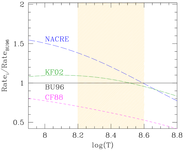
Figure 23: Comparison of a few versions for the ${}^{12}{\rm C}(^{4}{\rm He},\gamma)^{16}{\rm O}$ rate, taken from the JINA reaclib database (Cyburt et al., 2010). They correspond to Caughlan & Fowler (1988, CF88), Angulo (1999, NACRE), Buchmann (1996, BU96), Kunz et al. (2002, KF02). We plot the ratio of each rate relative to BU96, which is our default choice. The hatched area corresponds to the relevant range of the temperature attained at the bottom of the PDCZ (see Fig. 5).

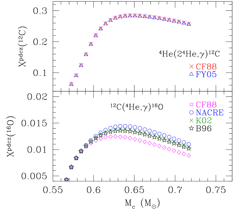
Figure 24: Dependence of the intershell abundances of ${}^{12}{\rm C}$ (top panel) and ${}^{16}{\rm O}$ (bottom panel) on the nuclear reaction rates $\rm\,{}^{4}\kern-0.8pt{He}\,({2\,^{4}He}\,,{\gamma})\,{}^{12}\kern-0.8pt{C}\,$, and $\rm\,{}^{12}\kern-0.8pt{C}\,({{}^{4}He}\,,{\gamma})\,{}^{16}\kern-0.8pt{O}\,$, respectively. Labels in the top panel stand for the Caughlan & Fowler (1988, CF88) and the Fynbo et al. (2005, FY05) rates, while labels in the bottom panel are the same as in Fig. 23. The calculations refer to the same TP-AGB model with ($M_{\rm i}=2.6,\,Z_{\rm i}=0.017$), as in Fig. 22.

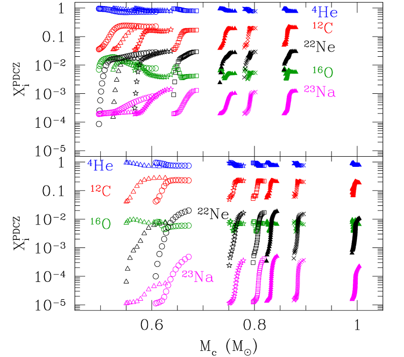
Figure 25: Predicted intershell abundances as a function of the core mass overt the entire TP-AGB evolution for a few models with various choices of the initial mass ($1.2\,M_{\odot}$: empty triangles; $2.0\,M_{\odot}$: empty circles; $2.6\,M_{\odot}$: stars; $3.0\,M_{\odot}$: empty squares; $4.0\,M_{\odot}$: crosses; $2.0\,M_{\odot}$: filled triangles. The initial metallicity is $Z_{\rm i}=0.017$ (top panel) and $Z_{\rm i}=0.001$ (bottom panel).

Dependence on the nuclear reaction rates.

We have investigated the robustness of the “standard” intershell composition against reasonable changes in two key nuclear reaction rates, namely ${}^{4}{\rm He}(2\,^{4}{\rm He},\gamma)^{12}{\rm C}$ and ${}^{12}{\rm C}(^{4}{\rm He},\gamma)^{16}{\rm O}$. A few versions for the latter rate are compared in Fig. 23. The results for the PDCZ abundances of ${}^{12}{\rm C}$ and ${}^{16}{\rm O}$ are shown in Fig. 24. There is an almost perfect overlap of the ¹²C predictions obtained with the Caughlan & Fowler (1988) and the Fynbo et al. (2005) rates. This is not surprising since the two versions are quite similar (with a relative difference always below $1\%$) in the temperature range of interest for the pulse nucleosynthesis, i.e. $2\times 10^{8}{\rm K}\la T\la 4\times 10^{8}{\rm K}$.

The results for ¹⁶O exhibit a somewhat larger dependence, but still modest, on the assumed ${}^{12}{\rm C}(^{4}{\rm He},\gamma)^{16}{\rm O}$. A comparison of four rates for this reaction is displayed in Fig. 23. In the relevant temperature range the largest difference reaches roughly a factor of $2$ between the Caughlan & Fowler (1988) and the Fynbo et al. (2005) rates, while the variation in the intershell abundance of ¹⁶O remain quite small, $\approx 10\%$. The rather low sensitivity of the ¹⁶O abundance PDCZ to significant changes of the ${}^{12}{\rm C}(^{4}{\rm He},\gamma)^{16}{\rm O}$ rate was already noticed by Boothroyd & Sackmann (1988b) and is essentially explained by the fact that the proper temperature conditions are kept for too short a time to allow a sizable conversion of ${}^{12}{\rm C}$ into ¹⁶O.

Dependence on stellar mass and metallicity.

Figure 25 shows the evolution of the final PDCZ abundances left after each thermal pulse, during the entire TP-AGB evolution of models with a few values of initial stellar masses and two choices of the initial metallicity $Z_{\rm i}=0.017$ and $Z_{\rm i}=0.001$. As already mentioned, our predictions are essentially consistent with the recent results from full stellar models without overshooting applied to the PDCZ (Mowlavi, 1999a; Karakas, Lattanzio & Pols, 2002; Izzard et al., 2004). In particular the ¹²C abundance evolves towards an asymptotic value of $\simeq 20\%$, independent of mass and metallicity, while in most cases the ¹⁶O abundance settles down around a value of $\simeq 0.005-0.008$, in any case lower than $2\%$ reported by Boothroyd & Sackmann (1988b).

The abundance of ²²Ne is nearly always larger than that of ¹⁶O, reaching up to $\approx 2\%-3\%$ in models with $Z_{\rm i}=0.017$, while lower values up to $\approx 1\%-2\%$ are attained for $Z_{\rm i}=0.001$. However we note that, relative to its value at the first TP, the PDCZ concentration of ²²Ne shows a larger increase in lower metallicity models, while at larger metallicity the increment is by one order of magnitude at most. This result is likely related to the fact that at lower metallicity we expect a more efficient enrichment of primary ¹²C, hence of the total CNO abundance, in the envelope caused by the third dredge-up. In this way the synthesis of ²²Ne is favoured, as it is the end product of a chain of $\alpha$-capture reactions that just start with ¹⁴N, the most abundant product of the CNO cycle (after ⁴He) operating in the H-burning shell.

A similar trend characterizes the evolution of the ²³Na intershell abundance, which depends on the proton capture reactions occurring in the H-burning shell during the quiescent interpulse periods. High-metallicity models show, in general, higher values of ²³Na ingested in the PDCZ, up to $\simeq 10^{-3}$, but the relative increase over the TP-AGB evolution is larger in low-metallicity models.

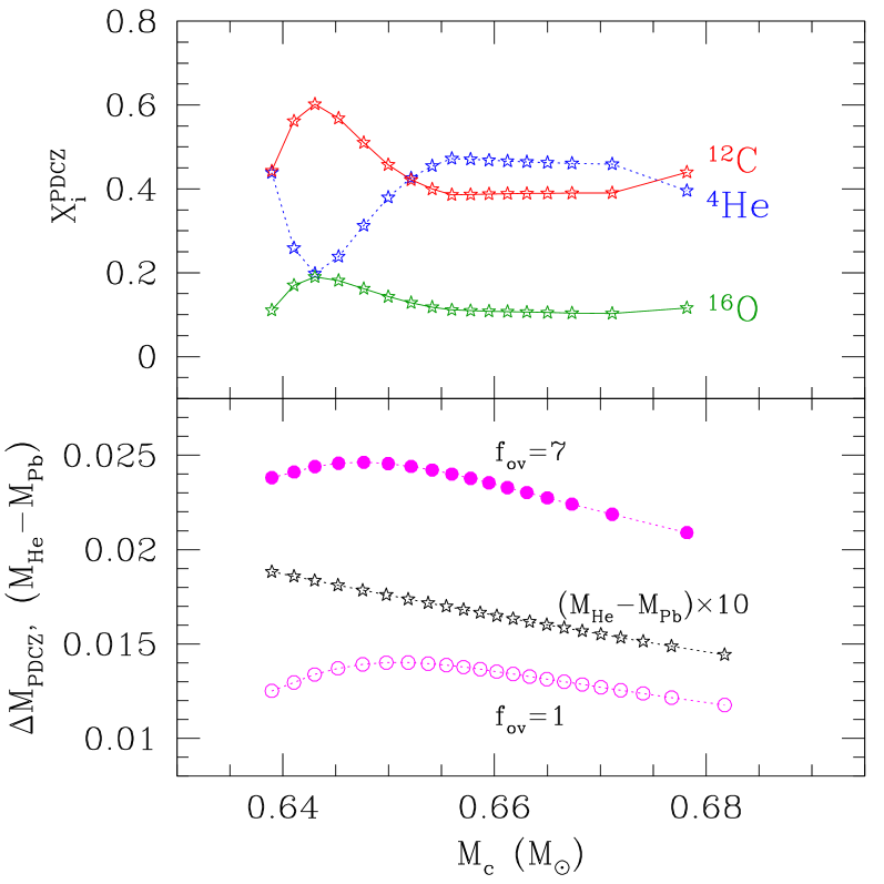
Figure 26: Top panel: PDCZ abundances as a function of the core mass at each TP of a model with initial mass $M_{\rm i}=3\,M_{\odot}$ and metallicity $Z_{\rm i}=0.02$. Predictions are obtained with a parameter $f_{\rm ov}=7$ that mimics the inclusion of convective overshoot at the base of the PDCZ. This value of $f_{\rm ov}$ allows to nicely reproduce the results of detailed calculations by Herwig (2000) for the same $(M_{\rm i},Z_{\rm i})$ combination. Bottom panel: Mass of the PDCZ at its maximum extension predicted with $f_{\rm ov}=1$ (empty circles), and with $f_{\rm ov}=7$ (filled circles). The amount of helium burning products ingested by the PDCZ, corresponding to the mass difference $(M_{\rm He}-M_{\rm Pb})$, multiplied by a factor of ten, is also shown. All masses are in solar units. See the text for more explanation.

Dependence on overshoot.

The scheme depicted in Fig. 3 for the PDCZ can be easily modified to account for overshoot applied to the base of the convective pulse. As a test case, we have considered the results obtained by Herwig (2000), who applied an exponential diffusive overshoot at the convective boundaries of the PDCZ. One major consequence is a depletion of helium and enhancement of carbon and oxygen in the intershell abundance distribution. Typical abundances (by mass) are $0.4-0.5$ for ¹²C, $0.15-0.20$ for ¹⁶O, and $0.30-0.40$ for ⁴He, obtained by Herwig (2000) with his calibrated overshoot parameter.

We underline that in our model the physical structure of the PDCZ is described via analytic fits to the results of full TP-AGB model (see Sect. 3.6.2), so that we cannot perform physical tests of stability against convection at the borders of the convective intershell. Nonetheless, we can simulate the effect of different prescriptions with the aid of a simple parametric approach. To mimic the effect of overshoot applied to the PDCZ boundaries, we shift inward the mass coordinate of its bottom, adopting the parametrization:

$$M_{\rm Pb}^{\rm oversh}=M_{\rm He}-f_{\rm ov}(M_{\rm He}-M_{\rm Pb})\,,$$ (27)

where $f_{\rm ov}\geq 1$ is an adjustable factor. For $f_{\rm ov}=1$ we recover the typical intershell chemical composition that is predicted by full TP-AGB models when using the Schwarzschild criterion, while the effect of convective overshoot is simulated adopting $f_{\rm ov}>1$. As mentioned by Herwig (2000), there is no noticeable effect of overshoot at the top of the PDCZ, so that we keep the mass coordinate $M_{\rm Pt}$ unchanged.

The mass difference ($M_{\rm He}-M_{\rm Pb}$), derived from full TP-AGB calculations as a function of the core mass, is plotted in Fig. 26. We find that Herwig (2000) results are reasonably well reproduced with $f_{\rm ov}\simeq 7$, in terms of both PDCZ mass and abundances (see his figures 7d and 11 for the $(M_{\rm i}=3M_{\odot},Z_{\rm i}=0.02)$ model).

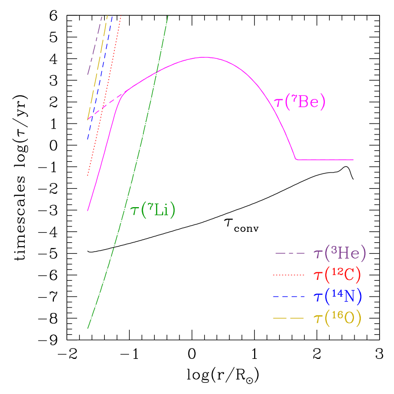
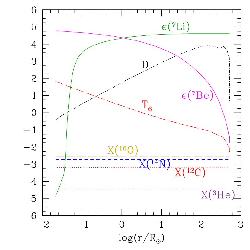
Figure 27: Thermodynamic and abundance profiles across the deep convective envelope of an intermediate-mass TP-AGB model experiencing HBB, with $M_{\rm i}=5.4\,M_{\odot}$ and $Z_{\rm i}=0.008$, taken at its maximum ⁷Li surface enrichment, when $M_{\rm bol}=-6.48$ and $M_{\rm c}=0.96\,M_{\odot}$. Left panel: Nuclear timescales of a few relevant species against proton captures and electron captures (only for ⁷Be), and convective timescale $\tau_{\rm conv}$. Right panel: Logarithmic profiles of abundances for a few selected species, expressed either in mass fraction (for ³He, ¹²C, ¹⁴N, ¹⁶O), or with the spectroscopic notation $\epsilon_{i}=\log[n_{i}/n({\rm H})]+12$, where $n$ corresponds to the number density of atoms (for ⁷Li and ⁷Be). The temperature $T_{6}=\log(T/10^{6}{\rm K})$ and the diffusion coefficient $\log(D/R_{\odot}^{2}\,{\rm yr}^{-1})$, defined by Eq. (20), are also shown.

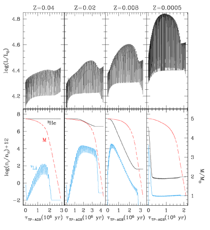
Figure 28: Hot-bottom burning and synthesis of lithium via the Cameron-Fowler beryllium transport mechanism in TP-AGB models with initial mass $M_{\rm i}=5\,M_{\odot}$ and varying metallicity. Top panel: Evolution of the luminosity during the TP-AGB phase. Note the larger HBB over-luminosity at decreasing metallicity. Bottom panel: Evolution of the surface abundances of ⁷Li, ³He, and of the current stellar mass being reduced by stellar winds.

Without pretending to investigate in more detail complex aspects of the PDCZ nucleosynthesis (e.g. the formation of the ¹³C pocket is not considered here), we underline that this simple parametric approach may be useful to explore the impact of the overshoot option on the formation and evolution of carbon stars, by comparing population synthesis simulations including overshoot with observations, an important test which is still to be done to our knowledge. An example of test calculation is discussed in the next Sect. 7.6, and illustrated in Fig. 29.

7.6 Hot-bottom burning nucleosynthesis

Figure 27 demonstrates the importance of including a time-dependent convective diffusion algorithm to treat the synthesis of lithium in intermediate-mass AGB stars with HBB. As thoroughly discussed by Sackmann & Boothroyd (1992), such an approach is necessary when the usual instantaneous mixing approximation is no longer valid. This is the case for nuclei, like ⁷Li and ⁷Be, whose lifetimes may become shorter or comparable to the convective timescale in some parts of the convective envelope. The circumstance $\tau_{\rm conv}\approx\tau_{\rm nuc}$ occurs in the inner regions for ⁷Li, and in the external layers for ⁷Be (see Fig. 27, left panel). As a consequence, the abundances of these species may vary considerably across the convective envelope, at variance with the concentrations of other nuclei (e.g. ³He, C, N, O) made homogeneous by the rapid convective mixing.

In particular, the convective envelopes of intermediate-mass AGB stars present the suitable thermodynamic conditions to put the Cameron-Fowler beryllium transport mechanism (Cameron & Fowler, 1971) at work: ⁷Li is efficiently produced and sustained in the outermost layers by electron captures on ⁷Be nuclei until either the reservoir of ³He (involved in the reaction $\rm\,{}^{4}\kern-0.8pt{He}\,({{}^{3}He}\,,{\gamma})\,{}^{7}\kern-0.8pt{Be}\,$) is exhausted, or HBB is extinguished due to envelope ejection by stellar winds.

The model displayed in Fig. 27 shows the envelope structure of a TP-AGB star with $M_{\rm i}=5.4,\,Z_{\rm i}=0.008$, that may be considered as representative of the most luminous M giants in the Large Magellanic Cloud. The structure is taken at the maximum surface Li enrichment corresponding to $\epsilon(^{7}{\rm Li})\simeq 4.6$, and $M_{\rm bol}\simeq-6.5$, in nice agreement with the luminosities and the highest measured values of Li in the LMC super-rich Lithium stars (Smith & Lambert, 1989, 1990; Smith et al., 1995). Note the mirror behaviours of ⁷Be and ⁷Li abundances: towards the surface ⁷Li is efficiently produced by electron captures on ⁷Be nuclei.

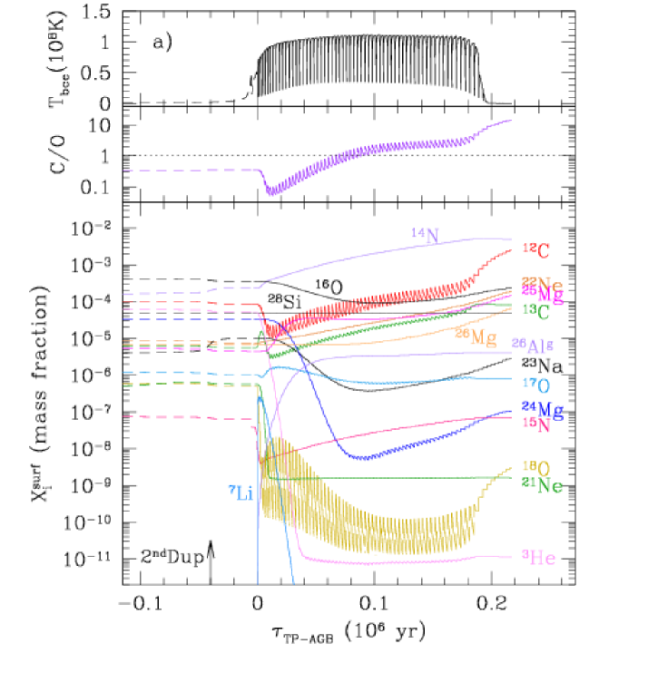
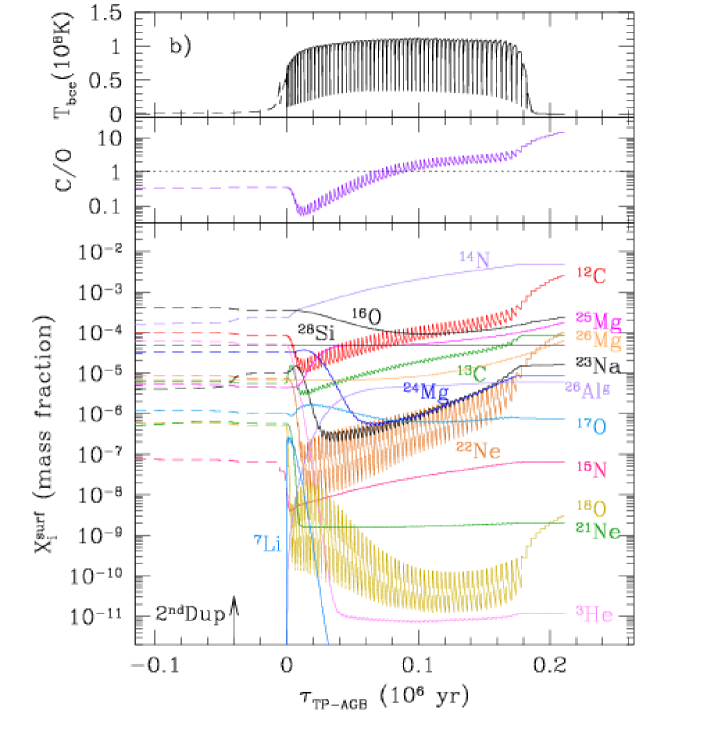
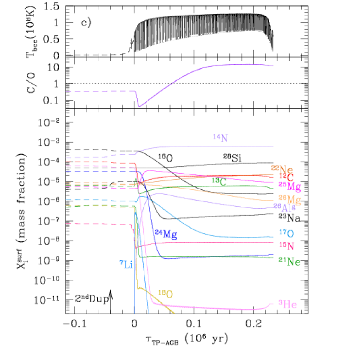
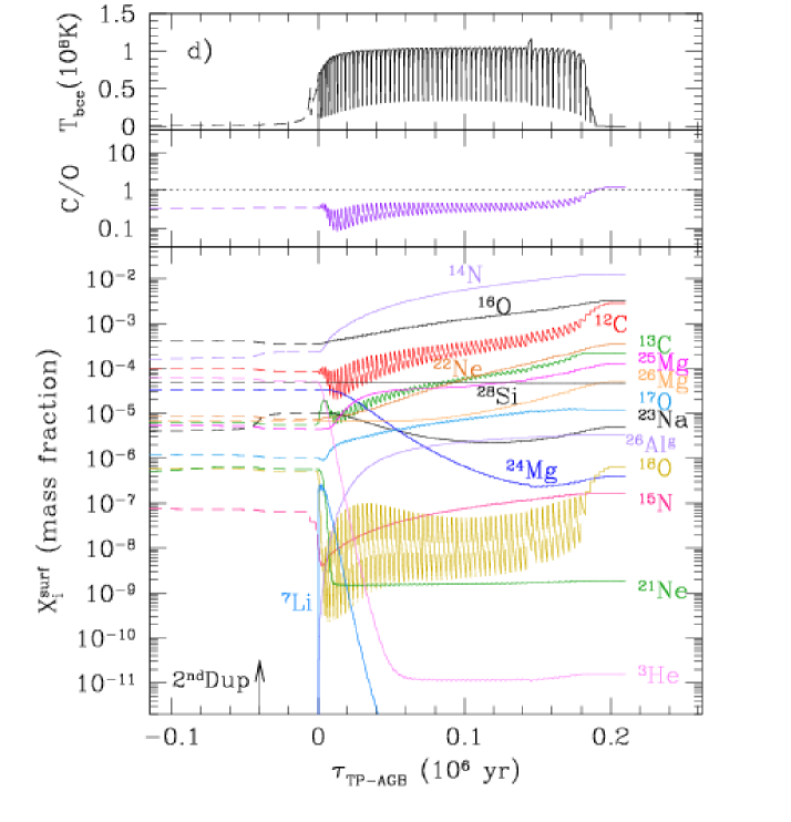
Figure 29: Evolution of the temperature at the base of the convective envelope, surface C/O ratio and elemental abundances during the whole TP-AGB phase of a $M_{\rm i}=5\,M_{\odot},Z_{\rm i}=0.001$ model (solid lines) computed with the COLIBRI code. The nucleosynthesis of all species is coupled in time and in space with a diffusive description of convection. Time is counted since the first TP. We show also a portion of the previous evolution (negative times) during the early-AGB predicted by the PARSEC stellar evolution code (dashed lines). The arrow indicates the approximate stage at which the second dredge-up takes place. Panel a) corresponds to the reference model computed with the default set of prescriptions, while panels b), c), and d) show the results obtained changing selected parameters. Panel b: different rates for the nuclear reactions $\rm\,{}^{22}\kern-0.8pt{Ne}\,({p}\,,{\gamma})\,{}^{23}\kern-0.8pt{Na}\,$, $\rm\,{}^{23}\kern-0.8pt{Na}\,({p}\,,{\gamma})\,\kern-0.8pt{\,{}^{4}He+^{20}\kern-2.0pt{Ne}}\,$, and $\rm\,{}^{23}\kern-0.8pt{Na}\,({p}\,,{\gamma})\,{}^{24}\kern-0.8pt{Mg}\,$ (corresponding to the “ths8” version of the JINA REACLIB database). Panel c: suppression of the third dredge-up ($\lambda=0$). Panel d: carbon- and oxygen-enhanced chemical composition of the intershell. Note that the nucleosynthesis is not computed via a post-process technique (i.e. assuming a fixed temperature and density stratification), but in all cases the chemical and thermodynamic structure of the envelope is solved at each time step throughout the TP-AGB phase.

Figure 28 compares the evolution of luminosity and surface ⁷Li abundance in TP-AGB stars with the same initial mass of $5M_{\odot}$ but different metallicities. A few points are worth noting. Since at decreasing $Z$ higher temperatures at the base of the envelope are reached, the brightening of stars with HBB along the TP-AGB becomes steeper at lower metallicity, so that the classical Paczyński limit (Paczyński, 1970), at $M_{\rm bol}~{}\simeq-7.1$, may be even exceeded, like the $M_{\rm i}=5M_{\odot},\,Z_{\rm i}=0.0005$ model does. In fact, because of the break-down of the CMLR in stars with HBB, the Paczyński limit is no longer a true upper bound to the AGB luminosity (Blöcker & Schönberner, 1991; Boothroyd & Sackmann, 1992), so that AGB stars brighter than $M_{\rm bol}~{}\simeq-7.1$ could be effectively be observed with a core mass $M_{\rm c}<1.4\,M_{\odot}$.

At the same time, the synthesis of lithium is more efficient at lower metallicity due to the larger amounts of ⁷Be produced in the innermost layers of the envelope by the $\rm\,{}^{4}\kern-0.8pt{He}\,({{}^{3}He}\,,{\gamma})\,{}^{7}\kern-0.8pt{Be}\,$ reaction. But for very high metallicities, e.g. $Z_{\rm i}=0.04$, at which the Li production remains quite modest (left-hand side panels of Fig. 28), in the other cases under consideration a maximum value around $\log[n(^{7}{\rm Li})/n({\rm H})]+12\simeq 4-4.5$ is reached, that is only moderately dependent on $Z_{\rm i}$. This limiting value is in full agreement with earlier computations by Sackmann & Boothroyd (1992), and it is the result of the high temperature sensitivity of $\tau(^{7}{\rm Be})$ from one side, and of similar temperature conditions for the maximum Li synthesis in envelope models, on the other side.

Finally, we note that there should be a limited range of metallicity for which we expect AGB stars to contribute to the lithium enrichment of the interstellar medium. Comparing the trends of the ⁷Li abundance and the current stellar mass (bottom panels of Fig. 28), we see that for only models with $Z_{\rm i}=0.02$ significant mass loss takes place when the surface ⁷Li is high, while at higher and lower metallicities, the ejecta are practically ⁷Li free. In fact at $Z_{\rm i}=0.04$ the ⁷Li synthesis is just a small and short-lived event, whereas at $Z_{\rm i}=0.008$ and $Z_{\rm i}=0.0005$ the ⁷Li production is quite efficient but confined to the earliest stages of the AGB evolution, so that when the super-wind regime of mass loss is attained, practically whole ⁷Li has been destroyed, following the progressive exhaustion of the ³He reservoir. These conclusions are drawn for a particular set of stellar models, while a more general analysis should be extended also to other values of the stellar mass, which will be done a future investigation.

Figure 29 exemplifies the results of the nucleosynthesis calculations made by COLIBRI over the entire TP-AGB evolution of a $M_{\rm i}=5.0,\,Z_{\rm i}=0.001$ model, corresponding to a low-metallicity star experiencing strong HBB.

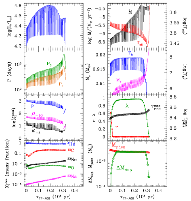
Figure 30: Sample output provided by the COLIBRI code. The evolution of several quantities, over the whole TP-AGB phase, is shown for a $(M_{\rm i}=5\,M_{\odot},\,Z_{\rm i}=0.008)$ model, which may be taken as representative of the most luminous M-giants in the LMC. The entire TP-AGB evolution, consisting of 48 thermal pulse cycles, has been calculated in roughly $40$ minutes, using a standard 2.2 GHz CPU. Each quantity is quoted with either [n] or [a], depending on whether it is predicted by numerical integrations of envelope models and/or nuclear networks, or it is derived from analytic fitting relations. From top-left to bottom-right the eight panels show the evolution of (i) surface luminosity $L$ [n], (ii) mass-loss rate $\dot{M}$ [a] and effective temperature $T_{\rm eff}$ [n], (iii) fundamental and first-overtone pulsation periods $P_{0},\,P_{1}$ [a], (iv) core mass $M_{\rm c}$ [n] and temperature at the base of the convective envelope $T_{\rm bce}$ [n], (v) photospheric values of pressure $P$ [n], density $\rho_{-10}=\rho/(10^{-10}\,{\rm gr\,cm}^{-3})$ [n], and Rosseland mean opacity $\kappa_{-4}=\kappa/10^{-4}$ [n]: (vi) efficiency $\lambda$ [a] of the third dredge-up, maximum temperature $T_{\rm pdcz}^{\rm max}$ [a] at the bottom of the pulse-driven convective zone, and degree of overlap $r$ [n] between consecutive zones; (vii) inter-shell abundances [n]; (viii) mass of the pulse-driven convective zone $\Delta M_{\rm pdcz}$ [a], and dredged-up mass $M_{\rm Dup}$ [a] at each thermal pulse.

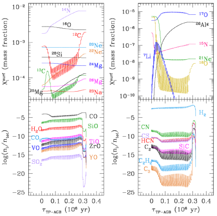
Figure 31: The same as in Fig. 30, but referred to chemical properties at the photosphere. Top panels: evolution of the surface abundances [n] of several light elements, modulated by the occurrence of the third dredge-up and HBB. For all species HBB nucleosynthesis is followed by coupling the nuclear network to a diffusive description of convection. Bottom panels: evolution of the photospheric concentrations of few molecular species [n] (O-bearing species on the left, C-bearing species on the right), which play a major role in determining the spectral features of AGB stars. Predictions are obtained with on-the-fly ÆSOPUS computations for the molecular chemistry, consistently coupled with the varying envelope abundances. Note the abrupt change in the molecular pattern over the very last TPs, when the surface C/O increases from below to above unity as a consequence of the third dredge-up.

The nucleosynthesis of the CNO, NeNa and MgAl cycles at low metallicities is of particular interest, in relation to the possible role of primordial AGB (and Super-AGB) stars as polluters of the gas out of which the old stars, presently observed in Galactic Globular Clusters (GGCs), may have formed (Ventura & D’Antona, 2008; Pumo, D’Antona & Ventura, 2008). In this so-called self-enrichment scenario the HBB nucleosynthesis in metal-poor AGB (and Super-AGB) stars could have left its signatures in the prominent chemical anti-correlations (C-N, O-Na, Mg-Al) currently detected in GGC stars (Carretta et al., 2009).

Indeed, our COLIBRI code may be fruitfully employed to investigate the several debated issues about the AGB chemical yields in the low $Z$ regime. An example is given in Fig. 29, where we compare the results of four sets of computations obtained with exactly the same set of parameters, but varying a few key assumptions that should sample the spread in the predictions of current TP-AGB models. The effects on the predicted evolution of several light elements is remarkable. The results of our reference model, computed with the default set of input prescriptions, are shown in panel a) of Fig. 29.

In the first test case (panel b), we have changed the rates of three nuclear reactions, namely $\rm\,{}^{22}\kern-0.8pt{Ne}\,({p}\,,{\gamma})\,{}^{23}\kern-0.8pt{Na}\,$, $\rm\,{}^{23}\kern-0.8pt{Na}\,({p}\,,{\gamma})\,\kern-0.8pt{\,{}^{4}He+^{20}\kern-2.0pt{Ne}}\,$, and $\rm\,{}^{23}\kern-0.8pt{Na}\,({p}\,,{\gamma})\,{}^{24}\kern-0.8pt{Mg}\,$, replacing those quoted in Table 1 with the theory rates labeled “ths8” in the JINA REACLIB database, that were calculated with the NON-SMOKER code^WEB version 5.0w developed by T. Rauscher and presented in Cyburt et al. (2010). At the typical temperatures $T_{\rm bce}\ga 10^{8}$ K, the “ths8” rates are higher than the default ones. In particular, the “ths8” destruction rate $\rm\,{}^{22}\kern-0.8pt{Ne}\,({p}\,,{\gamma})\,{}^{23}\kern-0.8pt{Na}\,$ can be larger by up to 3 orders of magnitude! The large impact is evident by comparing the abundance trends of ²²Ne, ²³Na, and ²⁴Mg in panels a) and b).

In the second test case (panel c), we assume that no third dredge-up takes place, i.e. $\lambda=0$ at each TP, a condition found, for instance, in the recent models of super-AGB stars by Siess (2010), where the absence of extra-mixing at the edge of the convective boundaries prevents the development of dredge-up episodes. The evolution of the elemental abundances in the envelope is simply regulated by the CNO, NeNa, and MgAl cycles. A very significant depletion of ¹⁶O is responsible for the transition to C/O$>1$. At the same time we see that, compared to the other models, the lack of carbon enrichment in the envelope favours the attainment of higher base temperatures $T_{\rm bce}$.

In the third test case (panel d), we mimic the effect of convective overshoot at the bottom of the PDCZ following the scheme described in Sect. 7.5. As a consequence, the intershell abundance distribution becomes carbon- and oxygen-enhanced compared to the classical composition, resembling the findings by Herwig (2000) (see Fig. 26). The differences with respect to the standard model shown in panel a) are sizable. The enrichment of ¹⁶O due to the third dredge-up prevails over the its destruction by HBB, producing a continuously increasing surface abundance of ¹⁶O. The C/O ratio remains lower than one for most of the TP-AGB evolution. Moreover, we note that the large increase of the metallicity due to the very efficient third dredge-up contributes to reach lower temperature $T_{\rm bce}$.

8 Closing remarks

8.1 Summary of COLIBRI’s features

In this paper we have presented the main improvements and novelties characterizing the COLIBRI code for the computation of the TP-AGB phase. They are briefly recalled below.

Compared to purely synthetic TP-AGB codes, COLIBRI relaxes a significant part of their analytic formalism in favour of a detailed physics which, applied to a complete envelope model, allows to predict self-consistently:

• the effective temperature, and more generally the convective envelope and atmosphere structures, suitably coupled to the changes in the surface chemical abundances and gas opacities;

• the CMLR and its possible break-down due to the occurrence of HBB in the most massive AGB stars, by taking properly into account the nuclear energy generation in the H-burning shell and in the deepest layers of the convective envelope;

• the HBB nucleosynthesis via the solution of a complete nuclear network coupled to a diffusive description of mixing, in which the current stratifications of temperature and density are derived from integrations of complete envelope models;

• the intershell abundances left by each thermal pulse via the solution of a complete nuclear network applied to a simple model of the pulse-driven convective zone;

• the onset and quenching of the third dredge-up, with a temperature criterion that is tested, at each thermal pulse, with the aid of envelope integrations at the stage of the post-flash luminosity peak.

At the same time COLIBRI pioneers new techniques in the treatment of the physics of stellar interiors, not yet adopted in full TP-AGB models. Compared to present-day full stellar evolutionary codes, the prerogatives of COLIBRI are related to 1) the computation of the equation of state and opacities, and 2) computation requirements, as below summarized.

• COLIBRI is able to perform the first ever on-the-fly accurate computation of the equation of state for roughly 800 atoms, ions, molecules, and of the Rosseland mean opacities throughout the atmosphere and the deep envelope. This has been accomplished by incorporating the ÆSOPUS code (Marigo & Aringer, 2009) and the Opacity Project software package (Seaton, 2005) as internal routines of the COLIBRI code. Avoiding the preliminary preparation of static tables and their subsequent interpolations, the new approach assures a complete consistency, step by step, of both EoS and opacity with the evolution of the chemical abundances caused by the third dredge-up and HBB. For the first time we show the evolution of the photospheric molecular concentrations during the TP-AGB phase, and their modulation driven not only by changes in the chemical compositions but also by the periodic occurrence of the TPs.

• Flexibility and optimized computation requirements. COLIBRI is competitive in terms of low computing-time requests. Tests made with a standard 2.2 GHz CPU processor have shown that COLIBRI, on average, computes one complete pulse-cycle in ${0.5-1.0}$ min against the ${60-90}$ min taken by full evolution codes, e.g. PARSEC (Bressan et al., 2012), with a gain factor of ${\approx\,100}$. This characteristic makes COLIBRI an agile tool suitable to carry out extensive calculations of the TP-AGB evolutionary tracks covering large and dense grids of stellar masses and metallicities.

Figures 30 and 31 collect a representative sample of the most significant quantities that can be predicted by COLIBRI throughout the entire TP-AGB evolution of a star with given initial mass and chemical composition. The quantity of available information is indeed large, including both structural and chemical properties. We plan to keep the same level of richness also in the stellar isochrones we are going to construct from the COLIBRI tracks.

8.2 Ongoing and planned applications

It should be mentioned that the present set of TP-AGB models is a preliminary release, since we are currently working to a global TP-AGB calibration as a function of stellar mass and metallicity, aimed at reproducing a large number of AGB observables at the same time (star counts, luminosity functions, C/M ratios, distributions of colors, pulsation periods, etc.) in different star clusters and galaxies. Since the calibration is still ongoing the current parameters (e.g. efficiency of the third dredge-up and mass loss) of the TP-AGB model may be changed in future calculations.

Anyhow, various tests indicate that the present version of the COLIBRI models already yields a fairly good description of the TP-AGB phase. Compared to our previously calibrated sets (Marigo & Girardi, 2007; Marigo et al., 2008; Girardi et al., 2010) the new TP-AGB models yield somewhat shorter, but still comparable, TP-AGB lifetimes, and they successfully recover various observational constraints dealing with e.g. the Galactic initial–final mass relation (Kalirai et al., in prep.), spectro-interferometric determinations of AGB stellar parameters (Klotz et al., 2013), the correlation between mass-loss rates and pulsation periods, and the trends of the effective temperature with the C/O ratio observed in Galactic M, S and C stars.

Further important support comes from the results of our new model for the condensation and growth of dust grains in the outflows of AGB stars (Nanni et al., 2013), which has been applied to the COLIBRI TP-AGB tracks. The results are extremely encouraging as they are found to nicely reproduce other independent sets of key observations, i.e. the correlation between expansion velocities and mass-loss rates/pulsation periods of Galactic AGB stars.

Appendix A Fitting relations

A.1 Properties of the pulse-driven convection zone

Here we present relations for characteristic quantities of the PDCZ, based on full TP-AGB calculations by Wagenhuber (1996); Karakas, Lattanzio & Pols (2002); Karakas & Lattanzio (2007). All masses are expressed in solar units, $\tau_{\rm pdcz}$ is given in years, and $T_{\rm pdcz}^{\rm max}$ in Kelvin degrees, $Z_{\rm i}$ denotes the initial metallicity.

$$\log(\tau_{\rm pdcz}) = a_{1}+a_{2}Z_{\rm i}+(a_{3}+a_{4}Z_{\rm i})M_{\rm c}$$

$$+10^{\displaystyle(a_{5}+a_{6}M_{\rm c}+a_{7}\Delta M_{\rm c,nodup})}$$

$$\log(T_{\rm pdcz}^{\rm max}) = (b_{1}+b_{2}\log(Z_{\rm i}))+(b_{3}+b_{4}\log(Z_{\rm i}))M_{\rm c}$$

$$-10^{\displaystyle(b_{5}+b_{6}\Delta M_{\rm c,nodup})}$$

$$\log(\rho_{\rm pdcz}^{\rm max})={\rm max}(3.7,c_{1}+c_{2}Z_{\rm i}+c_{3}M_{\rm c})$$ (30)

$$\log(\Delta M_{\rm pdcz}) = d_{1}+d_{2}M_{\rm c}+d_{3}M_{\rm c}^{2}+d_{4}\log(Z_{\rm i})$$

$$-10^{\displaystyle(d_{5}+d_{6}M_{\rm c}+d_{7}\Delta M_{\rm c,nodup})}$$

$$+d_{8}M_{\rm c}\log(Z_{\rm i})$$

$$x_{q}=\tau_{\rm q}/\tau_{\rm pdcz} = (e_{1}+e_{2}Z_{\rm i})M_{\rm c}+e_{3}Z_{\rm i}+e_{4}$$

$$-10^{\displaystyle(e_{5}M_{\rm c,1}+e_{6}\Delta M_{\rm c,nodup})}$$

A.2 The core mass at the $1^{\rm st}$ thermal pulse

We follow the parametrization proposed by Wagenhuber & Groenewegen (1998), where $M$ denotes the stellar mass at the onset of the TP-AGB phase. All masses are expressed in solar units. Coefficients are obtained by fitting the predictions from the PARSEC sets of stellar models (Bressan et al., 2012).

$$M_{\rm c,1} = [-p_{1}(M-p_{2})^{2}+p_{3}]f$$

$$+(p_{4}M+p_{5})(1-f)\,,$$

$$f = \left(1+{\rm exp}^{\frac{M-p_{6}}{p_{7}}}\right)^{-1}$$

Table 3: Fitting coefficients of analytic relations for a few key properties of the pulse-driven convection zone.

Eq. (A.1): PDCZ duration
$a_{1}$	$a_{2}$	$a_{3}$	$a_{4}$	$a_{5}$	$a_{6}$	$a_{7}$
4.675	-18.56	3.793	22.65	-2.451	2.216	116.7
Eq. (A.1): PDCZ maximum temperature
$b_{1}$	$b_{2}$	$b_{3}$	$b_{4}$	$b_{5}$	$b_{6}$
8.037	-0.06876	0.5697	0.07701	-0.8459	-22.18
Eq. (30): PDCZ maximum density
$c_{1}$	$c_{2}$	$c_{3}$
4.96	- 2.4	- 1.25
Eq. (A.1): PDCZ maximum mass
$d_{1}$	$d_{2}$	$d_{3}$	$d_{4}$	$d_{5}$	$d_{6}$	$d_{7}$	$d_{8}$
-1.134	0.2884	-1.898	-0.08295	-2.171	1.429	-21.55	0.09189
Eq. (A.1): Ratio of the quenching time over PDCZ duration
$e_{1}$	$e_{2}$	$e_{3}$	$e_{4}$	$e_{5}$	$e_{6}$
0.8220	0.9602	5.481	- 0.4321	-0.8632	-26.23

Table 4: Fitting coefficients of Eq. (A.2) for the core mass at the $1^{\rm st}$ thermal pulse.

$Z_{\rm i}$	$p_{1}$	$p_{2}$	$p_{3}$	$p_{4}$	$p_{5}$	$p_{6}$	$p_{7}$
0.0005	9.616573E-02	1.300268E+00	5.567979E-01	9.204736E-02	5.204188E-01	1.947073E+00	1.607459E-01
0.001	1.173875E-01	1.188889E+00	5.505528E-01	9.301397E-02	5.100448E-01	1.954574E+00	1.670251E-01
0.004	1.074609E-01	1.150773E+00	5.389349E-01	9.559346E-02	4.645270E-01	2.170495E+00	1.949511E-01
0.006	9.772655E-02	1.148381E+00	5.347831E-01	9.128342E-02	4.641443E-01	2.254396E+00	2.278098E-01
0.008	9.020493E-02	1.156664E+00	5.318839E-01	8.671702E-02	4.719326E-01	2.319841E+00	2.560683E-01
0.01	7.480933E-02	1.193024E+00	5.300704E-01	9.499056E-02	4.257837E-01	2.365426E+00	2.470678E-01
0.014	7.496712E-02	1.189756E+00	5.286927E-01	9.300582E-02	4.175395E-01	2.375119E+00	2.651535E-01
0.017	6.956924E-02	1.227015E+00	5.275279E-01	8.479260E-02	4.427424E-01	2.477161E+00	2.505828E-01
0.02	6.530806E-02	1.243030E+00	5.269612E-01	8.581963E-02	4.315992E-01	2.459101E+00	2.572425E-01
0.03	5.160226E-02	1.249103E+00	5.268402E-01	7.668322E-02	4.601484E-01	2.516399E+00	2.637952E-01
0.04	4.661234E-02	1.274814E+00	5.324125E-01	7.903245E-02	4.494590E-01	2.481670E+00	2.438550E-01
0.05	5.827199E-02	1.337793E+00	5.441922E-01	8.204387E-02	4.402451E-01	2.389034E+00	2.424820E-01

Appendix B Accuracy tests

B.1 Effective temperature

A fundamental check is to compare our determination of the effective temperatures, based on envelope integrations ($T_{\rm eff}^{\rm env}$; the method is detailed in Sect. 3.5.1), against the results of full stellar models ($T_{\rm eff}^{\rm full}$).

In Fig. 32 we show the results for the set of stellar evolutionary tracks with initial chemical composition ($Z_{\rm i}=0.01$, $Y_{\rm i}=0.267$), computed with PARSEC (Bressan et al., 2012). In the top panel we compare directly the effective temperatures, $T_{\rm eff}^{\rm full}$ and $T_{\rm eff}^{\rm env}$, relative to the quiescent pre-flash luminosity maximum at the $1^{\rm st}$ thermal pulse. We can already see that the agreement is very good for all stellar masses here considered. We also note that $T_{\rm eff}^{\rm env}$ is systematically lower than $T_{\rm eff}^{\rm full}$ by a small amount, which appears to increase somewhat with the stellar mass.

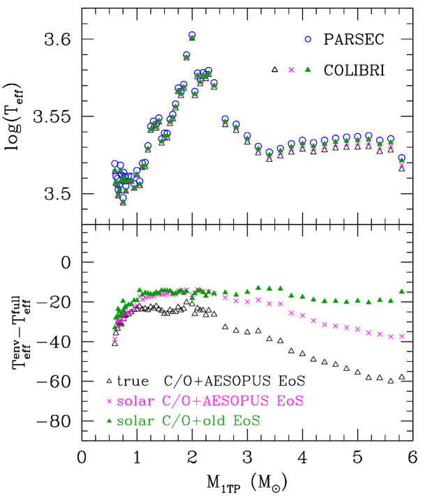
Figure 32: Accuracy tests on the effective temperature. Top panel: $T_{\rm eff}$ values as a function of the stellar mass at the $1^{\rm st}$ thermal pulse for the set with ($Z_{\rm i}=0.01,\,Y_{i}=0.267$), as predicted by PARSEC full stellar models ($T_{\rm eff}^{\rm full}$) and by COLIBRI envelope-integration method ($T_{\rm eff}^{\rm env}$) for different assumptions of the abundance distribution and the EoS. Bottom panel: Differences $T_{\rm eff}^{\rm full}-T_{\rm eff}^{\rm env}$ in Kelvin degrees.

Considering that part of the differences is likely due to unavoidable numerical effects impossible to be disentangled, we have also investigated other possible physical causes that may explain some systematic trends. In particular we have considered the effects due to different descriptions of the EoS and the opacities in the PARSEC and COLIBRI codes.

In the bottom panel of Fig. 32 we zoom in the difference $T_{\rm eff}^{\rm env}-T_{\rm eff}^{\rm full}$ (in $K$ degrees), as a function of the stellar mass. The three sequences are obtained with three combinations of the EoS and low-$T$ opacities used in the COLIBRI code. The lowest sequence (black empty triangles), showing the largest deviations from PARSEC, corresponds to the $T_{\rm eff}^{\rm env}$ predictions with the optimal configuration of all input physics in COLIBRI. Specifically, envelope integrations have been carried out with both the EoS and the Rosseland mean opacities computed with ÆSOPUS on-the-fly according to the actual chemical mixture of all elements.

This implies that the molecular chemistry is accurately solved, exactly complying with the true surface C/O ratio that characterizes each stellar model at the onset of the TP-AGB phase. In fact, the surface C/O ratio may have decreased, compared to its initial value at the main sequence (${\rm C/O}<{\rm C/O}_{\rm initial}=({\rm C/O})_{\odot}\simeq 0.55$ for the scaled-solar case under consideration), as a consequence of the first dredge-up and, in stars with $M>4\,M_{\odot}$, because of the second dredge-up.

In contrast, in PARSEC the opacities are derived through interpolations on pre-computed opacity tables as a function of temperature, density, hydrogen abundance, and current metallicity $Z$, while keeping the distribution of metals fixed to the initial configuration, $X_{i}/Z=X_{i,\odot}/Z_{\odot}$. In particular this means that that no change in the C/O ratio is considered, i.e. ${\rm C/O}=({\rm C/O})_{\odot}$ is assumed in all opacity tables.

To test the effect produced on the effective temperatures by low-$T$ opacities with a fixed chemical partition, we have performed a second run of envelope integrations setting the metals partition in the ÆSOPUS chemistry routine frozen to the scaled-solar one ($X_{i}/Z=X_{i,\odot}/Z_{i,\odot}$), as in PARSEC. The differences $(T_{\rm eff}^{\rm env}-T_{\rm eff}^{\rm full})$ are now smaller, as one can see in Fig. 32 comparing the sequence of magenta crosses with that of black triangles. In this case the temperature differences are mostly comprised within $25$ K, and in all cases lower than $40$ K. The fact the assumed solar C/O ratio is higher than the actual values at the $1^{\rm st}$ TP, implies that a smaller excess of oxygen atoms, (O-C), is available to form the H₂O molecule, the most efficient opacity source at the atmospheric temperatures under consideration. The effect seems to be somewhat larger at increasing stellar mass.

Finally, we have explored possible additional EoS effects. At this stage we cannot obtain a quantitative comparison with respect to PARSEC, in which the EoS is solved with the FreeEOS code, since these latter is not implemented in our COLIBRI code. Anyway, to obtain an order-of-magnitude estimate, we have carried out a third run of envelope integrations, switching the EoS option from the ÆSOPUS routine to an older and simpler EoS description based on Kippenhahn, Thomas & Weigert (1965). We see that now the deviations $T_{\rm eff}^{\rm env}-T_{\rm eff}^{\rm full}$ reduce further, keeping of the order of $\approx 20\,K$ or lower. Therefore we may conclude that the EoS treatment may also explain part of the differences $T_{\rm eff}^{\rm env}-T_{\rm eff}^{\rm full}$, by an amount that is comparable to that driven by the opacities.

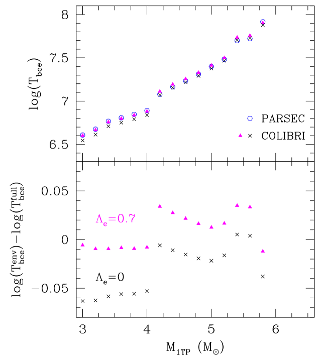
Figure 33: Accuracy tests on the temperature at the bottom of the convective envelope. Top panel: $T_{\rm bce}$ values a as a function of the stellar mass at the $1^{\rm st}$ thermal pulse for the set with ($Z_{\rm i}=0.01,\,Y_{i}=0.267$), as predicted by PARSEC full stellar models ($T_{\rm eff}^{\rm bce}$) and by COLIBRI envelope-integration method ($T_{\rm bce}^{\rm env}$) without and with convective overshooting beyond the formal Schwarzschild border. Bottom panel: Logarithmic difference $\log(T_{\rm bce}^{\rm full})-\log(T_{\rm eff}^{\rm env})$.

B.2 Temperature at the base of the convective envelope

The quantity $T_{\rm bce}$ provides an additional performance test of our envelope-integration method, and it is particularly relevant for massive AGB models ($M>4\,M_{\odot}$) as it measures the efficiency of hot-bottom burning.

In full stellar models calculated with PARSEC convective overshoot is applied to the formal Schwarzschild border of the envelope, with an efficiency parameter $\Lambda_{\rm e}=0.05$ for $M<M01$ and $\Lambda_{\rm e}=0.7$ for $M>M02$. The transition masses, with approximate values $M01\approx 1.0-1.5\,M_{\odot}$ and $M01\approx 1.5-2.0\,M_{\odot}$, are operatively defined in Bressan et al. (2012) and depend on chemical composition.

We apply the same scheme to our envelope integrations and then compare the predictions for $T_{\rm bce}$ as a function of stellar mass and metallicity. Results are shown in Fig. 33. We have verified that variations in the EoS and opacities, as those discussed in Sect. B.1, produce almost negligible changes in $T_{\rm bce}$ for the models under considerations, so that we do not show the corresponding results.

The effect of convective overshoot on $T_{\rm bce}$ is illustrated in Fig. 33 for the set with initial chemical composition $Z_{\rm i}=0.01,Y_{i}=0.267$. As a general rule models with $\Lambda_{\rm e}>0$ tend to have higher $T_{\rm bce}$ since the base of the convective envelope penetrates more deeply inward. For masses $M<M01$ the differences in $T_{\rm bce}^{\rm env}$ remain small among models with or without overshoot, with $[\log T_{\rm bce}^{\rm env}(\Lambda_{\rm e}=0.05)-\log T_{\rm bce}^{\rm env}(\Lambda_{\rm e}=0)]\la 0.006$, reflecting the little overshoot efficiency adopted in since this mass range. In all cases $\log(T_{\rm bce}^{\rm full})-\log(T_{\rm bce}^{\rm env})$ keep positive, i.e. the envelope-integration method yields somewhat higher temperatures than full stellar models.

Larger differences in $T_{\rm bce}^{\rm env}$ arise instead for masses $M>M02$, depending on whether we assume or not convective overshoot. We see that passing from $\Lambda_{\rm e}=0.7$ to $\Lambda_{\rm e}=0$ in our envelope integrations the differences $\log(T_{\rm bce}^{\rm full})-\log(T_{\rm bce}^{\rm env})$ tend to become negative, i.e. the envelope-integration method yields lower temperatures than full stellar models. A systematic decrease of $[\log T_{\rm bce}^{\rm env}(\Lambda_{\rm e}=0.7)-\log T_{\rm bce}^{\rm env}(\Lambda_{\rm e}=0)]\simeq 0.03-0.05$ is predicted for these models.

In general the deviations from the full stellar models are larger than those for the effective temperatures, with $|\log(T_{\rm bce}^{\rm full})-\log(T_{\rm eff}^{\rm env})|$ reaching up to a few hundredths of a dex. Part of the reason likely resides in the operative definition of the convective border and the adopted mass meshing across the envelope. In our COLIBRI code the classical Schwarzschild border is determined by the equality between the radiative and adiabatic temperature gradients, $\nabla_{\rm rad}=\nabla_{\rm ad}$, and all physical quantities are derived from interpolation between the last convective mesh and the first radiative one during the inward envelope integration. In PARSEC the Schwarzschild border is assumed to coincide with the last convective mesh, without interpolation in temperature gradients.

Limiting to the COLIBRI models with $\Lambda_{\rm e}>0$, we note that larger deviations from $T^{\rm full}_{\rm bce}$ are found at larger stellar masses ($M>4\,M_{\odot}$) where HBB starts to be operative. Part of these differences are likely related to the arrangement of the mesh points across the envelope; in fact the base of the convective envelope locates inside an extremely thin (in mass) region characterised by very steep gradients of all thermodynamic quantities ($T,P,\rho$, etc.), As a consequence, even small differences in mass resolution in this region may produce somewhat appreciable differences in the thermodynamic profile of the innermost layers of envelope.

We conclude that our envelope-integration method yields a description of the deepest envelope layers which is in satisfactory agreement with full stellar models, but unavoidable differences exist mainly due numerical and technical details. The size of such deviations are in any case lower than the current differences between various sets of AGB models, the latter reflecting the uncertainties of a still ill-defined theory of convection in stars.

References

- Angulo (1999) Angulo C., 1999, AIPC, 495, 365
- Arnett & Truran (1969) Arnett W. D., Truran J. W., 1969, ApJ, 157, 339
- Badnell et al. (2005) Badnell N. R., Bautista M. A., Butler K., Delahaye F., Mendoza C., Palmeri P., Zeippen C. J., Seaton M. J., 2005, MNRAS, 360, 458
- Bedijn (1988) Bedijn, P. J. 1988, A&A, 205, 105
- Blöcker (1995) Blöcker T., 1995, A&A, 297, 727
- Blöcker & Schoenberner (1991) Blöcker T., Schönberner D., 1991, A&A, 244, L43
- Böhm-Vitense (1958) Böhm-Vitense E., 1958, ZA, 46, 108
- Boothroyd, Sackmann & Wasserburg (1995) Boothroyd A. I., Sackmann I.-J., Wasserburg G. J., 1995, ApJ, 442, L21
- Boothroyd & Sackmann (1992) Boothroyd A. I., Sackmann I.-J., 1992, ApJ, 393, L21
- Boothroyd & Sackmann (1988b) Boothroyd A. I., Sackmann I.-J., 1988b, ApJ, 328, 671
- Boothroyd & Sackmann (1988a) Boothroyd A. I., Sackmann I.-J., 1988a, ApJ, 328, 641
- Blöcker & Schönberner (1991) Blöcker, T. & Schönberner, D. 1991, A&A, 244, L43
- Böhm-Vitense (1958) Böhm-Vitense E., 1958, ZA, 46, 108
- Bressan et al. (2012) Bressan A., Marigo P., Girardi L., Salasnich B., Dal Cero C., Rubele S., Nanni A., 2012, MNRAS, 427, 127
- Buchmann (1996) Buchmann L., 1996, ApJ, 468, L127
- Busso, Gallino & Wasserburg (1999) Busso M., Gallino R., Wasserburg G. J., 1999, ARA&A, 37, 239
- Caffau et al. (2011) Caffau E., Ludwig H.-G., Steffen M., Freytag B., Bonifacio P., 2011, SoPh, 268, 255
- Cameron & Fowler (1971) Cameron A. G. W., Fowler W. A., 1971, ApJ, 164, 111
- Carretta et al. (2009) Carretta E., et al., 2009, A&A, 505, 117
- Caughlan & Fowler (1988) Caughlan G. R., Fowler W. A., 1988, ADNDT, 40, 283
- Chafa et al. (2007) Chafa A., et al., 2007, PhRvC, 75, 035810
- Cole et al. (2005) Cole A. A., Tolstoy E., Gallagher J. S., III, Smecker-Hane T. A., 2005, AJ, 129, 1465
- Conroy, Gunn & White (2009) Conroy C., Gunn J. E., White M., 2009, ApJ, 699, 486
- Cordier et al. (2007) Cordier D., Pietrinferni A., Cassisi S., Salaris M., 2007, AJ, 133, 468
- Cox & Giuli (1968) Cox J. P., Giuli, R. T., 1968, in Principles of stellar structure - Vol.1: Physical principles, Gordon and Breach, Science Publishers, New York
- Cristallo et al. (2011) Cristallo S., et al., 2011, ApJS, 197, 17
- Cristallo et al. (2009) Cristallo S., Straniero O., Gallino R., Piersanti L., Domínguez I., Lederer M. T., 2009, ApJ, 696, 797
- Cristallo et al. (2007) Cristallo S., Straniero O., Lederer M. T., Aringer B., 2007, ApJ, 667, 489
- Cyburt et al. (2010) Cyburt R. H., et al., 2010, ApJS, 189, 240
- Dababneh et al. (2003) Dababneh S., Heil M., Käppeler F., Görres J., Wiescher M., Reifarth R., Leiste H., 2003, PhRvC, 68, 025801
- Denissenkov & Herwig (2003) Denissenkov P. A., Herwig F., 2003, ApJ, 590, L99