Asymmetric Ejecta Distribution in SN 1006

Abstract

We present the results from deep X-ray observations ($\sim 400$ ks in total) of SN 1006 by the X-ray astronomy satellite Suzaku. The thermal spectrum from the entire supernova remnant (SNR) exhibits prominent emission lines of O, Ne, Mg, Si, S, Ar, Ca, and Fe. The observed abundance pattern in the ejecta components is in good agreement with that predicted by a standard model of Type Ia supernovae (SNe). The spatially resolved analysis reveals that the distribution of the O-burning and incomplete Si-burning products (Si, S, and Ar) is asymmetric, while that of the C-burning products (O, Ne, and Mg) is relatively uniform in the SNR interior. The peak position of the former is clearly shifted by $5\arcmin$ ($\sim$3.2 pc at a distance of 2.2 kpc) to the southeast from the SNR’s geometric center. Using the SNR age of $\sim$1000 yr, we constrain the velocity asymmetry (in projection) of ejecta to be $\sim$3100 km s^-1. The abundance of Fe is also significantly higher in the southeast region than in the northwest region. Given that the non-uniformity is observed only among the heavier elements (Si through Fe), we argue that SN 1006 originates from an asymmetric explosion, as is expected from recent multi-dimensional simulations of Type Ia SNe, although we cannot eliminate the possibility that an inhomogeneous ambient medium induced the apparent non-uniformity. Possible evidence for the Cr K-shell line and line broadening in the Fe K-shell emission is also found.

1. Introduction

Despite many efforts in the last decades, the explosion mechanism of Type Ia supernovae (SNe) is still unclear. It is widely known that Type Ia SNe show significant diversity in the optical spectra and the light curves (e.g., Phillips et al., 1999; Benetti et al., 2005). Theoretically, the diversity has been interpreted as a consequence of spherically asymmetric explosions (e.g., Kasen et al. 2009; also see Mazzali et al. 2007). Maeda et al. (2010) systematically studied Type Ia SNe and attributed the observed spectral diversity to random viewing angles in almost identically symmetric explosions. Besides them, multi-dimensional simulations have suggested that thermonuclear ignition in Type Ia progenitors is offset from the center (e.g., Woosley et al., 2004; Kuhlen et al., 2006; Röpke et al., 2007), which may result in a non-uniform distribution of the nucleosynthesis products.

Young supernova remnants (SNRs) in our Galaxy are ideal sites to investigate the abundance and distribution of SN ejecta in detail, because they are spatially well resolved, unlike extragalactic SNe. SN 1006, one of the prototypical Type Ia SNRs, is particularly appealing for such investigation owing to its proximity (2.2 kpc: Winkler et al., 2003) and moderate angular size ($30\arcmin$ in diameter). It is located at a high Galactic latitude ($b=14.6$) and hence has small foreground extinction. SN 1006 is therefore a suitable object to investigate the spatial information of low-$Z$ elements, such as O, Ne, and Mg, for which K-shell emissions are observed in soft X-rays. Its low and uniform ambient density (Dubner et al., 2002) also enables us to study its nearly pure distribution of ejecta, with no significant modification owing to the swept-up interstellar medium (ISM). Nonetheless, our knowledge of ejecta has been limited because previous studies on SN 1006 have been mostly on the northeast (NE) and southwest (SW) rims, where the cosmic-ray acceleration (non-thermal X-ray) is dominant (e.g., Koyama et al., 1995; Bamba et al., 2003; Cassam-Chenaï et al., 2008).

Although Type Ia SNe yield a large amount of Fe (e.g., Iwamoto et al., 1999), detection of any signature of Fe ejecta from SN 1006 is hampered. One reason is that the thermal X-ray radiation from ejecta is faint compared to the bright non-thermal emissions, mainly from the cosmic-ray-accelerating rims. Furthermore, considerable fractions of ejecta may still not be shocked to emit X-rays. In fact, blue- and red-shifted absorption lines of Fe II were detected in the UV spectra of the background stars, suggesting that un-shocked Fe ejecta freely expands in the SNR’s interior (Wu et al., 1993; Hamilton et al., 1997; Winkler et al., 2005). However, the inferred amount of cool Fe ($<0.2M_{\odot}$) was much less than that of the theoretical prediction for a typical Type Ia SN ($\sim 0.7M_{\odot}$). Thus, a large amount of shocked Fe may exist in the SNR. Possible evidence for the shocked Fe ejecta (i.e., X-ray line emission) in SN 1006 was first reported from the BeppoSAX observation (Vink et al., 2000). Yamaguchi et al. (2008) found clearer evidence for the Fe K-shell line at $6.43(\pm 0.02)$ keV using Suzaku. The mean ionization age of Fe corresponding to this centroid energy was found to be much lower than those of the other lighter elements (e.g., Si, S), suggesting that the Fe-rich core was heated by the reverse shock more recently.

Yamaguchi et al. (2008) also revealed that the Fe K-shell lines are the brightest in the southeast (SE) quadrant, which may imply an asymmetric distribution of Fe-rich ejecta. However, the detailed spectroscopy was limited within the SE region, and spatial distributions of the other lighter elements were not well investigated.

In this paper, we report a comprehensive study on the shocked ejecta in SN 1006 using the deep exposure ($>400$ ks) data of Suzaku. Owing to the high sensitivity and good energy resolution, we are able to reveal detailed distribution of ejecta. Throughout this paper, the distance to SN 1006 is assumed to be 2.2 kpc (Winkler et al., 2003), and errors are quoted at a 90% confidence level unless otherwise noted.

Table 1Observation logs.

	Name	Obs. ID	Obs. Date	(R.A., Dec.) J2000	Exposure
Source	NE	100019020	2005-Sep-09	(225.9608, -41.7805)	22 ks
	SW1	100019030	2005-Sep-10	(225.5010, -42.0706)	31 ks
	SW2	100019050	2006-Jan-26	(225.4998, -42.0701)	31 ks
	SE	500016010	2006-Jan-30	(225.8686, -42.0508)	52 ks
	NW	500017010	2006-Jan-31	(225.6397, -41.7993)	53 ks
	Center	502046010	2008-Feb-25	(225.7268, -41.9424)	212 ks
Background	NE_BGD	100019010	2005-Sep-04	(226.7036, -41.3998)	45 ks
	SW_BGD1	100019040	2005-Sep-11	(224.6550, -42.4005)	32 ks
	SW_BGD2	100019060	2006-Jan-26	(224.6468, -42.4025)	28 ks

2. Observations and Data Reduction

We performed several pointing observations of SN 1006 with the X-ray Imaging Spectrometer (XIS; Koyama et al., 2007) on board Suzaku (Mitsuda et al., 2007). The series of the observations covers almost the entire region of the SNR (Figure 1). The observations of the four quadrant regions were made during the performance verification (PV) phase by the Suzaku Science Working Group (SWG). To compensate for the relatively low sensitivity near the edge of each field of view (FoV) and to study more about the ejecta in the SNR interior, we performed a deeper observation aiming at the SNR’s center during the Announcement of Opportunity cycle 2 (AO2) phase. Detailed information about the observations made is summarized in Table 1. We used XIS1 (back-illuminated CCD; BI CCD), and XIS0, 2, and 3 (front-illuminated CCDs; FI CCDs) for the PV-phase data. However, for the AO2, XIS2 data were not available owing to possible damage by a micrometeorite on November 9, 2006. We used revision 2.4 of the cleaned event data and combined the $3\times 3$ and $5\times 5$ pixel events. The calibration database (CALDB) updated in September 2011 was used for data reprocessing. We performed data reduction with version 6.11 of the HEAsoft tools (version 18 of the Suzaku software).

Figure 1.— Vignetting-corrected XIS image of SN 1006 in the 0.4–5.0 keV band. The FoVs of XISs are shown with the solid squares. The cross mark indicates the geometric center of SN 1006. The dashed line regions are bright non-thermal rims with a background point source (QSO 1504-4152; Winkler & Long, 1997), which are excluded for the thermal spectrum analysis.

Figure 2.— Left: FI spectra of the thermal and non-thermal regions in SN 1006, where the NXB and CXB are subtracted. The spectrum of the BGD region is also shown. Right: The magnified spectrum of the thermal region in 5.0–10.0 keV.

3. Analysis and Results

We employed the xisrmfgen XIS response generator and the xissimarfgen ray-tracing-based ancillary response file generator to generate the redistribution matrix files and the ancillary response files, respectively (Ishisaki et al., 2007). For the following spectral analysis, we used the XSPEC software, version 12.7.0 (Arnaud, 1996). The data of the FI and BI CCDs were simultaneously analyzed, but only the FI spectra are shown throughout this paper for simplicity.

3.1. Galactic X-ray Background

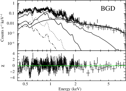
Figure 3.— Background spectrum fitted with several model components. The dashed-dotted and dotted lines show emissions from SB and MWH, respectively. The spectra of the local excess and the Lupus Loop are fitted with a power-law and two thermal components, respectively (the solid lines).

Table 2Best-fit parameters of the BGD spectrum.

Component	$N\rm_{H}$ ($\times 10^{20}$ cm-2)	$kT_{\rm e}$ (keV)	$\Gamma$	flux ($\times 10^{-12}$ ergs cm-2 s-1)
SB (CIE)	$\cdots$	0.1 (fixed)	$\cdots$	$<0.55$
MWH (CIE)	5.6 (fixed)	0.1 (fixed)	$\cdots$	$2.43\pm 0.21$
Local Excess (Power-law)	1.0 (fixed)	$\cdots$	$1.9\pm 0.1$	$1.68\pm 0.14$
The Lupus Loop1 (CIE)	1.0 (fixed)	$0.22\pm 0.01$	$\cdots$	$3.22\pm 0.14$
The Lupus Loop2 (CIE)	1.0 (fixed)	$0.98\pm 0.01$	$\cdots$	$1.28\pm 0.07$
$\chi^{2}$/dof				$439/355=1.24$

The combined XIS image of SN 1006 after subtraction of the non-X-ray background (NXB) (xisnxbgen; Tawa et al., 2008) is shown in Figure 1. First, we divided the entire SNR into “non-thermal” and “thermal” regions and extracted spectra using all five of the pointing observations. The non-thermal regions consist of the NE and SW rims confined with the dotted lines in Figure 1, while the thermal region is the whole remaining area. We subtracted the cosmic X-ray background (CXB) from each spectrum by applying a power-law model with a photon index of 1.4 (Kushino et al., 2002).

The left panel of Figure 2 shows the NXB/CXB-subtracted spectra of the non-thermal and thermal regions. K-shell lines of O, Ne, Mg, Si, S, Ar, Ca, and Fe were clearly detected in the thermal spectrum. To see more detail around the Fe K-shell line, we show the 5–10 keV band spectrum in the right panel of Figure 2. Besides the Fe K-shell line, we see a line-like structure at $\sim$5.4 keV.

We obtained the Galactic X-ray background (BGD) data from three near-sky pointing observations of SN 1006 (BGD: Table 1). The combined BGD spectrum after the subtraction of the NXB and CXB is shown in Figure 2. Although the BGD regions (and SN 1006) are located far off from the Galactic plane, we found clearly noticeable excess X-rays. The excess X-rays were previously found with the Tenma satellite (Koyama et al., 1987). Although their origin (thermal or non-thermal) was unclear, it was well described by a power-law model with a photon index of $2.1\pm 0.1$. Ozaki et al. (1994) confirmed the excess X-rays with the Ginga satellite and represented the spectrum using a thermal bremsstrahlung model with a temperature of 7 keV. Soft X-rays from an evolved SNR, the Lupus Loop (Winkler et al., 1979), are widely spread over the full area of SN 1006, and hence would contaminate the soft X-ray band. In addition, the possible contribution of the soft background (SB), which was often observed from off-plane sky regions such as the North Polar Spur (Miller et al., 2008) and the Milky Way halo (MWH), should not be ignored.

Because the observation dates of the SNR Center (AO2) and the BGD regions (PV phase) are largely separated, the difference in the energy resolution and event-detection efficiency among these observations cannot be ignored. We therefore made a model of the BGD spectrum, and added it to the source spectrum for the following fitting procedures, instead of applying direct BGD subtraction.

As we noted, the BGD model should be composed of a power-law plus several thermal components with different electron temperatures. We fit the BGD spectrum with a model of these components. The best-fit results are shown in Figure 3 and Table 2. The photon index of the local excess was obtained to be $1.9\pm 0.1$, consistent with the result of Koyama et al. (1987). We also found that the Lupus Loop has two temperature spectra with $\sim$0.22 keV and $\sim$0.98 keV.

We then renormalized the flux of the BGD model by the effective area and added it to the source spectrum as the background components. We fixed all the BGD parameters determined in this way. To confirm the reliability of the background model, we fitted the spectrum of the non-thermal rims (NE and SW) with a power-law plus the BGD model, and obtained the best-fit photon index of $\sim$2.8. This value is consistent with a typical index of the synchrotron radiation in the X-ray band from the non-thermal rims of SN 1006 (e.g., Koyama et al., 1995).

3.2. Spectrum of the Entire Thermal Region

Yamaguchi et al. (2008) found that the Si and S-K$\alpha$ lines in the spectrum of the SE region are significantly broadened compared to those expected from a single non-equilibrium ionization (NEI) plasma model. This broadening was interpreted as a superposition of multiple ejecta components with different ionization timescales. We found similar line broadening in the entire thermal spectrum, and hence applied two NEI plasma components with variable abundances (VNEI, NEIvers2.0$+$; Borkowski et al., 2001) to represent high- and low-ionization ejecta of SN 1006 (hereafter Ejecta1 and Ejecta2, respectively). Free parameters were the electron temperature $kT_{\rm e}$, ionization timescale $n_{\rm e}t$, emission measure $EM=\int n_{\rm e}n_{\rm H}dV$, and column density $N{\rm{}_{H}}$ for interstellar absorption. Here $n_{\rm e}$, $n_{\rm H}$, $t$, and $V$ are the number densities of electrons and protons, elapsed time and the X-ray emitting volume, respectively.

Table 3Best fit parameters (see Figure 4)

Component	Parameter		Value
Absorption	$N\rm_{H}$ ($\times 10^{20}$ cm-2)		$6.80\pm 0.07$
Ejecta1 (VNEI)	$kT_{\rm e}$ (keV)		$0.48\pm 0.01$
	Abundance ($10^{4}$ solar)	C	0 (fixed)
		N	0 (fixed)
		O	1.0 (fixed)
		Ne	$0.53\pm 0.02$
		Mg	$3.71\pm 0.07$
		Si	$13.7\pm 0.3$
		S	$30\pm 1$
		Ar	$27\pm 1$
		Ca	$160\pm 8$
		Fe	$0.56\pm 0.01$
		Ni	(=Fe)
	$n_{\rm e}t$ (cm-3 s)		$4.39\pm 0.05\times 10^{10}$
	flux (ergs cm-2 s-1)		$7.85\pm 0.01\times 10^{-11}$
Ejecta2 (VNEI)	$kT_{\rm e}$ (keV)		$1.73\pm 0.03$
	Abundance ($10^{4}$ solar)	C	0 (fixed)
		N	0 (fixed)
		O	1.0 (fixed)
		Ne	$0.53\pm 0.01$
		Mg	$2.3\pm 0.1$
		Si	$23.9\pm 0.4$
		S	$25.2\pm 0.8$
		Ar	$26\pm 3$
		Ca	(=Fe)
		Fe	$43\pm 3$
		Ni	(=Fe)
	$n_{\rm e}t$ (cm-3 s)		$1.40\pm 0.01\times 10^{9}$
	flux (ergs cm-2 s-1)		$8.66\pm 0.01\times 10^{-11}$
ISM (NEI)	$kT_{\rm e}$ (keV)		$0.4\pm 0.1$
	$n_{\rm e}t$ (cm-3 s)		$5.1^{+0.8}_{-0.6}\times 10^{9}$
	flux (ergs cm-2 s-1)		$4.60\pm 0.01\times 10^{-11}$
Power-law	$\Gamma$		$3.11\pm 0.02$
	flux (photons cm-2 s-1)		$3.64\pm 0.03\times 10^{-2}$
Emission Line	Center Energy (keV)	Normalization (photons cm-2 s-1)	1-$\sigma$ Width (eV)
Fe-L + O VII-K	$0.73\pm 0.01$	$3.92\pm 0.08\times 10^{-3}$	0 (fixed)
Ca-K	3.69 (fixed)	$1.8\pm 0.4\times 10^{-5}$	0 (fixed)
Cr-K	$5.42^{+0.20}_{-0.11}$	$3\pm 2\times 10^{-6}$	0 (fixed)
Fe-K	$6.45\pm 0.02$	$2.6\pm 0.4\times 10^{-5}$	$101^{+33}_{-27}$
$\chi^{2}$/dof			$1225/838=1.46$

Because Type Ia SN ejecta should have a pure-metal composition with little contribution from H and He, we fixed the abundance of oxygen (Anders & Grevesse, 1989) to be a sufficiently high value ($1\times 10^{4}$ solar), so that the bremsstrahlung from these elements is negligible compared to those originating from the heavy element ions. Abundances of C and N were fixed at 0, while those of Ne, Mg, Si, S, Ar, and Fe were allowed to vary freely and that of Ni was linked to Fe. For Ejecta2, the Ca abundance was also linked to Fe, but for Ejecta1, Ca abundance was a free parameter because L-shell lines of Ca may contribute to the spectrum in the soft X-ray band ($<0.5$ keV; see Ejecta-1 component in Figure 4).

Because the ionization time scale for Fe is very low (Yamaguchi et al., 2008), Ca would also emit K-shell lines from low ionization states (Ejecta2). However, the current NEI model does not include such emission lines. We therefore added a Gaussian line at 3.69 keV to represent the low-ionization Ca K-shell line in Ejecta2. We also added an NEI model with the solar abundances and a power-law to represent the swept-up ISM and the non-thermal emissions, respectively. The energy band around the neutral Si K edge (1.7–1.8 keV) was ignored because the current response function was not accurate in this limited energy band. We also eliminated the 0.5–0.63 keV band because the calibration of the contamination on the optical blocking filter was problematic.

In this initial fit, we found a “shoulder”-shaped residual at around 0.7–0.8 keV. This feature was already noticed by Yamaguchi et al. (2008) and interpreted to be a higher transition series of the O VII K-shell lines (i.e., K$\delta$ and K$\epsilon$, which are not incorporated in public NEI models). Because our NEI model also lacks the O VII K-shell lines higher than K$\delta$, we added two Gaussian lines at 723 eV and 730 eV to represent K$\epsilon$ and K$\zeta$, respectively. The intensity ratio of K$\zeta$/K$\epsilon$ was assumed to be 0.5 (Yamaguchi et al., 2008) or 0.75 (Broersen et al., 2012). Although this fit was significantly improved ($\chi^{2}$/dof was reduced from 1300/839 to 1225/838) in both cases, we need an unreasonably high intensity ratio of K$\epsilon$ and K$\zeta$ compared to that of lower-excitation level (e.g., K$\epsilon$/K$\delta\sim 3.4$). This may require an additional line for the excess around 0.7 keV.

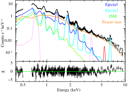
Figure 4.— FI spectrum of the thermal region fitted with the four-component model plus additional Gaussian lines: Ejecta1 (blue), Ejecta2 (light blue), ISM (light green), a non-thermal power-law (orange), and the magenta and red Gaussian lines for missing lines (see text).

Usually, this energy band is dominated by the Fe XVII L-shell emission of the 3s$\rightarrow$2p transition with flux comparable to the emission of the 3d$\rightarrow$2p transition at $\sim 0.8$ keV (Foster et al., 2012). However, in an extremely low-ionized plasma, L-shell emissions from even lower-charged Fe are also expected to occur following inner L-shell ionization. Although they can contribute to the spectrum around 0.7 keV, the current NEI code does not include any emission from these ions. In fact, our initial best-fit $kT_{\rm e}\sim 1.7$ keV and $n_{\rm e}t\sim 1\times 10^{9}$ cm^-3 s (for Ejecta2) predicts that the most dominant charge state of Fe is less than Fe¹⁶⁺. Another young Type Ia SNR, E0509$-$67.5, which also has an extremely low-ionization timescale of Fe ($n_{\rm e}t<2\times 10^{9}$ cm^-3; Kosenko et al., 2008), shows a similar excess around 0.7 keV (Warren & Hughes, 2004). The weakness of the O VII and O VIII emissions in SNR E0509$-$67.5 (Warren & Hughes, 2004; Badenes et al., 2008) leads the excess to be mainly owing to the Fe L-shell emission. Because the O VII K$\alpha$ line is strong in SN 1006 (Figure 4 and Table 3), both the higher K-shell transitions of O VII and Fe L-shell emissions should be considered in the excess around 0.7 keV. For simplicity, we combined all the relevant lines (O VII-K$\epsilon$, K$\zeta$, and Fe L 3d$\rightarrow$2p transitions) to a single Gaussian line at around 0.7 keV. As we noted in the previous subsection, we found a line-like structure at $\sim 5.4$ keV. We therefore added a Gaussian line in the final fitting. Then the center energy and flux were determined to be $5.42^{+0.20}_{-0.11}$ keV and $3{\pm 2}$ photons cm^-2 s^-1, respectively.

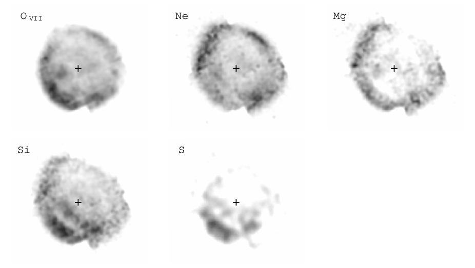
Figure 5.— Vignetting-corrected intensity maps of the K$\alpha$ lines from O, Mg, and Si. The geometric center of SN 1006 is indicated with the cross marks.

The best-fit results of this final model are given in Figure 4 and Table 3. The results are basically the same as those of Yamaguchi et al. (2008); the spectrum consists of a power-law, and plasmas of ISM and two ejecta components with different ionization timescales. The abundances of both ejecta components are also consistent with each other for Ne through Ar within a factor of $\sim$2, whereas the Fe abundance in Ejecta2 is more than one order of magnitude larger than that in Ejecta1.

In Figure 4, we see excess structures at both sides of the line at $\sim 6.4$ keV. This feature is likely owing to the broadening of the Fe K$\alpha$ line. We therefore fit the line with a Gaussian model and found the line energy and width to be $6.45{\pm 0.02}$ keV and $101^{+33}_{-27}$ eV, respectively (Table 3). Although Ejecta1 has an extremely large abundance of Ca (Table 3), this value should be considered cautiously because the Ca abundance is mainly determined by the L-shell lines for which uncertainty in the atomic data is large.

We found that the contribution of the ISM component is relatively lower than the result of SE (Figure 8 in Yamaguchi et al., 2008), but is consistent with the interpretation by Cassam-Chenaï et al. (2008). The O emission in the entire SNR predominantly originates from the shock heated ejecta rather than from the ISM.

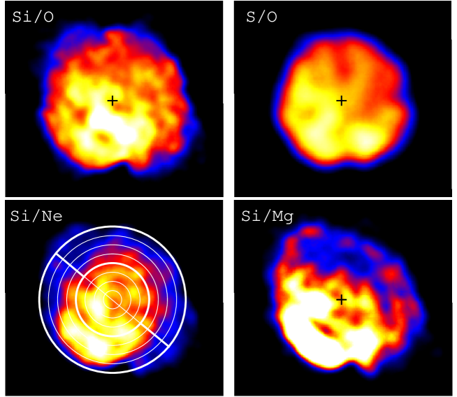
Figure 6.— Images of the line flux ratio of the K$\alpha$ lines from Si to O, S to O, Si to Ne, and Si to Mg. The geometric center of SN 1006 is shown with cross marks. The spectral extraction regions are shown with thin white lines. The width of each annulus is 2′. Thick white lines divide the remnant into three parts named as S (southeast), C (center), and N (northwest).

3.3. Spatially Resolved Analysis

Figure 5 shows the vignetting-corrected narrow band images of the K$\alpha$ lines from O, Ne, Mg, Si, and S, after subtraction of the underlying continuum levels estimated by the interpolation of the adjacent band fluxes. The images show rim-brightening morphology, particularly in the light elements such as O, Ne, and Mg. In the interior regions, O, Ne, and Mg are rather uniformly distributed. In contrast, the distributions of Si and S are more asymmetric in the inner region; the SE rim is much brighter than the other regions, and the “second shell” can be seen at the middle between the outermost shell and the SNR’s center. We also present the ratios of Si/O, S/O, Si/Ne, and Si/Mg in Figure 6. All the ratios show clear increases toward the SE rim, suggesting asymmetric ejecta distribution for the heavier elements (i.e., Si, S).

To investigate more quantitatively, we divided the entire SNR into three regions: a center circle of 8′-radius (C), and half-annuluses for the northwest (N) and southeast (S) (the thick white lines in Figure 6). The geometric center of the remnant was defined to be ($\alpha$, $\delta$)_J2000.0 = (225.7371, –41.9336). The spectra of these three regions are shown in Figure 7. We fitted the spectra with the same four-component model (and the same assumptions) applied for the entire thermal spectrum. The best-fit results are given in Table 4. We found that the heavier elements are indeed more abundant in the region S than in the region N.

We further divided the whole SNR into 16 regions: 8 annuli with widths of 2′, each divided into half-rings of the northwest (NW) and southeast (SE) areas (solid lines in Figure 6). Then we fitted each spectra with the same four-component model. Because the statistics of the Fe line were insufficient, we fixed its abundance to the best-fit value in Table 4. The best-fit $EM$s for each element in ejecta (Electa1+ Ejecta2) are given in Figure 8.

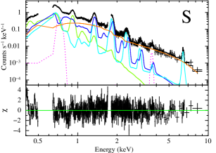
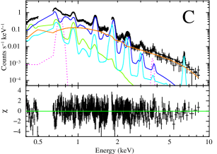
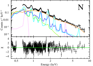
Figure 7.— FI spectrum of SN 1006 obtained from the regions S, C, and N. Each spectrum was fitted with the same four-component model as the whole region.

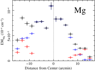
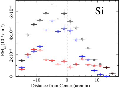
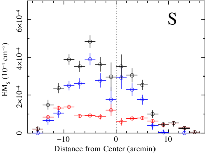
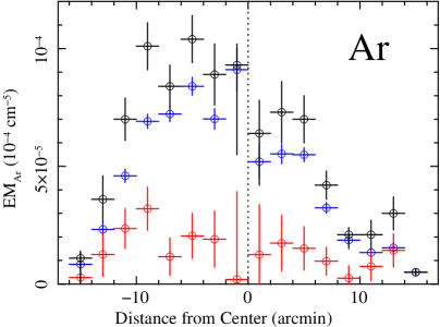
Figure 8.— Radial profiles of the emission measure ($EM$) for various elements (O, Mg, Si, S, Ar, and Fe) in ejecta. Red, blue, and black represent the results of Ejecta1, Ejecta2 (Table 3), and summation of them, respectively. Note that the vertical scales of the $EM$ of Mg and Ar ($EM_{\rm{Mg,Ar}}$) are 1/5 of those of O, Si, S, and Fe ($EM_{\rm{O,Si,S,Fe}}$). The horizontal axis shows the distance from the geometric center of SN 1006; the positive and negative values are the NW and SE sides, respectively.

Figure 9.— The K-shell line energy of Fe versus that of Cr in SN 1006. We also plotted previous results of W49B (Hwang et al., 2000), Tycho (Tamagawa et al., 2009), G 344.7-0.1 (Yamaguchi et al., 2012), and other remnants (Yang et al., 2013) with circles. Open squares at the lower-left and upper-right represent the values for the neutral and He-like states, respectively.

Table 4Best fit parameters (Figure 7).

Component	Parameter		Value
			Region S	Region C	Region N
Absorption	$N\rm_{H}$ ($\times 10^{20}$ cm-2)		$6.8\pm 0.1$	$6.8\pm 0.1$	$6.8\pm 0.2$
Ejecta1 (VNEI)	$kT_{\rm e}$ (keV)		$0.95\pm 0.01$	$0.95\pm 0.01$	$1.02^{+0.04}_{-0.03}$
	Abundance ($10^{4}$ solar)	C	0 (fixed)	0 (fixed)	0 (fixed)
		N	0 (fixed)	0 (fixed)	0 (fixed)
		O	1.0 (fixed)	1.0 (fixed)	1.0 (fixed)
		Ne	$0.45\pm 0.03$	$0.54\pm 0.02$	$0.45\pm 0.07$
		Mg	$3.0\pm 0.1$	$2.17\pm 0.05$	$2.4\pm 0.2$
		Si	$6.8\pm 0.2$	$6.7\pm 0.2$	$2.7\pm 0.4$
		S	$7.3\pm 0.8$	$8.8\pm 0.7$	$<2$
		Ar	$28\pm 2$	$14\pm 1$	$35\pm 5$
		Ca	$28\pm 2$	$34\pm 12$	$110\pm 50$
		Fe	$0.65\pm 0.02$	$0.40\pm 0.01$	$0.46\pm 0.05$
		Ni	(=Fe)	(=Fe)	(=Fe)
	$n_{\rm e}t$ (cm-3 s)		$2.66\pm 0.09\times 10^{10}$	$1.91\pm 0.05\times 10^{10}$	$1.8\pm 0.2\times 10^{10}$
	flux (ergs cm-2 s-1)		$1.02\pm 0.01\times 10^{-11}$	$1.73\pm 0.01\times 10^{-11}$	$0.32\pm 0.01\times 10^{-11}$
Ejecta2 (VNEI)	$kT_{\rm e}$ (keV)		$1.83^{+0.05}_{-0.04}$	$2.50\pm 0.09$	$2.74^{+0.18}_{-0.14}$
	Abundance ($10^{4}$ solar)	C	0 (fixed)	0 (fixed)	0 (fixed)
		N	0 (fixed)	0 (fixed)	0 (fixed)
		O	1.0 (fixed)	1.0 (fixed)	1.0 (fixed)
		Ne	$<0.02$	$0.41\pm 0.06$	$0.58\pm 0.03$
		Mg	$2.1\pm 0.2$	$3.3\pm 0.6$	$2.5\pm 0.2$
		Si	$24\pm 1$	$37\pm 2$	$12.9\pm 0.7$
		S	$30\pm 2$	$34\pm 3$	$10\pm 1$
		Ar	$14\pm 7$	$32\pm 10$	$<5$
		Ca	(=Fe)	(=Fe)	(=Fe)
		Fe	$20\pm 5$	$17\pm 5$	$3\pm 2$
		Ni	(=Fe)	(=Fe)	(=Fe)
	$n_{\rm e}t$ (cm-3 s)		$1.58\pm 0.02\times 10^{9}$	$1.31\pm 0.04\times 10^{9}$	$1.41\pm 0.02\times 10^{9}$
	flux (ergs cm-2 s-1)		$2.08\pm 0.04\times 10^{-11}$	$1.29\pm 0.01\times 10^{-11}$	$1.47\pm 0.01\times 10^{-11}$
ISM (NEI)	$kT_{\rm e}$ (keV)		0.4 (fixed)	0.4 (fixed)	0.4 (fixed)
	$n_{\rm e}t$ (cm-3 s)		$5.1\times 10^{9}$ (fixed)	$5.1\times 10^{9}$ (fixed)	$5.1\times 10^{9}$ (fixed)
	flux (ergs cm-2 s-1)		$2.22\pm 0.01\times 10^{-11}$	$1.76\pm 0.01\times 10^{-11}$	$0.91\pm 0.01\times 10^{-11}$
Power-law	$\Gamma$		$2.98\pm 0.03$	$3.16\pm 0.04$	$3.27\pm 0.03$
	flux (photons cm-2 s-1)		$0.68\pm 0.01\times 10^{-2}$	$0.64\pm 0.01\times 10^{-2}$	$0.63\pm 0.01\times 10^{-2}$
$\chi^{2}$/dof			$670/604=1.11$	$751/569=1.32$	$560/511=1.10$

4. Discussion

4.1. Elemental Abundances in Ejecta

In section 3.2, we successfully modeled the spectrum of the entire thermal region with the components applied previously by Yamaguchi et al. (2008). The emission lines of the heavy elements exhibit clear evidence for over-abundance relative to the solar values, indicating the SN ejecta origin. The difference in the ionization age between the two components suggests that Ejecta2 was heated more recently than Ejecta1. The suppressed relative abundance of Fe in Ejecta1 (Table 3) implies the absence of Fe in the outer ejecta layer, consistent with the previous claim by Yamaguchi et al. (2008).

We find a possible line feature at $\sim 5.4$ keV. This centroid energy suggests its origin to be a Cr K$\alpha$ emission. To examine this possibility, we plot in Figure 9 the Cr K$\alpha$ and Fe K$\alpha$ centroids observed in other SNRs (e.g., Yang et al., 2013) and compare with our results. We find that the values from SN 1006 are reasonably close to the previous Cr K$\alpha$–Fe K$\alpha$ centroid correlations, supporting our claim of the first detection of Cr from this remnant.

Because atomic data for Cr are not available in the current NEI model, we estimate the emissivity $\varepsilon_{\rm{Cr}}$ following the method of the ASCA measurement for W49B (Hwang et al., 2000). Using the best-fit temperature and the ionization timescale for Ejecta2 component, we calculate emissivities for Si, S, Ar, and Fe. The results are given in Figure 10. Interpolating these values to that of Cr, we estimated the Cr/Fe abundance ratio $Z_{\rm{Cr}}/Z_{\rm{Fe}}$ to be $2.5\pm 1.9$ solar. Here we assumed that Cr is mainly contained in Ejecta2, as is the case for Fe.

As we noted, the NEI model we used also lacks emission data for Ca in the low-ionization state (Ejecta2). Therefore, we estimated $Z_{\rm{Ca}}/Z_{\rm{Fe}}$ with the same method to be $0.8\pm 0.2$ in Ejecta2. This result is consistent with our initial assumption that the abundance of Ca is nearly equal to Fe in Ejecta2.

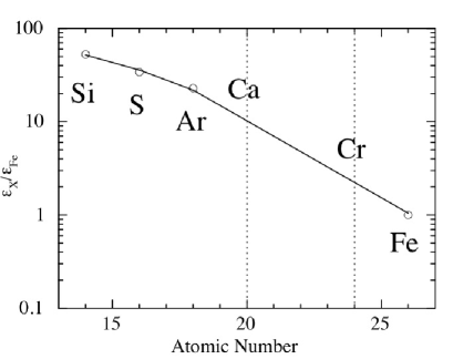
Figure 10.— Emissivity of heavy elements relative to that of Fe. These values were calculated from the NEI model of the best-fit Ejecta2 temperature and ionization parameter. The line is a spline fit to them.

We compare the abundances of Ejecta2 (relative to O) with the nucleosynthesis yields predicted by several theoretical models (Figure 11). We employ the Type Ia deflagration or delayed-detonation models (Iwamoto et al., 1999) and the core-collapse SN models with various progenitor masses (15$M_{\odot}$, 20$M_{\odot}$, 30$M_{\odot}$, and 40$M_{\odot}$; Woosley & Weaver, 1995). The observed abundance pattern is confirmed to be broadly consistent with the standard Type Ia models. The abundance ratios of Si/O, S/O, Ar/O, are Ca/O are enhanced compared to those predicted by the W7 deflagration model, and slightly closer to the yields of the delayed-detonation explosion (CDD1).

Figure 11.— Metal abundances of Ejecta2 relative to O as a function of atomic number (the solid line and X marks). The dashed lines and circles represent the Delayed Detonation, i.e., CDD1 (one of the DDT models) and classical deflagration model, W7 (Iwamoto et al., 1999). The dotted lines and triangles represent core-collapse models with main sequence masses of 15$M_{\odot}$, 20$M_{\odot}$, 30$M_{\odot}$, and 40$M_{\odot}$ (Woosley & Weaver, 1995).

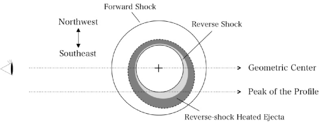
Figure 12.— Schematic diagram of the ejecta structure of SN 1006. The gray area represents ejecta already heated by the reverse shock. The light gray and dark gray regions correspond to the Fe-rich core and the Si-rich layer, respectively. The heavy elements are displaced to the far-side and the SE (see text).

4.2. Three-dimensional Geometry of SN 1006

The spherical outer shell with rim-brightening in O, Ne, and Mg (Figure 5) would be mainly owing to the ISM components, because ejecta distributions in Figure 8 show no enhancement in these regions. On the other hand, the interior is likely to be dominated by ejecta (e.g., Figure 8). Then ejecta distributions are broadly separated into two patterns: the uniform interior for the lighter elements (O, Ne, and Mg) and more asymmetric distributions of the heavier elements (Si and S) with peak positions offset by $5\arcmin$ ($\sim$3.2 pc). The off-center distribution of the heavier elements is also confirmed in Figure 6. Notably, these two groups (O-Ne-Mg and Si-S) are synthesized in different nuclear burning processes in Type Ia SNe explosions: C-burning for O-Ne-Mg compared to O-burning and incomplete Si-burning for Si-S. We thus presume that the latter products distribute more asymmetrically than the former products.

The asymmetry of ejecta should be formed either at the time of the SN explosion or in the process of the following interaction with the ISM. If the ambient density in the SE is higher than in the other regions, a reverse shock might heat up ejecta earlier, which may explain the relative enhancement of the $EM$ in the SE. To estimate the ambient densities in the SE and NW rims, we analyzed spectra from an annulus at the outer edges of the SE and NW. We fitted the spectra and found the best-fit normalizations ($EM$: emission measure) of the ISM components to be $2.46\pm 0.29\times 10^{-4}$ cm^-5 and $1.93\pm 0.22\times 10^{-4}$ cm^-5 for the SE and NW, respectively. Given that SN 1006 is a sphere with a radius of 10.2 pc, the volume of the annulus is estimated to be 35 pc³. Then, the ISM densities are $n_{\rm H}=0.11\pm 0.01$ cm^-3 and $0.09\pm 0.01$ cm^-3. The ambient densities ($n_{\rm H}/4)$ are thus $\sim 0.03$ cm^-3 and $\sim 0.02$ cm^-3, for SE and NW, respectively. Previous observations (e.g., Heng et al., 2007) indicate that the ambient density in the NW is 0.15–0.3 cm^-3, significantly higher than our result. Because the best-fit normalization ($EM$) was coupled with that of $n_{\rm e}t$ and anti-correlated to $kT_{\rm e}$, a higher value of $n_{\rm H}$/4 (up to $\sim 0.1$ cm^-3) is statistically acceptable in the NW. The annulus we used for the spectrum is broader than the outermost edge of the recent shock encounter. On the other hand, the forward shock in the NW has only interacted with the denser region fairly recently (Katsuda et al., 2013), which may explain the discrepancy between our result and the previous studies.

Accordingly, within possible statistical and systematic uncertainties, we can conclude that the ambient density in the SE is lower than 0.1 cm^-3 and does not particularly exceed those in the other rims. Furthermore, if an inhomogeneous ambient density has affected the large-scale variation of ejecta, the lighter elements (O, Ne, and Mg) should similarly distribute asymmetrically. As shown in Figure 6, the actual distributions clearly refute this hypothesis. Thus, it is more plausible that ejecta asymmetry was caused by an asymmetric SN explosion.

We found the “second shell” in Si and S at the middle between the outermost shell and the SNR’s center ($\sim 6\arcmin$ from the Center). The “second shell” is most likely from ejecta, because we see a peak of Si and S at this position in ejecta abundance (Figure 5). Because the foreground absorption is negligible in energies above $\sim 1.5$ keV, this second-shell structure is not owing to the absorption effect, but it likely originates from the ejecta rim, reminiscent of similar double-shell morphology in G299.2-2.9 (Park et al., 2007) (although this remnant is dominated by swept-up ISM, unlike SN 1006).

We also found that the $EM$ of Fe increases from NW to SE, as Yamaguchi et al. (2008) found that the Fe-rich core spreads out to SE. These results indicate that ejecta, particularly heavier elements in more inner regions, expand preferentially toward the SE. Based on the broad UV absorption lines of Si and Fe of several background objects, Hamilton et al. (1997) estimated that the diameter toward the far side of SN 1006 is roughly 20% larger than the rest of the remnant (see Figure 7 of Hamilton et al., 1997). Winkler et al. (2005) also confirmed the ejecta structure of Si and Fe by a similar analysis that the shell of SN 1006 is almost spherical (see Figure 8 of Winkler et al., 2005). We thus propose that ejecta expanded not only transverse to but also along the line of sight; ejecta were displaced toward the SE and far side of the center (Figure 12). If the reverse shock heated up a part of ejecta components, then the centrally peaked profile is easily understood (Figure 12). In addition, if the reverse shock recently reached to the surface of the Fe-rich core (light gray region in Figure 12), the $EM$ is higher at the shifted direction (lower right in Figure 12).

Including the “second shell”, the peak positions of the heavy elements (Si, S, and Ar) are $\sim 5\arcmin=3.2$ pc away from the geometric center toward the SE (Figure 8). Assuming a distance of 2.2 kpc and the SNR age of 1000 yr, we estimate that the velocity difference (owing to an asymmetric explosion) between the SE and NW direction is $\sim 3100$ km s^-1 in projection. We found that Fe K$\alpha$ is broadened by $101^{+33}_{-27}$ eV (1-$\sigma$), for the first time from SN 1006. If this width is owing to the Doppler broadening of ejecta, as is the case of Tycho (Hayato et al., 2010), the expansion velocity in the line of sight should be $\sim 3000$ km s^-1. This value is consistent with that of Katsuda et al. (2013), in which they measured the proper motion of the NW rim in X-ray.

5. Summary

This paper focused on the thermal spectrum of SN 1006 based on the deep observation ($\sim 400$ ks in total) with Suzaku XIS. The results are summarized as follows:

1. The X-ray spectra are well represented by a model with three NEI thermal plasmas (ejecta with different ionization parameters and ISM) plus one power-law component (non-thermal emission).

2. Ejecta abundance ratios of Ne, Mg, Si, S, Ar, Ca, Cr, and Fe relative to O are all in good agreement with yields predicted by the standard Type Ia theories: the classical carbon-deflagration model and the deflagration to detonation transition mechanism.

3. The distribution of the centroids of Si, S, and Ar are significantly shifted from the SNR’s geometric center by $\sim 3.2$ pc toward the SE, which we argue is likely to be associated with an asymmetric explosion of the progenitor. The velocity (in projection) difference of ejecta is $\sim$3100 km s^-1 at the distance of 2.2 kpc. The morphology of O, Ne, and Mg in the interior are more symmetric.

4. We found possible evidence for the Cr-K shell line and line broadening in the Fe-K shell emission.

References

- Anders & Grevesse (1989) Anders, E., & Grevesse, N. 1989, Geochim. Cosmochim. Acta, 53, 197
- Arnaud (1996) Arnaud, K. A. 1996, in Astronomical Society of the Pacific Conference Series, Vol. 101, Astronomical Data Analysis Software and Systems V, ed. G. H. Jacoby & J. Barnes, 17
- Badenes et al. (2006) Badenes, C., Borkowski, K. J., Hughes, J. P., Hwang, U., & Bravo, E. 2006, ApJ, 645, 1373
- Badenes et al. (2008) Badenes, C., Hughes, J. P., Cassam-Chenaï, G., & Bravo, E. 2008, ApJ, 680, 1149
- Bamba et al. (2003) Bamba, A., Yamazaki, R., Ueno, M., & Koyama, K. 2003, ApJ, 589, 827
- Benetti et al. (2005) Benetti, S., Cappellaro, E., Mazzali, P. A., et al. 2005, ApJ, 623, 1011
- Borkowski et al. (2001) Borkowski, K. J., Lyerly, W. J., & Reynolds, S. P. 2001, ApJ, 548, 820
- Broersen et al. (2012) Broersen, S., Vink, J., Miceli, M., et al. 2012, ArXiv e-prints
- Cassam-Chenaï et al. (2008) Cassam-Chenaï, G., Hughes, J. P., Reynoso, E. M., Badenes, C., & Moffett, D. 2008, ApJ, 680, 1180
- Dubner et al. (2002) Dubner, G. M., Giacani, E. B., Goss, W. M., Green, A. J., & Nyman, L.-Å. 2002, A&A, 387, 1047
- Foster et al. (2012) Foster, A. R., Ji, L., Smith, R. K., & Brickhouse, N. S. 2012, ApJ, 756, 128
- Hamilton et al. (1997) Hamilton, A. J. S., Fesen, R. A., Wu, C.-C., Crenshaw, D. M., & Sarazin, C. L. 1997, ApJ, 481, 838
- Hayato et al. (2010) Hayato, A., Yamaguchi, H., Tamagawa, T., et al. 2010, ApJ, 725, 894
- Heng et al. (2007) Heng, K., van Adelsberg, M., McCray, R., & Raymond, J. C. 2007, ApJ, 668, 275
- Hwang et al. (2000) Hwang, U., Petre, R., & Hughes, J. P. 2000, ApJ, 532, 970
- Ishisaki et al. (2007) Ishisaki, Y., Maeda, Y., Fujimoto, R., et al. 2007, PASJ, 59, 113
- Iwamoto et al. (1999) Iwamoto, K., Brachwitz, F., Nomoto, K., et al. 1999, ApJS, 125, 439
- Kasen et al. (2009) Kasen, D., Röpke, F. K., & Woosley, S. E. 2009, Nature, 460, 869
- Katsuda et al. (2013) Katsuda, S., Long, K. S., Petre, R., et al. 2013, ApJ, 763, 85
- Kosenko et al. (2008) Kosenko, D., Vink, J., Blinnikov, S., & Rasmussen, A. 2008, A&A, 490, 223
- Koyama et al. (1995) Koyama, K., Petre, R., Gotthelf, E. V., et al. 1995, Nature, 378, 255
- Koyama et al. (1987) Koyama, K., Tsunemi, H., Becker, R. H., & Hughes, J. P. 1987, PASJ, 39, 437
- Koyama et al. (2007) Koyama, K., Tsunemi, H., Dotani, T., et al. 2007, PASJ, 59, 23
- Kuhlen et al. (2006) Kuhlen, M., Woosley, S. E., & Glatzmaier, G. A. 2006, ApJ, 640, 407
- Kushino et al. (2002) Kushino, A., Ishisaki, Y., Morita, U., et al. 2002, PASJ, 54, 327
- Maeda et al. (2010) Maeda, K., Benetti, S., Stritzinger, M., et al. 2010, Nature, 466, 82
- Mazzali et al. (2007) Mazzali, P. A., Röpke, F. K., Benetti, S., & Hillebrandt, W. 2007, Science, 315, 825
- Miller et al. (2008) Miller, E. D., Tsunemi Hiroshi, Bautz, M. W., et al. 2008, PASJ, 60, 95
- Mitsuda et al. (2007) Mitsuda, K., Bautz, M., Inoue, H., et al. 2007, PASJ, 59, 1
- Ozaki et al. (1994) Ozaki, M., Koyama, K., Ueno, S., & Yamauchi, S. 1994, PASJ, 46, 367
- Park et al. (2007) Park, S., Slane, P. O., Hughes, J. P., et al. 2007, ApJ, 665, 1173
- Phillips et al. (1999) Phillips, M. M., Lira, P., Suntzeff, N. B., et al. 1999, AJ, 118, 1766
- Röpke et al. (2007) Röpke, F. K., Woosley, S. E., & Hillebrandt, W. 2007, ApJ, 660, 1344
- Tamagawa et al. (2009) Tamagawa, T., Hayato, A., Nakamura, S., et al. 2009, PASJ, 61, 167
- Tawa et al. (2008) Tawa, N., Hayashida, K., Nagai, M., et al. 2008, PASJ, 60, 11
- Vink et al. (2000) Vink, J., Kaastra, J. S., Bleeker, J. A. M., & Preite-Martinez, A. 2000, A&A, 354, 931
- Warren & Hughes (2004) Warren, J. S., & Hughes, J. P. 2004, ApJ, 608, 261
- Winkler et al. (2003) Winkler, P. F., Gupta, G., & Long, K. S. 2003, ApJ, 585, 324
- Winkler & Long (1997) Winkler, P. F., & Long, K. S. 1997, ApJ, 486, L137
- Winkler et al. (2005) Winkler, P. F., Long, K. S., Hamilton, A. J. S., & Fesen, R. A. 2005, ApJ, 624, 189
- Winkler et al. (1979) Winkler, Jr., P. F., Hearn, D. R., Richardson, J. A., & Behnken, J. M. 1979, ApJ, 229, L123
- Woosley & Weaver (1995) Woosley, S. E., & Weaver, T. A. 1995, ApJS, 101, 181
- Woosley et al. (2004) Woosley, S. E., Wunsch, S., & Kuhlen, M. 2004, ApJ, 607, 921
- Wu et al. (1993) Wu, C.-C., Crenshaw, D. M., Fesen, R. A., Hamilton, A. J. S., & Sarazin, C. L. 1993, ApJ, 416, 247
- Yamaguchi et al. (2012) Yamaguchi, H., Tanaka, M., Maeda, K., et al. 2012, ApJ, 749, 137
- Yamaguchi et al. (2008) Yamaguchi, H., Koyama, K., Katsuda, S., et al. 2008, PASJ, 60, 141
- Yang et al. (2013) Yang, X. J., Tsunemi, H., Lu, F. J., et al. 2013, ApJ, 766, 44