A renormalization group approach for QCD in a strong magnetic field

Abstract

A Wilsonian renormalization group approach is applied, in order to include effects of the higher Landau levels for quarks into a set of renormalized parameters for the lowest Landau level (LLL), plus a set of operators made of the LLL fields. Most of the calculations can be done in a model-independent way with perturbation theory for hard gluons, thanks to form factors of quark-gluon vertices that arise from the Ritus bases for quark fields. As a part of such renormalization program, we compute the renormalized quark self-energy at 1-loop, including effects from all higher orbital levels. The result indicates that the higher orbital levels cease to strongly affect the LLL at a rather small magnetic field of $(0.1-0.3)\,{\rm GeV^{2}}$.

1 Introduction

A uniform magnetic field $B$ quantizes quark dynamics in directions transverse to $B$, leading to discretized Landau levels. The quarks do not explicitly depend on transverse momenta, and may be regarded as quasi-two dimensional. An energy splitting between levels is $\sim\sqrt{2|eB|}$, and each level has a degeneracy proportional to $|eB|/2\pi$. In particular, the degeneracy in the lowest Landau level (LLL) allows more quarks to stay at low energy for larger $B$, so more effects on non-perturbative dynamics [1]. They affect chiral symmetry breaking [2], gluon polarization (or sea quark effects) [3], and also meson structures [4] and their dynamics [5, 6]. Quenched [7] as well as full lattice calculations [8] show that the chiral condensate depends linearly on $|eB|$ at $|eB|\gg\Lambda_{\rm QCD}^{2}\sim 0.04\,{\rm GeV}^{2}$. This likely indicates the mass gap of a quark in the LLL to be nearly $B$-independent at large $B$ [9], unlike the QED case with the electron mass gap of $\sim|eB|^{1/2}$. This linear rising behavior and deviations from chiral effective model predictions start to occur at $|eB|\sim 0.3\,{\rm GeV}^{2}$ [10], beyond which non-perturbative methods at microscopic level seem to be required.

The Landau level quantization is only an approximate concept, because gluons couple to different Landau levels. At small $|eB|\ll\Lambda_{\rm QCD}^{2}$, the different Landau levels are close in energies, and are easily mixed by soft gluons accompanying large $\alpha_{s}$. In this situation, we should instead use effective theories for hadrons, regarding $|eB|/\Lambda_{\rm QCD}^{2}$ as a small expansion parameter [11].

On the other hand, the Landau levels are widely separated at large $|eB|\gg\Lambda_{\rm QCD}^{2}$, and then discussions based on the Landau levels are supposed to be the useful starting point. There is an expansion parameter, $\Lambda_{\rm QCD}^{2}/|eB|$, and because each of the Landau levels has a characteristic spatial wavefunction in transverse directions, there naturally arise $B$-dependent form factor effects, with which soft gluons decouple from the hopping process of a quark from one to another orbital level. This feature can be used to set up a framework, designed to analyze perturbative effects separately from non-perturbative ones.

Our ultimate goal will be to understand non-perturbative phenomena at strong $B$, and for this purpose it is most important to study quarks in the LLL by applying some non-perturbative methods. But for such analyses, we need to prepare renormalized parameters which concisely summarize effects from all higher Landau levels (hLLs), plus effective operators made of the LLL fields. They are generated from diagrams having the LLL fields as external legs (we will impose some particular gauge fixing that will be also used in non-perturbative analyses for consistent treatments). Below we present the first step/part of such a program.

Most of the computations can be done within perturbation theory, thanks to the aforementioned form factor effects. The perturbative framework is convenient to write down the renormalized parameters at finite $B$, because we can easily relate them to the $B=0$ ones for which many perturbative results are available [12]. In this way all the ultraviolet (UV) divergences can be handled. Meanwhile, a coupling within the same orbital levels is exceptional and is beyond the scope of the perturbative framework: The LLL and the first Landau level with spin anti-parallel to that of the LLL can couple via soft gluons, because these Landau levels actually belong to the same orbital level, $l=0$. But even in that case, a semi-perturbative framework is applicable: Because a quark in the first Landau level is hard, operator product expansion (OPE) can be used to deal with soft gluons [13], in terms of local matrix elements of gluonic operators with perturbative coefficients of ${\cal O}(|eB|^{-n})$. The results for the OPE will be presented elsewhere.

As a first step of our program, we shall compute 1-loop perturbative contributions from all higher orbital levels to the renormalized quark self-energy of the LLL, that will be the input for non-perturbative analyses. In the renormalization procedure, it is essential to separate the LLL intermediate states to avoid large logarithms associated with the dimensional reduction, $\sim\ln^{n}(|eB|/m^{2})$ [14]. Unlike the $B=0$ case, such an infrared (IR) enhancement cannot be removed by simply imposing the renormalization condition at large external momenta. This is part of the reason to use a renormalization group (RG) approach of the Wilsonian type in which we integrate out only hard modes. Our results should be also insensitive to the magnetic catalysis whose main actors are quarks in the LLL.

Our usage of the RG differs from the previous RG studies in its motivation. In the previous studies, the RG methods were used to investigate the non-perturbative aspects of QED or the 4-Fermi interaction models for QCD [6, 16], which were intended to capture some universal aspects of fermions in strong magnetic fields. There the RG was mainly applied to non-perturbative LLL dynamics of such models. In contrast, our present study is not for non-perturbative aspects: considering difficulties in the first principle treatments of non-perturbative gluon dynamics, we will not apply the RG to the LLL dynamics to which the non-perturbative gluons couple in a vital way. We shall only investigate when and how the LLL dominance over the hLLs can be a good description, by applying the RG only to the hLLs and hard gluons.

The virtue of our approach is that, as far as $|eB|$ is large enough, the method of RG can be combined with systematic (semi-)perturbative treatments of QCD in a model-independent way. Even within perturbative treatments, a number of interesting conclusions can be derived. In particular, it is possible to examine the range of $|eB|$ where the perturbation theory is safely applied, and, within such a domain, one can argue when higher orbital contributions are negligible. Remarkable outputs in this work is that the higher orbital levels cease to strongly affect the LLL already at a rather small value, $|eB|\simeq(0.1-0.3)\,{\rm GeV^{2}}$, due to small $\alpha_{s}$ appearing in the functional integration of the higher orbital levels. Beyond such value of $|eB|$, the lowest orbital level approximation for non-perturbative phenomena seems to be well justified.

2 Ritus bases and the quark-gluon vertex

All of our framework relies on the Ritus base, so let us examine its Feynman rules and their accompanying form factors. We start with the quark part of the Euclidean action ($f$: flavor index, $e_{f}$: electric charge, $g_{\mu\nu}=\delta_{\mu\nu}$, $\gamma_{\mu}^{\dagger}=\gamma_{\mu}$: metric convention),

$$\mathcal{S}_{0}=\int\mathrm{d}^{4}x~{}\bar{\psi}_{f}\left[{\ooalign{\hfil/\hfil\crcr$\partial$}}+\mathrm{i}e_{f}{\ooalign{\hfil/\hfil\crcr$\mathcal{A}_{\alpha}$}}+m_{f}\right]\psi_{f}\,,~{}~{}~{}\mathcal{S}_{{\rm int}}=\int\mathrm{d}^{4}x~{}\bar{\psi}_{f}\,\mathrm{i}t_{a}{\ooalign{\hfil/\hfil\crcr$A$}}^{a}\psi_{f}\,,$$ (1)

where $\mathcal{A}$ and $A^{a}$ are $U(1)_{em}$ and $SU(N_{\rm c})$ gauge fields, respectively, and the $SU(N_{\rm c})$ gauge coupling constant is included in the definition of $A^{a}$. We apply an external, uniform magnetic field in $x_{3}$-direction, which is given by a vector potential $\mathcal{A}_{\mu}=(\mathcal{A}_{1},\cdots,\mathcal{A}_{4})=(0,Bx_{1},0,0)$. Then the action $\mathcal{S}_{0}$ can be diagonalized using the Ritus bases. Let us define projection operators,

$$\mathcal{P}_{\pm}^{B_{f}}=\frac{\,1\pm s_{B_{f}}\mathrm{i}\gamma_{1}\gamma_{2}\,}{2}\,,~{}~{}~{}\psi_{\pm f}=\mathcal{P}^{B_{f}}_{\pm}\psi_{f}\,,~{}~{}~{}\mathrm{i}\gamma_{1}\gamma_{2}\,\psi_{\pm f}=\pm\,s_{B_{f}}\psi_{\pm f}\,,$$ (2)

where we introduce short handed notation, $B_{f}\equiv e_{f}B$ and $s_{B_{f}}\equiv{\rm sgn}(B_{f})$. Below we omit flavor index $f$ until it becomes important. Now we expand a quark field by the Ritus bases,

$$\psi_{\pm}(x)=\sum_{l=0}\int_{p_{L},p_{2}}\psi_{\pm}(l,p_{2},p_{L})\,H_{l}\!\left(x_{1}-s_{B}p_{2}/|B|\right)\,\mathrm{e}^{-\mathrm{i}p_{2}x_{2}}\,\mathrm{e}^{-\mathrm{i}p_{L}x_{L}}\,,~{}~{}~{}\int_{p_{L},p_{2}}\equiv\int\frac{\mathrm{d}^{2}p_{L}\mathrm{d}p_{2}}{(2\pi)^{3}}\,,$$ (3)

where $H_{l}$ is the harmonic oscillator base with $m\omega=|B|$. The index $l$ characterizes orbital levels. Here the index $p_{L}$ stands for $(p_{3},p_{4})$, and $p_{\perp}$ will be used for $(p_{1},p_{2})$. Since the action is not diagonal in $l$, we relabel quark fields as $\chi_{p_{2}}(p_{L})=\psi^{+}_{0,p_{2}}(p_{L})\equiv\psi_{+}(l=0,p_{2},p_{L})$, $\psi^{+}_{n,p_{2}}(p_{L})\equiv\psi_{+}(l=n,p_{2},p_{L})$, and $\psi^{-}_{n,p_{2}}(p_{L})\equiv\psi_{-}(l=n-1,p_{2},p_{L})$. Then we arrive at

$$\mathcal{S}_{0}=\int_{p_{L},p_{2}}\left[\,\bar{\chi}_{p_{2}}(p_{L})\left(-\mathrm{i}{\ooalign{\hfil/\hfil\crcr$p$}}_{L}+m\right)\chi_{p_{2}}(p_{L})+\sum_{n=1}\bar{\psi}_{n,p_{2}}(p_{L})\left(-\mathrm{i}{\ooalign{\hfil/\hfil\crcr$P$}}_{n}+m\right)\psi_{n,p_{2}}(p_{L})\,\right]\,,$$ (4)

where $\psi_{n}\equiv\psi_{n+}+\psi_{n-}$ and $(P_{n})_{\mu}\equiv(0,-s_{B}\sqrt{2n|B|},p_{L})$. This expression means that the propagator is diagonal in $n$ and $p_{2}$, and for each index the only variable is $p_{L}$. In this sense the quark dynamics is dimensionally reduced from four to two dimensions.

By adding the quark-gluon coupling, $p_{2}$ is still a good quantum number, but the Landau level index $n$ is not. Again expanding quark fields in the Ritus bases, a gluon field is convoluted with a form factor function,

$$\int_{x_{1}}H_{l}(x_{1}-r_{p_{2}})H_{l^{\prime}}(x_{1}-r_{p_{2}-k_{2}})\,\mathrm{e}^{-\mathrm{i}k_{1}x_{1}}\equiv\mathrm{e}^{\mathrm{i}\Phi_{p_{2},p_{2}-k_{2}}(k_{1})}I_{l,l^{\prime}}(\vec{k}_{\perp})\,,~{}~{}~{}~{}\Phi_{p_{2},p_{2}-k_{2}}(k_{1})=-\frac{k_{1}(2p_{2}-k_{2})}{2B}\,.$$ (5)

The form factor naturally arises because each orbital level has a characteristic spatial wavefunction in transverse directions. It decides which gluons, soft or hard, are relevant for each process. The phase factor has a property $\Phi_{p_{2},p_{2}-k_{2}}(k_{1})=-\Phi_{p_{2}-k_{2},p_{2}}(-k_{1})$ under exchanges $p_{2}\leftrightarrow p_{2}-k_{2}$ and $k_{1}\leftrightarrow-k_{1}$, which will be frequently used in the computation.

There are four types of vertices: The first two conserve spins and couple only to $A_{L}^{a}$,

$$\mathcal{S}^{++}_{{\rm int}}=\mathrm{i}\sum_{n,n^{\prime}=0}\int_{p_{L},p_{2},k_{L},k_{2}}\!\!\bar{\psi}_{n,p_{2}}^{+}(p_{L})\,\gamma_{L}t_{a}\,\psi_{n^{\prime},p_{2}-k_{2}}^{+}(p_{L}-k_{L})\,\int_{k_{1}}A_{L}^{a}(k)\,I_{n,n^{\prime}}(\vec{k}_{\perp})\,\mathrm{e}^{\mathrm{i}\Phi_{p_{2},p_{2}-k_{2}}(k_{1})}\,,$$ (6)

$$\mathcal{S}^{--}_{{\rm int}}=\mathrm{i}\sum_{n,n^{\prime}=1}\int_{p_{L},p_{2},k_{L},k_{2}}\!\!\bar{\psi}_{n,p_{2}}^{-}(p_{L})\,\gamma_{L}t_{a}\,\psi_{n^{\prime},p_{2}-k_{2}}^{-}(p_{L}-k_{L})\,\int_{k_{1}}A_{L}^{a}(k)\,I_{n-1,n^{\prime}-1}(\vec{k}_{\perp})\,\mathrm{e}^{\mathrm{i}\Phi_{p_{2},p_{2}-k_{2}}(k_{1})}\,;$$ (7)

and the others flip spins and couple only to $A_{\perp}^{a}$,

$$\mathcal{S}^{+-}_{{\rm int}}=\mathrm{i}\sum_{n=0,n^{\prime}=1}\int_{p_{L},p_{2},k_{L},k_{2}}\!\!\bar{\psi}_{n,p_{2}}^{+}(p_{L})\,\gamma_{\perp}t_{a}\,\psi_{n^{\prime},p_{2}-k_{2}}^{-}(p_{L}-k_{L})\,\int_{k_{1}}A_{\perp}^{a}(k)\,I_{n,n^{\prime}-1}(\vec{k}_{\perp})\,\mathrm{e}^{\mathrm{i}\Phi_{p_{2},p_{2}-k_{2}}(k_{1})}\,,$$ (8)

$$\mathcal{S}^{-+}_{{\rm int}}=\mathrm{i}\sum_{n=1,n^{\prime}=0}\int_{p_{L},p_{2},k_{L},k_{2}}\!\!\bar{\psi}_{n,p_{2}}^{-}(p_{L})\,\gamma_{\perp}t_{a}\,\psi_{n^{\prime},p_{2}-k_{2}}^{+}(p_{L}-k_{L})\,\int_{k_{1}}A_{\perp}^{a}(k)\,I_{n-1,n^{\prime}}(\vec{k}_{\perp})\,\mathrm{e}^{\mathrm{i}\Phi_{p_{2},p_{2}-k_{2}}(k_{1})}\,.$$ (9)

Note that the spin flipping vertices couple fields with $+$ and $-$ components. In particular, $A_{\perp}^{a}$ kicks out fields in the LLL to the hLLs, so processes involving $A_{\perp}^{a}$ are suppressed by $1/|B|$. Thus only $\chi$ and $A_{L}^{a}$ become relevant at low energy.

For later convenience, we discuss properties of $I_{l,l^{\prime}}(\vec{k}_{\perp})$. Its general form is given by

$$I_{l,l^{\prime}}(\vec{k}_{\perp})=\exp\left({-\frac{\,|z|^{2}\,}{2}}\right)\times\left\{\begin{matrix}&\sqrt{\frac{\,l\,!\,}{\,l^{\prime}!\,}}\,(z^{*})^{l^{\prime}-l}\,L_{l}^{(l^{\prime})}(|z|^{2})\,,~{}~{}~{}~{}~{}~{}({\rm for}~{}l\leq l^{\prime})\\ &\sqrt{\frac{\,l^{\prime}!\,}{\,l\,!\,}}\,(-z)^{l-l^{\prime}}\,L_{l^{\prime}}^{(l)}(|z|^{2})\,,~{}~{}~{}~{}~{}~{}({\rm for}~{}l\geq l^{\prime})\,,\end{matrix}\right.$$ (10)

where $L_{l}^{l^{\prime}}$ is the generalized Laguerre polynomial, and the complex variables are

$$z(\vec{k}_{\perp})\equiv\frac{\,\mathrm{i}k_{1}+s_{B}k_{2}\,}{\sqrt{2|B|}}\,,~{}~{}~{}~{}z^{*}(\vec{k}_{\perp})\equiv\frac{\,-\mathrm{i}k_{1}+s_{B}k_{2}\,}{\sqrt{2|B|}}\,,~{}~{}~{}~{}z(\vec{k}_{\perp})=-z(-\vec{k}_{\perp})\,.$$ (11)

We are interested in the coupling between the LLL and hLLs, and we frequently use the relation

$$I_{0,l}(\vec{k}_{\perp})=\mathrm{e}^{-\frac{\,|z|^{2}\,}{2}}\,\frac{(z^{*})^{l}}{\,\sqrt{l!}\,}\,,~{}~{}~{}~{}I_{0,l}(\vec{k}_{\perp})I_{l,0}(-\vec{k}_{\perp})=\mathrm{e}^{-|z|^{2}\,}\frac{\,|z|^{2l}\,}{\,l!\,}\,,$$ (12)

with $|z|^{2}=k_{\perp}^{2}/2|B|$.

These expressions suggest that, for a hopping between different orbital levels, $l$ and $l+\Delta l$, we have to convolute the form factor function accompanying powers of transverse momenta, $(z/2|B|)^{|\Delta l|/2}$ or $(z^{*}/2|B|)^{|\Delta l|/2}$, which dies out for small $k_{\perp}$ (see Fig.1). These powers suppress the IR contributions of the gluon propagator, so for $\Delta l\neq 0$ we can avoid soft gluons and apply weak coupling methods for hard gluons. This observation is the base for our perturbative framework.

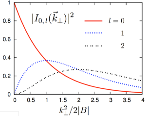
Figure 1: An example of the form factor function. We plot the $|I_{0,l}(\vec{k}_{\perp})|^{2}$ which will be used in the quark self-energy calculations. There the form factor is convoluted with the gluon propagator. The location of the maximum is $k_{\perp}^{2}=2l|B|$. For $l\geq 1$, the form factor suppresses the soft gluons, and this effect becomes stronger at larger $|B|$.

3 The renormalized quark self-energy at 1-loop

3.1 Renormalization

Now we use the Feynman rules in the Ritus bases to compute the higher orbital level contributions to the LLL quark self-energy. To deal with the UV divergence arising from summation of all higher orbital levels, we use the renormalized perturbation theory with counter terms which are determined in the $B=0$ case. Since the LLL kinetic term does not have $\gamma_{\perp}$, we will use the self-energy expression at $B=0$ for $p_{\perp}=0$ ($\Sigma^{R}$ and $\Sigma$ are the renormalized and bare self-energies, respectively),

$$\Sigma^{R}_{{\rm vac}}(p_{L};\mu)=\Sigma_{{\rm vac}}(p_{L})-\mathrm{i}\,\delta_{Z}(\mu)\,{\ooalign{\hfil/\hfil\crcr$p$}}_{L}+\delta m(\mu)\,.$$ (13)

where $\delta_{Z}(\mu)$ and $\delta m(\mu)$ are counter terms at scale $\mu$ to force the renormalized self-energy to vanish at $p_{L}^{2}=\mu^{2}$ (renormalization condition). It is implicit that $\Sigma_{{\rm vac}}$ depends on $\mu$ only through renormalized parameters, $m(\mu)$, $g(\mu)$, etc. For the self-energy at finite $B$, we must use the same counter terms as the $B=0$ case. Replacing the counter terms by $\Sigma^{R}_{{\rm vac}}(p_{L};\mu)-\Sigma_{{\rm vac}}(p_{L})$ through (13), we have the renormalized quark self-energy at finite $B$:

$$\Sigma_{B}^{R}(p_{L};\mu)=\Sigma_{{\rm vac}}^{R}(p_{L};\mu)+\left[\,\Sigma_{B}(p_{L})-\Sigma_{{\rm vac}}(p_{L})\,\right]\,.$$ (14)

The overall of the terms in the bracket is UV finite, and vanishes as $|B|\rightarrow 0$. The UV divergence is handled only through the first term.

Our computation requires an additional step, due to the need of separating the $l=0$ contribution. To do so, we first split the bare self-energies into two parts, depending on whether they contain contributions responsible for the $l=0$ level or not:

$$\Sigma_{B}=\delta\Sigma_{B}+\Sigma_{B}^{l=0}\,,~{}~{}~{}~{}\Sigma_{{\rm vac}}=\delta\Sigma_{{\rm vac}}+\Sigma_{{\rm vac}}^{l=0}\,,$$ (15)

with which we reorganize (14) as

$$\Sigma_{B}^{R}=\big{[}\,\Sigma_{{\rm vac}}^{R}-\Sigma_{{\rm vac}}^{l=0}\,\big{]}+\big{[}\,\delta\Sigma_{B}-\delta\Sigma_{{\rm vac}}\,\big{]}+\Sigma_{B}^{l=0}\,,$$ (16)

where the first two brackets contain contributions responsible for $l\geq 1$ levels, while the last term is responsible for the $l=0$ level. (How to identify $\Sigma^{l=0}_{{\rm vac}}$ will be shown later with an explicit example in Eq.(23)) Therefore it is natural to define

$$\Sigma_{B}^{R,\,l=0}\equiv\Sigma_{B}^{l=0}\,,$$ (17)

which is responsible for the $l=0$ contribution that is left for non-perturbative studies, and

$$\delta\Sigma_{B}^{R}\equiv\delta\Sigma_{{\rm vac}}^{R}+\left[\,\delta\Sigma_{B}-\delta\Sigma_{{\rm vac}}\,\right]\,,~{}~{}~{}~{}~{}\delta\Sigma_{{\rm vac}}^{R}\equiv\Sigma_{{\rm vac}}^{R}-\Sigma_{{\rm vac}}^{l=0}\,,$$ (18)

which include $l\geq 1$ contributions. Note that all terms in $\delta\Sigma_{B}^{R}$ are expressed in terms of $\delta\Sigma$, for which we can avoid the IR component of the gluon propagator. They will be the targets of our perturbative computations.

Here one might wonder why we also split the vacuum piece into $l=0$ and the others. Indeed, this is not a mandatory step. However, by adjusting the phase space for each of $B=0$ and $B\neq 0$ terms explicitly, trivial $B$-dependence coming from phase space mismatch can be avoided for each term, and we can extract out genuine $B$-dependent contributions for each phase space. This helps qualitative interpretations. Also, it becomes easier to see which renormalization scale should be taken to avoid the logarithmic enhancement typical in perturbation theory (see Eq.(27)).

3.2 An example of computation at finite $B$

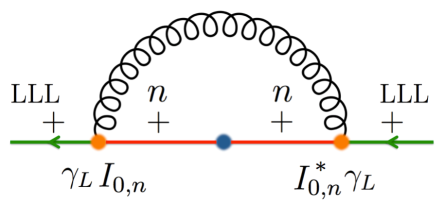
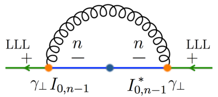
Figure 2: The one-loop corrections from the hLLs to the LLL. The Feynman gauge is chosen so that $D_{\mu\nu}\propto g_{\mu\nu}$. The summation over $n\geq 1$ is implicit. (Left) The spin conserving process. (Right) The spin flipping process. For the $n=1$ case, the soft gluon may appear and non-perturbative effects must be taken into account.

Before jumping to the results, it may be useful to show some example of computation based on the Ritus base. Below we use the gluon propagator in the Feynman gauge, $D_{\mu\nu}^{ab}(k)=g_{s}^{2}\delta^{ab}g_{\mu\nu}/\,k^{2}$, for simplicity. In this gauge we have only two types of diagrams shown in Fig.2. Below we demonstrate computations for the spin conserving process ($C_{F}=(N_{\rm c}^{2}-1)/2N_{\rm c}$):

$$\delta\Sigma_{B}^{{\rm sc}}(p_{L})=C_{F}g_{s}^{2}\,\sum_{n=1}\int_{k_{L}}\frac{\gamma_{L^{\prime}}\left[\,\mathrm{i}\left({\ooalign{\hfil/\hfil\crcr$p$}}_{L}-{\ooalign{\hfil/\hfil\crcr$k$}}_{L}\right)+m\,\right]\gamma_{L^{\prime}}}{\,(p_{L}-k_{L})^{2}+2n|B|+m^{2}\,}\int_{k_{\perp}}\frac{1}{\,n!\,}\left(\frac{k_{\perp}^{2}}{\,2|B|\,}\right)^{\!n}\mathrm{e}^{-\frac{k_{\perp}^{2}}{2|B|}}\,\frac{1}{\,k^{2}\,}\,,$$ (19)

where (12) is used and the complex phases of form factors cancel out. The sum starts from $l=n=1$ (For the spin flipping process, the sum starts from $l=n-1=1$). A few remarks are in order: (i) Since the quark propagator is independent of transverse momenta, the $k_{\perp}$ integral could be factorized; (ii) The form factor appears as powers of $(k_{\perp}/2|B|)^{n}$, so that the IR part of the gluon propagator is suppressed. A maximum of the form factor appears at $k_{\perp}^{2}=2n|B|$; (iii) The $\gamma_{2}$ matrix part of the quark propagator drops off due to the projection operator $\mathcal{P}_{+}$ attached to $\chi$-fields: $\mathcal{P}_{+}\gamma_{2}\mathcal{P}_{+}=0$. Furthermore, although specific to this process, only the term proportional to $m$ will survive after manipulating the $\gamma$-matrices.

As usual, we use the Feynman parameter $\zeta$ to integrate over $k_{L}$, and then get

$$\delta\Sigma_{B}^{{\rm sc}}(p_{L})=m\,\frac{\,C_{F}\alpha_{s}\,}{\,2\pi\,}\int_{0}^{1}\mathrm{d}\zeta~{}\delta K^{B}_{\zeta}\,,$$ (20)

where we have changed variables as $x=2|B|k_{\perp}^{2}$, and defined

$$\delta K^{B}_{\zeta}=\int_{0}^{\infty}\!\mathrm{d}x\,\sum_{n=1}\,\frac{\,x^{n}\,}{n!}\,\mathrm{e}^{-x}\,\frac{\,1\,}{\,\Delta_{\zeta}+(1-\zeta)x+\zeta n\,}\,,~{}~{}~{}~{}~{}\Delta_{\zeta}=\frac{\,\zeta(1-\zeta)p_{L}^{2}+\zeta m^{2}\,}{2|B|}\,.$$ (21)

The integral in $\delta K^{B}_{\zeta}$ contains two integration variables $(x,n)$. We reduce the integral from two to one dimension via proper time representation:

$$\delta K^{B}_{\zeta}=\, \int_{0}^{\infty}\!\mathrm{d}x\,\sum_{n=1}\,\frac{\,x^{n}\,}{n!}\,\mathrm{e}^{-x}\,\int_{0}^{\infty}\mathrm{d}\tau~{}\mathrm{e}^{-\tau\left[\Delta_{\zeta}+(1-\zeta)x+\zeta n\right]}\,$$

$$=\, \int_{0}^{\infty}\mathrm{d}\tau~{}\mathrm{e}^{-\tau\Delta_{\zeta}}\int_{0}^{\infty}\mathrm{d}x~{}\mathrm{e}^{-x\left[1+(1-\zeta)\tau\right]}\,\left(\sum_{n=0}\,\frac{\,\left(x\,\mathrm{e}^{-\tau\zeta}\right)^{n}\,}{n!}-1\right)\,$$

$$=\, \int_{0}^{\infty}\mathrm{d}\tau~{}\mathrm{e}^{-\tau\Delta_{\zeta}}\int_{0}^{\infty}\mathrm{d}x~{}\left(\mathrm{e}^{-x\left[1+(1-\zeta)\tau-\mathrm{e}^{-\tau\zeta}\right]}\,-\mathrm{e}^{-x\left[1+(1-\zeta)\tau\right]}\right)$$

$$=\, \int_{0}^{\infty}\mathrm{d}\tau~{}\left(\frac{\mathrm{e}^{-\tau\Delta_{\zeta}}}{\,1-\mathrm{e}^{-\tau\zeta}+(1-\zeta)\tau\,}-\frac{\mathrm{e}^{-\tau\Delta_{\zeta}}}{\,1+(1-\zeta)\tau\,}\right)\,.$$ (22)

The first term is singular at small $\tau$ which will be regulated by subtracting the vacuum piece.

3.3 Phase space separation at $B=0$

Having seen how the form factor function effectively restricts the integral over $k_{\perp}$, it is natural to identify $\Sigma_{{\rm vac}}^{{\rm sc},\,l=0}$ as (odd ${k}_{\perp}$ terms are dropped)

$$\Sigma_{{\rm vac}}^{{\rm sc},\,l=0}(p_{L})=C_{F}g_{s}^{2}\,\int_{k_{L}}\int_{k_{\perp}}\gamma_{L^{\prime}}\frac{\mathrm{i}\left({\ooalign{\hfil/\hfil\crcr$p$}}_{L}-{\ooalign{\hfil/\hfil\crcr$k$}}_{L}\right)+m}{\,(p_{L}-k_{L})^{2}+k_{\perp}^{2}+m^{2}\,}\gamma_{L^{\prime}}\times\mathrm{e}^{-\frac{k_{\perp}^{2}}{2|B|}}\,\frac{1}{\,k^{2}\,}\,,$$ (23)

which is responsible for the $l=0$ phase space, as seen from the fact that the $k_{\perp}^{2}$ integral is effectively cutoff by $\sim 2|B|$. We can get $\delta\Sigma_{{\rm vac}}^{{\rm sc}}$ by replacing $\mathrm{e}^{-k_{\perp}^{2}/2|B|}\rightarrow 1-\mathrm{e}^{-k_{\perp}^{2}/2|B|}$. The integral can be computed as before, and the resulting expression is

$$\left(\,\Sigma_{{\rm vac}}^{{\rm sc},\,l=0}\,,\delta\Sigma_{{\rm vac}}^{{\rm sc}}\,\right)=m\,\frac{\,C_{F}\alpha_{s}\,}{\,2\pi\,}\int_{0}^{1}\mathrm{d}\zeta\int_{0}^{\infty}\mathrm{d}\tau~{}\mathrm{e}^{-\tau\Delta_{\zeta}}\left(\frac{1}{\,1+\tau\,}\,,\,\frac{1}{\,\tau\,}-\frac{1}{\,1+\tau\,}\right)\,.$$ (24)

Here $\delta\Sigma_{{\rm vac}}^{{\rm sc}}$ is singular at small $\tau$ and becomes well-defined only after combining with the bare self-energy $\delta\Sigma_{B}^{{\rm sc}}$ at finite $B$. On the other hand, $\Sigma_{{\rm vac}}^{{\rm sc},\,l=0}$ blows up for small $p_{L}^{2}$, invalidating perturbation theory. It will be combined with the renormalized self-energy at $B=0$:

$$\Sigma_{{\rm vac}}^{R,\,{\rm sc}}(p_{L};\mu)=-m\,\frac{\,C_{F}\alpha_{s}\,}{\,2\pi\,}\int_{0}^{1}\mathrm{d}\zeta\,\ln\frac{\,(1-\zeta)\,p_{L}^{2}+m^{2}\,}{\,(1-\zeta)\,\mu^{2}+m^{2}\,}\,.$$ (25)

Similar to $\Sigma_{{\rm vac}}^{{\rm sc},\,l=0}$, this expression itself cannot be used for small $p_{L}^{2}$: The large logarithm must be avoided by taking $\mu^{2}\sim p_{L}^{2}$, but such small $\mu$ leads to large $\alpha_{s}(\mu)$, invalidating perturbation theory. In contrast, after subtracting $\Sigma_{{\rm vac}}^{{\rm sc},\,l=0}$ from this expression, it is possible to make the expression for $\delta\Sigma_{{\rm vac}}^{R}$ valid for all $p_{L}^{2}$. To see this, note that (for simplicity we ignore $m$ inside of the logarithm)

$$\Sigma_{{\rm vac}}^{{\rm sc},\,l=0}\sim\int_{0}^{\Delta_{\zeta}^{-1}}\!\mathrm{d}\tau~{}\frac{\,1\,}{\,1+\tau\,}=\ln\,\frac{\,\zeta(1-\zeta)p_{L}^{2}+2|B|\,}{\zeta(1-\zeta)p_{L}^{2}}\,,$$ (26)

this is combined with $\Sigma_{{\rm vac}}^{R,\,{\rm sc}}$ to yield

$$\delta\Sigma_{{\rm vac}}^{R,\,{\rm sc}}\sim-\int_{0}^{1}\mathrm{d}\zeta\,\ln\,\frac{\,\zeta(1-\zeta)p_{L}^{2}+2|B|\,}{\,\zeta(1-\zeta)\mu^{2}\,}~{}\rightarrow~{}-\ln\frac{\,2|B|\mathrm{e}^{2}\,}{\,\mu^{2}\,}\,~{}~{}~{}(p_{L}^{2}\rightarrow 0)\,.$$ (27)

In this expression, the large logarithm can be suppressed even for small $p_{L}^{2}$, by taking $\mu^{2}$ to be $\sim 2|B|\mathrm{e}^{2}\simeq 15|B|$ (more precise numerical computations give a smaller value, $\simeq 8.8|B|$, but it is still large). At the same time, if $2|B|\mathrm{e}^{2}\gg\Lambda_{\rm QCD}^{2}$, the perturbative expression for the renormalized parameters $\alpha_{s}(\mu),m(\mu),\cdots,$ remains valid. This result is rather natural because we have effectively introduced the IR cutoff by separating contributions from the $l=0$ levels. The appearance of the big factor ${\cal O}(10)$ has some resemblance to finite temperature calculations where the $\mu$ appropriate for perturbation theory has been supposed to be $\sim 2\pi T$ [18].

The above estimate for $\mu$ is based on the rather crude approximation, so we numerically search for the renormalization scale such that

$$\delta\Sigma_{{\rm vac}}^{R}(p_{L},\mu^{*})=0\,,~{}~{}~{}~{}~{}\mu^{*}=\mu^{*}\left(p_{L},|B|\right)\,,$$ (28)

where the logarithmic term disappears. Clearly $\mu^{*}$ is a function of $p_{L}$ and $B$, and we plot its behavior in Fig.3. Remarkably, even for the $p_{L}^{2}=0$ case, $\mu^{*}$ reaches $1\,{\rm GeV}$ already at $|B|\simeq 0.12\,{\rm GeV}^{2}$. Since we shall soon show that the other contribution, $\delta\Sigma_{B}-\delta\Sigma_{{\rm vac}}$, are at most of $\sim C_{F}\alpha_{s}/2\pi\times{\cal O}(1)$ irrespective to values of $p_{L}^{2}/|B|$, one can justify the perturbative expressions of $\delta\Sigma_{B}^{R}$ as far as $\alpha_{s}(\mu^{*})$ is small. Therefore we suppose that the contributions from higher orbitals do not strongly affect the LLL already at $|B|$ of $(0.1-0.3)\,{\rm GeV}^{2}$.

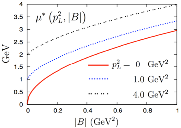
Figure 3: The optimized renormalization scale $\mu^{*}(p_{L}^{2},|B|)$ which satisfies $\delta\Sigma^{R}_{{\rm vac}}(p_{L};\mu^{*})=0$. At $|B|\simeq 0.12\,{\rm GeV}^{2}$, $\mu^{*}$ starts to go beyond $1.0\,{\rm GeV}$ for all $p_{L}^{2}$.

3.4 Results

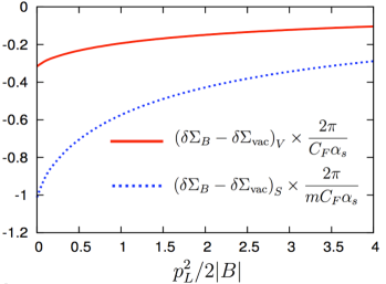
Figure 4: The $\delta\Sigma_{B}(p_{L})-\delta\Sigma_{{\rm vac}}(p_{L})$ for vector and scalar parts. To plot the $\mu$-independent part, we multiply factors $2\pi/C_{F}\alpha_{s}$ and $2\pi/mC_{F}\alpha_{s}$, respectively, and then set $m=0$. The main message is that these functions are regular and small in the entire range of $p_{L}^{2}/2|B|$.

Now we examine the self-energy at finite $B$ within the Feynman gauge. We write the vector and scalar self-energies separately, $\Sigma=-\mathrm{i}{\ooalign{\hfil/\hfil\crcr$p$}}_{L}\Sigma_{V}+\Sigma_{S}$. Adding contributions from the spin conserving and flipping processes, we arrive at expressions,

$$\left(\delta\Sigma_{B}^{R}\right)_{V} =\,\frac{\,C_{F}\alpha_{s}\,}{\,2\pi\,}\int_{0}^{1}\mathrm{d}\zeta~{}(1-\zeta)\,\bigg{\{}\left[\,-\ln\frac{\,(1-\zeta)\,p_{L}^{2}+m^{2}\,}{\,(1-\zeta)\,\mu^{2}+m^{2}\,}-\int_{0}^{\infty}\!\mathrm{d}\tau~{}\frac{\,\mathrm{e}^{-\tau\Delta_{\zeta}}\,}{\,1+\tau\,}\,\right]$$

$$~{}~{}~{}~{}~{}+\int_{0}^{\infty}\mathrm{d}\tau~{}\mathrm{e}^{-\tau\Delta_{\zeta}}\left[\,\frac{\mathrm{e}^{-\tau\zeta}}{\,1-\mathrm{e}^{-\tau\zeta}+(1-\zeta)\tau\,}-\frac{\mathrm{e}^{-\tau\zeta}}{\,1+(1-\zeta)\tau\,}-\frac{1}{\,\tau\,}+\frac{1}{\,1+\tau\,}\right]\bigg{\}}\,,$$ (30)

$$\left(\delta\Sigma_{B}^{R}\right)_{S} =m\,\frac{\,C_{F}\alpha_{s}\,}{\,2\pi\,}\int_{0}^{1}\mathrm{d}\zeta~{}\bigg{\{}\,2\left[\,-\ln\frac{\,(1-\zeta)\,p_{L}^{2}+m^{2}\,}{\,(1-\zeta)\,\mu^{2}+m^{2}\,}-\int_{0}^{\infty}\!\mathrm{d}\tau~{}\frac{\,\mathrm{e}^{-\tau\Delta_{\zeta}}\,}{\,1+\tau\,}\,\right]$$

$$~{}~{}~{}~{}~{}+\int_{0}^{\infty}\mathrm{d}\tau~{}\mathrm{e}^{-\tau\Delta_{\zeta}}\left[\,\frac{1+\mathrm{e}^{-\tau\zeta}}{\,1-\mathrm{e}^{-\tau\zeta}+(1-\zeta)\tau\,}-\frac{1+\mathrm{e}^{-\tau\zeta}}{\,1+(1-\zeta)\tau\,}-\frac{2}{\,\tau\,}+\frac{2}{\,1+\tau\,}\right]\bigg{\}}\,,$$ (31)

where the first bracket comes from $\delta\Sigma_{{\rm vac}}^{R}$, and the second from the difference between the bare self-energies, $\delta\Sigma_{B}-\delta\Sigma_{{\rm vac}}$.

We have already seen that $\delta\Sigma_{{\rm vac}}^{R}$ contains the logarithms largely related to the choice of the renormalization scale and can be eliminated at $\mu^{*}$. So let us look at the remaining contributions, i.e. the $(\delta\Sigma_{B}-\delta\Sigma_{{\rm vac}})$’s, which contain rather complicated integrals over $\tau$ and $\zeta$. We examine magnitudes and signs of the $(\delta\Sigma_{B}-\delta\Sigma_{{\rm vac}})$’s as shown in Fig.4. To plot the $\mu$-independent part, we multiply $2\pi/C_{F}\alpha_{s}$ ($2\pi/mC_{F}\alpha_{s}$) to the vector (scalar) part and then set $m(\mu)=0$. (Below we will always set $m=0$ inside the integrals. Introduction of the mass just makes perturbation theory work better.) Their values are small and regular in the entire domain of $p_{L}^{2}/2|B|$. Thus perturbative expressions for the $(\delta\Sigma_{B}-\delta\Sigma_{{\rm vac}})$’s are valid as far as $\alpha_{s}(\mu)$ is small, as already advertised.

These self-energies can be converted into the field strength and mass at finite $B$ through the following relations:

$$\frac{1}{\,1+\left(\delta\Sigma_{B}^{R}\right)_{V}\,}\equiv Z_{B}(p_{L};\mu)\,,~{}~{}~{}~{}~{}Z_{B}\left[\,1+\frac{\,\left(\delta\Sigma_{B}^{R}\right)_{S}\,}{m}\,\right]\,m(\mu)\equiv m_{B}(p_{L};\mu)\,.$$ (32)

We call $m_{B}$ “current quark mass” of the LLL. For the renormalized parameters at $B=0$, we use the 1-loop expressions for the running coupling and mass:

$$\alpha_{s}(\mu)=\frac{1}{\,4\pi\beta_{0}\ln(\mu^{2}/\Lambda_{\rm QCD}^{2})\,}\,,~{}~{}~{}m(\mu)=\left(\frac{\ln(\mu_{0}^{2}/\Lambda_{\rm QCD}^{2})}{\,\ln(\mu^{2}/\Lambda_{\rm QCD}^{2})\,}\right)^{\!\frac{\gamma_{m0}}{2\beta_{0}}}\,m(\mu_{0})\,,$$ (33)

where $\beta_{0}=(11N_{\rm c}-2N_{\rm f})/48\pi^{2}$ and $\gamma_{m0}=3C_{F}/(4\pi)^{2}$. In the following, we take $(N_{\rm c},N_{\rm f})=(3,\,5)$ and use the central value of $\Lambda_{\rm QCD}=\Lambda_{\overline{{\rm MS}}}^{N_{\rm f}=5}=(213\pm 8)\,{\rm MeV}$ [12].

In Fig.5, we show the behavior of $m_{B}$ for given $p_{L}^{2}$ and $B$. The $B=(0.02,\,0.1,\,0.3)\,{\rm GeV}^{2}$ cases are plotted. The function is divided by the current quark mass at $B=0$ renormalized at $\mu_{0}=2\,{\rm GeV}$. One can get the mass functions for each flavor by multiplying $m_{f}(2\,{\rm GeV})$ and rescaling $B_{f}(=e_{f}B)$ appropriately for each flavor.

As for the renormalization scale, we take $\mu$ to be $\sim\mu^{*}(p_{L}^{2},|B|)$ following the discussions around Eq.(27). We attach some errors by varying $\mu^{*}$ because the logarithmic terms of the higher order loops are not always eliminated by $\mu^{*}$ determined at 1-loop. We use the following procedure: First we suppose that $\mu^{*2}$ takes the form,

$$\mu^{*2}(p_{L}^{2},|B|)=p_{L}^{2}+C(p_{L}^{2})|B|+\cdots,$$ (34)

and compute $C(p_{L}^{2})$. Then we define $\mu_{\pm}^{*2}\equiv\mu^{*2}\pm 0.5\,C|B|$ and plot $m_{B}$ at $\mu_{\pm}^{*}$ to examine its renormalization scale dependence. The $\mu$-dependence is rather large for the $B=0.02\,{\rm GeV}^{2}$ case mainly due to the strong running of $\alpha_{s}$ at small $\mu^{*}$. On the other hand, for the $B=0.3\,{\rm GeV}^{2}$ case, $\mu^{*}$ is already large for $p_{L}^{2}=0$, $\mu^{*}\geq 1\,{\rm GeV}$, and there is no strong dependence on $\mu$.

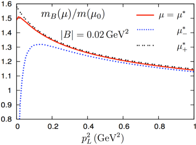
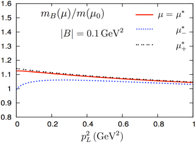
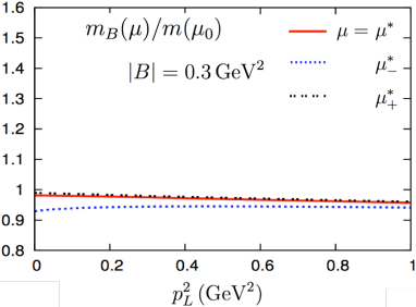
Figure 5: The “current quark mass” of the LLL, $m_{B}$, as a function of $p_{L}^{2}$. The function is normalized by the current quark mass at $B=0$, $m(\mu_{0})$ with $\mu_{0}=2\,{\rm GeV}$. We plot the $|B|=(0.02,\,0.1,\,0.3)\,{\rm GeV}^{2}$ cases. The renormalization scale is varied around $\mu^{*}$, see discussions around Eq.(34). As $|B|$ increases, the overall size as well as the $\mu$-dependence become smaller.

4 Conclusion

In this Letter we have developed a systematic scheme for preparing the renormalized parameters for the LLL fields from first-principle QCD, that will be inputs for forthcoming non-perturbative analyses. The form factors in the Ritus bases allow us to apply perturbation theory in evaluating the coupling between the LLL and higher orbital levels. The renormalization for the quark self-energy is done by summing up all higher orbital levels in a model independent manner.

The results indicate that the higher orbital levels cease to strongly affect the LLL at rather small value of $|eB|$, $(0.1-0.3)\,{\rm GeV}^{2}$. It is tempting to compare this estimate with lattice data for the chiral condensate where characteristic changes are observed around $|eB|\sim 0.3\,{\rm GeV}^{2}$. We conjecture that the changes can be attributed to the separation of the hLLs from the LLL.

To extract real phenomenological interpretations from our perturbative results, however, we still need further studies of other renormalized parameters, effective operators, and the OPE for soft gluons. The extension to higher loops is also a very important issue to check whether systematics is at work. Indeed, beyond 1-loop, there are subdiagrams with soft gluons even after separating the $l=0$ levels. We leave them for future studies.

References

- [1] For review, I. A. Shovkovy, arXiv:1207.5081 [hep-ph].
- [2] H. Suganuma and T. Tatsumi, Annals Phys. 208 (1991) 470; V. P. Gusynin, V. A. Miransky and I. A. Shovkovy, Phys. Lett. B 349 (1995) 477 [hep-ph/9412257]; ibid. Nucl. Phys. B 462 (1996) 249 [hep-ph/9509320].
- [3] F. Bruckmann, G. Endrodi and T. G. Kovacs, JHEP 1304 (2013) 112 [arXiv:1303.3972 [hep-lat]]; G. S. Bali, F. Bruckmann, G. Endrodi, F. Gruber and A. Schaefer, JHEP 1304 (2013) 130 [arXiv:1303.1328 [hep-lat]].
- [4] Y. Hidaka and A. Yamamoto, Phys. Rev. D 87, 094502 (2013) [arXiv:1209.0007 [hep-ph]]; M. A. Andreichikov, B. O. Kerbikov, V. D. Orlovsky and Y. A. Simonov, arXiv:1304.2533 [hep-ph]; M. A. Andreichikov, V. D. Orlovsky and Y. A. Simonov, arXiv:1211.6568 [hep-ph].
- [5] P. V. Buividovich, M. N. Chernodub, D. E. Kharzeev, T. Kalaydzhyan, E. V. Luschevskaya and M. I. Polikarpov, Phys. Rev. Lett. 105 (2010) 132001 [arXiv:1003.2180 [hep-lat]]; K. Fukushima and Y. Hidaka, Phys. Rev. Lett. 110 (2013) 031601 [arXiv:1209.1319 [hep-ph]]; M. N. Chernodub, Phys. Rev. D 82 (2010) 085011 [arXiv:1008.1055 [hep-ph]].
- [6] K. Fukushima and J. M. Pawlowski, Phys. Rev. D 86 (2012) 076013 [arXiv:1203.4330 [hep-ph]].
- [7] P. V. Buividovich, M. N. Chernodub, E. V. Luschevskaya and M. I. Polikarpov, Phys. Lett. B 682 (2010) 484 [arXiv:0812.1740 [hep-lat]].
- [8] G. S. Bali, F. Bruckmann, G. Endrodi, Z. Fodor, S. D. Katz, S. Krieg, A. Schafer and K. K. Szabo, JHEP 1202 (2012) 044 [arXiv:1111.4956 [hep-lat]].
- [9] T. Kojo and N. Su, Phys. Lett. B 720 (2013) 192 [arXiv:1211.7318 [hep-ph]].
- [10] G. S. Bali, F. Bruckmann, G. Endrodi, Z. Fodor, S. D. Katz and A. Schafer, Phys. Rev. D 86 (2012) 071502 [arXiv:1206.4205 [hep-lat]]; V. V. Braguta, P. V. Buividovich, T. Kalaydzhyan, S. V. Kuznetsov and M. I. Polikarpov, Phys. Atom. Nucl. 75 (2012) 488 [arXiv:1011.3795 [hep-lat]]; M. D’Elia and F. Negro, Phys. Rev. D 83 (2011) 114028 [arXiv:1103.2080 [hep-lat]].
- [11] B. L. Ioffe and A. V. Smilga, Nucl. Phys. B 232 (1984) 109; N. O. Agasian and I. A. Shushpanov, Phys. Lett. B 472 (2000) 143 [hep-ph/9911254]; T. D. Cohen, D. A. McGady and E. S. Werbos, Phys. Rev. C 76 (2007) 055201 [arXiv:0706.3208 [hep-ph]]; J. O. Andersen, JHEP 1210 (2012) 005 [arXiv:1205.6978 [hep-ph]].
- [12] J. Beringer et al. [Particle Data Group], Phys. Rev. D 86 (2012) 010001.
- [13] M. A. Shifman, A. I. Vainshtein and V. I. Zakharov, Nucl. Phys. B 147 (1979) 385; V. A. Novikov, M. A. Shifman, A. I. Vainshtein, M. B. Voloshin and V. I. Zakharov, Nucl. Phys. B 237 (1984) 525; V. A. Novikov, M. A. Shifman, A. I. Vainshtein and V. I. Zakharov, Fortsch. Phys. 32 (1984) 585.
- [14] V. P. Gusynin and A. V. Smilga, Phys. Lett. B 450 (1999) 267 [hep-ph/9807486].
- [15] E. J. Ferrer and V. de la Incera, Phys. Rev. Lett. 102 (2009) 050402 [arXiv:0807.4744 [hep-ph]]; Nucl. Phys. B 824 (2010) 217 [arXiv:0905.1733 [hep-ph]].
- [16] D. K. Hong, Y. Kim and S. -J. Sin, Phys. Rev. D 54 (1996) 7879 [hep-th/9603157]; G. W. Semenoff, I. A. Shovkovy and L. C. R. Wijewardhana, Phys. Rev. D 60 (1999) 105024 [hep-th/9905116]; V. Skokov, Phys. Rev. D 85 (2012) 034026 [arXiv:1112.5137 [hep-ph]].
- [17] X. -G. Wu, S. J. Brodsky and M. Mojaza, arXiv:1302.0599 [hep-ph].
- [18] J. -P. Blaizot, E. Iancu and A. Rebhan, In *Hwa, R.C. (ed.) et al.: Quark gluon plasma* 60-122 [hep-ph/0303185]; U. Kraemmer and A. Rebhan, Rept. Prog. Phys. 67 (2004) 351 [hep-ph/0310337]; J. O. Andersen and M. Strickland, Annals Phys. 317 (2005) 281 [hep-ph/0404164]; N. Su, Commun. Theor. Phys. 57 (2012) 409 [arXiv:1204.0260 [hep-ph]].
- [19] K. Hattori and K. Itakura, Annals Phys. 330 (2013) 23 [arXiv:1209.2663 [hep-ph]]; ibid 334 (2013) 58 [arXiv:1212.1897 [hep-ph]].
- [20] K. -I. Ishikawa, D. Kimura, K. Shigaki and A. Tsuji, arXiv:1304.3655 [hep-ph].